Interplay of diffraction and nonlinear effects in propagation of ultrashort pulses

Abstract

We investigate the interplay of diffraction and nonlinear effects during propagation of very short light pulses. Adapting the factorization approach to the problem at hand by keeping the transverse-derivative terms apart from the residual nonlinear contributions we derive an unidirectional propagation equation valid for weak dispersion and reducing to the slowly-evolving-wave-approximation for the case of paraxial rays. Comparison of numerical simulation results for the two equations shows pronounced differences when self-focusing plays important role. We devote special attention to modelling propagation of ultrashort terahertz pulses taking into account diffraction as well as Kerr type and second order nonlinearities. Comparing measured and simulated wave forms we deduce the value of the nonlinear refractive index of lithium niobate in the terahertz region to be three orders of magnitude larger than in the visible.

Keywords: nonlinear propagation, diffraction, Kerr effect

1 Introduction

Improving theoretical description of propagation of light pulses consisting of just a few cycles has received considerable interest in the past two decades [1, 2, 3, 4, 5, 6, 7, 8, 9, 10, 11]. However, relatively small number of investigations consider the variation in the transverse directions i.e. the diffraction effects. For example, analytical solutions are presented in [3] for diffraction and dispersion effects but only for the case of linear propagation. Our aim is to consider both nonlinear effects and transverse variation leading to broadening in the transverse direction but also self focusing for high intensities for the case when dispersion effects including attenuation have a minor role.

Introducing additional dependence on one or both transverse coordinates makes mathematical modelling and numerical simulations more involved but is necessary for studying effects like self-guiding and filament formation when competition between diffraction and nonlinearity plays important role [12, 13, 14, 15, 16]. Nonlinear envelope equations of the type derived in [1] were used for numerical simulation of shape effects [12] on the propagation of femtosecond pulses in media with weak dispersion and for studying filament stability [14]. Analytical approach using soliton solutions can also be used for filament propagation description [16] and collision-dynamics study of otical pulses [15] for certain fixed values of the nonlinear coefficient. Taking into account both the transverse (as well as longitudinal) profile and nonlinearity is essential in describing interaction of optical and matter-wave soliton solutions characterizing trapped-atom arrangements [13].

Examination of the term containing the transverse derivatives reveals that in the traditional slowly-varying-envelope approximation an implicit expansion in the transverse components of the wave vector is made by assuming that they are much smaller than the longitudinal component pointing in the propagation direction [17]. This approximate treatment of transverse dependence also characterizes for example the slowly-evolving-wave approximation (SEWA) introduced in [1] as pointed out in [6]. We avoid this expansion pertaining to paraxial-ray approximation by modifying the factorization approach of Kinsler [10] to obtain an evolution equation suitable for numerical calculation which properly takes into account diffraction including space-time focusing effects.

2 Theoretical considerations

To obtain an unidirectional propagation equation we follow the approach outlined in [10] and discussed earlier in more detail in [18]. We represent the physical electric field ${\bi E}_{ph}({\bi r},t)$ by analytic complex field ${\bi E}({\bi r},t)$ whose Fourier transform contains only positive frequencies [19, 20]:

$${\bi E}_{ph}({\bi r},t)=\frac{1}{2}\left[{\bi E}({\bi r},t)+\mbox{c.c.}\right].$$ (1)

Taking the propagation direction to be the $z$ axis the 3-dimensional wave eqation can be written as

$$\left(\partial_{z}^{2}+\nabla_{\perp}^{2}\right){\bi E}({\bi r},t) - \frac{1}{c^{2}}\frac{\partial^{2}}{\partial t^{2}}\epsilon_{L}(t)\star{\bi E}({\bi r},t)=\frac{4\pi}{c^{2}}\frac{\partial^{2}}{\partial t^{2}}{\bi P}_{NL}({\bi E},{\bi r},t)$$ (2)

$$+ \mu_{0}\frac{\partial{\bi J}({\bi r},t)}{\partial t}+\bi\nabla\,\bi\nabla\cdot{\bi E}({\bi r},t)$$

where $\star$ denotes convolution, $\epsilon_{L}$ contains the linear part of the material response, ${\bi P}_{NL}({\bi E},{\bi r},t)$ is the nonlinear polarization, ${\bi J}({\bi r},t)$ the current density and we assumed a non-magnetic material. Transforming into wave-vector and frequency space we can write (2) as

$$\left(-k_{z}^{2}-k_{\perp}^{2}+\beta^{2}\right){\bi E}({\bi k},\omega)=-{\bi Q},$$ (3)

with $-{\bi Q}$ denoting all terms corresponding to the right-side of (2) and $\beta^{2}=\omega^{2}\epsilon_{L}(\omega)/c^{2}$. Note that in contrast to [10] we do not place the term with transverse derivatives in the residual term ${\bi Q}$ but keep it exlicitly. Performing the factorization in (3):

$$\left(k_{z}-\sqrt{\beta^{2}-k_{\perp}^{2}}\right)\left(k_{z}+\sqrt{\beta^{2}-k_{\perp}^{2}}\right){\bi E}({\bi k},\omega)={\bi Q},$$ (4)

we can express ${\bi E}$ as a sum of two terms:

$${\bi E}({\bi k},\omega)=\frac{1}{2\sqrt{\beta^{2}-k_{\perp}^{2}}}\left(\frac{1}{k_{z}-\sqrt{\beta^{2}-k_{\perp}^{2}}}-\frac{1}{k_{z}+\sqrt{\beta^{2}-k_{\perp}^{2}}}\right){\bi Q}.$$ (5)

Defining ${\bi E}^{(\pm)}$ by

$${\bi E}^{(\pm)}({\bi k},\omega)=\frac{\pm 1}{2\sqrt{\beta^{2}-k_{\perp}^{2}}}\,\frac{1}{k_{z}\mp\sqrt{\beta^{2}-k_{\perp}^{2}}}{\bi Q}$$ (6)

we can write ${\bi E}={\bi E}^{(+)}+{\bi E}^{(-)}$ where ${\bi E}^{(\pm)}$ obey the equations:

$$\left(k_{z}\mp\sqrt{\beta^{2}-k_{\perp}^{2}}\right){\bi E}^{(\pm)}({\bi k},\omega)=\frac{\pm 1}{2\sqrt{\beta^{2}-k_{\perp}^{2}}}{\bi Q}.$$ (7)

Transforming back to ordinary space with respect to $k_{z}$ (but not ${\bi k}_{\perp}$) we obtain the two equations governing propagation of ${\bi E}^{(\pm)}(z,{\bi k}_{\perp},\omega)$:

$$\partial_{z}{\bi E}^{(\pm)}(z,{\bi k}_{\perp},\omega)=\pm\rmi\sqrt{\beta^{2}-k_{\perp}^{2}}{\bi E}^{(\pm)}(z,{\bi k}_{\perp},\omega)\pm\frac{\rmi}{2\sqrt{\beta^{2}-k_{\perp}^{2}}}\,{\bi Q}.$$ (8)

Equations (8) can be regarded as an alternative derivation of the unidirectional pulse propagation equation of Kolesik and Moloney [7] which is based on modal expansion of the fields. A potential disadvantage of relying on result (8) is that one has to work in the perpendicular wave vector space and without expansion one can not meaningfully transform to perpendicular derivatives in the ordinary space. Since our final intention is to arrive at an unidirectional propagation equation using only the forward propagating field ${\bi E}^{(+)}$ we have to mention an important constraint arising from attenuation taken into account through the (positive) imaginary part of $\beta^{2}(\omega)$. That term provides suppression for the forward propagating component but as seen form (8) it enhances the backward propagating term. Poor phase matching is expected to provide suppression for backward propagation but for long enough propagation distances compared to attenuation length that component may be amplified enough in order to make its effect through nonlinearity non-negligible. As a consequence, for the applicability of the unidirectional equation we require the condition of weak dispersion to be satisfied for the full frequency spectrum of the pulse and the propagation distance to be shorter than the attenuation length. This is in accordance with constraints on the applicability of the slowly-evolving-wave-approximation [1] concerning weak dispersion and restricted propagation length as discussed in [21] and section 11.6 of [22].

For a general transverse dependence one can use the cartesian components of the transverse wave vector $k_{x},k_{y}$ and the corresponding eigenfunctions $\exp(ik_{x}x+ik_{y}y)$ as in [7]. However, since our main interest resides in cylindrically symmetric pulse profiles we exploit that symmetry to make the numerical modelling less computationally intensive and use the simulation with arbitrary transverse dependence only as a check of numerical procedures.

We make the transformation to transverse wave vector space using the fact that the solution of the eigenvalue problem

$$\nabla_{\perp}^{2}f(r,\phi)+k_{\perp}^{2}f(r,\phi)=0,$$ (9)

with $r,\phi,z$ being the cylindrical coordinates, is [23]:

$$f(r,\phi)=\sum_{m=0}^{\infty}\left[A_{m}\,J_{m}(k_{\perp}r)+B_{m}\,N_{m}(k_{\perp}r)\right]e^{im\phi},$$ (10)

where $J_{m}$ is the Bessel function and $N_{m}$ is the Neumann function of order $m$. Assuming uniform medium in the transverse direction and regularity of the solution at $r=0$ with rotational symmetry around the $z$ axis means that only the $J_{0}$ term survives. We can thus expand the transverse dependence as

$$f(r)=\int_{0}^{\infty}A(k_{\perp})\,J_{0}(k_{\perp}r)\rmd k_{\perp}$$ (11)

and using the integral relation

$$\int_{0}^{\infty}rJ_{0}(k^{\prime}_{\perp}r)\,J_{0}(k_{\perp}r)\rmd r=\frac{1}{k_{\perp}}\delta(k^{\prime}_{\perp}-k_{\perp}),$$ (12)

where $\delta(k)$ is the Dirac delta function, we can invert (11) to get

$$A(k_{\perp})=k_{\perp}\int_{0}^{\infty}rf(r)J_{0}(k_{\perp}r)\rmd r.$$ (13)

There is an alternative approach to expression (11) which relies on explicit compactification of the transverse coordinate. Even without a strict boundary condition that the electric field vanishes at a fixed $r$ value, we may require that it be zero at some (large) value of $r=a$. That condition restricts the continuous integration variable in (11) to discreet values $k_{m}^{\perp}$ satisfying the condition $J_{0}(k_{m}^{\perp}a)=0$ and thus leads to

$$f(r)=\sum_{m=1}^{\infty}A_{m}\,J_{0}(k_{m}^{\perp}r).$$ (14)

Denoting the zeros of the Bessel function $J_{0}(x)$ by $x_{m},\;m=1,2,3,\ldots$ we can write $k_{m}^{\perp}=x_{m}/a$. Using the orthogonality relation [24]

$$\int_{0}^{a}rJ_{0}(x_{m}r/a)\,J_{0}(x_{n}r/a)\rmd r=\frac{a^{2}}{2}J_{1}(x_{n})^{2}\,\delta_{nm}$$ (15)

one can compute the expansion coefficients:

$$A_{m}=\frac{2}{a^{2}J_{1}(x_{m})^{2}}\,\int_{0}^{a}rf(r)J_{0}(x_{m}r/a)\rmd r.$$ (16)

We used this approach as a check of numerical implementation based on (11) and indeed ascertained that in our numerical simulations the above two approaches give indistinguishable results if the value $a$ of the radius at which the field vanishes is chosen large enough and for considered limited propagation distances. We acknowledge that the above compactification should be regarded only as an approximate numerical procedure and used with care since it leads to violation of general integral properties [25, 26, 27] of angular-spectrum representation for diffracted wave fields.

If the residual term on the right side of (7) does not mix the forward propagating field ${\bi E}^{(+)}$ with the backward propagating ${\bi E}^{(-)}$ considerably, i.e. it is small compared to propagation terms not mixing the two field components then one can decouple the corresponding equations for forward and backward propagation.

When taking into account both forward and backward propagating fields introduction of envelopes with slower spatial (in the $z$ direction) variation does not bring any real advantage since that introduces fast varying contributions in the residual term which mixes the two fields.

If the mixing of forward and backward propagating fields through the residual term is small enough so that a unidirectional propagation applies to good accuracy it is advantageous to introduce the envelope ${\bi A}(z,{\bi r}_{\perp},t)$ with slower $z$ and $t$ variation than the (complex) field itself through

$${\bi E}^{(+)}(z,{\bi r}_{\perp},t)={\bi A}(z,{\bi r}_{\perp},t)\,\exp[\rmi(\beta_{0}z-\omega_{0}t)],$$ (17)

where $\omega_{0}$ is the predetermined central (carrier) frequency and $\beta_{0}=n(\omega_{0})\omega_{0}/c$. In this way (8) for the forward propagating field is replaced by the following expression:

$$\partial_{z}{\bi A}(z,{\bi k}_{\perp},\omega) = \rmi(\sqrt{\beta^{2}-k_{\perp}^{2}}-\beta_{0}){\bi A}(z,{\bi k}_{\perp},\omega)$$ (18)

$$+ \frac{\rmi}{2\sqrt{\beta^{2}-k_{\perp}^{2}}}\,{\bi Q}_{A}({\bi A}),$$

with the residual term on the right side depending also on the envelope. It is customary to introduce the moving frame by transforming to new time $\tau$ and longitudinal distance $\zeta$ variables [1]:

$$\tau=t-\beta_{1}z,\;\zeta=z,$$ (19)

with $v_{g}(\omega_{0})=1/\beta_{1}$ the group velocity at $\omega_{0}$. The unidirectional envelope evolution equation (18) then becomes

$$\partial_{\zeta}{\bi A}(\zeta,{\bi k}_{\perp},\omega) = \rmi\left[\sqrt{\beta^{2}-k_{\perp}^{2}}-\beta_{0}-\beta_{1}\omega\right]{\bi A}(\zeta,{\bi k}_{\perp},\omega)$$ (20)

$$+ \frac{\rmi}{2\sqrt{\beta^{2}-k_{\perp}^{2}}}\,{\bi Q}_{A}({\bi A}).$$

3 Numerical simulation

We now turn to numerical simulation of light pulse propagation. As a first example we consider the case examined in [1] but without diffraction effects being taken into account there. A Kerr type nonlinearity is assumed with electric field and nonlinear polarization having the same direction. This is a reasonable approximation since the nonlinear effect in itself is small and including a small correction in the form of projection on the electric field vector is not expected to be significant [7]. In our simulations we do distinguish the transverse and longitudinal components of the electric field with respect to the axis of propagation based on values of the length of wave vector and its transverse component and add up these two components of electric field separately. However, for the cases studied numerically in the following we observe that this separation of transverse and longitudinal components gives noticeable difference compared to the case when neglecting it only for large enough transverse-coordinate values where typically the electric field magnitude drops to 1–2% of its central value. After transforming to $\omega$ (i.e. $\beta(\omega)$) and $k_{\perp}$ space the scalar form of (20) is thus appropriate:

$$\partial_{\zeta}A(\zeta,{\bi k}_{\perp},\omega) = \rmi\left[\sqrt{\beta^{2}-k_{\perp}^{2}}-\beta_{0}-\beta_{1}\omega\right]A(\zeta,{\bi k}_{\perp},\omega)$$ (21)

$$+ \frac{2\pi\rmi(\omega+\omega_{0})^{2}}{c^{2}\sqrt{\beta^{2}-k_{\perp}^{2}}}\,B(A),$$

where the nonlinear polarization has been written as

$$P_{NL}(z,{\bi r}_{\perp},t)=A_{NL}(z,{\bi r}_{\perp},t,A)\,\exp[\rmi(\beta_{0}z-\omega_{0}t)]+\mbox{c.c.},$$

and $B(A)$ is the Fourier transform of $A_{NL}$ to frequency and perpendicular wave vector space. If we expand $\sqrt{\beta^{2}-k_{\perp}^{2}}$ in the first term of (21) to linear order in $k^{2}_{\perp}$ and in the term containing $k^{2}_{\perp}$ approximate the refractive index $n(\omega)$ with its value at the carrier frequency $\omega_{0}$ we recover the linear terms of the SEWA equation (6) in [1]. We also recover the nonlinear term in that equation if in our nonlinear term we put $k_{\perp}$ to zero and again take the refractive index frequency independent and equal to its value at $\omega_{0}$. Simulation results show that these simplifications are quite good approximations for the case considered in [1] consisting of a pulse with central wavelength $\lambda_{0}=0.8\;\mu$m propagating in fused silica with a hyperbolic-secant shaped envelope $A_{s}(t)=1/\cosh\,[1.76t/\tau_{p}]$ and $\tau_{p}=2.67\;$fs. However, pronounced difference characterizes the solutions of the two equations when nonlinearity induced self focusing plays important role. In order to allow for dispersion and diffraction effects to develop over larger propagation distance we decreased the peak intensity used in [1] by a factor of two to $2\times 10^{13}\;\mbox{W/cm}^{2}$ for analyzing propagation in a Kerr medium with $A_{NL}=(2\pi)^{-1}n_{0}n_{2}|A|^{2}A$ where $n_{2}=3\times 10^{-13}\;$cm²/W is the nonlinear index of refraction and $|A|^{2}$ is normalized to give the intensity.

We observe that considering the propagation to be lossless for the above pulse properties and propagation distances not exceeding 100$\;\mu$m is a very good approximation since the imaginary part of the refractive index of considered silica glass in the frequency interval where the spectral distribution of the pulse is not less than 2% of its maximum is not exceeding 0.0004 [28] implying an attenuation length larger than 1500$\;\mu$m and even at the cut-off wavelength $\lambda_{m}=5.3\;\mu$m (see caption of figure 1) it is 140$\;\mu$m. In case of strong dispersion or propagation distances exceeding the attenuation length more careful treatment is required prefering solution of the full nonlinear wave equation [29].

We start by analyzing propagation of a beam with Gaussian transverse distribution whose amplitude is proportional to $\exp[-r^{2}/(2a_{r}^{2})]$ with $a_{r}=3\;\mu$m. The transverse-derivative term in expression (6) of [1] contains the term $\omega+\omega_{0}$ in the denominator and thus diverges when the envelope spectrum extends close to $-\omega_{0}$ which can be the case for single-cycle pulses. It is also present in the studied example which means that in order to avoid overflow during iterations one has to implement a cut-off for $\omega+\omega_{0}$ values approaching zero. Our simulations show that this value can be significantly smaller than $\omega_{0}$ (for example $0.1\omega_{0}$) without causing numerical problems. In order to avoid underestimation of the electric field the cut-off should be significantly smaller than the value at which the envelope falls to one half of its maximum as illustrated by figure 1. In that figure we compare results for different cut-off values after propagation distances of $40\;\mu$m and $80\;\mu$m at central ($r=0$) position. We observe similar relative differences for off-axis positions. For a stronger focused beam with $a_{r}=1\;\mu$m the differences are even larger.

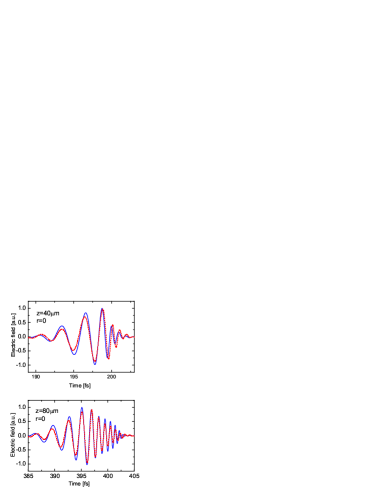
Figure 1: Electric field at $z=40\;\mu$m (upper panel) and $z=80\;\mu$m (lower panel) for $r=0$. The full line corresponds to the cut-off wavelength $\lambda_{m}=5.3\;\mu$m while the dash line is for $\lambda_{m}=1.04\;\mu$m which corresponds to the (lower) frequency at which the envelope takes one half of its maximum value.

In the following comparisons we use the cut-off value $\lambda_{m}=5.3\;\mu$m which leaves out only 0.5% of the envelope spectral distribution. We remark that in our result (20) the propagation condition $\beta>k_{\perp}$ applies and in the diverging nonlinear term there is no need to impose constraint on the lower limit of $|\beta-k_{\perp}|$ due to the integrable nature of the singularity.

Next, we compare the transverse profiles of the pulse by plotting the fluence as function of transverse coordinate after different propagation distances using the solution of (21) and of the corresponding expression (6) of [1]. We calculate the fluence by integrating $|E(z,r,\omega)|^{2}$ over the frequency $\omega$. Figure 2 shows the transverse fluence profiles for different propagation distances starting with a Gaussian amplitude distribution $\exp[-r^{2}/(2a_{r}^{2})]$ with $a_{r}=3.5\;\mu$m.

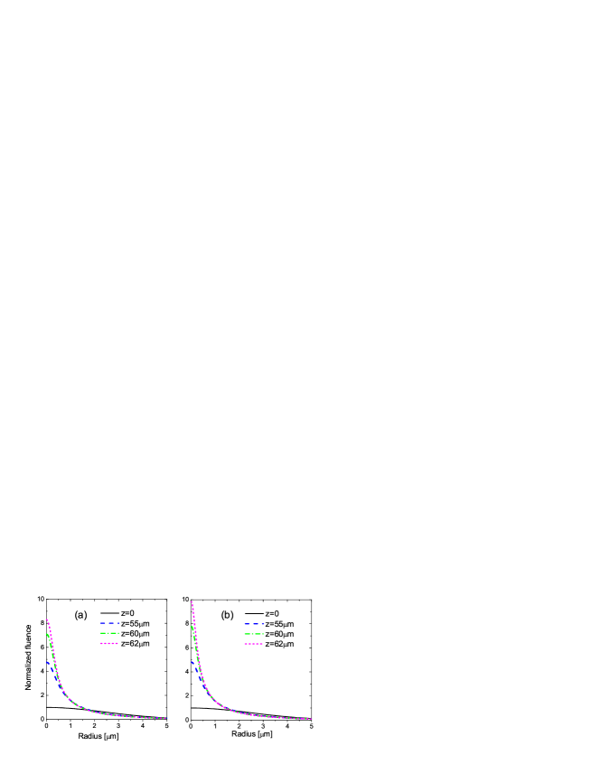
Figure 2: Transverse fluence profiles for initial distribution with $a_{r}=3.5\;\mu$m. Our result (a) and using the result from integrating the corresponding equation (6) of [1] (b).

In figure 2 we see the effect of self focusing which is dominant if the intensity is sufficiently high and the focusing of incoming pulse not too strong. The influence of the initial shape of the pulse on the propagation is quite important similarly to the case when femtosecond pulses propagate in air [12, 14]. We remark that in case of studied pronounced self focusing the resultant fluence can be quite high and not far from but not reaching the damage limit for fused silica [30]. In figure 3 we compare the time dependence of the electric field of the pulse after propagating $62\;\mu$m at $r=0$ using the two approaches.

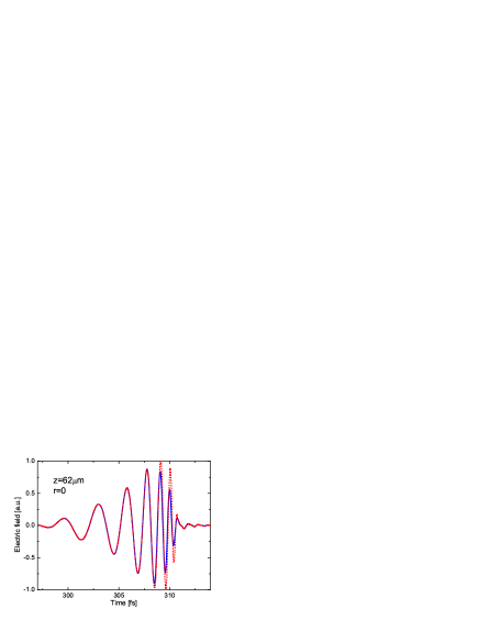
Figure 3: Time dependence of the electric field at $r=0$ after propagation of $62\;\mu$m. Solid line is our result and dash line is obtained by using the result of the equation from [1].

Our results are in general close to the results obtained by using the SEWA approach. However, in case of pronounced self focusing corresponding to propagating $z\approx 60\;\mu$m we observe that SEWA leads up to 20% larger central fluence values compared to our result. It is not difficult to understand the cause of this behaviour by recalling that SEWA amounts to dropping the transverse component of the wave vector in the square root of the nonlinear term in equation (20) thus diminishing the magnitude of that contribution for field components with nonzero transverse coordinate. This in turn leads to relative enhancement of the nonlinear effect for the central region of pulse. We can see from figure 3 that this enhancement comes from larger electric-field amplitude in the descending part of the envelope while the self-phase-modulation effect does not show noticeable difference. We also observe pronounced difference between the two approaches for large enough values of the transverse coordinate where the electric field is typically two orders of magnitude smaller than at central position. In this off-axis region SEWA typically underestimates the electric-field magnitude.

We now turn to analyzing terahertz single-cycle pulse propagation as exemplified by observation of nonlinear lattice response in [31] where a pulse with peak intensity of 100 MW/cm² was transmitted through a 2 mm thick LiNbO₃ crystal cooled to 80K. Based on the measured incoming (reference) electric field strength we construct a complex envelope function by retaining only the positive-frequency part of the Fourier transform and then introducing a shift by the carrier frequency $\omega_{0}=3.75\;$ps^-1 obtained using the formula $\omega_{0}=\int_{0}^{\infty}\omega|E(\omega)|^{2}\rmd\omega/\int_{0}^{\infty}|E(\omega)|^{2}\rmd\omega$. The measured reference electric field and the one calculated using the envelope function, together with its shape are shown in figure 4.

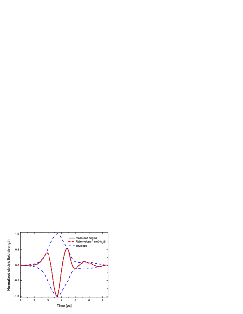
Figure 4: The envelope function (dash line) and the measured electric field (solid line) together with the electric field calculated using the envelope function.

In figure 5 the observed transmitted field strength is shown next to the reference one and the simulated result assuming linear propagation with and without absorption and with frequency-dependent refractive index of the form $n=A+b\,f^{2}+C\,f^{4}$ with $A=4.73,\;B=1.5\,10^{-5},\;C=8.5\,10^{-10}$ and $f\equiv\omega/(2\pi c)$ with $\omega/c$ expressed in cm^-1 [32].

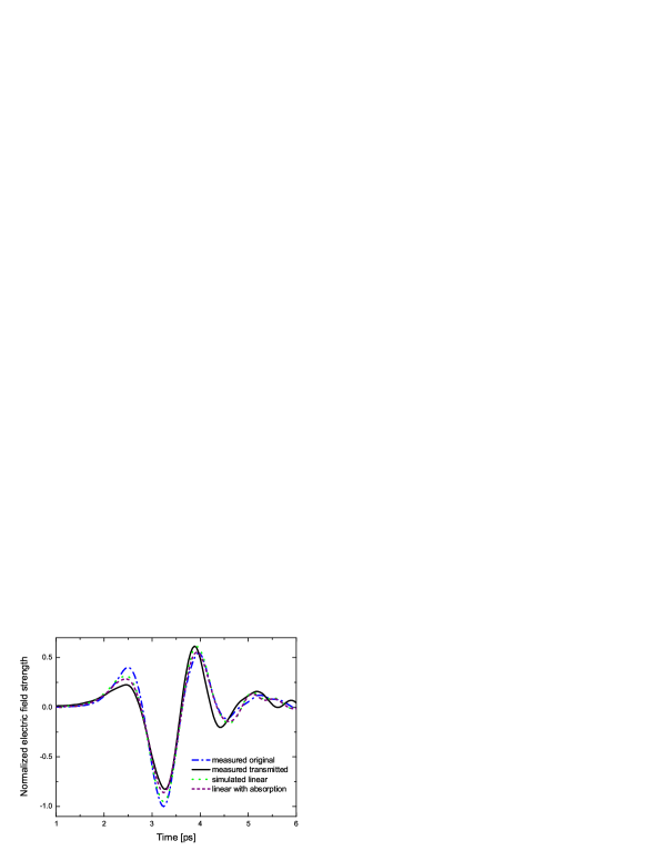
Figure 5: The measured original (dash-dot line), the measured transmitted electric field (solid line) and the calculated transmitted field assuming linear propagation with dispersion from [32] without absorption (dot line) and with absorption coefficient $\alpha=1\;$cm^-1 (dash line).

In this example absorption is not completely negligible but has a small effect as seen from figure 5 and measurements reported in [32]. Comparing the incoming and the transmitted pulse we conclude that the absorption coefficient at the carrier frequency should be $\alpha(\omega_{0})\approx 1\;$cm^-1 and taking into account the measured increase with frequency [32] we arrive at the value $\alpha(\omega_{m})\leq 1.5\;$cm^-1 where $\omega_{m}\approx 8\;$ps^-1 is the frequency at the effective upper limit of the frequency spectrum of the pulse. Since the real part of the propagation constant $\beta_{r}(\omega_{m})\approx 1200\;$cm^-1 we ascertain that the condition of weak dispersion is satisfied at the high end of spectrum and also for smaller frequencies characterizing the pulse (measurements extending down to 0.25 THz did not show increase of absorption coefficient [33]). We also observe that the attenuation length is at least three times the propagation distance for pulse frequencies.

Introducing a third order Kerr type nonlinearity clearly improves the agreement of the simulated and measured results, notably the increased distance between the first positive and first negative lobes as can be seen in figure 6. In this case we did not consider diffraction effects by assuming a uniform transverse distribution. The value of the nonlinear index of refraction giving the closest overall agreement with measurement corresponds to $n_{2}\approx 4\times 10^{-11}\;$cm²/W which is almost four orders of magnitude larger than its value in the visible part of spectrum. We also included the second-order nonlinear effect giving rise to the complex nonlinear-polarization envelope [20, 34]

$$A_{NL}^{(2)}(z,{\bi{r}}_{\perp},t) = \frac{d_{33}}{2\pi}\{A(z,{\bi{r}}_{\perp},t)^{2}\exp[\rmi(\beta_{0}z-\omega_{0}t)]$$ (22)

$$+ 2|A(z,{\bi{r}}_{\perp},t)|^{2}\,\exp[-\rmi(\beta_{0}z-\omega_{0}t)]\}$$

with the restriction that only the positive-frequency part of the polarization should be taken by enforcing the constraint $\omega>-\omega_{0}$ for the envelope. For the nonlinear optical coefficient $d_{33}$ we use its relationship to the near-infrared refractive index and clamped electro-optic coefficient $r_{33}$ (expression (6) of [35]) leading to $d_{33}\approx-160\;$pm/V with $r_{33}=30.8$ [36]. The effect of this term is quite small for the considered intensity and propagation distance but nevertheless we observe that it brings the simulated electric-field variation slightly closer to the measured signal in the descending region of intensity.

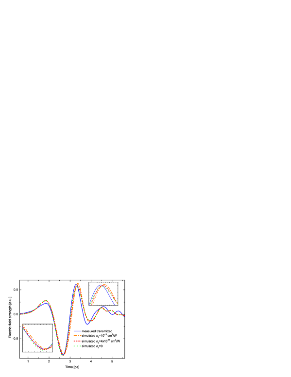
Figure 6: Comparison of transmitted and simulated results for different values of nonlinear index of refraction assuming uniform transverse distribution.

In order to model diffraction effects we take the incoming pulse with a Gaussian transverse profile and for the measured values of reference and transmitted field take an average over the width of diameter $D\approx 1\;$mm corresponding to the experimental condition. Using the estimated value of the width parameter $a_{r}\approx 0.6\;$mm shows marked improvement of agreement with measurement for the first oscillation and brings the preferred value of the nonlinear index of refraction to around $10^{-11}\;\mbox{cm}^{2}$/W as shown in figure 7. One has to acknowledge that the relatively small size of the nonlinear effect for the studied intensity and propagation distance introduces considerable uncertainty in that estimate and for more precise determination dedicated experiments with larger intensity and/or propagation distance would be required. In case of longer propagation distances surpassing the attenuation length a more careful consideration of attenuative dispersion would be required as shown by results obtained in [21, 29].

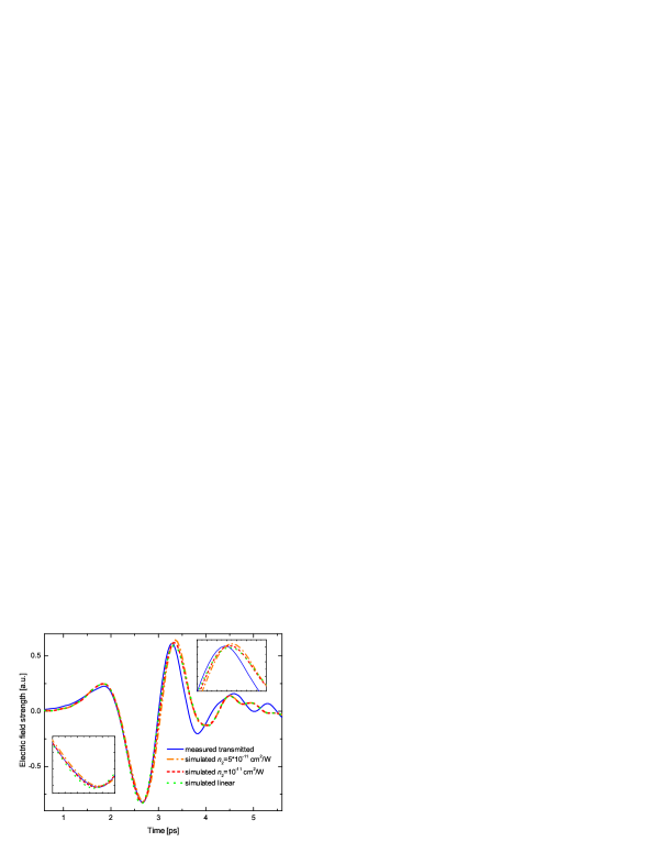
Figure 7: Comparison of transmitted and simulated results for different values of nonlinear index of refraction for Gaussian transverse profile of incoming beam with $a_{r}=0.6\;$mm.

We also investigated the influence of frequency-dependent absorption coefficient slowly increasing with frequency motivated by results of [32] but since it did not produce noticeable change in the agreement with observation we only show results for the constant value of $\alpha=1\;$cm^-1.

4 Conclusions

We studied diffraction effects during nonlinear propagation of few-cycle light pulses with axial symmetry in the framework of unidirectional propagation equation derived for the case of weak dispersion by suitably modified factorization method not relying on the paraxial approximation. The slowly-evolving-wave approximation is obtained as a special case and numerical simulations show similar results with significant differences present in case of high intensity accompanied with pronounced self focusing effects. Analysis of short terahertz pulse propagation in LiNbO₃ shows both nonlinear and diffraction effects despite of short propagation distance and indicates presence of a Kerr-type nonlinearity with nonlinear index of refraction $n_{2}\approx 10^{-11}\;\mbox{cm}^{2}$/W which is three orders of magnitude larger than its value in the visible part of spectrum. This points to significant contribution of lattice vibration anharmonicity and indicates pronounced suitability of terahertz pulses for investigating nonlinear lattice dynamics.

References

References

- [1] Brabec T and Krausz F 1997 Phys. Rev. Lett. 78 3282–3285
- [2] Ranka J K and Gaeta A L 1998 Opt. Lett. 23 534–536
- [3] Porras M A 1999 Phys. Rev. A 60 5069–5073
- [4] Gaeta A L 2002 Opt. Lett. 27 924–926
- [5] Tarasishin A V, Magnitskii S A and Zheltikov A M 2001 Opt. Comm. 193 187–196
- [6] Kolesik M, Moloney J V and Mlejnek M 2002 Phys. Rev. Lett. 89 283902
- [7] Kolesik M and Moloney J V 2004 Phys. Rev. E 70 036604
- [8] Kinsler P and New G H C 2003 Phys. Rev. A 67 023813
- [9] Kinsler P, Radnor S B P and New G H C 2005 Phys. Rev. A 72 063807
- [10] Kinsler P 2010 Phys. Rev. A 81 013819
- [11] Kinsler P 2010 Phys. Rev. A 81 023808
- [12] Kovachev L M 2007 Opt. Exp. 15 10318–10323
- [13] Belyaeva T J, Serkin V N, Aguero M A, Hernandez-Tenorio C and Kovachev L M 2011 Laser Physics 21 258–263
- [14] Kovachev L M and Georgieva D A 2013 Proc. SPIE 8770 87701G–87701G–10
- [15] Kovachev L M, Georgieva D A and Serkin V N 2013 AIP Conf. Proc. 1561 289
- [16] Kovachev L M 2014 AIP Conf. Proc. 1629 167
- [17] Rothenberg J E 1992 Opt. Lett. 17 1340–1342
- [18] Ferrando A, Zacares M, de Cordoba P F, Binosi D and Montero A 2005 Phys. Rev. E 71 016601
- [19] Haykin S Communication Systems (John Wiley, New York, 2001)
- [20] Conforti M, Baronio F and Angelis C D 2010 Phys. Rev. A 81 053841
- [21] Xiao H and Oughstun K E 1999 J. Opt. Soc. Am. B 16 1773–1785
- [22] Oughstun K E Electromagnetic and Optical Pulse Propagation 2: Temporal Pulse Dynamics in Dispersive, Attenuative Media (Springer, 2009)
- [23] Agrawal G P Nonlinear Fiber Optics (Academic Press, Oxford, 2013)
- [24] Jackson J D Classical Electrodynamics (John Wiley & Sons, New York, 1999)
- [25] Lalor E 1968 J. Opt. Soc. Am. 58 1235–1237
- [26] Sherman G C 1968 Phys. Rev. Lett. 21 761–764
- [27] Sherman G C 1969 J. Opt. Soc. Am. 59 697–711
- [28] Kitamura R, Pilon L and Jonasz M 2007 Appl. Phys. B 46 8118–8133
- [29] Palombini C L and Oughstun K E 2010 Opt. Exp. 18 23104–23120
- [30] Lenzner M, Kruger J, Sartania S, Cheng Z, Spielmann C, Mourou G, Kautek W and Krausz F 1998 Phys. Rev. Lett. 80 4076–4079
- [31] Hebling J, Hoffmann M C, Yeh K L, Tóth G and Nelson K A 2009 Nonlinear lattice response observed through terahertz spm Ultrafast Phenomena XVI ed Corkum P, DeSilvestri S, Nelson K and Reidle E (Springer-Verlag) pp 651–653
- [32] Pálfalvi L, Hebling J, Kuhl J, Péter A and Polgár K 2005 J. Appl. Phys. 97 123505
- [33] Unferdorben M, Szaller Z, Hajdara I, Hebling J and Pálfalvi L 2015 J. Infrared Milli. Terahz. Waves DOI 10.1007/s10762–015–0165–5
- [34] Seres J and Hebling J 2000 J. Opt. Soc. Am. B 17 741–750
- [35] Hebling J, Yeh K L, Hoffmann M C, Bartal B and Nelson K A 2008 J. Opt. Soc. Am. B 25 6–19
- [36] Sutherland R L Handbook of Nonlinear Optics (Marcel Dekker, New York, 2003)