On the Convergence of Stochastic Variational Inference in Bayesian Networks

Abstract

We highlight a pitfall when applying stochastic variational inference to general Bayesian networks. For global random variables approximated by an exponential family distribution, natural gradient steps, commonly starting from a unit length step size, are averaged to convergence. This useful insight into the scaling of initial step sizes is lost when the approximation factorizes across a general Bayesian network, and care must be taken to ensure practical convergence. We experimentally investigate how much of the baby (well-scaled steps) is thrown out with the bath water (exact gradients).

1 Introduction

Stochastic variational inference is framed as maximizing a global variational parameter $\mathbf{\Lambda}$, which is the natural parameter of a conjugate exponential distribution [2]. In this framework, stochastic gradient steps are taken along the natural gradient [1] to optimize for $\mathbf{\Lambda}$. A pleasing property of stochastic variational inference on a conjugate exponential distribution and approximation $q(\mathbf{\Lambda})$ is that the gradient is automatically rescaled so that a unit-length step size will minimize it. For a general Bayesian network, where the global variational parameters are subdivided to parameterize different factors $q_{i}$ in the network’s variational approximation, the picture is less clear. Hoffman et al.’s appendix suggests a stochastic updating scheme like that of the global version [2]. We show here that the problem is more subtle in the general case, as component-wise noisy natural gradients can tightly couple variational parameters, and following the default recipe can sometimes lead to a scheme that “diverges” beyond recovery!

These remarks are of particular value to the Xbox recommender system, which uses stochastic variational inference in a Bayesian network on “worldwide” scale [4, 5]. Some of the results presented in Sec. 3 are preliminary investigations that were done when designing the system in 2012.

2 Variational Bayes

A Bayesian network between the variables $\mathbf{X}=\{\mathbf{x}_{j}\}$ defines the conditional dependency structure between them through their joint probability $p(\mathbf{X})=\prod_{j}p(\mathbf{x}_{j}|\mathrm{pa}_{j})$. Following Fig. 1, let $\mathrm{pa}(j)$ be the set of indexes of parents of random variable(s) $\mathbf{x}_{j}$; for notational convenience we let $\mathrm{pa}_{j}\stackrel{{\scriptstyle.}}{{=}}\{\mathbf{x}_{k}:k\in\mathrm{pa}(j)\}$ denote the parent variables. The variables in the network can be hidden or observed, $\mathbf{X}=\{\mathbf{X}^{\mathrm{h}},\mathbf{X}^{\mathrm{o}}\}$. Variational Bayes (VB) approximates the posterior $p(\mathbf{X}^{\mathrm{h}}|\mathbf{X}^{\mathrm{o}})$ with $q(\mathbf{X}^{\mathrm{h}})$, by maximizing the evidence lower bound

$$\mathcal{L}[q]\stackrel{{\scriptstyle.}}{{=}}\int q(\mathbf{X}^{\mathrm{h}})\log\frac{p(\mathbf{X})}{q(\mathbf{X}^{\mathrm{h}})}\,\mathrm{d}\mathbf{X}^{\mathrm{h}}\leq\log p(\mathbf{X}^{\mathrm{o}})\ .$$

If $i$ indexes the hidden variables, we factorize the approximation with

$$q(\mathbf{X}^{\mathrm{h}})=\prod_{i}q_{i}(\mathbf{x}_{i})\ .$$

Let $\mathbb{E}_{j\neq i}$ indicate the expectation taken over $\prod_{j\neq i}q_{j}(\mathbf{x}_{j})$. The bound can be maximized in a component-wise fashion by iteratively setting each $q_{i}(\mathbf{x}_{i})$ to the maximum

$$\log q_{i}^{*}(\mathbf{x}_{i})=\mathbb{E}_{j\neq i}\Big{[}\log p(\mathbf{x}_{i}|\mathrm{pa}_{i})\Big{]}+\sum_{k\in\mathrm{ch}(i)}\mathbb{E}_{j\neq i}\Big{[}\log p(\mathbf{x}_{k}|\mathrm{pa}_{k})\Big{]}+\mathop{\rm const}\ .$$ (1)

In many practical networks there are some $\mathbf{x}_{i}$ for which number of children $N_{i}\stackrel{{\scriptstyle.}}{{=}}|\mathrm{ch}(i)|$ is large. In [2], $\mathbf{x}_{i}$ is a topic-vocabulary distribution from which millions of documents are generated. In Sec. 3 and [4, 5] the interaction is bilinear, where user $\mathbf{x}_{i}$ and item $\mathbf{x}_{j}$ variables are combined to represent a user’s affinity to an item. Rather than summing over all $\mathrm{ch}(i)$ for each update in (1), we aim to stochastically approximate the expectations. It alleviates two problems: firstly, the sum contains many terms; secondly, the update depends on some $q(\mathbf{x}_{j})$ which will be re-estimated, and the expense of fully estimating $q(\mathbf{x}_{i})$ is lost as it too will be re-estimated.

Figure 1: A Bayesian network, indicating $\mathbf{x}_{i}$’s Markov blanket. The parents of $\mathbf{x}_{i}$ are $\mathrm{pa}_{i}$ and its children $\mathbf{x}_{k}\in\mathrm{ch}_{i}$. For a compact notation we also write $k\in\mathrm{ch}(i)$ as the index set of children, where it is clear from context. Each child $k$ has parents $\mathbf{x}_{i}$ and $\mathrm{cp}_{i}$ (the co-parents with $\mathbf{x}_{i}$). The form of our notation loosely matches Winn and Bishop’s in [6], as Alg. 1 can be interpreted as “stochastic variational message passing”.

2.1 Conditionally conjugate models

The updates in (1) are straightforward when the Bayesian network is conditionally conjugate; that is, when the distribution of $\mathbf{x}_{i}$, conditioned on $\mathrm{pa}_{i}$, is (a) drawn from an exponential family, and (b) is conjugate with respect to the distribution of $\mathrm{pa}_{i}$. We define the exponential family as

$$\log p(\mathbf{x}_{i}|\mathrm{pa}_{i})=\bm{\eta}_{i}(\mathrm{pa}_{i})^{T}\phi_{i}(\mathbf{x}_{i})+f_{i}(\mathbf{x}_{i})+g_{i}(\mathrm{pa}_{i})$$ (2)

where $\bm{\eta}_{i}(\mathrm{pa}_{i})$ is the natural parameter vector, $\phi_{i}(\mathbf{x}_{i})$ forms the sufficient statistics, and $g_{i}(\mathrm{pa}_{i})$ defines the normalizing constant through $g_{i}(\mathrm{pa}_{i})=-\log\int\exp\{\bm{\eta}_{i}(\mathrm{pa}_{i})^{T}\phi_{i}(\mathbf{x}_{i})+f_{i}(\mathbf{x}_{i})\}\,\mathrm{d}\mathbf{x}_{i}$. We can view (2) as a “prior” over $\mathbf{x}_{i}$. Now consider a node $\mathbf{x}_{k}\in\mathrm{ch}_{i}$ in Fig. 1. We subdivide $\mathrm{pa}_{k}$, the parents of $\mathbf{x}_{k}$, into $\mathbf{x}_{i}$ and its co-parents $\mathrm{cp}_{i}$:

$$\log p(\mathbf{x}_{k}|\mathbf{x}_{i},\mathrm{cp}_{i})=\bm{\eta}_{k}(\mathbf{x}_{i},\mathrm{cp}_{i})^{T}\phi_{k}(\mathbf{x}_{k})+f(\mathbf{x}_{k})+g(\mathbf{x}_{i},\mathrm{cp}_{i})\ .$$

We can view this as a contribution to the “likelihood” of $\mathbf{x}_{i}$. We include the co-parents as they are part of $\mathbf{x}_{i}$’s Markov blanket. Through conjugacy, $p(\mathbf{x}_{i}|\mathrm{pa}_{i})$ and $p(\mathbf{x}_{k}|\mathbf{x}_{i},\mathrm{cp}_{i})$ have the same functional form with respect to $\mathbf{x}_{i}$, so that we can rewrite $p(\mathbf{x}_{k}|\mathbf{x}_{i},\mathrm{cp}_{i})$ in terms of the sufficient statistics $\phi_{i}(\mathbf{x}_{i})$ by defining some function $\bm{\eta}_{ki}$ with

$$\log p(\mathbf{x}_{k}|\mathbf{x}_{i},\mathrm{cp}_{i})=\bm{\eta}_{ki}(\mathbf{x}_{k},\mathrm{cp}_{i})^{T}\phi_{i}(\mathbf{x}_{i})+h(\mathbf{x}_{k},\mathrm{cp}_{i})\ .$$

We furthermore parameterize the $q(\mathbf{x}_{i})$ distributions in terms of their natural parameters. To distinguish them, we denote their natural parameters by $\bm{\lambda}_{i}$, and define $\mathbf{\Lambda}\stackrel{{\scriptstyle.}}{{=}}[\bm{\lambda}_{1},\ldots,\bm{\lambda}_{I}]$:

$$\log q_{i}(\mathbf{x}_{i}|\bm{\lambda}_{i})=\bm{\lambda}_{i}^{T}\phi_{i}(\mathbf{x}_{i})+f_{i}(\mathbf{x}_{i})+\tilde{g}_{i}(\bm{\lambda}_{i})\ .$$ (3)

2.2 Variational Bayes updates and their stochastic version

Returning to (1), we can write

$$\log q_{i}^{*}(\mathbf{x}_{i})=\mathbb{E}_{j\neq i}\Bigg{[}\bm{\eta}_{i}(\mathrm{pa}_{i})+\sum_{k\in\mathrm{ch}(i)}\bm{\eta}_{ki}(\mathbf{x}_{k},\mathrm{cp}_{i})\Bigg{]}^{T}\phi_{i}(\mathbf{x}_{i})+f_{i}(\mathbf{x}_{i})+\mathop{\rm const}\ ,$$ (4)

from which we can directly read off the updated natural parameter $\bm{\lambda}_{i}^{*}$ through (3). Notice now that $\bm{\eta}_{i}$ is a multi-linear function of the random variables $\mathrm{pa}_{i}$, i.e. it is linear in each parent random variable. In the same way $\bm{\eta}_{ki}$ is a multi-linear function of the random variables $\mathbf{x}_{k}$ and $\mathrm{cp}_{i}$. Furthermore, $q$ factorizes over these variables (except where they are observed, of course). We can therefore reparameterize (4) in terms of expectations over $q_{j}$, $i\neq j$ with

$$\mathbb{E}_{j\neq i}\Big{[}\bm{\eta}_{i}(\mathrm{pa}_{i})\Big{]} =\widetilde{\bm{\eta}}_{i}\left(\Big{\{}\mathbb{E}_{j}\Big{[}\phi_{j}(\mathbf{x}_{j})\Big{]}\Big{\}}_{j\in\mathrm{pa}(i)}\right)\stackrel{{\scriptstyle.}}{{=}}\widetilde{\bm{\eta}}_{i}$$

$$\mathbb{E}_{j\neq i}\Big{[}\bm{\eta}_{ki}(\mathbf{x}_{k},\mathrm{cp}_{i})\Big{]} =\widetilde{\bm{\eta}}_{ki}\left(\mathbb{E}_{k}\Big{[}\phi_{k}(\mathbf{x}_{k})\Big{]},\,\Big{\{}\mathbb{E}_{j}\Big{[}\phi_{j}(\mathbf{x}_{j})\Big{]}\Big{\}}_{j\in\mathrm{cp}(i)}\right)\stackrel{{\scriptstyle.}}{{=}}\widetilde{\bm{\eta}}_{ki}\ .$$

1:  for $t=1$ to $t_{\max}$ or convergence do

2:     $\rho_{t}=(t+\tau)^{-\kappa}$

3:     for each hidden $\mathbf{x}_{i}$ do

4:        $\mathcal{C}\leftarrow C$ random nodes from $\mathrm{ch}_{i}$

5:        $\bm{\lambda}_{i}^{\mathrm{temp}}\leftarrow\widetilde{\bm{\eta}}_{i}+\frac{N_{i}}{C}\sum_{k\in\mathcal{C}}\widetilde{\bm{\eta}}_{ki}$

6:        option (a): $\bm{\lambda}_{i}\leftarrow(1-\rho_{t})\bm{\lambda}_{i}+\rho_{t}\bm{\lambda}_{i}^{\mathrm{temp}}$

7:     end for

8:     option (b): $\mathbf{\Lambda}\leftarrow(1-\rho_{t})\mathbf{\Lambda}+\rho_{t}\mathbf{\Lambda}^{\mathrm{temp}}$

9:  end for

Algorithm 1 Stochastic Variational Bayes

This is a key ingredient of algorithms like variational message passing [6]. (When $\mathbf{x}_{k}$ is observed, $\phi_{k}(\mathbf{x}_{k})$ is kept as is, as it is averaged over a delta function.) The variational update in (4) becomes

$$\bm{\lambda}_{i}^{*}=\widetilde{\bm{\eta}}_{i}+\sum_{k\in\mathrm{ch}(i)}\widetilde{\bm{\eta}}_{ki}\ .$$ (5)

The update is a step along the natural gradient [1], equivalent to setting the gradient to zero by solving for the zero of the derivative of $\mathcal{L}$ with respect to $\bm{\lambda}_{i}$. In particular, (5) updates $\bm{\lambda}_{i}$ from its old value to $\bm{\lambda}_{i}^{*}$ using a step of unit length along the natural gradient. Sec. A.1 derives the gradient $\nabla_{\bm{\lambda}_{i}}\mathcal{L}$, and Sec. A.2 states its natural form $\widehat{\nabla}_{\bm{\lambda}_{i}}\mathcal{L}$.

When $N_{i}\stackrel{{\scriptstyle.}}{{=}}|\mathrm{ch}(i)|$ is large, not all the child nodes might be accessed in reasonable time. Furthermore, when $q(\mathbf{x}_{i})$ is re-estimated, the (previous) large computation is discarded and recomputed. We may alternatively consider a subsample of nodes from $\mathrm{ch}(i)$ to determine the sufficient statistics. By placing a uniform distribution $\widetilde{p}_{i}$ on the atoms $\widetilde{\bm{\eta}}_{ki}$, the update from (5) is equivalent to $\bm{\lambda}_{i}=\widetilde{\bm{\eta}}_{i}+N_{i}\,\mathbb{E}_{\widetilde{p}_{i}}[\widetilde{\bm{\eta}}]$. This expectation can be estimated in many ways. Let set $\mathcal{C}$ be a sample of $C$ children from $\mathrm{ch}_{i}$ without replacement and let

$$\bm{\lambda}_{i}^{\mathrm{temp}}=\widetilde{\bm{\eta}}_{i}+\frac{N_{i}}{C}\sum_{k\in\mathcal{C}}\widetilde{\bm{\eta}}_{ki}\ .$$ (6)

Taking expectations gives $\bm{\lambda}_{i}^{*}=\mathbb{E}[\bm{\lambda}_{i}^{\mathrm{temp}}]=\widetilde{\bm{\eta}}_{i}+N_{i}\mathbb{E}_{\widetilde{p}_{i}}[\widetilde{\bm{\eta}}]$. With $\rho_{t}\to 0$, $\sum_{t=1}^{\infty}\rho_{t}=\infty$ and $\sum_{t=1}^{\infty}\rho_{t}^{2}<\infty$, these stochastic natural gradients are used in Alg. 1, which is a stochastic version of variational message passing. In Alg. 1, scalar $\kappa\in(\frac{1}{2},1]$ is a forgetting rate, while delay $\tau\geq 0$ discounts early iterations more.

There are two options in Alg. 1. For option (a), the mean value of the parameters of $q(\mathbf{X}^{\mathrm{h}})$ is periodic in $I$, the number of factors in $q$, and convergence to a local optimum can also be guaranteed for $I$-dependent mean values [3]. Option (b) is the update scheme given in [2].

3 Bayesian matrix factorization

To illustrate a general Bayesian network, we factorize a sparse matrix of a subsample of a million entries in the Netflix data set ($M=4805$ users and $N=16015$ items). Each entry $r_{mn}$ is user $m$’s rating of movie $n$ on a five-star rating scale. For illustrative purposes, consider a Gaussian bilinear ratings model

$$p(r_{mn}|\mathbf{u}_{m},\mathbf{v}_{n})=\mathcal{N}(r_{mn}\,;\,\mathbf{u}_{m}^{T}\mathbf{v}_{n},\,1)$$

for user parameter vector $\mathbf{u}_{m}\in\mathbb{R}^{K}$ and item trait vector $\mathbf{v}_{n}\in\mathbb{R}^{K}$. We place a factorized prior $\mathcal{N}(u_{mk}\,;\,0,1)$ on each of the entries of $\mathbf{u}_{m}$ and $\mathbf{v}_{n}$. We choose a fully factorized Gaussian approximation $q(\mathbf{U})=\prod_{m}\prod_{k}q(u_{mk})$, with a similar approximation for $q(\mathbf{V})$. The VB update for $q(u_{mk})$ therefore incorporates $2K-1$ co-parents due to the inner product. With the Gaussian’s natural parameters being its precision and mean-times-precision, it is

$$\bm{\lambda}_{mk}^{\mathrm{temp}}=\begin{pmatrix}\mathsf{prec}\\ \mathsf{mean}\cdot\mathsf{prec}\end{pmatrix}=\begin{pmatrix}1\\ 0\end{pmatrix}+\frac{N_{m}}{C}\sum_{n\in\mathcal{C}}\begin{pmatrix}\mathop{\sf var}_{q}[v_{nk}]+\mathbb{E}_{q}[v_{nk}]^{2}\\ \mathbb{E}_{q}[v_{nk}](r_{mn}-\sum_{k^{\prime}\neq k}\mathbb{E}_{q}[u_{mk^{\prime}}]\mathbb{E}_{q}[v_{nk^{\prime}}])\end{pmatrix}\ .$$ (7)

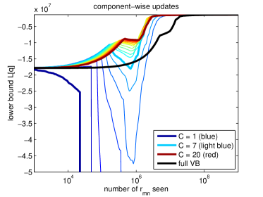
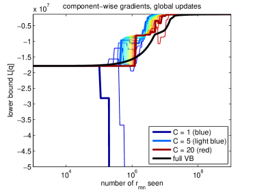
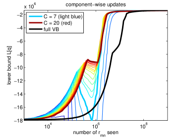
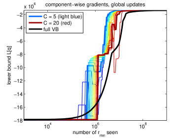
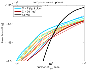
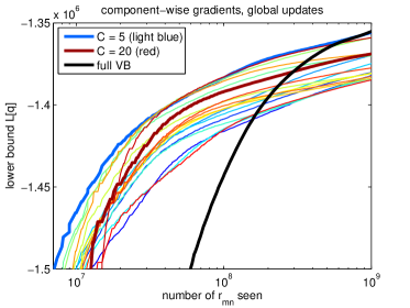
Figure 2: Convergence of ${\cal L}[q]$ with $\rho_{t}=t^{-0.6}$. Alg. 1’s option (a) is shown in the left column; option (b) is shown in the right column. The x-axes are on a logarithmic scale. The global stochastic gradient is not in its natural form, and the effect of a large variance in the gradient estimate and overshooting with too large step sizes of $\rho_{t}\in(0,1]$ is clearly visible for small $C$. Note that $r_{mn}$’s can be revisited over multiple loops in Alg. 1. Different magnifications of the same two convergence plots for options (a) and (b) are shown in the three rows of graphs.

Fig. 2 shows ${\cal L}[q]$ as a function of the number of times that individual ratings (observed nodes) $r_{mn}$ are accessed or queried (using $K=5$). The value of the bound is shown for the use of at most $C=1,\ldots,20$ children when estimating the gradient of each random variable with (6) and (7). Both options (a) and (b) in Alg. 1 “diverge” in a numerically unrecoverable way when $C$ is small. This is due to the global gradient not being in its natural form, and using a step size of $\rho_{t}\in(0,1]$ that is too big, overshooting with too large gradient steps.

Full VB, shown in black in Fig. 2, implicitly uses $\rho_{t}=1$ in (5). As the stochastic natural gradient depends on other $\bm{\lambda}_{j}$, much smaller initial step sizes are required to not “overshoot”. The variance of the gradient is simply too large compared to $\rho_{t}$. Fig. 2 illustrates this problem for general Bayesian networks; see especially the top left figure.

In practice, we can overcome this problem overcome by starting with sufficiently small initial step sizes $\rho_{t}\ll 1$. For $C=1$ in option (a) this was starting from $\rho_{1}=\frac{1}{512}$, and $\rho_{1}=\frac{1}{64}$ for option (b). In [4, 5] the value of $C$ varied depending on a user or item’s usage, and there $\rho_{t}=1$ was fixed for the first ten iterations before slowly decreasing it.

Have we thrown the baby (well-scaled steps) out with the bath water (exact gradients)? Maybe some. As shown by this short note, it is still an open question.

Appendix A Gradients

In this Appendix, we derive the component-wise gradients and their natural version, and present basic intuition for why steps down the stochastic gradient can be taken.

A.1 Component-wise gradients

The function that’s minimized to find (5) is $\mathcal{L}(\bm{\lambda}_{i})$ below. It is a function of $\bm{\lambda}_{i}$, whilst keeping all other $\bm{\lambda}_{j}$ for $j\neq i$ fixed:

$$\mathcal{L}(\bm{\lambda}_{i}) =\mathbb{E}_{q}\Bigg{[}\log p(\mathbf{x}_{i}|\mathrm{pa}_{i})+\sum_{k\in\mathrm{ch}(i)}\log p(\mathbf{x}_{k}|\mathbf{x}_{i},\mathrm{cp}_{i})-\log q_{i}(\mathbf{x}_{i}|\bm{\lambda}_{i})\Bigg{]}$$

$$=\mathbb{E}_{q}\Bigg{[}\bm{\eta}_{i}(\mathrm{pa}_{i})^{T}\phi_{i}(\mathbf{x}_{i})+f_{i}(\mathbf{x}_{i})+g_{i}(\mathrm{pa}_{i})$$

$$\qquad\qquad+\sum_{k\in\mathrm{ch}(i)}\Big{(}\bm{\eta}_{k}(\mathbf{x}_{i},\mathrm{cp}_{i})^{T}\phi_{k}(\mathbf{x}_{k})+f(\mathbf{x}_{k})+g(\mathbf{x}_{i},\mathrm{cp}_{i})\Big{)}$$

$$\qquad\qquad-\bm{\lambda}_{i}^{T}\phi_{i}(\mathbf{x}_{i})-f_{i}(\mathbf{x}_{i})-\tilde{g}_{i}(\bm{\lambda}_{i})\Bigg{]}$$

Because of local conjugacy, $p(\mathbf{x}_{k}|\mathbf{x}_{i},\mathrm{cp}_{i})$ can be rewritten in terms of the sufficient statistics $\phi_{i}(\mathbf{x}_{i})$ through a multi-linear function $\bm{\eta}_{ki}$ of the random variables $\mathbf{x}_{k}$ and $\mathrm{cp}_{i}$ to yield

$$\mathcal{L}(\bm{\lambda}_{i}) =\mathbb{E}_{q}\Bigg{[}\bm{\eta}_{i}(\mathrm{pa}_{i})^{T}\phi_{i}(\mathbf{x}_{i})+f_{i}(\mathbf{x}_{i})+g_{i}(\mathrm{pa}_{i})+\sum_{k\in\mathrm{ch}(i)}\Big{(}\bm{\eta}_{ki}(\mathbf{x}_{k},\mathrm{cp}_{i})^{T}\phi_{i}(\mathbf{x}_{i})+h(\mathbf{x}_{k},\mathrm{cp}_{i})\Big{)}$$

$$\qquad\qquad-\bm{\lambda}_{i}^{T}\phi_{i}(\mathbf{x}_{i})-f_{i}(\mathbf{x}_{i})-\tilde{g}_{i}(\bm{\lambda}_{i})\Bigg{]}\ .$$

Taking expectations over $q$ gives, as function of $\bm{\lambda}_{i}$,

$$\mathcal{L}(\bm{\lambda}_{i})=\Bigg{(}\widetilde{\bm{\eta}}_{i}+\sum_{k\in\mathrm{ch}(i)}\widetilde{\bm{\eta}}_{ki}\Bigg{)}^{T}\mathbb{E}_{i}\left[\phi_{i}(\mathbf{x}_{i})\right]-\bm{\lambda}_{i}^{T}\mathbb{E}_{i}\left[\phi_{i}(\mathbf{x}_{i})\right]-\tilde{g}_{i}(\bm{\lambda}_{i})+\mathrm{const}\ ,$$ (8)

with $\tilde{g}_{i}(\bm{\lambda}_{i})=-\log\int\exp\{\bm{\lambda}_{i}^{T}\phi_{i}(\mathbf{x}_{i})+f_{i}(\mathbf{x}_{i})\}\,\mathrm{d}\mathbf{x}_{i}$. The derivatives of the log partition function $-\tilde{g}_{i}(\bm{\lambda}_{i})$ with respect to $\bm{\lambda}_{i}$ give the expected sufficient statistics

$$-\nabla\tilde{g}_{i}(\bm{\lambda}_{i}) =\mathbb{E}_{i}\left[\phi_{i}(\mathbf{x}_{i})\right]$$

$$-\nabla^{2}\tilde{g}_{i}(\bm{\lambda}_{i}) =\nabla\mathbb{E}_{i}\left[\phi_{i}(\mathbf{x}_{i})\right]$$

$$=\mathbb{E}_{i}\left[\Big{(}\phi_{i}(\mathbf{x}_{i})-\mathbb{E}_{i}\left[\phi_{i}(\mathbf{x}_{i})\right]\Big{)}\Big{(}\phi_{i}(\mathbf{x}_{i})-\mathbb{E}_{i}\left[\phi_{i}(\mathbf{x}_{i})\right]\Big{)}^{T}\right]$$

$$={\sf cov}_{i}\left[\phi_{i}(\mathbf{x}_{i})\right]\ ,$$

and by using properties of the exponential family, the gradient of $\mathcal{L}$ with respect to $\bm{\lambda}_{i}$ is therefore

$$\nabla_{\bm{\lambda}_{i}}\mathcal{L}(\bm{\lambda}_{i})={\sf cov}_{i}\left[\phi_{i}(\mathbf{x}_{i})\right]\Bigg{(}\widetilde{\bm{\eta}}_{i}+\sum_{k\in\mathrm{ch}(i)}\widetilde{\bm{\eta}}_{ki}-\bm{\lambda}_{i}\Bigg{)}\ .$$ (9)

Solving for $\nabla_{\bm{\lambda}_{i}}\mathcal{L}(\bm{\lambda}_{i})=\mathbf{0}$ yields the component-wise VB update $\bm{\lambda}_{i}^{*}=\widetilde{\bm{\eta}}_{i}+\sum_{k\in\mathrm{ch}(i)}\widetilde{\bm{\eta}}_{ki}$ that we find in (5). Gradient $\nabla_{\bm{\lambda}_{i}}\mathcal{L}$ depends on $\bm{\lambda}_{i}$ through ${\sf cov}_{i}[\phi_{i}(\mathbf{x}_{i})]$ and $\bm{\lambda}_{i}$, and in the next section we will show that the natural gradient $\widetilde{\nabla}_{\bm{\lambda}_{i}}\mathcal{L}$ removes the dependency on ${\sf cov}_{i}[\phi_{i}(\mathbf{x}_{i})]$, so that it is a linear function of $\bm{\lambda}_{i}$, with the minimum being attained by taking a step of length one along it.

A.2 Component-wise natural gradients

The Fisher information matrix of $q_{i}$ is

$$G(\bm{\lambda}_{i}) =\mathbb{E}_{i}\left[\Big{(}\nabla_{\bm{\lambda}_{i}}\log q(\mathbf{x}_{i}|\bm{\lambda}_{i})\Big{)}\Big{(}\nabla_{\bm{\lambda}_{i}}\log q(\mathbf{x}_{i}|\bm{\lambda}_{i})\Big{)}^{T}\right]$$

$$=\mathbb{E}_{i}\left[\Big{(}\phi_{i}(\mathbf{x}_{i})-\mathbb{E}_{i}[\phi_{i}(\mathbf{x}_{i})]\Big{)}\Big{(}\phi_{i}(\mathbf{x}_{i})-\mathbb{E}_{i}[\phi_{i}(\mathbf{x}_{i})]\Big{)}^{T}\right]$$

$$={\sf cov}_{i}\left[\phi_{i}(\mathbf{x}_{i})\right]\ ,$$

and the component-wise natural gradient is obtained by multiplying it with $\nabla_{\bm{\lambda}_{i}}\mathcal{L}$, yielding

$$\widehat{\nabla}_{\bm{\lambda}_{i}}\mathcal{L}(\bm{\lambda}_{i})\stackrel{{\scriptstyle.}}{{=}}G(\bm{\lambda}_{i})^{-1}\nabla_{\bm{\lambda}_{i}}\mathcal{L}(\bm{\lambda}_{i})\\ =\widetilde{\bm{\eta}}_{i}+\sum_{k\in\mathrm{ch}(i)}\widetilde{\bm{\eta}}_{ki}-\bm{\lambda}_{i}\ .$$

A gradient descent along the natural gradient is taken with step length $\rho>0$. Starting at point $\bm{\lambda}_{i}^{(t-1)}$, gradient descent updates it to $\bm{\lambda}_{i}^{(t)}$ with

$$\bm{\lambda}_{i}^{(t)}\leftarrow\bm{\lambda}_{i}^{(t-1)}+\rho\widehat{\nabla}_{\bm{\lambda}_{i}^{(t-1)}}\mathcal{L}(\bm{\lambda}_{i}) =\bm{\lambda}_{i}^{(t-1)}+\rho\Bigg{(}\widetilde{\bm{\eta}}_{i}+\sum_{k\in\mathrm{ch}(i)}\widetilde{\bm{\eta}}_{ki}-\bm{\lambda}_{i}^{(t-1)}\Bigg{)}$$

$$=(1-\rho)\bm{\lambda}_{i}^{(t-1)}+\rho\Bigg{(}\widetilde{\bm{\eta}}_{i}+\sum_{k\in\mathrm{ch}(i)}\widetilde{\bm{\eta}}_{ki}\Bigg{)}$$

$$=(1-\rho)\bm{\lambda}_{i}^{(t-1)}+\rho\bm{\lambda}_{i}^{*}\ .$$

When the above update is compared to (5), we see that the minimum $\bm{\lambda}_{i}^{(t)}\leftarrow\bm{\lambda}_{i}^{*}$ is obtained by applying a step size of $\rho=1$ along the natural gradient.

A.3 Stochastic natural gradients: a bird’s eye view

In this section an intuitive motivation will be provided for doing stochastic gradient descent using the natural gradient, as it was defined above in Sec. A.2. The explanation favours an intuitive understanding above mathematical rigour. Imagine that instead of $\bm{\lambda}_{i}^{*}$, we have access to a sequence of samples $\{\bm{\lambda}_{i}^{\mathrm{temp},\tau}\}_{\tau=1}^{t}$, so that $\mathbb{E}[\bm{\lambda}_{i}^{\mathrm{temp}}]=\bm{\lambda}_{i}^{*}$. We can write the update $\bm{\lambda}_{i}^{(t)}\leftarrow\bm{\lambda}_{i}^{*}$ recursively using the sample average

$$\bm{\lambda}_{i}^{(t)}\leftarrow\frac{1}{t}\sum_{\tau=1}^{t}\bm{\lambda}_{i}^{\mathrm{temp},\tau} =\left(1-\frac{1}{t}\right)\left(\frac{1}{t-1}\sum_{\tau=1}^{t-1}\bm{\lambda}_{i}^{\mathrm{temp},\tau}\right)+\frac{1}{t}\bm{\lambda}_{i}^{\mathrm{temp},t}$$

$$=\left(1-\frac{1}{t}\right)\bm{\lambda}_{i}^{(t-1)}+\frac{1}{t}\bm{\lambda}_{i}^{\mathrm{temp},t}\ .$$

Define $\rho_{t}\stackrel{{\scriptstyle.}}{{=}}\frac{1}{t}$. In the running average, $\sum_{t=1}^{\infty}\frac{1}{t}=\infty$ and $\sum_{t=1}^{\infty}\left(\frac{1}{t}\right)^{2}<\infty$, and therefore $\sum_{t=1}^{\infty}\rho_{t}=\infty$ and $\sum_{t=1}^{\infty}\rho_{t}^{2}<\infty$. In the running average with $\rho_{t}\stackrel{{\scriptstyle.}}{{=}}\frac{1}{t}$, each gradient sample is treated equally. However, instead of incorporating fraction $\frac{1}{t}$ of $\bm{\lambda}_{i}^{\mathrm{temp},t}$ into the running average, we may erase a bit more from the “past memory” $\bm{\lambda}_{i}^{(t-1)}$ to include a bit more of the recent gradient $\bm{\lambda}_{i}^{\mathrm{temp},t}$. How much more is permissible?

Now define $\rho_{t}\stackrel{{\scriptstyle.}}{{=}}t^{-\kappa}$. For $\kappa=\frac{1}{2}$, the previous samples will be forgotten at a faster rate, and more of $\bm{\lambda}_{i}^{\mathrm{temp},t}$ will be included through $\bm{\lambda}_{i}^{(t)}\leftarrow(1-t^{-1/2})\bm{\lambda}_{i}^{(t-1)}+t^{-1/2}\bm{\lambda}_{i}^{\mathrm{temp},t}$. However, at this rate past samples are forgotten too quickly, as both $\sum_{t=1}^{\infty}t^{-1/2}=\infty$ and $\sum_{t=1}^{\infty}(t^{-1/2})^{2}=\infty$. For any $\kappa^{\prime}>1$, both infinite sums will be finite, e.g. $\sum_{t=1}^{\infty}t^{-\kappa^{\prime}}<\infty$ and $\sum_{t=1}^{\infty}(t^{-\kappa^{\prime}})^{2}<\infty$, and the running average will cling on to old memories, and has too little capacity to incorporate recent gradient samples $\bm{\lambda}_{i}^{\mathrm{temp},t}$. Between forgetting too quickly or not at all, a setting of $\kappa\in(\frac{1}{2},1]$ in $\rho_{t}\stackrel{{\scriptstyle.}}{{=}}t^{-\kappa}$ is therefore permissible.

A.4 Converging with fickle neighbours

The running average in Sec. A.3 can boldly start at $\rho_{t}\stackrel{{\scriptstyle.}}{{=}}t^{-\kappa}=1$ for $t=1$, and from this unit length step along the natural gradient, accumulate gradient samples until convergence. However, it rests on the premise that neighbours $\bm{\lambda}_{j}$ for $j\neq i$ from the Markov blanket of $\mathbf{x}_{i}$ remain unchanged.

If this premise does not hold, much smaller steps $\rho_{t}\stackrel{{\scriptstyle.}}{{=}}(t+\tau)^{-\kappa}$ with delay $\tau\geq 0$ are required. This is indeed the case. As Sec. 3 shows, a delay $\tau\geq 0$ that is sufficiently large for the stochastic gradient scheme to converge in practice is not known a priori. By explicitly stating the shorthand definitions of $\widetilde{\bm{\eta}}_{i}$ and $\widetilde{\bm{\eta}}_{ki}$ in (8), it is clear that the other $\bm{\lambda}_{j}$ appear through multi-linear functions in

$$\mathcal{L}(\bm{\lambda}_{i}) =\left(\widetilde{\bm{\eta}}_{i}\Big{(}\big{\{}\mathbb{E}_{j}[\phi_{j}(\mathbf{x}_{j})]\big{\}}_{j\in\mathrm{pa}(i)}\Big{)}+\sum_{k\in\mathrm{ch}(i)}\widetilde{\bm{\eta}}_{ki}\Big{(}\mathbb{E}_{k}[\phi_{k}(\mathbf{x}_{k})],\,\big{\{}\mathbb{E}_{j}[\phi_{j}(\mathbf{x}_{j})]\big{\}}_{j\in\mathrm{cp}(i)}\Big{)}\right)^{T}\mathbb{E}_{i}\left[\phi_{i}(\mathbf{x}_{i})\right]$$

$$\quad\quad-\bm{\lambda}_{i}^{T}\mathbb{E}_{i}\left[\phi_{i}(\mathbf{x}_{i})\right]-\tilde{g}_{i}(\bm{\lambda}_{i})+\mathrm{const}\ .$$

If we now consider the global gradient $\nabla_{\mathbf{\Lambda}}\mathcal{L}(\mathbf{\Lambda})=[\nabla_{\bm{\lambda}_{1}}\mathcal{L}(\bm{\lambda}_{1}),\ldots,\nabla_{\bm{\lambda}_{I}}\mathcal{L}(\bm{\lambda}_{I})]$, it is clear from the above form (multi-linear in all variables) that we can’t set the gradient to zero and solve for all $\mathbf{\Lambda}$ explicitly, as was done in (5). It is usually not even convex problem.

The gradient steps are along the global natural gradient. It is defined as

$$\widetilde{\nabla}_{\mathbf{\Lambda}}\mathcal{L}(\mathbf{\Lambda})\stackrel{{\scriptstyle.}}{{=}}G(\mathbf{\Lambda})^{-1}\nabla_{\mathbf{\Lambda}}\mathcal{L}(\mathbf{\Lambda})\ ,$$

with $G(\mathbf{\Lambda})$ being the Fisher information matrix of $q$,

$$G(\mathbf{\Lambda})=\mathbb{E}_{q}\left[\Big{(}\nabla_{\mathbf{\Lambda}}\log q(\mathbf{X}^{\mathrm{h}}|\mathbf{\Lambda})\Big{)}\Big{(}\nabla_{\mathbf{\Lambda}}\log q(\mathbf{X}^{\mathrm{h}}|\mathbf{\Lambda})\Big{)}^{T}\right]\ .$$

$G(\mathbf{\Lambda})$ is block-diagonal, as the covariance between $\phi_{i}(\mathbf{x}_{i})$ and $\phi_{j}(\mathbf{x}_{j})$ is zero for $i\neq j$, due to the factorization of $q$. Its inverse is therefore also block-diagonal, and the natural gradient has the form $\widetilde{\nabla}_{\mathbf{\Lambda}}\mathcal{L}(\mathbf{\Lambda})=[\widetilde{\nabla}_{\bm{\lambda}_{1}}\mathcal{L}(\bm{\lambda}_{1}),\ldots,\widetilde{\nabla}_{\bm{\lambda}_{I}}\mathcal{L}(\bm{\lambda}_{I})]$.

Appendix B Global batch samples

An alternative to Alg. 1 is to take a batch data sample $\mathcal{D}$ of $C_{\mathrm{global}}$ observed variables at the start of each iteration, and follow either each $\widetilde{\nabla}_{\bm{\lambda}_{i}}\mathcal{L}(\bm{\lambda}_{i})$ or $\widetilde{\nabla}_{\mathbf{\Lambda}}\mathcal{L}(\mathbf{\Lambda})$. This is outlined in Alg. 2.

1:  for $t=1$ to $t_{\max}$ or convergence do

2:     $\rho_{t}=(t+\tau)^{-\kappa}$

3:     $\mathcal{D}\leftarrow C_{\mathrm{global}}$ random nodes from $\mathbf{X}^{\mathrm{o}}$

4:     for each hidden $\mathbf{x}_{i}$ : $i\in\mathrm{pa}(\mathcal{D})$ do

5:        $\mathcal{D}_{i}\leftarrow\{\mathbf{x}_{k}\in\mathcal{D}\cap\mathrm{ch}_{i}\}$

6:        $\bm{\lambda}_{i}^{\mathrm{temp}}\leftarrow\widetilde{\bm{\eta}}_{i}+\frac{N_{i}}{|\mathcal{D}_{i}|}\sum_{k\in\mathcal{C}}\widetilde{\bm{\eta}}_{ki}$

7:        option (a): $\bm{\lambda}_{i}\leftarrow(1-\rho_{t})\bm{\lambda}_{i}+\rho_{t}\bm{\lambda}_{i}^{\mathrm{temp}}$

8:     end for

9:     // updates of $\mathrm{pa}_{i}$ etc.

10:     option (b): $\mathbf{\Lambda}\leftarrow(1-\rho_{t})\mathbf{\Lambda}+\rho_{t}\mathbf{\Lambda}^{\mathrm{temp}}$

11:  end for

Algorithm 2 Stochastic Variational Bayes

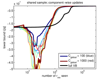
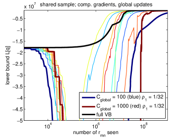
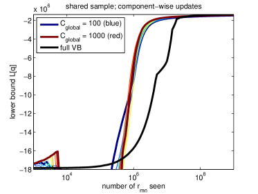
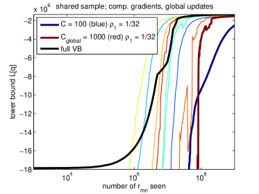
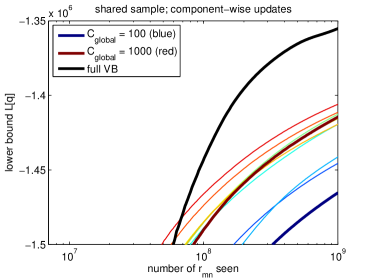
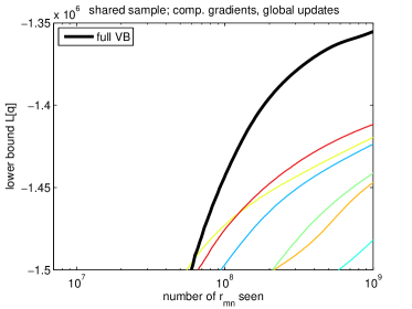
Figure 3: Convergence of ${\cal L}[q]$ with $\rho_{t}=t^{-0.6}$. Alg. 2’s option (a) is shown in the left column; option (b) is shown in the right column. The x-axes are on a logarithmic scale.

Fig. 3 considers batch sizes of $C_{\mathrm{global}}=100$ to 1000, in intervals of 100. The convergence in Fig. 3 is much slower than that of Fig. 2. For the global update in option (b) in Alg. 2, the algorithm only converged on finite machine precision when $\rho_{1}\leq\frac{1}{32}$ was chosen (smaller for some $C_{\mathrm{global}}$ settings), whereas for option (a) at least the algorithm converged from $\rho_{1}=1$ for all settings.

In Alg. 2, $\mathrm{pa}(\mathcal{D})$ is the set of hidden variables that have a child node in $\mathcal{D}$. Line 9 makes provision for updating variables (like hyper-parameters) that don’t have observed children; this was not required for our example.

References

- [1] S. Amari. Natural gradient works efficiently in learning. Neural Computation, 10(2):251–276, 1998.
- [2] M. D. Hoffman, D. M. Blei, C. Wang, and J. Paisley. Stochastic variational inference. Journal of Machine Learning Research, 14:1303–1347, 2013.
- [3] H. J. Kushner and G. G. Yin. Stochastic Approximation and Recursive Algorithms and Applications. Springer, 2003.
- [4] U. Paquet and N. Koenigstein. One-class collaborative filtering with random graphs. In Proceedings of the 22nd international conference on World Wide Web, WWW ’13, pages 999–1008, 2013.
- [5] U. Paquet and N. Koenigstein. One-class collaborative filtering with random graphs: Annotated version. arXiv:1309.6786, 2013.
- [6] J. Winn and C.M. Bishop. Variational message passing. Journal of Machine Learning Research, 6:661–694, 2005.