LoCuSS: Weak-lensing mass calibration of galaxy clusters

Abstract

We present weak-lensing mass measurements of 50 X-ray luminous galaxy clusters at $0.15\leq z\leq 0.3$, based on uniform high quality observations with Suprime-Cam mounted on the 8.2-m Subaru telescope. We pay close attention to possible systematic biases, aiming to control them at the $\mathrel{\hbox{\hbox to0.0pt{\hbox{\lower 4.0pt\hbox{$\sim$}}\hss}\hbox{$<$}}}4$ per cent level. The dominant source of systematic bias in weak-lensing measurements of the mass of individual galaxy clusters is contamination of background galaxy catalogues by faint cluster and foreground galaxies. We extend our conservative method for selecting background galaxies with $(V-i^{\prime})$ colours redder than the red sequence of cluster members to use a colour-cut that depends on cluster-centric radius. This allows us to define background galaxy samples that suffer $\leq 1$ per cent contamination, and comprise $13$ galaxies per square arcminute. Thanks to the purity of our background galaxy catalogue, the largest systematic that we identify in our analysis is a shape measurement bias of $3$ per cent, that we measure using simulations that probe weak shears upto $g=0.3$. Our individual cluster mass and concentration measurements are in excellent agreement with predictions of the mass-concentration relation. Equally, our stacked shear profile is in excellent agreement with the Navarro Frenk and White profile. Our new LoCuSS mass measurements are consistent with the CCCP and CLASH surveys, and in tension with the Weighing the Giants at $\sim 1-2\sigma$ significance. Overall, the consensus at $z\leq 0.3$ that is emerging from these complementary surveys represents important progress for cluster mass calibration, and augurs well for cluster cosmology.

1 Introduction

Accurate measurements of the mass and internal structure of dark matter halos that host galaxy clusters and groups are central to a broad range of fundamental research spanning cosmological parameters, the nature of dark matter, the spectrum of primordial density fluctuations, testing gravity theory, and the formation/evolution of galaxies and the intergalactic medium. The requirement for accuracy is most stringent for studies that aim to probe dark energy, e.g. via evolution of the cluster mass function (e.g. Vikhlinin et al. 2009; Allen, Evrard & Mantz 2011). Upcoming surveys will discover $\sim 10^{5}$ clusters and intend to infer the mass of the majority of these systems from scaling relations between mass and the observable properties of clusters (e.g. Pillepich, Porciani & Reiprich 2012; Sartoris et al. 2015). Notwithstanding the forecast accuracy and precision of other cosmological probes, the sheer number of clusters upon which future cosmological results will rely implies that per cent level control of systematic biases in the ensemble mass calibration of clusters will ultimately be required.

The challenge of calibrating systematic biases in the ensemble galaxy cluster mass calibration at this level of accuracy is amplified by the fact that the normalization of the calibration is necessary but not sufficient for accurate cluster cosmology. Poorly constrained knowledge of the intrinsic scatter between observable mass proxies (including all “masses” measured from data) and the underlying mass of dark matter halos that host galaxy clusters is a source of bias in cluster-based cosmological constraints (e.g. Smith et al. 2003). Intrinsic scatter between the relevant observable properties of clusters and between mass measurements and underlying halo mass is therefore a key parameter that many studies attempt to constrain (e.g. Okabe et al. 2010b, 2014b; Becker & Kravtsov 2011; Bahé, McCarthy & King 2012; Marrone et al. 2012; Mahdavi et al. 2013; Sifón et al. 2013; Mulroy et al. 2014; Rozo et al. 2015; Saliwanchik et al. 2015). Cluster mass measurement methods used for calibration studies must therefore permit measurements of individual cluster masses in order to characterise the full distribution of cluster mass around the mean relation between mass and observable mass proxy. Moreover, whilst stacked mass measurements are powerful probes of the population mean, they offer no useful constraints on the scatter around the mean.

An increasing number of galaxy cluster mass calibration studies use weak gravitational lensing measurements to constrain cluster masses (e.g. Smith et al. 2005; Bardeau et al. 2007; Okabe et al. 2010a; Okabe, Okura & Futamase 2010; Okabe et al. 2011, 2013, 2014a, 2015, 2016; Hoekstra et al. 2012; Applegate et al. 2014; Umetsu et al. 2014; Hoekstra et al. 2015). This is because interpretation of the gravitational lensing signal does not require assumptions about the physical nature or state of the gravitating mass of the cluster. Therefore, despite the fact that individual cluster mass measurements can suffer appreciable biases that correlate with the observer’s viewing angle through asymmetric cluster mass distributions (e.g. Corless & King 2007; Meneghetti et al. 2010), gravitational lensing can yield an accurate mean mass calibration of galaxy clusters, supported by knowledge of the scatter between true halo mass and weak-lensing mass measurements (Becker & Kravtsov 2011; Bahé, McCarthy & King 2012).

The largest samples of clusters for which weak-lensing observations are available are currently drawn from large-scale X-ray surveys and number of order 50 clusters. These surveys are the Local Cluster Substructure Survey (LoCuSS; Okabe et al. 2013; Martino et al. 2014; Smith et al. in prep.), the Canadian Cluster Cosmology Project (CCCP; Mahdavi et al. 2013; Hoekstra et al. 2015), and the Weighing the Giants programme (WtG; von der Linden et al. 2014; Applegate et al. 2014). In the parlance of the Dark Energy Task Force, these are Stage II studies that examine the systematic uncertainties inherent in using galaxy clusters as probes of Dark Energy (Albrecht et al. 2006). The LoCuSS sample is an $L_{X}$-limited sub-set of clusters from ROSAT All-sky Survey (RASS) at $0.15<z<0.3$; the CCCP sample is a mixture of X-ray luminous clusters for which optical data are available from the CFHT archive and a temperature-selected sub-set of clusters from the ASCA survey spanning $0.15<z<0.55$; the WtG sample is a representative flux-limited sub-set of the RASS clusters at $0.15<z<0.7$. Smaller, generally heterogeneous, samples of X-ray clusters are also studied, for example, by the the Cluster Lensing And Supernova Survey with Hubble (CLASH; Postman et al. 2012; Umetsu et al. 2014) and the 400SD surveys (Israel et al. 2012). Whilst samples of Sunyaev Zeldovich (SZ) Effect detected clusters are growing rapidly, the weak-lensing studies of SZ samples currently number handfuls of clusters (e.g. High et al. 2012; Gruen et al. 2014).

Currently, the target accuracy on controlling systematic biases in the ensemble cluster mass calibration is therefore set by the size of the LoCuSS, CCCP and WtG samples, the typical statistical measurement error of a weak-lensing mass measurement of an individual cluster, and the intrinsic scatter of weak-lensing masses around the true underlying halo masses. Given that our sample is not mass-selected, the intrinsic scatter on $M_{\rm WL}-M_{\rm true}$ for our sample is not known a priori. In setting a nominal goal for control of systematic biases, we therefore ignore the intrinsic scatter and simply adopt a typical statistical measurement error of $30$ per cent as the uncertainty on the ensemble cluster mass calibration that would be achieved from studying one cluster. This motivates a goal of $\sim 30/\sqrt{50}=4$ per cent for control of systematic biases. Our goal in this article is to achieve this level of accuracy for the LoCuSS galaxy cluster mass calibration. Note that, by ignoring the intrinsic scatter in $M_{\rm WL}-M_{\rm true}$, this goal is more challenging than is justified by the statistics of cluster mass measurement discussed above.

The principal systematic biases that can affect an weak-lensing cluster mass measurement relate to (1) the measurement of faint galaxy shapes, (2) accurate placement of faint galaxies along the line of sight such that the sample of background galaxies suffers negligible contamination by faint cluster members and that the inferred redshift distribution of the background galaxies is accurate, and (3) modelling of the shear signal in order to infer the cluster mass. In the brief review of these biases that follows, a key theme is that the approach taken to addressing one source of bias can have consequences for how well other biases are controlled. We also briefly outline our approach to these biases – a unifying theme of which is to minimize the number of strong assumptions in our analysis. The summary that follows intends to help non-experts to understand some of the more technical aspects of this article.

It is common to calibrate faint galaxy shape measurement codes on the STEP and STEP2 simulations (Heymans et al. 2006; Massey et al. 2007), however the gravitational shear signal of clusters typically exceeds the shear signals injected into these simulations, and therefore these tests are only relevant to the cluster outskirts. For example, WtG calibrate their shape measurement code on the STEP2 simulations, which in part motivates them to restrict the range of the WtG shear profiles to projected clustercentric radii of $0.75-1.5h_{70}^{-1}\mathrel{\rm Mpc}$ – i.e. attempting to avoid regions of the clusters at which the measured shear exceeds that injected into the STEP simulations (Applegate et al. 2014). Hoekstra et al. (2015) recently emphasised the importance of carefully matching the properties of the simulated data used for such tests to the observational data. In this article we further develop the shape measurement methods that we developed in Okabe et al. (2013) and extend our tests of these methods to include realistic galaxies. As in Okabe et al. (2013), we test our code on shear values upto $g=0.3$, i.e. appropriate to the full range of cluster centric radii relevant to weak-lensing – clustercentric radii as small as $\sim 200\mathrel{h^{-1}{\rm kpc}}$.

Contamination of background galaxy samples by unlensed faint cluster galaxies dilutes the measured lensing signal and causes a systematic underestimate of the shear (e.g. Broadhurst et al. 2005; Limousin et al. 2007). It is therefore of prime importance to make a secure selection of background galaxies. The number density of cluster members is a declining function of clustercentric radius, and thus a radial trend in the number density of galaxies selected as being in the background is interpreted as evidence for contamination. Whilst this is qualitatively true, the quantitative details depend on how the gravitational magnification of the cluster modifies the observed distribution of background galaxies. After falling into disuse for a decade since Kneib et al. (2003) first proposed the method, boosting the measured shear signal to correct statistically for contamination has enjoyed a renaissance of late (e.g. Applegate et al. 2014; Hoekstra et al. 2015). This method is applied to both red and blue galaxies, either by excluding the red sequence galaxies or simply selecting faint galaxies, as per Kneib et al. (2003). Due to imperfect background selection, the number density profile of these colour-selected galaxies is found to increase at small cluster-centric radii. Assuming that the number density profile of a pure background galaxy sample is independent of radius, that is ignoring gravitational magnification, the lensing signal is corrected as a radial function of the galaxy-count excess. This correction method is referred to as “boost correction”.

We also note that photometric redshifts based on upto five photometric bands are becoming more common as a method for selecting background galaxies (Limousin et al. 2007; Gavazzi et al. 2009; Gruen et al. 2013; Applegate et al. 2014; McCleary, dell’Antonio & Huwe 2015; Melchior et al. 2015). However photometric redshifts based on a small number of filters are problematic for galaxies with blue observed colours because their spectral energy distribution is relatively featureless. This leads to the well known degeneracy between photometric redshifts of $z\mathrel{\hbox{\hbox to0.0pt{\hbox{\lower 4.0pt\hbox{$\sim$}}\hss}\hbox{$<$}}}0.5$ and $z\mathrel{\hbox{\hbox to0.0pt{\hbox{\lower 4.0pt\hbox{$\sim$}}\hss}\hbox{$>$}}}1.5$ for blue galaxies (e.g. Bolzonella, Miralles & Pelló 2000). This is a critical issue for cluster weak-lensing studies that use blue galaxies (Ziparo et al. 2015). Furthermore, the requirement for photometric redshift accuracy is more stringent for cluster lensing studies than for most other fields, because the number density of cluster galaxies – that contaminate background galaxy samples – is a function of clustercentric radius.

We have previously developed a method to select red background that does not assume the radial distribution of background galaxies and thus does not require a boost correction to the measured shear signal (Okabe et al. 2013). Our method also yields a direct measurement of the fraction of galaxies in the background galaxy sample that are contaminants. In Ziparo et al. (2015) we considered how to extend this method to include blue galaxies and concluded that additional uncertainties of including blue galaxies do not justify the small number of additional galaxies that we would gain. We therefore extend our red galaxy selection methods in this article, and achieve a $2.6$-fold increase in number density of background galaxies over Okabe et al. – i.e. sufficient to measure individual cluster masses, whilst retaining our conservative requirement that contamination is not greater than 1 per cent.

Despite the intrinsic asphericity of galaxy clusters, it has been shown that modeling cluster mass distributions as spherical and following a Navarro, Frenk & White (1997a) profile yields mass measurements that are accurate in the mean across a sample (Becker & Kravtsov 2011; Bahé, McCarthy & King 2012). These results are based on numerical dark matter only simulations, make (well motivated) assumptions about the observational data available to an individual study, and stress the importance of fitting the model to the data across a well-defined radial range. Some observational studies implement directly the method described by Becker & Kravtsov (2011) in their analysis (e.g. Applegate et al. 2014). We prefer to test our mass modelling scheme directly on simulations. Moreover, parameters that describe the shape of the density profile (generally, a “halo concentration parameter”) are at the same time a nuisance parameter for the mass measurement, and a physically interesting parameter to extract from the data. We therefore let concentration be a free parameter with a flat prior, and marginalise over concentration when measuring cluster mass. We also use the constraints that we derive on concentration to examine the mass-concentration relation. Other studies adopt more restrictive assumptions about halo concentration, in part as a consequence of seeking to minimise contamination and shear calibration issues (see preceding discussion) by excluding the central cluster region from their analysis and modeling.

We describe the observations and data analysis in Section 2, including photometry, shape measurements, and the selection of background galaxies. The mass measurements for individual clusters, the mass concentration relation and stacked lensing analysis are presented in Section 3. We discuss several systematics and compare with previous weak lensing studies in Section 4, and summarize our conclusions in Section 5. We assume $H_{0}=100h~{}{\rm kms^{-1}Mpc^{-1}}$, $\Omega_{m0}=0.3$ and $\Omega_{\Lambda}=0.7$ through the paper. We occasionally use the alternative definition of the Hubble parameter $h_{70}=H_{0}/70$.

2 Data and analysis

2.1 Sample

Table 1: Cluster sample.¹⁾:cluster name. ²⁾: cluster redshift.³⁾:the band name for shape measurement.⁴⁾:the band combinations for the color. ⁵⁾:the seeing size for the WL bands.⁶⁾:the magnitude range for the red-band. ⁷⁾:the number density for background galaxies after the color selection.⁸⁾:the signal-to-noise ratio in the tangential shear profile.

Name1)	Redshift2)	WL3)	color4)	Seeing5)	mag6)	$n_{\rm bkg}$7)	$S/N$8)
				[arcsec]	[ABmag]	[${\rm arcmin}^{-2}$]
ABELL2697	$0.2320$	$i^{\prime}$	$i^{\prime}V$	$0.77$	$21-26.0$	$15.7$	$6.5$
ABELL0068	$0.2546$	$i^{\prime}$	$i^{\prime}V$	$0.73$	$21-25.9$	$19.0$	$8.1$
ABELL2813	$0.2924$	$i^{\prime}$	$i^{\prime}V$	$0.77$	$21-26.1$	$10.2$	$6.7$
ABELL0115	$0.1971$	$i^{\prime}$	$i^{\prime}V$	$0.71$	$21-24.3$	$7.2$	$3.9$
ABELL0141	$0.2300$	$i^{\prime}$	$i^{\prime}V$	$0.71$	$21-26.2$	$17.7$	$5.7$
ZwCl0104.4+0048	$0.2540$	$i^{\prime}$	$i^{\prime}V$	$0.65$	$21-25.8$	$15.5$	$2.8$
ABELL0209	$0.2060$	$i^{\prime}$	$i^{\prime}V$	$0.63$	$21-24.9$	$13.7$	$9.4$
ABELL0267	$0.2300$	$i^{\prime}$	$i^{\prime}V$	$0.61$	$21-25.6$	$20.1$	$7.2$
ABELL0291	$0.1960$	$i^{\prime}$	$i^{\prime}V$	$0.71$	$21-25.9$	$15.8$	$5.9$
ABELL0383	$0.1883$	$i^{\prime}$	$i^{\prime}V$	$0.67$	$21-25.9$	$19.8$	$7.6$
ABELL0521	$0.2475$	$i^{\prime}$	$i^{\prime}V$	$0.61$	$21-24.8$	$15.1$	$6.2$
ABELL0586	$0.1710$	$i^{\prime}$	$i^{\prime}V$	$0.83$	$21-25.6$	$6.7$	$6.3$
ABELL0611	$0.2880$	$i^{\prime}$	$i^{\prime}V$	$0.79$	$21-25.8$	$8.0$	$5.7$
ABELL0697	$0.2820$	$i^{\prime}$	$i^{\prime}V$	$0.73$	$21-26.1$	$12.8$	$6.5$
ZwCl0857.9+2107	$0.2347$	$i^{\prime}$	$i^{\prime}V$	$0.85$	$21-26.0$	$9.2$	$2.6$
ABELL0750	$0.1630$	$i^{\prime}$	$i^{\prime}V$	$0.71$	$21-25.8$	$13.4$	$6.2$
ABELL0773	$0.2170$	$i^{\prime}$	$i^{\prime}V$	$0.57$	$21-26.5$	$21.4$	$10.5$
ABELL0781	$0.2984$	$i^{\prime}$	$i^{\prime}V$	$0.87$	$21-26.1$	$8.4$	$4.2$
ZwCl0949.6+5207	$0.2140$	$i^{\prime}$	$i^{\prime}V$	$0.83$	$21-26.2$	$9.9$	$5.1$
ABELL0901	$0.1634$	$i^{\prime}$	$i^{\prime}V$	$0.73$	$21-26.2$	$12.9$	$4.0$
ABELL0907	$0.1669$	$i^{\prime}$	$i^{\prime}V$	$0.73$	$21-26.4$	$13.1$	$8.8$
ABELL0963	$0.2050$	$I_{\rm c}$	$I_{\rm c}V$	$0.75$	$21-25.7$	$15.0$	$7.2$
ZwCl1021.0+0426	$0.2906$	$i^{\prime}$	$i^{\prime}V$	$0.61$	$21-26.3$	$20.4$	$6.7$
ABELL1423	$0.2130$	$i^{\prime}$	$i^{\prime}V$	$0.71$	$21-26.0$	$16.5$	$6.0$
ABELL1451	$0.1992$	$i^{\prime}$	$i^{\prime}V$	$0.65$	$21-26.4$	$21.3$	$10.2$
RXCJ1212.3-1816	$0.2690$	$i^{\prime}$	$i^{\prime}V$	$0.91$	$21-26.1$	$10.2$	$2.1$
ZwCl1231.4+1007	$0.2290$	$i^{\prime}$	$i^{\prime}V$	$0.75$	$21-26.0$	$8.7$	$4.4$
ABELL1682	$0.2260$	$i^{\prime}$	$i^{\prime}V$	$0.69$	$21-26.2$	$21.9$	$10.8$
ABELL1689	$0.1832$	$i^{\prime}$	$i^{\prime}V$	$0.87$	$21-25.7$	$8.9$	$10.6$
ABELL1758N	$0.2800$	$R_{\rm c}$	$i^{\prime}B$	$0.69$	$21-25.9$	$13.7$	$4.8$
ABELL1763	$0.2279$	$i^{\prime}$	$i^{\prime}V$	$0.77$	$21-25.5$	$11.7$	$9.6$
ABELL1835	$0.2528$	$i^{\prime}$	$i^{\prime}V$	$0.89$	$21-25.2$	$8.4$	$7.9$
ABELL1914	$0.1712$	$R_{\rm c}$	$i^{\prime}g^{\prime}$	$0.61$	$21-26.1$	$11.7$	$6.7$
ZwCl1454.8+2233	$0.2578$	$i^{\prime}$	$i^{\prime}V$	$0.81$	$21-25.2$	$6.9$	$3.1$
ABELL2009	$0.1530$	$i^{\prime}$	$i^{\prime}V$	$0.77$	$21-26.1$	$12.8$	$6.1$
ZwCl1459.4+4240	$0.2897$	$R_{\rm c}$	$i^{\prime}V$	$0.57$	$21-26.0$	$12.3$	$3.7$
RXCJ1504.1-0248	$0.2153$	$i^{\prime}$	$i^{\prime}V$	$0.79$	$21-24.6$	$6.7$	$5.2$
ABELL2111	$0.2290$	$i^{\prime}$	$i^{\prime}V$	$0.89$	$21-25.3$	$8.3$	$3.4$
ABELL2204	$0.1524$	$i^{\prime}$	$i^{\prime}V$	$0.81$	$21-24.9$	$8.6$	$7.9$
ABELL2219	$0.2281$	$i^{\prime}$	$i^{\prime}V$	$0.71$	$21-26.0$	$17.2$	$7.7$
RXJ1720.1+2638	$0.1640$	$i^{\prime}$	$i^{\prime}V$	$0.71$	$21-24.3$	$7.5$	$4.7$
ABELL2261	$0.2240$	$i^{\prime}$	$i^{\prime}V$	$0.61$	$21-26.0$	$21.3$	$10.8$
RXCJ2102.1-2431	$0.1880$	$i^{\prime}$	$i^{\prime}V$	$0.71$	$21-25.9$	$14.2$	$4.0$
RXJ2129.6+0005	$0.2350$	$i^{\prime}$	$i^{\prime}V$	$0.85$	$21-25.8$	$11.6$	$4.6$
ABELL2390	$0.2329$	$R_{\rm c}$	$i^{\prime}V$	$0.65$	$21-26.2$	$12.3$	$8.9$
ABELL2485	$0.2472$	$i^{\prime}$	$i^{\prime}V$	$0.67$	$21-25.6$	$17.0$	$5.9$
ABELL2537	$0.2966$	$i^{\prime}$	$i^{\prime}V$	$0.99$	$21-25.9$	$4.9$	$5.2$
ABELL2552	$0.2998$	$R_{\rm c}$	$i^{\prime}V$	$0.77$	$21-26.0$	$9.9$	$4.3$
ABELL2631	$0.2779$	$R_{\rm c}$	$i^{\prime}V$	$0.65$	$21-25.9$	$12.4$	$4.5$
ABELL2645	$0.2510$	$i^{\prime}$	$i^{\prime}V$	$0.67$	$21-26.0$	$11.9$	$4.8$

The sample comprises 50 clusters (Table 1) drawn from the ROSAT All Sky Survey cluster catalogues (Ebeling et al. 1998, 2000; Böhringer et al. 2004) that satisfy the criteria: $-25^{\circ}<\delta<+65^{\circ}$, $n_{H}\leq 7\times 10^{20}{\rm cm^{-2}}$, $0.15\leq z\leq 0.3$, $L_{X}/E(z)>4.1\times 10^{44}\mathrel{\rm erg\,s^{-1}}$ where $L_{X}$ is in the $0.1-2.4\mathrel{\rm keV}$ band and $E(z)=\sqrt{\mathrel{\Omega_{\rm M}}(1+z)^{3}+\mathrel{\Omega_{\Lambda}}}$. The sample is X-ray luminosity-limited, and therefore approximately mass-limited. Full details of the selection function are available in Smith et al. (2016, in prep.).

2.2 Observations

The clusters were observed with Suprime-Cam (Miyazaki et al. 2002) on the 8.2-m Subaru Telescope on Mauna Kea. We observed in both $V$- and $i^{\prime}$-bands for 28 and 36 minutes respectively, splitting the integration times up into individual four minute exposures. The best overhead conditions were reserved for the $i^{\prime}$-band observations because we use these data to measure the shapes of faint galaxies. The full width half maximum (FWHM) of point sources was routinely sub-arcsecond, with individual exposures often enjoying ${\rm FWHM}\mathrel{\hbox{\hbox to0.0pt{\hbox{\lower 4.0pt\hbox{$\sim$}}\hss}\hbox{$<$}}}0.6^{\prime\prime}$. The 50 final stacked and reduced $i^{\prime}$-band frames have median seeing of ${\rm FWHM}=0.71^{\prime\prime}$, with 38 of the 50 frames having ${\rm FWHM}<0.8^{\prime\prime}$ (Table 1). Note that we use archival $g$- and $B$-band data instead of $V$-band data for two clusters in common with Okabe & Umetsu (2008). Hereafter we refer to the redder filter in which we measure faint galaxy shapes as the $i^{\prime}$-band, and the bluer filter used for colour measurements as the $V$-band.

2.3 Data Reduction

We reduced all data using a processing pipeline based on the the standard reduction tasks for Suprime-Cam, SDFRED (Yagi et al. 2002; Ouchi et al. 2004), and described by Okabe et al. (2010a). The pipeline includes bias and dark frame subtraction, flat-fielding, instrumental distortion correction, differential refraction, point spread function (PSF) matching, sky subtraction and stacking. The astrometric solution for the final stacked frames was calibrated relative to 2MASS (Skrutskie et al. 2006) to sub-pixel root mean square (rms) precision. Photometric zero-points were calibrated to stellar photometry from the Sloan Digital Sky Survey (Eisenstein et al. 2011, SDSS), taking into account foreground galactic extinction (Schlafly & Finkbeiner 2011), to a rms precision of $\lower 2.15277pt\hbox{$\;\buildrel<\over{\sim}\;$}0.1{\rm mag}$. To cross-check the validity of the photometric calibration, we measured the redshift dependence of the colour of early-type member galaxies, that lie on the so-called cluster red-sequence, within $10\,{\rm arcmin}$ of each brightest cluster galaxy (BCG). The colour of the red sequence increases from $(V-i^{\prime})\simeq 0.8$ to $(V-i^{\prime})\simeq 1.2$ as cluster redshift increases from $z=0.15$ to $z=0.3$, in agreement with Eisenstein et al. (2011).

2.4 Shape measurement pipeline

We analyse the $i^{\prime}$-band frames with methods introduced by Kaiser, Squires & Broadhurst (1995, the “KSB$+$” method), using the imcat package with our modifications (Okabe et al. 2013, 2014a). We first measure the image ellipticity, $e_{\alpha}$, from the weighted quadrupole moments of the surface brightness of objects, and then correct the PSF anisotropy by solving

$$e^{\prime}_{\alpha}(\mbox{\boldmath$\theta$})=e_{\alpha}(\mbox{\boldmath$\theta$})-P_{\rm sm}^{\alpha\beta}(\mbox{\boldmath$\theta$})q^{*}_{\beta}(\mbox{\boldmath$\theta$}),$$ (1)

where $P_{\alpha\beta}$ is the smear polarizablity tensor and $q^{*}_{\alpha}(\mbox{\boldmath$\theta$})=(P^{*}_{{\rm sm}})^{-1}_{\alpha\beta}e_{*}^{\beta}$; quantities with an asterisk denote those for stellar objects. The details of anisotropic PSF correction is described in Okabe et al. (2014a, see the Appendix). In brief, we selected bright, unsaturated stars in the half-light radius, $r_{h}$, and magnitude plane to estimate the stellar anisotropy kernel, $q^{*}_{\alpha}$. Note that the stars and galaxies can be clearly discriminated using the half-light radius. We modeled the variation of this kernel across sub-regions of the field of view by fitting second-order bi-polynomial functions to the vector $\theta$ with iterative $\sigma$-clipping (e.g. Okabe & Umetsu 2008; Okabe et al. 2010a, 2014a). Although distortions at the corners of the field-of-view are larger than those at the centers, modelling across sub-regions is sufficiently flexible to correct the anisotropic PSF pattern in our data.

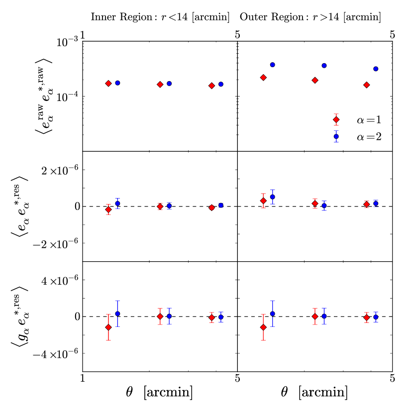
We tested the validity of our anisotropic PSF correction by measuring the auto-correlation function between stellar ellipticities and the cross-correlation function between stellar and galaxy ellipticities, before and after the correction. We found that $\langle e_{\alpha}^{*,\rm raw}e_{\alpha}^{*,\rm raw}\rangle$ and $\langle e_{\alpha}e_{\alpha}^{*,\rm raw}\rangle$ before the correction show large positive correlations ($\mathcal{O}(10^{-4})$), and that $\langle e_{\alpha}^{*,\rm res}e_{\alpha}^{*,\rm res}\rangle$ and $\langle e_{\alpha}^{\rm cor}e_{\alpha}^{*,\rm res}\rangle$ after the correction are consistent with null correlation in individual cluster fields. Note that $e_{\alpha}^{\rm cor}$ is the l.h.s. of Equation 1. In order to confirm how well the anisotropic PSF correction works at both the corners and centers, we divide the regions into the inner ($r<14^{\prime}$) and outer regions ($r>14^{\prime}$) of the fields of view with respect to the respective BCGs (Figure 1). Note that the BCGs are located close to the center of the field of view in all cases. The top-left and top-right panels show the cross-correlation function between stellar and galaxy ellipticities before the correction at the inner and outer regions, respectively. The raw distortions at the outer region is indeed larger than those at the inner region. The middle panel shows the resulting $\langle e_{\alpha}^{\rm cor}e_{\alpha}^{*,\rm res}\rangle$ after the correction, which are consistent with null correlation both at $r<14^{\prime}$ and $r>14^{\prime}$. The cross correlation between the residual stellar ellipticities and the reduced ellipticities for galaxies which are described in next paragraph is shown in the bottom panel. We again found null correlation at $r<14^{\prime}$ and $r>14^{\prime}$.

Figure 1: Top – The cross-correlation between raw ellipticities for stars an galaxies before the correction. The correlation at the outer region (right) is larger than that at the inner region (left). Middle – The cross-correlation between residual stellar ellipticities and corrected galaxy ellipticities. Bottom – The cross-correlation between residual stellar ellipticities and reduced ellipticities.

Next, we correct the isotropic smearing effect of galaxy shapes due to seeing and the Gaussian window function used for the shape measurements. The reduced ellipticity for each galaxy, $g_{\alpha}$, is defined by

$$g_{\alpha} = (P_{g}^{-1})_{\alpha\beta}e^{\prime}_{\beta},$$ (2)

where $(P_{g})_{\alpha\beta}$ is the pre-seeing shear polarizability tensor. The measurement of $(P_{g})_{\alpha\beta}$ is very noisy for individual faint galaxies because of its non-linearity (Bartelmann & Schneider 2001). The relationship between noise and biases in the measurement of faint galaxy shapes, using a variety of shape measurement algorithms, has been considered for both cosmic shear and cluster lensing studies (e.g. Hirata et al. 2004; Kacprzak et al. 2012; Melchior & Viola 2012; Refregier et al. 2012; Applegate et al. 2014; Hoekstra et al. 2015). The general feature of this relationship is that the bias in faint galaxy shape measurements typically increases as the size of galaxies decreases, i.e. as signal-to-noise ratio of galaxies decreases. In common with several authors (e.g. Umetsu et al. 2010; Oguri et al. 2012; Okura & Futamase 2012; Umetsu et al. 2015a) we have found that this dependence can be reduced significantly for KSB shape measurement methods if the galaxies upon which the isotropic PSF correction is based are limited to those detected at high signal-to-noise ratio (Okabe et al. 2013). We therefore calibrate the isotropic PSF correction, using galaxies detected at very high significance, i.e. a signal-to-noise ratio of $\nu>30$. This selection acts to suppress the measurement uncertainty of $(P_{g})_{\alpha\beta}$ that is caused by low signal-to-noise ratio in the objects used for the isotropic PSF correction in other studies. The polarizability tensor is first estimated by the scalar correction approximation $(P_{g})_{\alpha\beta}=\frac{1}{2}{\rm tr}[P_{g}]\delta_{\alpha\beta}$. We then compute the median of $(P_{g})_{\alpha\beta}$ in $r_{g}$, with an adaptive grid to assemble as uniformly as possible, where $r_{g}$ is the Gaussian smoothing radius used in the KSB method. We employ a size condition of $r_{h}>\bar{r}_{h}^{*}+\sigma(r_{h}^{*})$ and $r_{g}>\bar{r}_{g}^{*}+\sigma(r_{g}^{*})$ and a positive raw $P_{g}$. Here, $\bar{r}_{h}^{*}$ ($\sigma(r_{h}^{*})$) and $\bar{r}_{g}^{*}$ ($\sigma(r_{g}^{*})$) are the median (rms dispersion) of half-light radii and Gaussian smoothing radii for the stars used for the anisotropic PSF correction described above. Although galaxies and stars are well separated in $r_{h}$, we applied the cut in $r_{g}$ so as to exclude negative values of $P_{g}$ that are obtained for very small galaxies. We also checked the level of stellar contamination that galaxy catalogues, selected based on the size cuts described here, might suffer. We found that the level of contamination is below 1 per cent, mainly due to the fact that the number density of faint galaxies is an increasing function of apparent magnitude. The faint galaxies therefore out far out-number possible stellar contaminants.

We interpolate the polarizability tensor for individual galaxies with $\nu>10$ as a function of $r_{g}$ and the absolute value of the ellipticity, $|e|$. Here, we used $|e|$ instead of each component $e_{\alpha}$ because the isotropic PSF correction is performed by the half of the trace, $\frac{1}{2}{\rm tr}[P_{g}]\delta_{\alpha\beta}$ Then, in a major departure from Okabe et al. (2013), we applied a similar interpolation for the signal-to-noise ratio, $\nu$. An rms error of the ellipticity estimates, $\sigma_{g}$, is estimated from 50 neighbours in the magnitude-$r_{g}$ plane. We also experimented with smaller and larger numbers of neighbours and found that our results are unchanged.

2.5 Shape measurement tests

Figure 2: Top – Results of the shear measurement tests, showing the multiplicative bias, $m_{\alpha}$, for simulated observations ($0.7^{\prime\prime}$ seeing) of model galaxies (GLAFIC; Left) and realistic galaxies (SHERA; Right). The signal-to-noise ratio for the detection are $\nu>10$, matching the sample of galaxies that we select for our analysis. Red diamonds, and blue circles, green triangles and magenta squares denote $m_{1}$ and $m_{2}$ for GLAFIC and $m_{1}$ and $m_{2}$ for SHERA, respectively. The lower subpanels show the deviations from the input values. The dashed line shows $g_{\rm output}=g_{\rm input}$, and the solid line shows the result of the test described in the Section 2.5, in both upper and lower subpanels. Bottom – The shear measurement bias, $m_{\alpha}$, as a function of the magnitude and the Gaussian size using the imaging simulations of realistic galaxies (SHERA). Green triangles and magenta squares denote $m_{1}$ and $m_{2}$, respectively. The bias is not a strong function of galaxy size or magnitude.

We use two simulated datasets to test the reliability of our faint galaxy shape measurements, broadly following the approach introduced by the STEP programme (Heymans et al. 2006; Massey et al. 2007) with important modifications compared to STEP and the recent cluster weak-lensing literature. These modifications are designed to match our data, science goals, and our intention to use the weak-shear signal on scales of a few hundred kpc to constrain the shape of the matter density profile. The first modification is to test our ability to measure reduced shears upto $g\simeq 0.3$, as seen in the inner regions of clusters. The second modification is to produce simulated fits frames that match the angular size of the Suprime-Cam data; this allows us to include sufficient galaxies with $\nu>30$ that we can test our approach to the isotropic PSF correction. This is critical to validating that our shape measurement pipeline delivers accurate shapes at faint flux levels. We express the results of the tests outlined below following the STEP convention of:

$$g_{\alpha}-g_{\alpha}^{\rm input}=m_{\alpha}g_{\alpha}^{\rm input}+c_{\alpha}$$ (3)

where $g_{\alpha}$ and $g_{\alpha}^{\rm input}$ are the measured and input ellipticities, respectively; $m_{\alpha}$ is the multiplicative bias and $c_{\alpha}$ is a residual additive term.

Note that in both of the tests described below, we apply a constant shear to all of the simulated galaxies, and thus ignore higher order lensing effects that are present close to the Einstein radius (e.g. Okura, Umetsu & Futamase 2007). Higher order effects are negligible on the scale that we measure and fit the shear profile of clusters. The distribution of Einstein radii for a background redshift of $z=2$ for clusters from our sample that are known strong lenses is lognormal, peaking at $\theta_{\rm E}(z_{\rm S}=2)=14.5\,{\rm arcsec}$ (Richard et al. 2010). Rescaling this to the typical redshift of $z\simeq 0.8$ for the red background galaxies that we use in this analysis, we estimate $\theta_{\rm E}(z_{\rm S}=0.8)\simeq 12\,{\rm arcsec}$. Converting to physical projected distances, we therefore estimate an upper limit of $30h^{-1}{\rm kpc}$ on the typical Einstein radius at the median redshift of our cluster sample. Note that we regard this as an upper limit because half of our cluster sample have not been identified as strong lenses, and thus likely have smaller Einstein radii than the clusters discussed by Richard et al. (2010). For comparison, the innermost radius to which we typically fit the shear profile in Section 3.2 is $150h^{-1}{\rm kpc}$. Therefore, our shear analysis begins at clustercentric radii of $\mathrel{\hbox{\hbox to0.0pt{\hbox{\lower 4.0pt\hbox{$\sim$}}\hss}\hbox{$>$}}}5\,\theta_{\rm E}$, i.e. on scales where higher order lensing effects are negligible.

The first simulated dataset follows Okabe et al. (2013, note that these authors also tested their code upto $g\simeq 0.3$), and is based on simulated images, kindly provided by M. Oguri, that are generated with toy models using the software stuff (Bertin 2009). Each galaxy is characterized by bulge and disc components, with Sersic profiles indices of $n=4$ and $1$, respectively. Galaxy images are convolved with a PSF model based on the Moffat profile $\Sigma(R)\propto\left(1+(R/a)^{2}\right)^{-\beta}$, with seeing in the range $0.5\leq{\rm FWHM}\leq 1$arcsec and the Moffat profile with power slopes $3<\beta<12$, as described in Oguri et al. (2012). A number of fits frames matching the Suprime-Cam field of view were produced and analysed using the pipeline described in §2.4. We obtain a shear calibration bias of $m_{\alpha}\simeq-0.02$ and $c_{\alpha}\simeq 10^{-4}$ (Fig. 2).

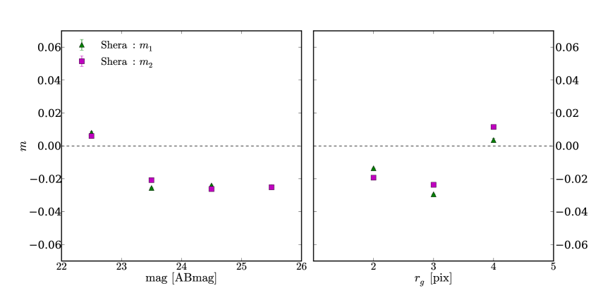
We extend Okabe et al.’s tests with a second simulated dataset, using the SHERA software (Mandelbaum et al. 2012) to generate simulated ground-based observations that match the properties of our observational data. The galaxies images included in these simulations are from the COSMOS Hubble Space Telescope observations, as described by Mandelbaum et al. in detail. We convolve the simulated data with a Moffat profile that matches our observational data: $\beta=4.6$ and ${\rm FWHM}=0.7\arcsec$. We generated both non-rotated and 90-degree rotated images to extract a shear estimate from a galaxy pair because the intrinsic ellipticity cancels out. The magnitude, size, and signal-to-noise ratio ($\nu$) distributions of the simulated galaxies match those of our Subaru data. We analyse these data using the same pipeline as above, obtaining again $m_{\alpha}\simeq-0.02$ and $c_{\alpha}\simeq 10^{-4}$ – i.e. consistent results from two methods of simulating the Subaru data (Fig. 2).

We also checked the magnitude and size dependence of the shear calibration using the SHERA-based simulations. The low level of shear bias detected above does not show a strong trend with size and magnitude, with $m_{\alpha}\simeq-0.02$ and $c_{\alpha}\simeq 10^{-4}$ (Fig. 2) down to apparent magnitudes of $i^{\prime}=26$. This result is achieved because of the high signal-to-noise threshold that we apply to galaxies used for the isotropic PSF correction described in §2.4.

In summary, our shape measurement bias is below our 4 per cent goal and does not depend on the size of galaxies. However we note that due to the finite number of galaxies used in our tests, in particular in the SHERA-based test (due to reliance on the COSMOS dataset), we cannot rule out the possibility that our shape measurement biases are different from those obtained here.

2.6 Photometry and redshift estimates

We will select faint background galaxies based on their location in the $(V-i^{\prime})/i^{\prime}$ colour magnitude plane in §2.7. We therefore analyse the data using SExtractor (Bertin & Arnouts 1996), adopting mag_auto as the total $i^{\prime}$-band magnitude of each object. $(V-i^{\prime})$ colours are measured in seeing matched frames, within an aperture of $1.5\times$ the FWHM of point sources in the poorer resolution of the two reduced frames for each cluster. Hereafter for convenience we often denote colour as $C=(V-i^{\prime})$.

Early-type cluster galaxies occupy a narrow well-defined relation in the colour-magnitude diagram – the so-called red-sequence. We fit a linear model of the form

$$(V-i^{\prime})_{\rm E/S0}=a\,i^{\prime}+b.$$ (4)

to galaxies at $i^{\prime}\leq 22$ in order to define the colour of the red sequence as a function of $i^{\prime}$-band magnitude for the purpose of selecting galaxies relative to the red sequence in §2.7.

Our overall strategy is to combine location in the colour-magnitude plane with redshift estimates and reduced shear measurements to identify a low contamination sample of background galaxies. The next step is therefore to estimate the redshift of each galaxy in the photometric catalogues. We base these estimates on the COSMOS UltraVISTA photometric redshift catalogue (McCracken et al. 2012; Ilbert et al. 2013) that is limited at $i^{\prime}<27.5$, and benefits from four deep near-infrared filters $Y$, $J$, $H$ and $K_{S}$. This filter coverage enables more robust photometric redshifts for galaxies at $z>1.3$ than earlier versions of the COSMOS catalogue, since the Balmer break is redshifted to the near-infrared for these galaxies. Furthermore, the COSMOS UltraVISTA photometric redshifts are tested against almost 35,000 new spectra with galaxies at $z>1.5$ (for more details see Ilbert et al. 2013). This catalogue provides currently the most reliable redshift distribution for a magnitude-limited galaxy sample that reaches $i^{\prime}\simeq 26$ with Suprime-Cam on Subaru. We emphasise that the COSMOS dataset includes observations through the same filters with the same camera mounted on the same telescope that we use in this study, thus matching LoCuSS and COSMOS photometry is straightforward.

The lensing kernel for the $i$-th galaxy in our photometric catalogues, $\beta_{i}\equiv{D_{ls,i}}/{D_{s,i}}$, is estimated by an ensemble average of the $N$ nearest neighbours in colour-magnitude space of the $i$-th galaxy in the COSMOS catalogue:

$$\beta_{i}=\langle{D_{ls}}/{D_{s}}\rangle_{\rm COSMOS}=\frac{1}{N}\sum_{j}^{N}{D_{ls,j}}({z_{s}})/{D_{s,j}}({z_{s}}).$$ (5)

Here, $D_{s}$ and $D_{ls}$ are the angular diameter distances from the observer to the sources and from the lens to the sources, respectively. The source redshift, $z_{s}$, is the median of the likelihood distribution for the photometric redshift of each COSMOS galaxy. We estimate the uncertainty on $\beta_{i}$ as the sum of the individual photometric errors and standard errors of the sample:

$$\sigma_{\beta}^{2}=\frac{1}{N}\sum_{j}^{N}\left[\sigma_{\beta^{\rm COSMOS},j}^{2}+\frac{1}{N-1}(\beta_{j}^{\rm COSMOS}-\beta)^{2}\right]$$ (6)

The typical uncertainties are $\sigma_{\beta}\simeq 13-28\%$. We adopt $N=100$, and check that our results are insensitive to whether we adopt $N=50$ or $N=200$ finding that the redshift estimates for individual galaxies are randomly changed by a few per cent. We include this small uncertainty in the redshift uncertainties that are incorporated in to the error bars on the cluster shear profiles in Section 3.2.

2.7 Selection of background galaxies

Contamination of background galaxy catalogues by unlensed member/foreground galaxies leads to a systematic underestimation of reduced shear signal. This is often referred to as a dilution effect, because the contaminants dilute the signal (Broadhurst et al. 2005; Umetsu et al. 2010; Okabe et al. 2010a, 2013). The dominant source of contaminant galaxies is faint cluster members, the number density of which increases towards the cluster core.

In Okabe et al. (2013) we quantified the contamination level as a function of the colour offset of faint galaxies from the red-sequence, defined by $\Delta C\equiv(V-i^{\prime})-(V-i^{\prime})_{\rm ES0}$, and concentrated on $\Delta C>0$, i.e. galaxies redder than the red sequence. We here briefly summarize the method. The mean tangential distortion strength is averaged over all galaxies satisfying a given colour cut, across all 50 clusters and all cluster-centric radii. The mean lensing signal increases strongly as a function of $\Delta C$ close to the red sequence, flattening to a shallower trend at larger colour offsets (see Fig. 1 of Okabe et al. 2013). We interpreted this behaviour with a two component model comprising contamination by cluster members and the redshift dependence of shear signal – i.e. redder galaxies are on average more distant and thus present a stronger lensing signal. The model includes a parameter that describes the fraction of the total population of galaxies that are contaminants from the cluster. Thus by fitting this model we were able to measure the contamination level and adopt a colour cut that gives a desired level of contamination without relying on any assumptions about the distribution of mass in the clusters, and about the run of number density of background galaxies with cluster-centric radius. We adopted $1\%$ contamination limit which is less than the statistical error of the average mass measurement for the sample of 50 clusters. However, this conservative approach yields a mean number density of background galaxies of just $\langle n_{\rm bkg}\rangle\sim 5.3\pm 1.9{\rm arcmin^{-2}}$, which makes it difficult to measure individual cluster masses without invoking assumptions about the shape of the cluster mass density profile.

Figure 3: Upper left: The mean lensing signal for all 50 clusters as a function of the colour offset $\Delta C$ in cluster-centric radial bins. The innermost bin has the largest shear signal (upper most set of points overlaid with brown curve), with progressively smaller shear signals seen at larger cluster-centric radii (lower sets of points overlaid with red through yellow, green and blue curves). All of the curves are flat at $\Delta C\mathrel{\hbox{\hbox to0.0pt{\hbox{\lower 4.0pt\hbox{$\sim$}}\hss}\hbox{$>$}}}0.5$ – i.e. at galaxy colours used for our analysis in Okabe et al. (2013). At smaller values of $\Delta C$ the curves relating to smaller cluster-centric radii steepen whilst those relating to larger cluster-centric radii are much flatter. The best-fit models are represented by the solid coloured curves. The legend states the typical weighted harmonic mean clustercentric radius of each radial bin. The dashed magenta curve denotes the location of the $1\%$ dilution level; the intersection between this curve and the solid curves indicates the colour cut required in each radial bin to achieve $1\%$ dilution. The vertical dotted green line is the $1\sigma$ width of the red sequence determined by the bright member galaxies. Lower left: The best-fit models of the dilution level of member galaxies as a function of the colour offset. The colours are the same as those in the upper left panel. The dilution level at innermost bin (brown) shows $\sim 40\%$ at $\Delta C=0$. The horizontal dashed line (magenta) is our requirement for the dilution level. Right: The colour-cut for background selection with $1\%$ dilution as a function of clustercentric radius. The colour cut is $\Delta C\sim 0.5$ at $r\sim 100~{}h^{-1}{\rm kpc}$ and $\Delta C=0$ beyond $\lower 2.15277pt\hbox{$\;\buildrel>\over{\sim}\;$}1.3~{}h^{-1}{\rm Mpc}$, respectively.

We develop a new method to select securely a larger sample of background galaxies than achieved by Okabe et al. (2013). In the new method, we average the mean tangential distortion strength over all galaxies satisfying each colour cut ($>\Delta C$) and all 50 clusters, in several radial bins. The stacked lensing strength in the $i$-th radial bin is estimated as:

$$\langle\Delta\Sigma_{+}\rangle(r_{i})=\frac{\sum_{n}g_{+,n}\Sigma_{{\rm cr},n}w_{n}}{\sum_{n}w_{n}},$$ (7)

where and $\Delta\Sigma_{+}$ is the dimensional reduced shear and the subscript $n$ denotes the $n$-th galaxy located in the annulus spanning $r_{1}<r_{i}<r_{2}$. Note that the reduced shear $\Delta\Sigma_{+}$ is different from the definition of, for example, Mandelbaum et al. (2006), because we define $\Delta\Sigma_{+}$ in terms of the reduced shear, $g$, and not in terms of shear, $\gamma$. The reduced tangential distortion component, $g_{+}$, with respect to the cluster center is defined by

$$g_{+} = -(g_{1}\cos 2\varphi+g_{2}\sin 2\varphi),$$ (8)

where $\varphi$ is the position angle between the first coordinate axis on the sky and the vector connecting the cluster center and the galaxy position. The reduced tangential shear is expressed by

$$g_{+}=\frac{\gamma_{+}}{1-\kappa},$$ (9)

where $\gamma_{+}$ is the tangential shear and $\kappa$ is the dimensionless surface mass density. The weighting functions are taken into account for both the statistical weights, $w_{n}$, and the critical projected mass density, $\Sigma_{{\rm cr},n}$, describing the lensing efficiency. The weighting $w_{n}$ (e.g. Hoekstra, Franx & Kuijken 2000; Hamana et al. 2003; Okabe et al. 2010a; Umetsu et al. 2010; Oguri et al. 2012) is used to down-weight galaxies whose shapes are less reliably measured, based on the uncertainty in the shape measurement, $\sigma_{g,n}$, given by

$$w_{n}=\frac{1}{\alpha^{2}+\sigma_{g,n}^{2}}\frac{1}{\Sigma_{{\rm cr},n}^{2}}.$$ (10)

We choose $\alpha=0.4$ throughout this paper. The critical projected mass density for individual clusters is defined by

$$\Sigma_{{\rm cr}}=\frac{c^{2}}{4\pi GD_{l}}\beta^{-1},$$ (11)

where $D_{l}$ is the angular diameter distance to a cluster and $\beta$ is the lensing depth (equation 5).

To clarify the relationship between $\Delta\Sigma_{+}$ and $g_{+}$ in the presence of contamination of background galaxy catalogues, we write an equation to describe the contamination effect, as follows:

$$\langle\Delta\Sigma_{+}\rangle = \frac{\sum_{n}(g_{+,n}\Sigma_{{\rm cr},n}w_{{\rm bkg},n}+0\times w_{{\rm non-bkg},n})}{\sum(w_{{\rm bkg},n}+w_{{\rm non-bkg},n})}$$ (12)

$$= \frac{\sum\Delta\Sigma_{+,n}w_{{\rm bkg},n}}{\sum(w_{{\rm bkg},n}+w_{{\rm non-bkg},n})},$$

where $\Delta\Sigma_{+}=g_{+}\Sigma_{cr}$ is the dimensional shear for each background galaxy and the subscripts “bkg” and“non-bkg” denote background galaxies and non-background galaxies, respectively. Since non-background galaxies are not lensed by the cluster, the second term in the numerator is zero. Therefore, contamination by non-background galaxies causes the observed lensing signal to be underestimated. The underestimation of the ensemble average is simply determined by the fraction of non-background galaxies (mainly member galaxies) to background galaxies. This is even clearer if, for the sake of illustration, one assumes that the galaxies have uniform weights, $w=1$, in which case Equation 12 can be rewritten as:

$$\langle\Delta\Sigma_{+}\rangle=\langle\Delta\Sigma_{+}\rangle_{\rm bkg}\frac{1}{1+n_{\rm non-bkg}/n_{\rm bkg}},$$ (13)

where $\langle\Delta\Sigma_{+}\rangle_{\rm bkg}$ is the average distortion strength using a pure sample of background galaxies. The correction factor, $(1+n_{\rm non-bkg}/n_{\rm bkg})$ is equivalent to the boost factor, under the assumption of a radially uniform distribution of background galaxies (e.g. Applegate et al. 2014; Hoekstra et al. 2015), that we discuss in Section 4.1.4. Equation 12 shows that the average lensing signal obtained from our formalism is simply underestimated by the fraction of non-background to background galaxies. Therefore also note that the non-linear term in the reduced shear $g_{+}=\gamma_{+}/(1-\kappa)\propto\Delta\Sigma_{+}$ does not impact on our estimated levels of contamination.

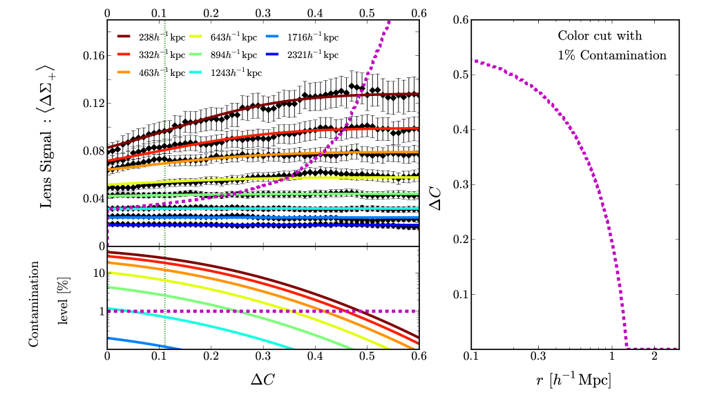
The stacked lensing signal is a decreasing function of clustercentric radius and an increasing function of $\Delta C$ for small clustercentric radii, reminiscent of Okabe et al.’s (2013) analysis of all clustercentric radii as a single bin (upper left panel of Fig. 3). However the increase in lensing signal at moderate values of $\Delta C$ becomes progressively less pronounced as one considers radial bins at larger clustercentric radii. This is qualitatively consistent with faint cluster galaxies being the dominant source of contamination, given that the number density of galaxies in clusters is a declining function of clustercentric radius.

To interpret quantitatively the mean lensing strength as a function of cluster-centric radius, we parameterise the galaxy distribution in terms of the projected clustercentric radius $r$ and the colour offset $\Delta C$, as follows:

$$n(r,\Delta C)=n_{b}(r)\left[1+Bf(\Delta C)n_{\rm m}(r)\right],$$ (14)

where $n_{b}(r)$ is the radial distribution of background galaxies. We do not assume any specific functions of $n_{b}$ because the background distribution is not constant, and may be depleted or boosted by a magnification bias (e.g. Broadhurst, Taylor & Peacock 1995; Umetsu et al. 2011, 2014; Coupon, Broadhurst & Umetsu 2013). The second term in the bracket denotes the member galaxy distribution; $B$ is the fraction, $f(\Delta C)$ is the colour distribution and $n_{\rm m}(r)$ is the radial distribution. The effective lensing strengths for red galaxies are obtained by integrating over the projected radius and the colour offset:

$$\langle\Delta\Sigma_{+,i}\rangle(r_{1}<r_{i}<r_{2},\Delta C<) = \frac{\int^{\infty}_{\Delta C}d(\Delta C)\int^{r_{2}}_{r_{1}}dr\Delta\Sigma_{+}n_{b}(r)r}{\int^{\infty}_{\Delta C}d(\Delta C)\int^{r_{2}}_{r_{1}}drn(r)r}$$ (15)

$$= \frac{A_{i}}{1+BF(\Delta C)N_{i}}.$$

Here, $A_{i}\equiv\Delta\Sigma_{+0,i}$ is the lensing signal estimated from the pure background galaxies and is thereby determined by the cluster mass distribution. The contamination levels in the colour and radial distributions are described by $F(\Delta C)=\int^{\infty}_{\Delta C}d(\Delta C)f(\Delta C)$ and $N_{i}=\int^{r_{2}}_{r_{1}}drn_{m}(r)r$, respectively. As in Okabe et al. (2013), we employ a Gaussian distribution centering at $\Delta C=0$ as the colour distribution of member galaxies,

$$F(\Delta C)=[1-{\rm erf}(\Delta C/\sqrt{2}\sigma)]/2,$$ (16)

where $\sigma$ is the width of colour distribution composed of the intrinsic scatter in the colour distribution and the photometric error. We assume that $\sigma$ is radius-independent. When we average equation (15) over all radial bins, the formulation in Okabe et al. (2013) is recovered:

$$\langle\langle\Delta\Sigma_{+}\rangle\rangle = \sum_{i}\langle\Delta\Sigma_{+,i}\rangle\simeq\tilde{A}\left[1-\tilde{B}F(\Delta C)\right].$$ (17)

In this paper, we simultaneously take into account the colour distribution and the radial distribution for member galaxies. We employ $n_{m}(r)=\exp(-r/r_{0})$ as the radial distribution of member galaxies (Applegate et al. 2014). Subsequently, fitting is performed to obtain the colour and radial distribution of member galaxies.

In summary, the fitting parameters are $A_{i}$, $B$, $\sigma$ and $r_{0}$. We stress that this method does not assume any specific mass models, which is important to interpret the results after defining the background sample. As shown in the upper left panel of Figure 3, the best-fit model (solid lines with different colours) well describes the data. The best-fit colour width, $\sigma=0.21$, is higher than the mean width expected from the intrinsic scatter determined by the cluster bright galaxies, which is consistent with Okabe et al. (2013). This large value of $\sigma$ is driven by the statistical scatter of the faint galaxies included in the calculation – i.e. the photometric uncertainties at $i^{\prime}\simeq 25$. We note that our method assumes that the colour distribution of galaxies redward of the red sequence is Gaussian; the large value of $\sigma$ therefore helps to ammeliorate any concerns that the wings of the actual distribution contain an excess of galaxies over the assumed Gaussian form. The characteristic radius of the member galaxy distribution is $r_{0}=258~{}\mathrel{h^{-1}{\rm kpc}}$. As expected based on the previous qualitative discussion, the highest level of contamination occurs at $\Delta C=0$ at the smallest clustercentric radii, with $F\simeq 0.4$ (Fig. 3), and the level of contamination declines significantly with increasing clustercentric radius. Contamination is negligible in the cluster outskirts. We conservatively adopt a limit of $1\%$ on contaminating fraction, and use this to define a radially dependent colour cut (right panel of Fig. 3). Note that at $r>1.3~{}\mathrel{h^{-1}{\rm Mpc}}$ the contamination level is so low that we adopt $\Delta C>0$ in this region. We achieve a number density of background galaxies of $n_{\rm bkg}\simeq 5-20~{}{\rm arcmin}^{-2}$ (Table 1), with a mean of $\langle n_{\rm bkg}\rangle\simeq 12.8~{}{\rm arcmin^{-2}}$ that is more than double that of Okabe et al. (2013).

We also use our mid- and far-infrared observations with Spitzer and Herschel as a sanity check on the possible impact of heavily dust-obscured galaxies on our red galaxy selection and on our COSMOS-based estimates of $\beta$ in the previous Section. Specifically, we consider whether dusty cluster members might leak into the red background galaxy samples and whether $\beta$ might be biased due to the presence of optically faint and heavily dust-obscured galaxies – i.e. Luminous Infrared Galaxies (LIRGs) and Ultra-Luminous Infrared Galaxies (ULIRGs). On the latter point, the COSMOS photometry extends to $8\mu{\rm m}$, whereas we have observed half of the cluster sample discussed in this article with Spitzer/MIPS at $24\mu{\rm m}$ (Haines et al. 2015) and with Herschel/PACS and SPIRE at $100-500\mu{\rm m}$ (Smith et al. 2010), albeit only to a depth corresponding to a bolometric infrared luminosity of $L_{\rm IR}\simeq 5\times 10^{10}L_{\odot}$ at $z\simeq 0.2$. The spectroscopic completeness of follow-up observations with Hectospec (Fabricant et al. 2005) is $96$ per cent for objects detected with Spitzer down to $0.5{\rm mJy}$ and and $\sim 80$ per cent down to $i=20$ (Mulroy et al. 2014; Haines et al. 2015). Clearly these data are not sensitive enough to obtain definitive estimates of the number and redshifts of dusty galaxies that satisfy our faint red optical background galaxy selection. However they provide a useful sanity check based on bright galaxies. We select galaxies from the catalogues discussed by Haines et al. (2015) at $i<20$ that have $(V-i)$ colours that would place them in our red background galaxy catalogues if they were faint enough. We find that $\sim 1$ per cent of these bright optically red galaxies are LIRGs, and $\sim 1$ per cent of the same bright optically red galaxies are cluster members, and there is no overlap between these two populations. We therefore conclude that the bright optically red galaxy population seen along lines of sight through our cluster sample appear to be consistent with (1) LIRGs and ULIRGs not being a significant population in our red background galaxy samples, and thus not being a concern in terms of the accuracy of $\beta$, and (2) our red background galaxy catalogues suffering just $1$ per cent contamination by cluster members.

3 Modelling and results

3.1 Model Fitting Methods

We describe how we compute the reduced tangential shear profile of each cluster and the model fitting procedure. We apply the methods described in this section to measure cluster masses in the next section.

We centre each cluster shear profile on the centroid of the optical emission from the cluster’s BCG, following numerous previous studies that have shown BCGs to be a reliable cluster centre for weak-lensing studies of massive galaxy clusters, including Okabe et al. (2010a, 2013), von der Linden et al. (2014), and Hoekstra et al. (2015). For example, we derived an upper limit of $32\,h^{-1}{\rm kpc}$ on the mean offset of BCGs from the underlying centre of the cluster mass distribution for the sample studied here, in Okabe et al. (2013). This upper limit is a factor of 5 smaller than the typical innermost radius of the shear profiles upon which our mass measurements are ultimately based in Section 3.2. Any bias caused by centring our shear profiles on the BCGs is therefore negligible.

The reduced shear in a given annulus centered on a given cluster is computed by azimuthally averaging the measured galaxy ellipticities, as defined by Equation 7. The mean redshift of the background galaxies is a function of cluster centric radius, due to our radially-dependent colour cut (Section 2.7). The formulation in equation 7 takes account of these differences by expressing the reduced shear in physics units.

We employ a maximum-likelihood method to model the shear profiles, and write the log-likelihood as follows:

$$-2\ln{\mathcal{L}} = \ln(\det(C_{ij}))+$$

$$\sum_{i,j}(\Delta\Sigma_{+,i}-f_{{\rm model}}(r_{i}))C_{ij}^{-1}(\Delta\Sigma_{+,j}-f_{{\rm model}}(r_{j})),$$

where the subscripts $i$ and $j$ are the $i-$ and $j-$th radial bins. Here, $f_{\rm model}$ is the reduced shear prediction for a specific mass model,

$$f_{{\rm model}}(r_{i})=\frac{\Delta\tilde{\Sigma}_{\rm model}(r_{i})}{1-K_{i}\Sigma_{\rm model}(r_{i}))},$$ (19)

where $\Sigma=\Sigma_{\rm cr}\kappa$ and $\Delta\tilde{\Sigma}=\Sigma_{\rm cr}\gamma$ are the convergence and the shear in physical units, respectively, and $\kappa$ and $\gamma$ are the dimensionless convergence and shear, respectively. The factor, $K_{i}$ for the $i$-th bin is given by:

$$K_{i}=\frac{\sum_{n}\Sigma_{\rm cr,n}^{-1}w_{n}}{\sum_{n}w_{n}}.$$ (20)

Note that $K_{i}$ is computed separately for each bin due to the radial dependence of the redshift of the background galaxies.

The covariance matrix, $C$, in equation 3.1 is given by:

$$C = C_{g}+C_{s}+C_{{\rm LSS}}.$$ (21)

Where the shape noise, $C_{g}$, in each radial bin is estimated as

$$C_{g,ij}=\frac{1}{2}\frac{\sum_{n}\sigma_{g,n}^{2}\Sigma_{\rm cr,n}^{2}w_{n}^{2}}{(\sum_{n}w_{n})^{2}}\delta_{ij},$$ (22)

where $\delta_{ij}$ is the Kronecker delta and the factor of $1/2$ accounts for the rms noise, $\sigma_{g,n}$, of two distortion components. The photometric redshift error matrix, $C_{s}$, is computed from:

$$C_{s,ij}=\tilde{C}_{s,ij}+\frac{\Delta\tilde{\Sigma}_{\rm model}^{2}\Sigma_{\rm model}^{2}\sigma_{K,i}^{2}}{(1-K_{i}\Sigma_{\rm model}(r_{i}))^{4}}\delta_{ij},$$ (23)

where the first term is given by

$$\tilde{C}_{s,ij}=\left[\frac{\sum_{n}(\Delta\Sigma_{+,n}-2\Delta\Sigma_{+})^{2}w_{n}^{2}(\sigma_{\Sigma,n}/\Sigma_{{\rm cr},n})^{2}}{(\sum_{n}w_{n})^{2}}\right]\delta_{ij}.$$

The second term of the equation (23) is the photometric redshift errors through an error of the conversion factor, $\sigma_{K}$, in the mass model (19). The covariance matrix of uncorrelated large-scale structure (LSS), $C_{\rm LSS}$, along the line-of-sight (Schneider et al. 1998) at an angular separation between $\theta_{i}=r_{i}/D_{l}$ and $\theta_{j}$ is given by

$$C_{{\rm LSS},ij}=\int\frac{ldl}{2\pi}P_{\kappa}(l)J_{2}(l\theta_{i})J_{2}(l\theta_{j}),$$ (24)

where $P_{\kappa}(l)$ is the weak-lensing power spectrum (e.g. Schneider et al. 1998; Hoekstra 2003), calculated by multipole $l$, the source redshift, and a given cosmology. We employ the redshift, ${\rm min}(z_{s,i},z_{s,j})$, and WMAP9 cosmology (Hinshaw et al. 2013). And, $J_{2}(l\theta_{i})$ is the Bessel function of the first kind and second order at the $i$-th annulus (Hoekstra 2003).

It is also important to compute the radius of each radial bin correctly, because systematic errors in the placement of the binned shear measurements on the radial axis can cause systematic errors in the mass measurement when a model is fitted. This is particularly important in practice, because the number density of background galaxies is neither uniform nor infinite. As described in detail in Appendix A, we found that the best radius at which to place the measurement of mean tangential shear in a radial bin is the weighted harmonic mean:

$$\langle r\rangle_{i}=\frac{\sum_{n}w_{n}}{\sum_{n}w_{n}\,r_{n}^{-1}},$$ (25)

where $w_{n}$ is given by Equation 10. We therefore compute bin radii in this way, in physics units, in the rest of our analysis.

Finally, before fitting models to the shear profiles (Section 3.2), we calculate the signal-to-noise ratio of the tangential shear profile as follows:

$$(S/N)^{2}=\sum_{ij}\Delta\Sigma_{+,i}(C_{g,ij}+\tilde{C}_{s,ij}+C_{{\rm LSS},ij})^{-1}\Delta\Sigma_{+,j}.$$ (26)

Each cluster is detected individually at signal-to-noise ratio of $3<S/N<11$ (Table 1).

3.2 Mass Measurements

To infer galaxy cluster masses from the shear profiles, we fit a model to the latter. For this purpose we adopt the universal mass density profile (Navarro, Frenk & White 1996, 1997b, hereafter NFW), that has had considerable success in describing dark matter halo profile spanning a wide mass range by numerical simulations based on the CDM model of structure formation. It has also been shown that the ensemble mass of a sample of clusters can be recovered to good precision from this approach, provided sufficient care is taken over the radial range over which this model is fitted to data (e.g. Becker & Kravtsov 2011; Bahé, McCarthy & King 2012).

The NFW profile is expressed in the form:

$$\rho_{\rm NFW}(r)=\frac{\rho_{s}}{(r/r_{s})(1+r/r_{s})^{2}},$$ (27)

where $\rho_{s}$ is the central density parameter and $r_{s}$ is the scale radius. The three-dimensional spherical mass, $M_{\Delta}$, enclosed by the radius, $r_{\Delta}$, inside of which the mean density is $\Delta$ times the critical mass density, $\rho_{\rm cr}(z)$, at the redshift, $z$, is given by

$$M_{\rm NFW}(<r_{\Delta})=\frac{4\pi\rho_{s}r_{\Delta}^{3}}{c_{\Delta}^{3}}\left[\ln(1+c_{\Delta})-\frac{c_{\Delta}}{1+c_{\Delta}}\right].$$ (28)

The NFW profile is fully specified by two parameters: $M_{\Delta}$ and the halo concentration $c_{\Delta}=r_{\Delta}/r_{s}$. We fit this model to the shear profile of each cluster, taking full account of errors of shape measurements, photometric redshifts and the uncorrelated LSS (Section 3.1). For a given $M_{\Delta}$ and $c_{\Delta}$ we predict the observed shear signal following the formalism described by Wright & Brainerd (2000).

Measurements of $M_{\Delta}$ are mainly sensitive to the lensing signal around the overdensity radii $r_{\Delta}$ (Okabe et al. 2010a). However the concentration parameter, $c_{\Delta}$, is more strongly affected by the lensing signal in the cluster central regions, i.e. cluster centric radii of hundreds of kpc. Our careful selection of background galaxies ensures that contamination of our background galaxy samples is negligible across the full radial range of our shear profiles. However the very stringent colour cut employed in the central regions, $\Delta\,C>0.52$, and the relatively small solid angle subtended by these innermost bins, render them the noisiest of the entire radial range. To guard against obtaining results on concentration that suffer biases due to the noisy inner profiles, we choose a binning scheme for each cluster via the following procedure. We fit the NFW model to a suite of measured shear profiles that span inner radii in the range $r_{\rm in}=50-300~{}h^{-1}{\rm kpc}$, outer radii in the range $r_{\rm out}=2000-3000~{}h^{-1}{\rm kpc}$, and number of bins in the range $N_{\rm bin}=4-8$. We then compute the mean of the suite of $M_{\Delta}$ values obtained from these fits, and adopt the binning scheme that yields the value of $M_{\Delta}$ closest to that mean. Note that we allow the virial concentration parameter to be in the range $0<c_{\rm vir}<30$ in the fits. Also, we restrict the radial range of the shear profile fits for A1758N to $r_{\rm out}<2100h^{-1}{\rm kpc}$ to avoid contamination of lensing signal by its neighbour A1758S. Note that we test the procedure described above using mock observations of simulated and toy model clusters, and confirm that it returns masses and concentrations with negligible bias (Section 4.1.1).

Figure 4: Radial profiles of the tangential shear component (top panel), $\Delta\Sigma_{+}$, and the product of the $45$ degree rotated component, $\Delta\Sigma_{\times}$, and clustercentric radius, $r$

(bottom panel), , for ABELL 2390 (left) and ABELL 0901 (right), respectively.

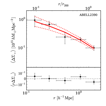
Figure 4 shows the tangential distortion profiles as a function of the projected cluster-centric radius for two example clusters, ABELL 2390 and ABELL 0901. The former is among the most massive in the sample and the latter among the least massive. The tangential shear clearly decreases from the cluster centre to the outskirts, with the less massive cluster, ABELL 0901, presenting an overall shear signal of approximately half that of the more massive cluster, ABELL 2390. Note that the $45$ degree rotated component times the clustercentric radius $r$, $r\Delta\Sigma_{\times}$, is consistent with zero – i.e. this simple test of residual systematics is consistent with zero.

Table 2 lists $M_{\Delta}$ from our weak-lensing analysis, defined as $M_{\Delta}=\Delta\mathrel{\rho_{\rm crit}}(z)4\pi r_{\Delta}^{3}/3$ where $\mathrel{\rho_{\rm crit}}(z)$ is the critical density of the universe at the respective cluster redshifts, and $\Delta=\Delta_{\rm vir}$, $200$, $500$, $1000$, and $2500$. We also list $M_{\Delta}$ defined as $M_{\Delta}=\Delta\rho_{\rm m}(z)4\pi r_{\Delta}^{3}/3$, where $\rho_{\rm m}(z)=\mathrel{\rho_{\rm crit}}(z)\Omega_{\rm M}(z)$ is the mean matter density of the universe, and $\Delta=180$ and $200$. We denote these latter two masses as $M_{\rm 180m}$ and $M_{\rm 200m}$ respectively.

Table 2: Mass measures for individual clusters on $\langle M_{\Delta}\rangle_{\rm cog}$

Name	$M_{\rm vir}$	$M_{200}$	$M_{500}$	$M_{1000}$	$M_{2500}$	$M_{180{\rm m}}$	$M_{200{\rm m}}$
	$10^{14}\mathrel{h^{-1}M_{\odot}}$	$10^{14}\mathrel{h^{-1}M_{\odot}}$	$10^{14}\mathrel{h^{-1}M_{\odot}}$	$10^{14}\mathrel{h^{-1}M_{\odot}}$	$10^{14}\mathrel{h^{-1}M_{\odot}}$	$10^{14}\mathrel{h^{-1}M_{\odot}}$	$10^{14}\mathrel{h^{-1}M_{\odot}}$
ABELL2697	$10.37_{-2.23}^{+3.26}$	$8.03_{-1.48}^{+1.88}$	$4.62_{-0.84}^{+0.84}$	$2.72_{-0.80}^{+0.73}$	$1.12_{-0.53}^{+0.61}$	$12.29_{-2.92}^{+4.65}$	$11.76_{-2.73}^{+4.25}$
ABELL0068	$7.78_{-1.47}^{+1.76}$	$6.65_{-1.16}^{+1.35}$	$4.78_{-0.71}^{+0.78}$	$3.51_{-0.48}^{+0.50}$	$2.12_{-0.36}^{+0.34}$	$8.64_{-1.71}^{+2.09}$	$8.39_{-1.64}^{+2.00}$
ABELL2813	$9.47_{-2.02}^{+2.53}$	$8.17_{-1.61}^{+1.91}$	$5.90_{-0.97}^{+1.06}$	$4.37_{-0.70}^{+0.72}$	$2.66_{-0.65}^{+0.58}$	$10.43_{-2.35}^{+3.02}$	$10.14_{-2.25}^{+2.87}$
ABELL0115	$9.49_{-2.94}^{+4.56}$	$7.04_{-1.97}^{+2.66}$	$3.77_{-1.04}^{+1.14}$	$2.07_{-0.77}^{+0.77}$	$0.75_{-0.40}^{+0.51}$	$11.60_{-3.84}^{+6.60}$	$11.06_{-3.60}^{+6.04}$
ABELL0141	$5.67_{-1.23}^{+1.45}$	$4.71_{-0.95}^{+1.08}$	$3.19_{-0.60}^{+0.65}$	$2.22_{-0.48}^{+0.48}$	$1.21_{-0.38}^{+0.38}$	$6.42_{-1.46}^{+1.78}$	$6.22_{-1.39}^{+1.69}$
ZwCl0104.4+0048	$2.71_{-1.09}^{+1.66}$	$2.24_{-0.81}^{+1.01}$	$1.47_{-0.74}^{+0.56}$	$0.99_{-0.70}^{+0.48}$	$0.51_{-0.53}^{+0.46}$	$3.08_{-1.32}^{+2.46}$	$2.98_{-1.26}^{+2.21}$
ABELL0209	$15.42_{-2.54}^{+3.14}$	$12.75_{-1.91}^{+2.27}$	$8.64_{-1.05}^{+1.15}$	$5.99_{-0.65}^{+0.68}$	$3.26_{-0.49}^{+0.46}$	$17.57_{-3.07}^{+3.90}$	$17.01_{-2.93}^{+3.70}$
ABELL0267	$7.28_{-1.33}^{+1.58}$	$5.97_{-1.08}^{+1.16}$	$3.92_{-0.59}^{+0.64}$	$2.63_{-0.42}^{+0.43}$	$1.35_{-0.31}^{+0.30}$	$8.33_{-1.60}^{+1.95}$	$8.04_{-1.53}^{+1.85}$
ABELL0291	$7.47_{-1.92}^{+2.68}$	$5.63_{-1.28}^{+1.61}$	$3.12_{-0.67}^{+0.71}$	$1.77_{-0.52}^{+0.50}$	$0.68_{-0.30}^{+0.35}$	$9.05_{-2.51}^{+3.80}$	$8.64_{-2.35}^{+3.50}$
ABELL0383	$6.27_{-1.42}^{+1.83}$	$5.23_{-1.07}^{+1.30}$	$3.64_{-0.60}^{+0.65}$	$2.59_{-0.37}^{+0.39}$	$1.48_{-0.33}^{+0.29}$	$7.11_{-1.71}^{+2.30}$	$6.90_{-1.64}^{+2.18}$
ABELL0521	$6.76_{-1.36}^{+1.58}$	$5.61_{-1.05}^{+1.18}$	$3.77_{-0.65}^{+0.69}$	$2.59_{-0.51}^{+0.51}$	$1.39_{-0.40}^{+0.40}$	$7.65_{-1.62}^{+1.93}$	$7.40_{-1.54}^{+1.83}$
ABELL0586	$7.69_{-2.05}^{+2.99}$	$6.65_{-1.61}^{+2.15}$	$5.04_{-0.98}^{+1.12}$	$3.92_{-0.64}^{+0.69}$	$2.60_{-0.68}^{+0.53}$	$8.53_{-2.41}^{+3.72}$	$8.32_{-2.32}^{+3.54}$
ABELL0611	$10.89_{-2.12}^{+2.46}$	$9.23_{-1.71}^{+1.92}$	$6.37_{-1.09}^{+1.17}$	$4.51_{-0.80}^{+0.82}$	$2.54_{-0.60}^{+0.58}$	$12.14_{-2.45}^{+2.91}$	$11.77_{-2.35}^{+2.77}$
ABELL0697	$12.62_{-3.14}^{+4.87}$	$9.74_{-2.13}^{+2.90}$	$5.39_{-1.00}^{+1.08}$	$3.05_{-0.81}^{+0.76}$	$1.17_{-0.51}^{+0.56}$	$14.91_{-4.01}^{+6.72}$	$14.22_{-3.73}^{+6.14}$
ZwCl0857.9+2107	$3.12_{-1.20}^{+1.58}$	$2.45_{-0.91}^{+1.09}$	$1.45_{-0.75}^{+0.69}$	$0.88_{-0.59}^{+0.57}$	$0.37_{-0.42}^{+0.45}$	$3.67_{-1.47}^{+2.14}$	$3.52_{-1.39}^{+1.97}$
ABELL0750	$7.66_{-2.34}^{+3.98}$	$6.30_{-1.74}^{+2.71}$	$4.31_{-0.95}^{+1.20}$	$3.02_{-0.54}^{+0.60}$	$1.67_{-0.46}^{+0.39}$	$8.78_{-2.85}^{+5.14}$	$8.51_{-2.72}^{+4.86}$
ABELL0773	$11.11_{-1.45}^{+1.67}$	$9.56_{-1.14}^{+1.28}$	$7.05_{-0.70}^{+0.75}$	$5.33_{-0.48}^{+0.50}$	$3.37_{-0.39}^{+0.37}$	$12.31_{-1.70}^{+2.00}$	$12.00_{-1.63}^{+1.91}$
ABELL0781	$8.17_{-2.25}^{+3.01}$	$6.57_{-1.65}^{+1.97}$	$3.97_{-1.19}^{+1.11}$	$2.46_{-1.10}^{+0.93}$	$1.09_{-0.69}^{+0.77}$	$9.40_{-2.77}^{+4.06}$	$9.02_{-2.60}^{+3.72}$
ZwCl0949.6+5207	$5.02_{-1.34}^{+1.72}$	$4.44_{-1.10}^{+1.32}$	$3.48_{-0.73}^{+0.79}$	$2.79_{-0.53}^{+0.56}$	$1.96_{-0.53}^{+0.44}$	$5.47_{-1.54}^{+2.06}$	$5.35_{-1.49}^{+1.97}$
ABELL0901	$3.11_{-0.97}^{+1.26}$	$2.65_{-0.77}^{+0.95}$	$1.95_{-0.50}^{+0.57}$	$1.48_{-0.36}^{+0.39}$	$0.93_{-0.31}^{+0.29}$	$3.48_{-1.14}^{+1.54}$	$3.39_{-1.10}^{+1.47}$
ABELL0907	$18.97_{-4.66}^{+8.04}$	$14.28_{-2.99}^{+4.59}$	$8.07_{-1.17}^{+1.37}$	$4.66_{-0.78}^{+0.75}$	$1.85_{-0.61}^{+0.62}$	$23.03_{-6.19}^{+11.51}$	$22.06_{-5.83}^{+10.61}$
ABELL0963	$8.59_{-1.56}^{+1.87}$	$7.13_{-1.20}^{+1.38}$	$4.87_{-0.72}^{+0.78}$	$3.41_{-0.53}^{+0.54}$	$1.88_{-0.42}^{+0.41}$	$9.77_{-1.88}^{+2.31}$	$9.46_{-1.79}^{+2.20}$
ZwCl1021.0+0426	$6.11_{-1.22}^{+1.43}$	$5.24_{-0.96}^{+1.09}$	$3.73_{-0.57}^{+0.61}$	$2.72_{-0.41}^{+0.42}$	$1.61_{-0.37}^{+0.34}$	$6.76_{-1.42}^{+1.72}$	$6.56_{-1.36}^{+1.63}$
ABELL1423	$5.05_{-1.26}^{+1.67}$	$4.30_{-0.97}^{+1.19}$	$3.11_{-0.57}^{+0.62}$	$2.30_{-0.43}^{+0.43}$	$1.41_{-0.45}^{+0.37}$	$5.64_{-1.49}^{+2.09}$	$5.48_{-1.43}^{+1.98}$
ABELL1451	$10.27_{-1.42}^{+1.64}$	$8.54_{-1.08}^{+1.22}$	$5.88_{-0.63}^{+0.67}$	$4.15_{-0.42}^{+0.43}$	$2.32_{-0.31}^{+0.30}$	$11.67_{-1.71}^{+2.01}$	$11.31_{-1.63}^{+1.92}$
RXCJ1212.3-1816	$2.44_{-1.08}^{+1.48}$	$2.12_{-0.91}^{+1.17}$	$1.55_{-0.63}^{+0.75}$	$1.17_{-0.49}^{+0.54}$	$0.73_{-0.40}^{+0.37}$	$2.69_{-1.22}^{+1.74}$	$2.62_{-1.18}^{+1.67}$
ZwCl1231.4+1007	$7.20_{-2.09}^{+2.91}$	$5.58_{-1.49}^{+1.82}$	$3.23_{-1.03}^{+1.01}$	$1.91_{-0.86}^{+0.83}$	$0.79_{-0.49}^{+0.66}$	$8.53_{-2.65}^{+4.09}$	$8.17_{-2.49}^{+3.75}$
ABELL1682	$10.35_{-1.57}^{+1.85}$	$8.66_{-1.21}^{+1.38}$	$5.97_{-0.69}^{+0.75}$	$4.21_{-0.44}^{+0.46}$	$2.36_{-0.33}^{+0.31}$	$11.69_{-1.87}^{+2.25}$	$11.33_{-1.79}^{+2.14}$
ABELL1689	$12.34_{-1.78}^{+2.07}$	$10.98_{-1.46}^{+1.66}$	$8.80_{-0.98}^{+1.07}$	$7.22_{-0.69}^{+0.72}$	$5.28_{-0.47}^{+0.47}$	$13.41_{-2.04}^{+2.40}$	$13.15_{-1.97}^{+2.32}$
ABELL1758N	$6.76_{-1.64}^{+2.08}$	$5.88_{-1.32}^{+1.53}$	$4.35_{-0.97}^{+0.98}$	$3.29_{-1.02}^{+0.87}$	$2.09_{-1.02}^{+0.90}$	$7.42_{-1.91}^{+2.57}$	$7.22_{-1.83}^{+2.42}$
ABELL1763	$20.69_{-3.71}^{+4.97}$	$16.92_{-2.70}^{+3.42}$	$11.06_{-1.36}^{+1.51}$	$7.40_{-0.84}^{+0.86}$	$3.77_{-0.73}^{+0.68}$	$23.71_{-4.55}^{+6.31}$	$22.89_{-4.32}^{+5.94}$
ABELL1835	$11.50_{-2.05}^{+2.43}$	$10.09_{-1.63}^{+1.88}$	$7.68_{-1.01}^{+1.09}$	$5.99_{-0.72}^{+0.74}$	$4.00_{-0.68}^{+0.64}$	$12.57_{-2.38}^{+2.88}$	$12.27_{-2.28}^{+2.75}$
ABELL1914	$11.04_{-2.22}^{+2.87}$	$8.73_{-1.59}^{+1.92}$	$5.48_{-0.87}^{+0.94}$	$3.51_{-0.63}^{+0.64}$	$1.66_{-0.47}^{+0.47}$	$12.98_{-2.79}^{+3.78}$	$12.51_{-2.65}^{+3.55}$
ZwCl1454.8+2233	$5.61_{-2.29}^{+4.55}$	$4.42_{-1.62}^{+2.47}$	$2.62_{-1.01}^{+1.03}$	$1.58_{-0.91}^{+0.78}$	$0.68_{-0.66}^{+0.67}$	$6.54_{-2.85}^{+6.80}$	$6.28_{-2.69}^{+6.10}$
ABELL2009	$10.29_{-3.15}^{+5.75}$	$7.78_{-2.03}^{+3.19}$	$4.47_{-0.87}^{+1.02}$	$2.63_{-0.69}^{+0.64}$	$1.07_{-0.49}^{+0.56}$	$12.49_{-4.18}^{+8.40}$	$11.97_{-3.93}^{+7.74}$
ZwCl1459.4+4240	$3.51_{-1.01}^{+1.20}$	$3.17_{-0.87}^{+1.01}$	$2.56_{-0.64}^{+0.71}$	$2.11_{-0.50}^{+0.53}$	$1.56_{-0.38}^{+0.38}$	$3.75_{-1.11}^{+1.34}$	$3.68_{-1.08}^{+1.30}$
RXCJ1504.1-0248	$6.10_{-1.45}^{+1.73}$	$5.53_{-1.25}^{+1.46}$	$4.58_{-0.93}^{+1.04}$	$3.87_{-0.71}^{+0.77}$	$2.99_{-0.49}^{+0.51}$	$6.54_{-1.56}^{+1.94}$	$6.42_{-1.55}^{+1.89}$
ABELL2111	$5.78_{-1.92}^{+4.87}$	$4.93_{-1.48}^{+2.68}$	$3.56_{-0.85}^{+0.97}$	$2.63_{-1.09}^{+0.67}$	$1.60_{-1.14}^{+0.64}$	$6.43_{-2.28}^{+6.93}$	$6.26_{-2.18}^{+6.35}$
ABELL2204	$11.32_{-2.36}^{+3.07}$	$9.56_{-1.83}^{+2.29}$	$6.95_{-1.11}^{+1.27}$	$5.17_{-0.70}^{+0.76}$	$3.18_{-0.46}^{+0.45}$	$12.77_{-2.81}^{+3.75}$	$12.43_{-2.71}^{+3.59}$
ABELL2219	$13.38_{-2.60}^{+3.55}$	$10.40_{-1.75}^{+2.15}$	$6.06_{-0.91}^{+0.94}$	$3.60_{-0.81}^{+0.74}$	$1.50_{-0.57}^{+0.60}$	$15.83_{-3.38}^{+4.92}$	$15.17_{-3.16}^{+4.53}$
RXJ1720.1+2638	$6.45_{-1.94}^{+2.85}$	$5.23_{-1.45}^{+1.96}$	$3.46_{-0.82}^{+0.97}$	$2.34_{-0.53}^{+0.58}$	$1.22_{-0.40}^{+0.38}$	$7.48_{-2.37}^{+3.66}$	$7.23_{-2.26}^{+3.46}$
ABELL2261	$14.85_{-2.55}^{+3.29}$	$11.93_{-1.80}^{+2.18}$	$7.52_{-0.84}^{+0.91}$	$4.85_{-0.56}^{+0.55}$	$2.32_{-0.50}^{+0.47}$	$17.20_{-3.19}^{+4.28}$	$16.56_{-3.01}^{+4.01}$
RXCJ2102.1-2431	$4.16_{-1.06}^{+1.29}$	$3.55_{-0.85}^{+0.99}$	$2.60_{-0.56}^{+0.61}$	$1.95_{-0.40}^{+0.43}$	$1.21_{-0.32}^{+0.30}$	$4.65_{-1.23}^{+1.54}$	$4.53_{-1.19}^{+1.48}$
RXJ2129.6+0005	$6.34_{-2.00}^{+2.99}$	$4.69_{-1.29}^{+1.63}$	$2.42_{-0.85}^{+0.79}$	$1.28_{-0.65}^{+0.64}$	$0.44_{-0.30}^{+0.45}$	$7.74_{-2.67}^{+4.60}$	$7.35_{-2.48}^{+4.11}$
ABELL2390	$12.61_{-2.14}^{+2.53}$	$10.60_{-1.67}^{+1.91}$	$7.37_{-0.99}^{+1.06}$	$5.25_{-0.64}^{+0.67}$	$2.99_{-0.47}^{+0.44}$	$14.18_{-2.52}^{+3.05}$	$13.75_{-2.42}^{+2.91}$
ABELL2485	$6.90_{-1.51}^{+1.91}$	$5.72_{-1.13}^{+1.33}$	$3.83_{-0.64}^{+0.69}$	$2.63_{-0.54}^{+0.50}$	$1.40_{-0.48}^{+0.45}$	$7.82_{-1.83}^{+2.42}$	$7.56_{-1.74}^{+2.27}$
ABELL2537	$8.55_{-2.27}^{+2.90}$	$7.65_{-1.90}^{+2.31}$	$6.00_{-1.27}^{+1.42}$	$4.82_{-0.94}^{+1.00}$	$3.40_{-0.88}^{+0.78}$	$9.21_{-2.55}^{+3.37}$	$9.01_{-2.47}^{+3.22}$
ABELL2552	$9.14_{-2.74}^{+4.33}$	$7.61_{-2.08}^{+2.88}$	$5.01_{-1.18}^{+1.32}$	$3.38_{-1.06}^{+0.94}$	$1.74_{-0.90}^{+0.83}$	$10.30_{-3.27}^{+5.61}$	$9.94_{-3.11}^{+5.20}$
ABELL2631	$9.26_{-2.51}^{+3.73}$	$7.13_{-1.66}^{+2.07}$	$3.93_{-1.25}^{+1.10}$	$2.22_{-1.08}^{+1.05}$	$0.84_{-0.56}^{+0.89}$	$10.96_{-3.30}^{+5.57}$	$10.45_{-3.06}^{+4.98}$
ABELL2645	$5.00_{-1.27}^{+1.53}$	$4.16_{-0.99}^{+1.15}$	$2.81_{-0.64}^{+0.69}$	$1.95_{-0.52}^{+0.52}$	$1.05_{-0.40}^{+0.41}$	$5.65_{-1.49}^{+1.86}$	$5.46_{-1.43}^{+1.76}$

3.3 Mass-Concentration Relation

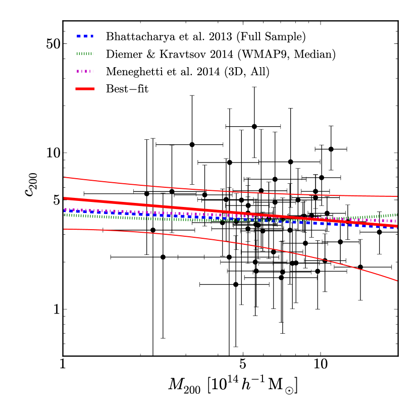
Numerical simulations (e.g. Bullock et al. 2001; Duffy et al. 2008; Bhattacharya et al. 2013; Diemer & Kravtsov 2014; Meneghetti et al. 2014; Ludlow et al. 2014) predict that the halo concentration $c_{\Delta}$ and the mass $M_{\Delta}$ for the NFW mass model is weakly anti-correlated. Such a correlation is naturally explained by the hierarchical structure formation, that is, less massive halos first form and more massive halos form through mass accretion and mergers of smaller objects. The characteristic central density of more massive halos is lower as reflected by the critical mass density of the universe at the redshift of collapse. Measurements of cluster mass and concentration therefore provide us with a unique opportunity to test structure formation.

Our cluster sample is selected purely on X-ray luminosities without imposing any requirement on the physical properties of the clusters. In particular, we do not select on the dynamical state of clusters as inferred from their X-ray morphology. We are therefore able to investigate the correlation between mass and concentration for a large sample of clusters that is unbiased beyond that which is inherent to an X-ray selection. A typical cluster in our sample has a concentration of $c_{200}\simeq 4$ (Figure 5), with central values of $c_{200}$ in the range $c_{200}\sim 2-20$. We quantify the mass-concentration correlation with the following function:

$$c_{\Delta}(M_{\Delta})=c_{0}\left(\frac{M_{\Delta}}{10^{14}\mathrel{h^{-1}M_{\odot}}}\right)^{b},$$ (29)

where $c_{0}$ and $b$ are the normalization of the concentration parameter at $M_{\Delta}=10^{14}\mathrel{h^{-1}M_{\odot}}$ and the slope, respectively. This form is motivated by the studies of the numerical simulations (e.g. Bullock et al. 2001). Note that we ignore redshift evolution in this model because the redshift range of our sample is narrow. When we fit this model, we take account of the correlation between the errors on concentration and mass by calculating the error covariance matrix, and include the intrinsic scatter of the lensing-based concentration parameter, $\sigma_{\rm int}$. The log-likelihood is given by:

$$-2\ln{\mathcal{L}} = \sum_{i}\ln\left(\sigma_{\ln c,i}^{2}+b^{2}\sigma_{\ln M,i}^{2}-2b\sigma_{\ln c,\ln M,i}+\sigma_{\rm int}^{2}\right)$$

$$+\sum_{i}\frac{(\ln(c_{i})-(a+b\ln(M_{i})))^{2}}{\sigma_{\ln c,i}^{2}+b^{2}\sigma_{\ln M,i}^{2}-2b\sigma_{\ln c,\ln M,i}+\sigma_{\rm int}^{2}},$$

where $a=\log(c_{0})$ and $\sigma_{\ln c}$ and $\sigma_{\ln M}$ are the fractional errors of the concentration and the mass, $\sigma_{\ln c,\ln M}$ is the error correlation, and $\sigma_{\rm int}$ is the intrinsic scatter in $\ln c$. We perform the fitting at overdensities of $\Delta=180{\rm m},200{\rm m},{\rm vir}$, and $200$. The normalisation of our best-fit mass-concentration relation is in excellent agreement with the results of recent numerical simulations at $z_{l}=0.23$ (Table 3; Figure 5; Bhattacharya et al. 2013; Diemer & Kravtsov 2014; Meneghetti et al. 2014). As an aside, we note that these three recent independent theoretical studies agree both with each other and with our observational results, whilst older simulations showed considerable variation between their respective mass-concentration relations and a lower overall normalization (e.g. Duffy et al. 2008; Stanek et al. 2010). The best-fit slopes agree with the weak-mass dependence of the concentration, $b\simeq-0.1$, seen in simulations (Table 3), although the uncertainties are too large to rule out positive values of $b$. Adding less massive clusters and increasing the number density of background galaxies will allow improved constraints in future studies.

Table 3: Best-fit parameters for the mass concentration relation.

$\Delta$	$c_{0}$	$b$	$\sigma_{\rm int}$
$180{\rm m}$	$9.24^{+3.99}_{-2.50}$	$-0.20_{-0.15}^{+0.13}$	$<0.17$
$200{\rm m}$	$8.74^{+3.75}_{-2.49}$	$-0.19_{-0.15}^{+0.14}$	$<0.17$
Virial	$7.26^{+3.18}_{-2.07}$	$-0.17_{-0.16}^{+0.15}$	$<0.18$
$200$	$5.12^{+2.08}_{-1.44}$	$-0.14_{-0.16}^{+0.16}$	$<0.20$

Figure 5: The observed distribution of the concentration parameters $c_{\rm 200}$ as a function of the cluster masses $M_{\rm 200}$ for 50 clusters. The errors denote 68% confidence intervals. The thick and thin lines (red) are the best-fit function and the errors, respectively. The dashed blue, dotted green and dotted-dashed magenta lines are the mean mass-concentration relation from recent numerical simulations of Bhattacharya et al. (2013), Diemer & Kravtsov (2014) and Meneghetti et al. (2014) at $z_{l}=0.23$, respectively.

3.4 Stacked Lensing Analysis

Figure 6: Stacked tangential shear profile for 50 clusters. The errors are composed of $(C_{g,ii}+\tilde{C}_{s,ii}+C_{{\rm LSS},ii})^{1/2}$. Thick solid red and dashed green lines are the total mass and the NFW model, respectively. The dotted blue and dashed-dotted magenta lines are the two-halo term and point source multiplied by 10, respectively.

Stacked lensing analysis is a powerful technique for measuring the average density profile of a sample of clusters. Stacking the shear signal from a sample of clusters averages over the distribution of internal structures and halo triaxiality, and thus overcomes the structural biases suffered by some individual cluster mass measurements (e.g. Mandelbaum et al. 2006; Johnston et al. 2007; Okabe et al. 2010a, 2013; Umetsu et al. 2011, 2014, 2015b; Oguri et al. 2012; Leauthaud et al. 2012; Miyatake et al. 2013; Niikura et al. 2015).

We compute the average lensing signal in physical length unit centered on the respective BCGs. Note that our redshift range is narrow, and therefore the results described below are unchanged if we instead use comoving length units. Moreover, we have previously tested that adopting physical length units, and not scaling length to an overdensity radius, yields an unbiased measurement of the stacked shear profile of our sample (Okabe et al. 2013). The innermost radius of the stacked shear profile is that at which the innermost bin of the stacked profile contains a minimum of one background galaxy from each cluster. The outermost radius of the stacked profile is the median of the maximum physical scale on which the field of view of the Subaru observations fully encloses a circular aperture centered on each BCG. Note that this simultaneously matches the angular extent of the data, and satisfies the requirement placed on the innermost radius. The stacked shear profile decreases smoothly as a function of clustercentric radius (Figure 6), and yields a signal-to-noise ratio of is $S/N\simeq 35.6$, after taking into account the LSS covariance matrix, $C_{\rm LSS}$.

To interpret the average mass profile from the stacked lensing signals, we consider three mass components,

$$\Delta\Sigma_{\rm model}=\Delta\Sigma_{\rm pt}+\Delta\Sigma_{\rm NFW}+\Delta\Sigma_{\rm 2h},$$ (30)

where $\Delta\Sigma_{\rm pt}$ is a point mass associated with the BCGs, $\Delta\Sigma_{\rm NFW}$ is the large-scale cluster mass distribution that we parametetrise following NFW, and $\Delta\Sigma_{\rm 2h}$ is the two-halo term (e.g. Johnston et al. 2007; Oguri & Takada 2011; Oguri & Hamana 2011) to account for structure adjacent to the clusters. Note that the latter two terms were ignored in the modeling of individual clusters because the noise level in individual cluster shear profiles renders them insensitive to these contributions.

We describe the contribution from the point mass, of mass $M_{\rm pt}$, as:

$$\Delta\Sigma_{\rm pt}=\frac{M_{\rm pt}}{\pi r^{2}},$$ (31)

and adopt a prior on $M_{\rm pt}$ based on the stellar mass for the BCG. The stellar mass of each BCG is estimated from the $K$-band luminosity with a Salpeter (1955) initial mass function. The prior on the point mass then matches the mean and standard deviation of the BCG stellar masses. The two-halo term is computed following the formulation of Oguri & Hamana (2011). We use the WMAP9 cosmology (Hinshaw et al. 2013) to compute the linear power spectrum. Given the average mass and redshift for an ensemble of clusters, $\Delta\Sigma_{2h}$ is proportional to ${\bar{\rho}_{m}(z_{l})}b_{h}(M)$, where $b_{h}(M)$ is the halo bias. To estimate $b_{h}(M)$, we use a single scaling relation (Tinker et al. 2010) which is calibrated by a large set of numerical simulations.

Figure 7: Confidence intervals on mass and concentration from stacked lensing analysis. From left to right, the contours show the low-mass sample (thin green), the full sample (thick red), and the high-mass sample (thin blue). Crosses denote the best-fit parameters and the contours show the 68.3%, 95.4%, and 99.7% confidence levels. The dashed, dotted and dashed-dotted lines are the same as Figure 5.

Table 4: Best-fit parameters for stacked lensing analysis for 50 clusters.

$\Delta$	$M_{\Delta}$	$c_{\Delta}$
	$10^{14}\mathrel{h^{-1}M_{\odot}}$
$180{\rm m}$	$8.66_{-0.43}^{+0.45}$	$5.57_{-0.35}^{+0.37}$
$200{\rm m}$	$8.39_{-0.41}^{+0.43}$	$5.32_{-0.33}^{+0.35}$
vir	$7.65_{-0.36}^{+0.38}$	$4.68_{-0.30}^{+0.31}$
200	$6.37_{-0.27}^{+0.28}$	$3.69_{-0.24}^{+0.26}$

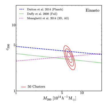
The best-fit model describes the data very well (Figure 6, Table 4). The two-halo term is an order of magnitude less than the NFW model, with an estimated halo bias of $b_{h}(M_{200})\simeq 5.5$. The point mass is constrained by the upper limit, $M_{\rm pt}<6.19\times 10^{11}\mathrel{h^{-1}M_{\odot}}$. The mass and the concentration at $\Delta=200$ (Figure 7) is in excellent agreement with both numerical simulations (Bhattacharya et al. 2013; Diemer & Kravtsov 2014; Meneghetti et al. 2014) and individual cluster mass measurements (Section 3.3). Okabe et al. (2013) conducted a similar stacked lensing analysis using a background galaxy catalogue based on a single colour cut, and based on the Ilbert et al. (2009) COSMOS photometric redshift catalogue. The stacked shear signal presented here is consistent with Okabe et al. (2013). The measurement uncertainties on the shear signal decrease as radius increases in this study due to radial dependence of our colour cut; this increases the weight of the outer bins in our fit, relative to that of Okabe et al. (2013). Therefore, the mass and concentration from our new stacked analysis are marginally higher and lower than Okabe et al. (2013) respectively.

We compare the stacked result at $\Delta=200$, shown in Table 4 with the lognormal mean of the individual cluster mass and concentration measurements listed in Table 3, finding excellent agreement, with the latter being $\langle M_{200}\rangle=6.38\pm 0.24\times 10^{14}\mathrel{h^{-1}M_{\odot}}$ and $\langle c_{200}\rangle=3.73\pm 0.38$.

We also divide the clusters into two sub-samples of 25 clusters based on the virial mass measured from the individual cluster shear profile models (Section 3.3), adopting $M_{\rm vir}=8\times 10^{14}\mathrel{h^{-1}M_{\odot}}$ as the dividing line between the sub-samples. We calculate the stacked shear profile for both sub-samples, and fit models, following the procedures applied to the full sample. The results are in excellent agreement with both numerical simulations (Bhattacharya et al. 2013; Diemer & Kravtsov 2014; Meneghetti et al. 2014) and the best-fit mass-concentration relation for individual cluster mass measurements (Table 3 & 4; Figure 7).

Figure 8: Mass-concentration relation (left) and $\alpha$-mass relation (right) for the Einasto profile obtained by the stacked lensing analysis. The cross denotes the best-fit parameters and the contours show the 68.3%, 95.4%, and 99.7% confidence levels. Left : blue dashed, green dotted and magenta dashed-dotted lines denote the mass-concentration relation derived by Dutton & Macciò (2014),Duffy et al. (2008), and Meneghetti et al. (2014), respectively. Right: blue dashed and green dotted lines are the $\alpha$-mass relation from Dutton & Macciò (2014) and Gao et al. (2008), respectively.

Some numerical simulation indicate that an Einasto (1965) profile describes the spherically averaged mass density profile for simulated halos better than the NFW profile (Navarro et al. 2004; Gao et al. 2012; Klypin et al. 2014). The Einasto profile has the form:

$$\frac{d\log\rho}{d\log r}=-2\left(\frac{r}{r_{-2}}\right)^{\alpha},$$ (32)

where $r_{-2}$ is a scale radius at which the logarithmic slope is $-2$ and $\alpha$ is a shape parameter to describe the degree of curvature of the profile. The Einasto profile is specified by three parameters of $M_{\Delta}$, $c_{\Delta}=r_{\Delta}/r_{-2}$ and $\alpha$. We measure these three parameters by fitting the stacked lensing profile for all 50 clusters. As demonstrated by the NFW fitting, the contribution from the point mass is negligible compared to that of the main halo in the radial range $0.1-2.8\mathrel{h^{-1}{\rm Mpc}}$. We therefore just fit the Einasto profile and two-halo term. The best-fit parameters are $\alpha=0.161_{-0.041}^{+0.042}$, $M_{200}=6.49_{-0.29}^{+0.31}\times 10^{14}\mathrel{h^{-1}M_{\odot}}$ and $c_{200}=3.26_{-0.54}^{+0.39}$. These constraints on $M_{200}$ and $c_{200}$ are in excellent agreement with the NFW-based measurements (Table 4), and also agree within $\sim 1\sigma$ with predictions from numerical simulations (Figure 8); Duffy et al. 2008; Gao et al. 2012; Bhattacharya et al. 2013; Diemer & Kravtsov 2014; Meneghetti et al. 2014). As noted above, the agreement between our results and the predictions from 2013-2014 is excellent. More precise observational constraints on the density profile shape of clusters, including mass dependence of the Einasto profile parameters await larger cluster samples, for example from the Dark Energy Survey (DES), Hyper Suprime-Cam survey (HSC) and the Large Synoptic Survey Telescope (LSST).

4 Discussion

In Section 4.1 we quantify the remaining systematics in our analysis, in Section 4.2 we summarize our overall error budget, and in Section 4.3 we compare our mass measurements with results from the literature.

4.1 Systematics

In Section 4.1.1 we test the methods described in Section 3.1 and that we use in Section 3.2 to fit NFW models to the observed shear profiles. In Section 4.1.2 we correct the shear signal for the small colour selection and galaxy shape measurement biases calculated in Sections 2.4 & 2.7 and re-fit the NFW models to the corrected shear profiles. In Section 4.1.3 we calibrate the impact of using the full photometric redshift probability distribution of the background galaxies on our mass measurements. In Section 4.1.4 we consider the impact of forcing the number density profile of background galaxies to be flat. (We emphasize again that in our analysis and results we do not assume the number density profile to be flat.)

4.1.1 Simulation Tests

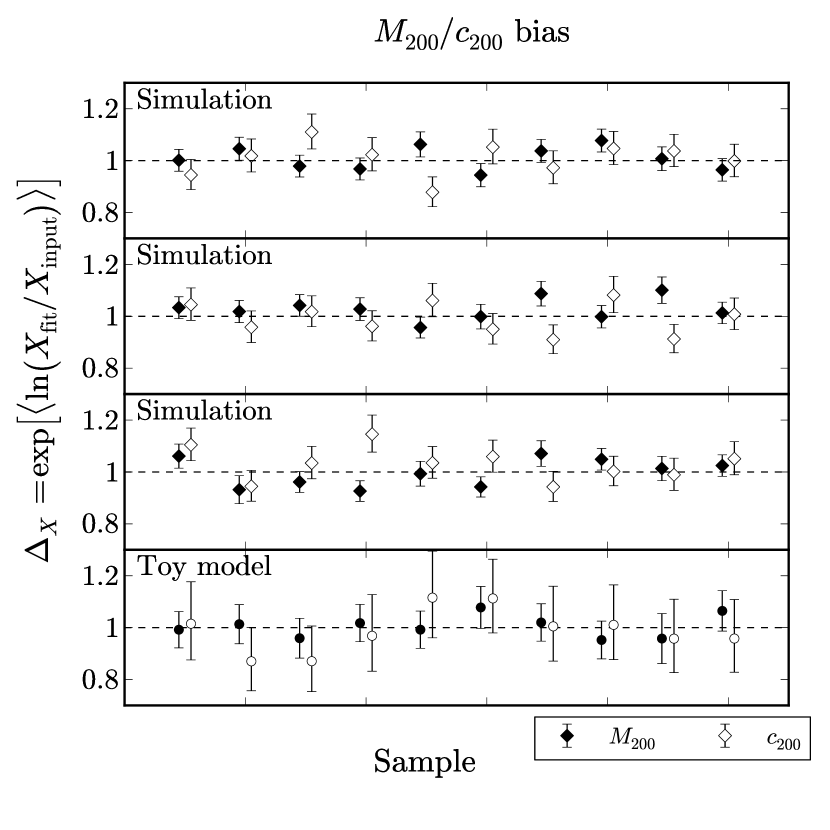
The radial range over which recent cluster weak-lensing studies (e.g. Israel et al. 2012; Melchior et al. 2014; Applegate et al. 2014; Hoekstra et al. 2015) have modeled the shear profile has been motivated in part by results from numerical simulations. Here, we expand upon Okabe et al. (2013), to test our individual mass measurements (Section 3.2) using synthetic weak shear catalogues based on simulated clusters and toy models. The former have the advantage of incorporating the full effects of the large-scale structure that surrounds massive clusters, whilst the latter have the advantage of toy model clusters having perfectly known properties, and the properties of the background galaxy catalogues are matched to the observational data. Importantly, we calibrate the specific model fitting method that we apply to our observational data directly on simulations whose properties match our own sample and data.

We use mock observations of clusters from the “Cosmo-OWLS” cosmological hydrodynamical simulation that reproduces a large number of local galaxy cluster scaling relations, within a $400\mathrel{h^{-1}{\rm Mpc}}$ box (Le Brun et al. 2014; McCarthy et al. 2014). We use the simulations that include cooling, star formation, supernova feedback and AGN feedback with a heating temperature $\Delta T_{\rm heat}=10^{8}$K, known as the AGN 8.0 model. Weak-lensing catalogues comprising 100 galaxies per ${\rm arcmin}^{2}$ were constructed following Bahé, McCarthy & King (2012). Specifically, the mock observations include the effect of shape noise, cluster substructure and triaxiality, and correlated large-scale structure, and ignore uncorrelated large-scale structure and observational effects such as uncertainties in galaxy shape measurements and redshifts. Note that ignoring uncorrelated large-scale structure is not expected to affect the measurement of possible biases in mass measurements via tests such as those described here (Hoekstra et al. 2011). The mass of the simulated clusters spans $5\times 10^{14}h_{73}^{-1}M_{\odot}<M_{200}<17\times 10^{14}h_{73}^{-1}M_{\odot}$ at a redshift of $z_{l}=0.23$ with the WMAP7 cosmology of $\Omega_{m,0}=0.272$ and $\Omega_{\Lambda}=0.728$. We randomly extracted galaxies from the parent synthetic weak shear catalogues to match statistically the cluster-centric number density profiles of colour-selected background galaxies in the observational analysis (Section 2.7), and fitted NFW models to the shear profiles following exactly the procedure laid down in Sections 3.1 & 3.2. This was repeated for 30 realizations, each containing 23 simulated clusters.

To quantify the mass measurement, we define $\Delta_{X}$ in terms of the geometric mean: $\Delta_{X}=\exp\left(\langle\ln(X_{\rm fit}/X_{\rm input})\rangle\right)-1$, following Umetsu et al. (2014), and similar to the methods of Becker & Kravtsov (2011). Here, $X_{\rm fit}$ is the best-fit mass or concentration. We recover the input $M_{200}$ and $c_{200}$ from the numerical simulations with negligible bias. The mean bias on the mass and concentration measurements across the full suite of realizations of the simulations is $\mathrel{\hbox{\hbox to0.0pt{\hbox{\lower 4.0pt\hbox{$\sim$}}\hss}\hbox{$<$}}}1$ per cent. The scatter between measurements of the bias on mass using individual realizations is $4.8$ per cent, which is comparable with the measurement uncertainty of $4.4$ per cent on the bias from an individual realization. Likewise the realization-to-realization scatter in bias on concentration is $6.2$ per cent, with a typical measurement uncertainty on an individual realization of $6.3$ per cent (upper three panels of Figure 9).

We repeat this test using cluster density profile models based on analytic NFW halos, and construct synthetic background galaxy catalogues that match the observed catalogues as closely as possible. For each of 50 analytic cluster profiles we adopt the observed positions of background galaxies and randomly draw a galaxy from the full background galaxy sample across all 50 clusters, thus simultaneously randomising the galaxy orientations, and matching statistically the source redshift distribution. The NFW parameters are randomly chosen from the measured values for our cluster sample. We compute the synthetic shear profile for each of these 50 analytic clusters 10 times and fit an NFW model following the procedures laid down in Sections 3.1 & 3.2. Again, we recover the input masses and concentrations with $\mathrel{\hbox{\hbox to0.0pt{\hbox{\lower 4.0pt\hbox{$\sim$}}\hss}\hbox{$<$}}}1$ per cent bias. The scatter between realizations is $4.3$ and $8.9$ per cent on mass and concentration respectively, and the typical measurement uncertainty on individual realizations is $7.7$ and $14.5$ per cent on mass and concentration respectively (lowest panel of Figure 9).

In summary, we conclude that our shear profile fitting algorithm, a key feature of which is the adaptive choice of binning scheme, recovers the mean mass of our sample with negligible bias.

Figure 9: Calibration tests for weak-lensing mass measurements ($M_{200}$,$c_{200}$). The top three panels and the bottom panel represent the results based on the numerical simulations (diamonds McCarthy et al. 2011; Bahé, McCarthy & King 2012, ; 23 clusters) and the toy models (circles; 50 clusters), respectively. The filled and open symbols denote the geometric means for the mass and the concentration, respectively.

4.1.2 Shear Calibration and Background Selection

In Sections 2.4 & 2.7 we developed methods to measure the shape of faint galaxies and select faint red galaxies as background galaxies with small systematic biases of $3$ and $1$ per cent respectively; both acting in the sense that we slightly under-estimate cluster mass. Here we estimate how these biases propagate through to the actually cluster mass measurements.

The shape measurement bias is expressed as the multiplicative shear calibration factor, $m=-0.03$, following the STEP programme. Given $m$, we therefore correct the measured tangential shear signal by $\Delta\Sigma_{+}\rightarrow\Delta\Sigma_{+}(1+m)^{-1}$ and repeat the tangential shear fitting described in Section 3.1. We express the comparison between the original masses (Table 2) and the corrected masses we define $\Delta_{M}$ in terms of the geometric mean: $\Delta_{M}=\exp\left(\langle\ln(M_{\Delta}^{\rm orig}/M_{\Delta}^{{\rm corr}})\rangle\right)-1)$. We find that the corrected masses are $\sim 3-5\%$ higher than the original masses, the range of values reflecting the non-linearity of tangential shear profiles (Table 5).

Turning to the colour selection of background galaxies, the right panel of Figure 3 shows that the contamination levels are $1$ per cent at $r\lower 2.15277pt\hbox{$\;\buildrel<\over{\sim}\;$}1.3\mathrel{h^{-1}{\rm Mpc}}$ and well below this level at $r\lower 2.15277pt\hbox{$\;\buildrel>\over{\sim}\;$}1.3\mathrel{h^{-1}{\rm Mpc}}$. We therefore boost the shear signals at $r\lower 2.15277pt\hbox{$\;\buildrel<\over{\sim}\;$}1.3\mathrel{h^{-1}{\rm Mpc}}$ and re-derive the cluster masses, again following Section 3.1. Expressing the comparison in the same manner as above, we found that the masses corrected for contamination are within $\mathrel{\hbox{\hbox to0.0pt{\hbox{\lower 4.0pt\hbox{$\sim$}}\hss}\hbox{$<$}}}1$ per cent of the original masses (Table 5).

For completeness, we combine these two shear correction terms in quadrature to give an effective multiplicative bias of $m=-0.032$, and evaluate the mass measurement bias of the combined shear calibration and contamination effects. As expected, the bias is mainly attributed to the shear calibration, with the combined correction yielding results indistinguishable from the pure shear calibration correction. Individual cluster masses based on the corrected tangential shear profile are given in Appendix B.

4.1.3 Mass Estimates with photometric redshift P(z)

Figure 10: A comparison of the mass (left) and the concentration (right) at $\Delta=200$, estimated by the single redshift, ($z_{s}$; Section 3.2) and the probability density function ($P(z)$; Section 4.1.3).

In Section 2.6 we adopted as the redshift of each faint galaxy in our sample, the median of the stacked posterior probability distribution of the nearest 100 neighbours in the $(V-i)-i$ space of the COSMOS catalogue. We therefore essentially adopted a point estimate of the redshift of each of our galaxies. However it is well known that the photometric redshift probability distribution of galaxies can be asymmetric, and present multiple peaks. The full photometric redshift probability density function, $P(z)$, fully describes such implicit systematic uncertainties. Indeed some recent studies have used the full $P(z)$ for some clusters in their weak-lensing sample (e.g. Applegate et al. 2014).

Here, we test whether our method that ignores the full $P(z)$ available from the COSMOS survey suffers any significant bias. In a similar vein to Section 2.6, we estimate the full $P(z)$ probability function of individual galaxies as an ensemble average of $P^{\rm COSMOS}(z)$ for 100 neighbouring COSMOS galaxies in the colour-magnitude plane,

$$P(z)=\frac{1}{N_{\rm nei}}\sum_{j}^{N_{\rm nei}}P_{j}^{\rm COSMOS}(z).$$ (33)

Given the probability function, the tangential shear component can then be calculated as follows:

$$\langle\Delta\Sigma_{+}\rangle(r_{i})=\frac{\sum_{n}\int_{z_{l}}^{\infty}g_{+,n}\Sigma_{\rm cr,n}(z_{s})w_{n}(z_{s})P(z_{s})dz_{s}}{\sum_{n}\int_{z_{l}}^{\infty}w_{n}(z_{s})P(z_{s})dz_{s}}.$$ (34)

The errors for the shape noise ($C_{g}$) and the photometric redshift ($\tilde{C}_{s}$) are estimated as:

$$C_{g,ij}=\frac{1}{2}\frac{\sum_{n}\int_{z_{l}}^{\infty}\sigma_{g,n}^{2}\Sigma_{\rm cr,n}^{2}(z_{s})w_{n}^{2}(z_{s})P(z_{s})dz_{s}}{(\sum_{n}\int_{z_{l}}^{\infty}w_{n}(z_{s})P(z_{s})dz_{s})^{2}}\delta_{ij},$$

and

$$\tilde{C}_{s,ij}=\frac{\sum_{n}\int_{z_{l}}^{\infty}(g_{+,n}\Sigma_{\rm cr,n}(z_{s})w_{n}(z_{s})-\langle\Delta\Sigma_{+}\rangle)^{2}P(z_{s})dz_{s}}{\sum_{n}\int_{z_{l}}^{\infty}P(z_{s})dz_{s}}\delta_{ij},$$

respectively.

We select the same background galaxies used in our main analysis and compute the tangential shear profiles using Equation (34). The radial bins are chosen using the same method as in our main analysis. The difference in the tangential shear components estimated by the single source redshift and $P(z)$ is calculated using:

$$\Delta_{+}^{2}=\frac{1}{N_{\rm bin}}\sum_{i}\frac{(\langle\Delta\Sigma_{+}^{z_{s}}\rangle-\langle\Delta\Sigma_{+}^{P(z)}\rangle)^{2}}{(\sigma_{+}^{z_{s}})^{2}+(\sigma_{+}^{P(z)})^{2}},$$ (35)

where $\sigma_{+}^{2}=C_{g}+\tilde{C}_{s}$. The deviation is, on average, $\Delta_{+}\simeq 0.05$, with smaller deviations of $\Delta_{+}\sim 0.02$ at small radii ($r<0.3\mathrel{h^{-1}{\rm Mpc}}$) and larger deviations of $\Delta_{+}\sim 0.07$ at large radii ($r>1\mathrel{h^{-1}{\rm Mpc}}$). This is because the errors at small radii are larger, due to a the relatively small number of background galaxies in bins of smaller solid angle. When we ignore the errors, the average deviations are still negligible, $\Delta_{+}\sim 0.01$ at $r<0.3\mathrel{h^{-1}{\rm Mpc}}$ and $\Delta_{+}\sim 0.002$ at $r>1\mathrel{h^{-1}{\rm Mpc}}$. We also compare the best-fit mass and concentration parameters (Figure 10). The two measurements are in excellent agreement, with geometric means of $0.97\pm 0.05$ and $0.96\pm 0.15$ for $M_{200}$ and $c_{200}$, respectively. We also made a background galaxy catalogue using the $P(z)$ function and our radius-dependent colour-cut (Section 2.7), and found that again the mass measurements do not change significantly ($0.96\pm 0.05$ and $0.96\pm 0.15$ for $M_{200}$ and $c_{200}$). We conclude that with the current sample and data we are unable to detect any systematic difference between the mass and concentration measurements based on the mean of COSMOS point estimates of the redshift of individual galaxies and the full COSMOS $P(z)$ function.

4.1.4 Boost factor

Figure 11: Systematic mass measurement errors caused by the boost factor. Left: the stacked tangential shear profiles. Back diamonds and green squares denote the profile computed by our background catalogue and galaxies with $\Delta C>0$, respectively. Blue crosses and red circles are the profile corrected by the boost-factor and the boost-factor taking into account the magnification bias, respectively. Middle: the differential fraction of lensing signals from the signals for our background catalogue. The lensing signal corrected by the boost factor, with the assumption of the uniform background distribution, is significantly underestimated. Right:the normalized number density profile. Green squares shows a clear excess of the density profile of galaxies with $\Delta C>0$. The best-fit model is represented by the dashed blue lines. The dotted red line denotes the depleted number density profile due to the magnification bias. The solid black line is the dilution model (Section 2.7). The dotted-dashed magenta line is the boost factor for MACS J0417.5$-$1154 from the WtG project (Applegate et al. 2014), showing a shallow distribution.

Imperfect selection of background galaxies leads to under-estimated weak-shear signals because background galaxy samples are contaminated by faint cluster galaxies, the shapes of which present no lensing signal due to the cluster. The number density of cluster galaxies decreases with increasing projected cluster-centric radius. Thus at fixed selection method, the ratio of cluster galaxies to background galaxies, $f_{\rm mem}$, decreases with increasing projected cluster-centric radius, and thereby dilutes the shear signal more at smaller radii than at larger radii. Our approach is to vary the colour cut used to select background galaxies as a function of cluster-centric radius, simply exploiting the declining number density of cluster galaxies as a function of radius, without invoking any physical assumptions. An alternative (e.g. Kneib et al. 2003; Applegate et al. 2014; Hoekstra et al. 2015) is to correct the measured shear signal by a factor $1+f_{\rm mem}$, and thus to assume that the observed number density profile of background galaxies is flat. This correction is referred to as a boost factor. However, the assumption of a flat observed number density profile of background galaxies ignores magnification bias (e.g. Broadhurst, Taylor & Peacock 1995; Umetsu et al. 2014) – i.e. the depletion or enhancement of the number density of background galaxies due to lensing magnification.

We compare the boost-factor method with our methods that do not invoke a boost factor and instead rely on selection of red galaxies to achieve $\leq 1$ per cent dilution across all radii. For this purpose, we construct background galaxy catalogues that suffer dilution by selecting red galaxies with a positive colour-offset from the red-sequence, $\Delta C>0$, and compute the stacked shear profile for this diluted sample of galaxies. As expected, the amplitude of this shear profile is suppressed relative to the shear profile from our main analysis, with the suppression increasing to $\sim 50\%$ at $\sim 100\mathrel{h^{-1}{\rm kpc}}$ from the cluster centre (left and central panels of Figure 11). The suppression of the signal due to dilution appears to be negligible at $\lower 2.15277pt\hbox{$\;\buildrel>\over{\sim}\;$}1\mathrel{h^{-1}{\rm Mpc}}$. The contaminating population of faint cluster galaxies is seen clearly as an excess of galaxies at $\mathrel{\hbox{\hbox to0.0pt{\hbox{\lower 4.0pt\hbox{$\sim$}}\hss}\hbox{$<$}}}1\mathrel{h^{-1}{\rm Mpc}}$ in the stacked number density profile of galaxies selected as having $\Delta C>0$ (right panel of Figure 11). In other words, the excess of number density profile is negligible beyond $r_{200}$. The evidence indicates an internal consistency that the number density excess and the stacked-lensing mass estimate are consistent with each other. Note that the number density profile in Figure 11 is calculated after masking the solid angle subtended by bright galaxies ($i^{\prime}<20$) out to elliptical radii a factor of $3$ than the elliptical shape parameters of SExtractor – i.e. corresponding to the isophotal limit of detected objects. We also fully consider the finite field-of-view in the number density calculation. To quantify the contaminating population we fit the function $f_{\rm mem}=A\exp\left(-r/r_{0}\right)$ to the measured number density profile (dashed blue curve in right panel of Figure 11). We use this model to boost the measured shear signal by a factor $1+f_{\rm mem}$ (blue crosses in left and central panels of Figure 11). It is clear that the boosted shear signal underestimates the lensing signal that we detect by $\sim 40\%$ on small scales, and $\mathrel{\hbox{\hbox to0.0pt{\hbox{\lower 4.0pt\hbox{$\sim$}}\hss}\hbox{$>$}}}10\%$ at all radii interior to $\sim 1\mathrel{h^{-1}{\rm Mpc}}$. Lens magnification is an obvious culprit for this apparent deficit of signal in the boost-factor-corrected shear profile.

The galaxy-count is depleted by the magnification bias, as expressed by

$$N(r;<m)=N_{0}(r;<m)\mu(r)^{2.5s-1},$$ (36)

where $\mu^{-1}=(1-\kappa)^{2}-|\gamma|^{2}$ is the lensing magnification which expands the area of sky and enhances the flux of galaxies, and $s=d\log_{10}N_{0}(m)/dm$ is a logarithmic count slope. Given the best-fit mass model derived by the stacked shear analysis (Table 4), we calculate the number density profile expected from the magnification bias, assuming $s=0.15$ (Umetsu et al. 2014). This calculation shows clearly that the expected number density profile of background galaxies is not flat, showing a decline interior to $\sim 1\mathrel{h^{-1}{\rm Mpc}}$ (dotted red curve in right panel of Figure 11). This indicates that the assumption of a flat background galaxy number density profile is incorrect, even on scales comparable with $r_{500}$.

Next, we boost the $\Delta C>0$ shear profile (blue squares in left and central panels of Figure 11) by both the boost factor, and the expected number density profile of background galaxies from the magnification bias calculation discussed in the proceeding two paragraphs. This boost factor and magnification bias corrected shear profile comes closer to recovering our measured shear profile, although it remains $\sim 10\%$ lower interior to $\sim 1\mathrel{h^{-1}{\rm Mpc}}$ (red points in left and central panels of Figure 11). Clearly, the number density profile based on an imperfect background selection is tightly coupled with the dilution effect and the magnification bias. It is therefore very difficult to break the degeneracy between the dilution effect and the magnification bias using the imperfect background catalogue. We also mention that the boost-factor gives rise to systematics in the source redshift because member galaxies in background catalogue have inadequate redshifts. Overall, our analysis in this Section indicates that application of a boost factor without consideration of lens magnification may cause systematic biases even on quite large scales up to $\sim\,r_{500}$.

4.2 Error budget

Table 5: Systematic errors on the mean mass, $\langle M_{\Delta}\rangle$, for 50 clusters, in units of a percentage.

Name	expected	$M_{\rm vir}$	$M_{200}$	$M_{500}$	$M_{1000}$	$M_{2500}$
Shear calibration	$-3$	$-4.1$	$-4.2$	$-2.7$	$-4.8$	$-5.3$
Colour selection	$-1$	$0.2$	$0.0$	$-0.5$	$-0.9$	$-1.7$
Shear+colour calibration	$-3.2$	$-4.1$	$-4.2$	$-2.7$	$-4.8$	$-5.3$
Radial bins	$-$	$\pm 0.9$	$\pm 1.0$	$\pm 1.4$	$\pm 2.3$	$\pm 4.4$

We summarize the contributions to our overall error budget. The largest systematic bias in our measurements is caused by imperfections in our faint galaxy shape measurements, with a STEP-like multiplicative bias of $m\simeq-0.03$ that is independent of galaxy size. We tuned our faint galaxy selection method to yield a contamination level of $\leq 1$ per cent, thus again giving a very small systematic bias. This low level of contamination renders the background galaxy samples essential pure, and thus not requiring correction. Nevertheless, for completeness, we correct the shear profiles for these two bias terms and obtain “corrected masses” (see Appendix) that are $\sim 3-5$ per cent higher than the “uncorrected masses” in Table 2. In particular, after correction, our measurements of $M_{500}$ increase by just $2.7$ per cent on average.

We have also investigated several other errors, none of which contribute to systematic biases. First, the typical uncertainty on the distance ratio $D_{ls}/D_{s}$ for each individual background galaxy, computed from the COSMOS photometric redshift catalogue following the methods described in Section 2.6 is $\sigma_{\beta}\simeq 13-28$ per cent. These uncertainties are included in the covariance matrix when fitting the NFW model to the respective shear profiles (Section 3.1). Second, when exploring different shear profile binning schemes, and applying them to the observational shear measurements, we found that the $M_{500}$ values for individual clusters scatter by $\pm 1.4$ per cent. Third, when applying our shear profile binning scheme to simulated data we recovered the true masses with $\mathrel{\hbox{\hbox to0.0pt{\hbox{\lower 4.0pt\hbox{$\sim$}}\hss}\hbox{$<$}}}1$ per cent bias and $\sim 5$ per cent scatter between different realizations of the simulations (Section 4.1.1). Fourth, we tested whether using a point estimator of the photometric redshift of a galaxy in the COSMOS catalogue introduced any systematic bias with respect to using the full $P(z)$ distribution. We found that the latter yields masses $4\pm 6$ per cent lower than the former. Given the poor precision to which have been able to measure this possible bias, we ignore it here. However this deserves more detailed investigation in future larger surveys. Whilst we have sought to minimize the assumptions in our analysis pipeline, we would like to draw attention to the dependence of our results on the COSMOS field. We have assumed that the galaxy population probed by observations of this field are representative of the universe as a whole. This assumption is relevant to the shera-based shape measurement tests described in Section 2.5, and aspects of our analysis that rely on the COSMOS photometric redshift distribution (Sections 2.6 & 2.7). Several many-filter and deep COSMOS-like calibration fields would be very beneficial for future deep and wide lensing surveys including LSST.

4.3 Comparison of mass measurements with the literature

Figure 12: Mass comparisons of different projects: the top-left (Ok10; Okabe et al. 2010a), top-right (CCCP Hoekstra et al. 2015), bottom-left (CLASH Umetsu et al. 2014) and bottom-right (WtG Applegate et al. 2014). Masses are measured at the same radii in order to avoid the aperture-induced errors. The mass ratios for the overlap sample are computed by the geometric means.

Table 6: Comparison with previous studies, $M_{\rm pre}(<r_{\Delta}^{\rm pre})/M_{\rm LoCuSS}(<r_{\Delta}^{\rm pre})$. All masses are the NFW spherical masses measured within the overdensity radii $r_{\Delta}$ defined by previous studies (Ok10,CCCP, CLASH and WtG) or $1.5h_{70}^{-1}\mathrel{\rm Mpc}$, in order to avoid the aperture-induced-errors in the mass estimates. We also summarize the mass-measurement method and approach to correction of biases for each project. “Method” denotes the tangential shear fitting ($g_{+}$) and a joint fitting using tangential shear profiles and the magnification bias ($g_{+}$ & $\mu$). “Calibration factor” is the shear-calibration factor, with “Yes” indicating that such a factor was applied to the shear signal before fitting mass models, and “No” indicating otherwise. “Boost factor” is the correction factor by the number density caused by imperfect background selection – Yes/No indicates whether or not this factor was calculated and applied to the data. $c_{\Delta}$ states whether the concentration parameter was a free parameter in the fit, or fixed, or scaling with the mass. “Radial bins” gives the choice of radial binning scheme for the fitting of the shear profile. “N” is the number of clusters in common between this study and each of the other studies.

Name	Method	Calibration	Boost	Radial	$c_{\Delta}$	N	Virial	$200$	$500$	$2500$	$1.5h_{70}^{-1}$Mpc
		factor	factor	bins
This paper	$g_{+}$	No	No	Adaptive	Free	$-$	$-$	$-$	$-$	$-$	$-$
Ok10	$g_{+}$	No	No	Fixed	Free	20	$0.81\pm 0.07$	$0.82\pm 0.06$	$0.85\pm 0.05$	$0.91\pm 0.08$	$-$
CCCP	$g_{+}$	Yes	Yes	Fixed	Scaling	21	$0.94\pm 0.06$	$-$	$0.95\pm 0.06$	$0.97\pm 0.07$	$-$
CLASH	$g_{+}$ & $\mu$	Yes	No	Fixed	Free	5	$0.99\pm 0.14$	$1.02\pm 0.13$	$1.07\pm 0.12$	$-$	$1.03\pm 0.10$
WtG	$g_{+}$	Yes	Yes	Fixed	Fixed	17	$-$	$1.14\pm 0.09$	$1.16\pm 0.12$	$1.17\pm 0.14$	$1.15\pm 0.07$

Ongoing projects, including LoCuSS, CCCP (Hoekstra et al. 2015), CLASH (Umetsu et al. 2014) and WtG (Applegate et al. 2014), conducted cluster weak-lensing analyses. Comparison of the cluster mass measurements between these different surveys is of paramount importance for cluster cosmology experiments. There are important differences between the approach taken by each survey to the cluster mass measurements. For example, CCCP and WtG implement the boost factor method (Section 4.1.4) to correct their shear signal. Another key difference is the prior adopted on the concentration parameter of the NFW halo model that is fitted to the data. For example, WtG fix the concentration parameter at $c_{200}=4$, whilst we allow it to be a free parameter in our fits. We summarize the key differences between the respective analysis methods in Table 6, and highlight key points in the following sections. Throughout these sections, when we compare cluster masses between two surveys we do so within the same radii so as to avoid errors caused by aperture mis-match. Also, all comparisons are done without applying the colour-selection and shear-calibration corrections to our shear measurements, discussed in Section 4.1.2.

4.3.1 LoCuSS – Okabe et al. (2010)

Okabe et al. (2010a) conducted weak-lensing analysis for 30 clusters using Suprime-Cam data. As some of clusters lacked $V-$ band data, we measured masses only for 22 clusters, defining as background galaxies those galaxies with colours are redder or bluer than those of the red-sequence. The red and blue colour cuts were chosen by eye based on the run of lensing signal with colour offset from the red sequence. We didn’t adopt any correction factor inherent in the shear calibration and the profiles of the background number density. The error on the tangential shear measurements only took into account shape noise. We treated the mass and the concentration as free parameters when fitting the NFW model to the tangential shear profiles. The masses derived from our new analysis presented in this article are $20\%$ to $9\%$ higher than obtained in 2010, with larger differences found for masses measured in larger radii (Table 6; Figure 12). Our previous mass measurements were under-estimated due to issues in shear calibration and imperfect background galaxy selection.

4.3.2 CCCP – Hoekstra et al. (2015)

The Canadian Cluster Comparison Project (CCCP Hoekstra et al. 2015) carried out weak-lensing mass measurement for 52 clusters using the Canada-France-Hawaii Telescope (CFHT). Their sample is defined by clusters with an ASCA temperature of $k_{B}T_{X}>5\,{\rm keV}$ in the range of $0.15<z<0.55$. They used $B-$ and $R-$ bands for the first 20 clusters with the CFH12k camera and $g^{\prime}-$ and $r^{\prime}-$ bands for the other 32 clusters with the Megacam (hereafter we refer to the redder band as $r$-band for both instruments). They used solely their $r$-band data to select galaxies at $22<r<25$ as background galaxies. The number density profile of these galaxies was found to increase towards the cluster centres. Hoekstra et al. modelled this excess of galaxies on a cluster-by-cluster basis, and boosted the lensing signals by a factor of $1+f_{\rm contam}(r)$ assuming a flat background number density profile of background galaxies, where $f_{\rm contam}(r)$ is the fraction of contaminating galaxies obtained from their models. This boost factor increases their masses by $1-2$ per cent. They adopt the mass-concentration relation (Dutton & Macciò 2014) for their mass estimates.

There are 21 clusters in common between the CCCP and LoCuSS samples. On average, the CCCP masses are $\sim 3\%-6\%$ lower than our masses (Table 6; Figure 12), however this difference is not statistically significant. We note that the radial range of their model fits is $0.5-2h_{70}^{-1}{\rm Mpc}$ – i.e. it includes scales on which we expect the magnification bias to affect the slope of the number density profile of background galaxies (Figure 11; see also Ziparo et al. 2015). Nevertheless, we see good agreement between LoCuSS and CCCP mass measurements.

4.3.3 CLASH – Umetsu et al. (2014)

The Cluster Lensing And Supernova survey with Hubble (CLASH; Umetsu et al. 2014) conducted a joint shear-and-magnification weak-lensing analysis of a sample of 20 galaxy clusters at $0.19\lower 2.15277pt\hbox{$\;\buildrel<\over{\sim}\;$}\,z\lower 2.15277pt\hbox{$\;\buildrel<\over{\sim}\;$}0.69$, using imaging through multiple filters with Subaru/Suprime-Cam. They measure galaxy ellipticities using the KSB$+$ method, and calibrate the isotropic PSF correction for galaxies detected with high signal-to-noise ratio – i.e. using methods similar to our own. They also employ a correction factor $1/0.95$ to account for residual shear calibration. Background galaxies are selected in a colour-colour plane, typically based on the $B_{J}R_{C}z^{\prime}$-band filters, following Medezinski et al. (2010). They do not employ a boost factor to compensate for contamination of their background galaxy catalogues. The halo concentration for the NFW model is treated as a free parameter. We compare the CLASH and LoCuSS masses for 5 clusters in common, obtaining excellent agreement (Figure 12 and Table 6). Recently, Umetsu et al. (2015) have published joint strong plus weak-lensing mass measurements of the CLASH sample. Their strong+weak-lensing masses are in a similar excellent agreement with our measurements.

4.3.4 WtG – Applegate et al. (2014)

The Weighing the Giants programme (WtG; Applegate et al. 2014) have conducted weak-lensing mass measurements for 51 X-ray luminous galaxy clusters in the redshift of $0.15\lower 2.15277pt\hbox{$\;\buildrel<\over{\sim}\;$}z\lower 2.15277pt\hbox{$\;\buildrel<\over{\sim}\;$}0.7$, using data from Subaru/Suprime-Cam. They calibrated their shape measurement pipeline using the STEP simulations and used this calibration to correct their faint galaxy shape measurements down to 25th magnitude. Note that their shape measurements suffered significant noise bias at fainter magnitudes. We compare our masses with WtG masses based on colour-selected galaxies, and therefore concentrate further discussion of their methods on those measurements.

WtG define two catalogues of background galaxies to compute tangential shear profiles. The first catalogue is used to calculate the contamination correction, namely the boost factor, which is shown by blue points in Figure 4 of Applegate et al. (2014), and the second catalogue is used to compute the tangential shear profile represented by orange points in the left panel of their Figure 4. The first catalogue is defined by employing magnitude and size cuts and exclusions of stars and galaxies that lie on the red-sequence of cluster galaxies. They found an apparent excess in the number density profiles at small radii because of imperfect background selection. The excess is described by $f_{\rm mem}(r)=N_{\rm mem}/(N_{\rm mem}+N_{\rm bkg})=f_{500}\exp(1-r/r_{500,X})$ which is the ratio of the member galaxies divided by the total number (member and background) of galaxies selected. Here, they assume a constant number density profile of background galaxies, and thus ignore the potential effects of magnification bias. All clusters are fitted simultaneously to estimate $f_{500}$ and $r_{500,X}$. The normalization $f_{500}$ for the first catalogue is $(8.6\pm 0.9)\%$. Figure 4 in Applegate et al. (2014) shows that $r_{500,X}\sim 1.4-2h_{70}^{-1}{\rm Mpc}$ which is very large. For example, Martino et al. (2014) obtain a median of $r_{500,X}\simeq 1h_{70}^{-1}{\rm Mpc}$ and values in the range $0.8-1.6h_{70}^{-1}{\rm Mpc}$ for the same sample that we study here, that has considerable overlap with the WtG sample. Whilst cluster-by-cluster comparison of $r_{500,X}$ measurements is required to be certain, the large values of this parameter used by WtG suggests that they assume a rather shallow radial density distribution when they model contamination of the background galaxy samples (right panel of Figure 11). Their shallow number density profile indicates that cluster members are distributed beyond the cluster virial radii, which conflicts with our results that the number density of cluster members is negligible in these regions (Section 4.1.4). Their number density result therefore appears to be inconsistent with their weak-lensing mass measurements. The shallow number density profile found by the WtG may therefore be a source of systematic bias in their mass measurements.

Next, they draw the second catalogue from the first catalogue with additional conditions of robust shape measurements and lensing cut ($S/N>3$ and $r_{h}>1.15r_{h}*$). The tangential shear profile is computed from the second catalogue. The excess of the number density profile, $f^{\prime}_{500}=4.8\pm 1.6\%$, is less than that obtained by the first catalogue. The tangential shear profile using the second catalogue is corrected by the boost factor that was calculated using the first catalogue. We here explicitly describe their definition of the corrected lensing signal, as follows, $g_{+}^{\rm 2nd}\rightarrow g_{+}^{\rm 2nd}/(1-f_{\rm mem}^{\rm 1st}(r))$. Here, 1st and 2nd denotes the quantities computed by the first and second catalogues, respectively. This inconsistency may affect the precision of the WtG mass measurements.

We emphasize that the boost factor cannot recover the correct lensing signal because of the magnification bias, as demonstrated in Sections 2.7 and 4.1.4, notwithstanding the fitting range, $0.75-3h_{70}^{-1}{\rm Mpc}$, that WtG adopt. Finally, they assumed $c_{200}=4$ for the NFW model for all clusters at all redshifts. Numerical simulations (e.g. Bullock et al. 2001; Duffy et al. 2008; Bhattacharya et al. 2013; Diemer & Kravtsov 2014; Meneghetti et al. 2014; Ludlow et al. 2014) show that the concentration depends on both the halo mass and redshift.

WtG masses are $\sim 15\%$ higher than our masses, independent of overdensity, albeit at $\sim 1-2\sigma$ significance (Table 6; Figure 12). Note that we exclude A1758N from this comparison because the WtG adopt a radial fit range that extends into the companion cluster A1758S. When we follow the WtG method – i.e. restrict the radial range of the fit to $0.75-3\,h_{70}^{-1}{\rm Mpc}$ and adopt $c_{200}=4$, the statistical significance of the disagreement increases slightly, with geometric means at $\Delta=200,500,2500$ and $1.5\,h_{70}^{-1}{\rm Mpc}$ of $1.18\pm 0.09$, $1.19\pm 0.12$,$1.19\pm 0.14$, and $1.18\pm 0.07$, respectively. We note that the difference between our mass measurements and those of WtG is significant at $\mathrel{\hbox{\hbox to0.0pt{\hbox{\lower 4.0pt\hbox{$\sim$}}\hss}\hbox{$>$}}}2\sigma$ on the scale preferred by WtG, $1.5\,h_{70}^{-1}\mathrel{\rm Mpc}$.

In summary, we have identified several strong assumptions and inconsistencies in the WtG analysis: the inconsistent calculation for the boost factor, the shallow number density profile leading to high boost factor, ignoring the magnification bias, and the fixed concentration $c_{200}=4$. We expect that the tension between our respective mass measurements will be caused by one or more of these issues.

4.3.5 CCCP, WtG and LoCuSS

Figure 13: Mass comparisons for 12 cluster overlapped among the three projects of CCCP(Hoekstra et al. 2015), WtG (Applegate et al. 2014) and LoCuSS. Masses are measured at $1.5h_{70}^{-1}$Mpc, derived by the WtG fitting method; the radial range is $0.75-3\,h_{70}^{-1}$Mpc and $C_{200}=4$. The bottom panel shows a comparison of CCCP masses (red diamonds) and WtG masses (blue circles). The top panel shows individual masses of 12 clusters. Red diamonds, green squares and blue circles denote CCCP, LoCuSS and WtG masses, respectively.

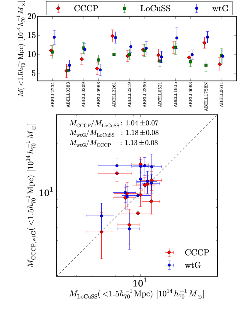
The cleanest comparison between surveys is between the respective mass measurements for 12 clusters in common between all of CCCP (Hoekstra et al. 2015), WtG (Applegate et al. 2014) and LoCuSS (this article). We follow the WtG fitting method, that is, we fix the NFW model concentration parameter at $c_{200}=4$, and fit the NFW model to the observed shear profile in the radial range is $0.75-3h_{70}^{-1}$Mpc. We compare three spherical NFW masses within $1.5h_{70}^{-1}$Mpc. Based on these conditions, the mass comparison approximately corresponds to a comparison of lensing signal at the fixed radial range. This like-for-like comparison confirms the results discussed in the preceding sections: for the subsamples of clusters in the LoCuSS sample that have also been studied by CCCP and WtG, the CCCP and LoCuSS masses are in good agreements with each other, while the WtG masses are $\sim 2\sigma$ higher than both CCCP and LoCuSS masses (Figure 13).

4.3.6 Sensitivity of conclusions to “sample selection”

An important caveat on the conclusions discussed in Sections 4.3.2–4.3.5 is that they are strictly only applicable to the specific sub-samples of clusters that have been observed by other surveys that are in common with our sample. We therefore consider whether our conclusions are supported by inter-survey comparisons in the literature – i.e. by comparison of masses of clusters in the overlap between other pairs of surveys, thus excluding our LoCuSS sample selection and mass measurements from the discussion.

Hoekstra et al. (2015) find that WtG masses from Applegate et al. (2014) are $\sim 6-8$ per cent higher than their CCCP measurements at $\sim 2\sigma$ significance, depending on the redshift distribution adopted by the two surveys. This is consistent with our conclusions, however it is intriguing to note that WtG masses agree very well with CCCP masses when the latter are computed by deprojecting aperture mass estimates. Hoekstra et al. also compare their mass measurements with CLASH measurements of 6 clusters in common between these surveys, finding that CLASH masses from Umetsu et al. (2014) exceed CCCP masses by $12\pm 5$ per cent. Umetsu et al. (2015) also find similar results (a $16\pm 10$ per cent excess) for five clusters in common between their joint strong plus weak-lensing analysis of the CLASH sample and the Hoekstra et al. weak-lensing masses. The CCCP/CLASH comparison appears to be at odds with our finding that CLASH, CCCP, and LoCuSS are all consistent, and underlines our caveat that conclusions based on mass comparison between surveys may be sensitive to the specific overlapping sub-samples considered. However, the overlap between CLASH and WtG numbers 17 clusters, i.e. a number of clusters comparable with the LoCuSS/CCCP and LoCuSS/WtG samples discussed in Sections 4.3.2 & 4.3.4. Both Umetsu et al. (2014) and Umetsu et al. (2015) find that WtG masses exceed the CLASH masses by $\sim 7-10$ per cent, albeit at $\sim 1\sigma$ significance.

In summary, a consistent picture emerges from comparisons between LoCuSS, CLASH, CCCP, and WtG surveys when the samples in common between the surveys number $\mathrel{\hbox{\hbox to0.0pt{\hbox{\lower 4.0pt\hbox{$\sim$}}\hss}\hbox{$>$}}}10$ objects: the WtG cluster mass calibration exceeds that of other surveys by $\sim 6-15$ per cent at $\sim 1-2\sigma$ significance per pair of surveys considered. Further inter-comparison of mass measurements based on all of the methods used by the respective surveys, preferably using an enlarged and common sample of clusters, should help to clarify the remaining differences between the surveys.

5 Summary

We observed an almost complete $L_{X}$-selected sample of 50 galaxy clusters at $0.15<z<0.3$ through $V$- and $i^{\prime}$-band filters with the Suprime-CAM instrument on the Subaru 8.2-m telescope. We used these data to measure the weak gravitational shear signal, and thus to infer the total mass and concentration of each cluster, and the sample as a whole via a stacking analysis. The size of our sample and typical statistical precision on weak-lensing mass measurements of $30$ per cent motivates our goal of controlling systematic biases in our analysis at the $\sim 30/\sqrt{50}\simeq 4$ per cent level.

The recent literature identifies the dominant systematic uncertainty in weak-lensing analysis of cluster samples as contamination of background galaxy samples by faint cluster galaxies. We extend our background galaxy selection method based on the dependence of gravitational shear signal on the colours of galaxies (Okabe et al. 2013) to incorporate the empirical fact that, at fixed colour cut, contamination by faint cluster members is a declining function of clustercentric radius. This allows us to define colour cuts that are a function of clustercentric radius such that we achieve negligible contamination (we required $\leq 1$ per cent contamination) whilst achieving a number density of 13 galaxies per square arcminute. We stress that our approach to selecting background galaxies neither assumes a form for the cluster mass distribution nor assumes a radial distribution for the background galaxies. We show that this latter point is important because gravitational magnification modifies the observed radial distribution of background galaxies on scales as large as $\mathrel{\hbox{\hbox to0.0pt{\hbox{\lower 4.0pt\hbox{$\sim$}}\hss}\hbox{$>$}}}1\mathrel{h^{-1}{\rm Mpc}}$ from the cluster centres and thus complicates methods that assume the radial distribution of background galaxies is flat (see also Ziparo et al. 2015 for a detailed discussion).

The dominant systematic bias in our analysis is the accuracy of our faint galaxy shape measurements. We test our modified KSB$+$ method on large simulated datasets that incorporate smooth analytic galaxy templates based on Sersic profiles, and realistic galaxies based on high resolution imaging with the Hubble Space Telescope. The key feature of our shape measurement code is that we use a very high signal-to-noise ratio cut when selecting galaxies to model the isotropic PSF correction. The precision that we achieve in this model as a result of this cut is important because it significantly reduces the noise bias that is typically seen at faint flux levels in other studies (e.g. Applegate et al. 2014; Hoekstra et al. 2015). We show that our STEP-like multiplicative shape measurement bias is of order 3 per cent, and is not a strong function of apparent magnitude and galaxy size. This is the largest systematic bias that we have identified in our analysis.

Controlling contamination of our background galaxy sample at the per cent level across a wide range of clustercentric radii (down to $\sim 200\mathrel{h^{-1}{\rm kpc}}$) affords us the opportunity to fit for both mass and concentration parameter when modeling the weak shear signal. This is important because it eliminates the possibility of systematic biases caused by fixing the shape of the density profile or adopting a mass concentration relation from simulations. We are also interested in measuring the mass-concentration relation of cluster-scale dark matter halos. To further mitigate the possibility of biases when modeling the shear signal, we apply a range of binning schemes (number of bins, inner and outer fit radii) to the data that are well motivated by the physical properties of clusters and previous tests of weak-lensing methods (e.g. Meneghetti et al. 2010; Becker & Kravtsov 2011; Bahé, McCarthy & King 2012). For each cluster we adopt the mass and concentration measurement of the binning scheme that yields the measurements that are the closest to the mean of the measurements from the range of binning schemes that we explore. This is a new method, and thus we test it on simulations including full hydrodynamical numerical simulations from cosmo-OWLS (Le Brun et al. 2014; McCarthy et al. 2014), based on an AGN model that reproduces a large number of local X-ray-SZ-optical scaling relations. Our tests show that we recover the ensemble mass and concentration of the simulated systems with sub per cent accuracy and of order 5 per cent scatter between different realisations of the simulated lensing observations. Issues relating to the binning and modeling of the shear signal are therefore sub-dominant in our analysis.

We now summarise our main science results. We measured weak-lensing mass for individual clusters by fitting tangential shear profile with the spherical NFW model and investigated the mass-concentration relation. The best-fit mass-concentration relation is in excellent agreement with recent numerical simulations (Bhattacharya et al. 2013; Diemer & Kravtsov 2014; Meneghetti et al. 2014). We also measured the average mass density profile for the NFW and Einasto profiles by stacked lensing analysis, considering the point mass and the two-halo term. The best-fit NFW model of the stacked signal agrees well with the mean of the individual mass measurements, supporting that the stacked lensing analysis recover the average of individual mass measurements. The Einasto profile also agrees with numerical simulations, albeit large scatter between numerical simulations.

We compared our lensing masses with masses from other projects (CCCP, CLASH and WtG). The philosophy of weak-lensing analyses for the four projects include some strong differences. Our mass measurements agree within $1\sigma$ with the CLASH (Umetsu et al. 2014) and CCCP (Hoekstra et al. 2015) surveys, with whom we have 5 and 21 clusters in common respectively. Our mass measurements are $\sim 15$ per cent lower than WtG measurements for the 17 clusters in common, at $\sim 1-2\sigma$ significance, depending on the mass measurement aperture. The fairest comparison between CCCP, WtG and LoCuSS is for the 12 clusters in common between all three surveys and based on a common mass measurement aperture and assumption on density profile shape. Adopting $c_{200}=4$ and measuring mass within $1.5h_{70}^{-1}\mathrel{\rm Mpc}$ (i.e. matching to WtG), confirms that LoCuSS and CCCP mass calibrations are consistent with each other and WtG is in tension at $2\sigma$ higher mass than the other two surveys.

To guard against possible sensitivity of this conclusion to the specific samples under investigation here, we also reviewed recent studies in the literature that compare other pairs of surveys (and thus exclude LoCuSS). We find that WtG are in tension with masses $\sim 6-15$ per cent higher than other surveys at $\sim 1-2\sigma$ significance in all pairwise comparisons that include $\mathrel{\hbox{\hbox to0.0pt{\hbox{\lower 4.0pt\hbox{$\sim$}}\hss}\hbox{$>$}}}10$ objects. We discuss a range of possible causes of this tension, including strong assumptions on the radial distribution of background galaxies and the halo concentration parameter, and several inconsistencies in the construction of the WtG background galaxy catalogues. We expect that the tension is likely caused by one or more of these factors.

In summary, we have controlled systematic biases in our weak-lensing analysis of a large sample of clusters at $0.15\leq z\leq 0.3$ at the 4 per cent level. Therefore, as far as we can tell, systematics do not dominate our results. Our methods have numerous innovative features that set us apart from contemporary surveys. In that context it is encouraging that out of four surveys including our own, three agree within $1\sigma$ and one is in tension with the other three at just $\sim 1-2\sigma$. This represents important progress towards convergence on the mass calibration of galaxy clusters for cosmological surveys. In a companion article (Smith et al. 2016) we compare our weak-lensing mass measurements with estimates based on the assumption that the intracluster medium is in hydrostatic equilibrium, and discuss the recently reported tension between the Planck results from the primary CMB and galaxy cluster counts.

Looking to the future, we consider the development of additional deep, i.e. $\mathrel{\hbox{\hbox to0.0pt{\hbox{\lower 4.0pt\hbox{$\sim$}}\hss}\hbox{$>$}}}26$th magnitude, COSMOS-like photometric calibration fields to be vital for further progress on cluster mass calibration. This will be particularly important to make secure progress on the calibration of clusters at higher redshifts, especially given that upcoming surveys concentrate on a relatively small number (typically 4-6) of photometric filters. Further testing of faint galaxy shape measurement techniques in the high shear regime and down to faint photometric limits, preferrably in collaboration with experts in the cosmic shear community, will also be very helpful. Overall, the emerging consensus between surveys at $z<0.3$ that use very different methods, encourages us that the future for cluster cosmology is bright, and we look forward to further progress from ongoing/future optical/near-infrared surveys including KIDS, DES, HSC, Euclid, and LSST.

Appendix A Radial Position for Tangential Shear Profile

We consider how to compute the mean tangential shear averaged over background galaxies located in the $i$-th bin of a shear profile, spanning the radial range $r_{1}<r_{i}<r_{2}$. It is important to compute these bin radii accurately so at to minimize systematic biases in cluster mass measurements. In the limit of a uniform sheet of background galaxies with no intrinsic ellipticity and an infinite number density of background galaxies, the average tangential shear in the $i$-th bin can be calculated analytically in the continuum limit:

$$\langle g_{+}\rangle_{i}=\frac{\int_{r_{1}}^{r_{2}}\,g_{+}(r)\,r\,dr}{\int_{r_{1}}^{r_{2}}r\,dr}.$$ (37)

If one assumes a singular isothermal sphere (SIS) model, $g_{+}\simeq\gamma_{+}=A\,r^{-1}$, then in the weak limit, the average tangential shear in $i$-th bin becomes:

$$\langle g_{+}\rangle_{i}=\frac{A}{r_{\rm mid}},$$ (38)

where $r_{\rm mid}=(r_{1}+r_{2})/2$ – i.e. the average tangential shear corresponds exactly with that of a SIS at a radius that is the mean of the inner and outer radius of the bin. For completeness, we also use the SIS model to demonstrate that the correct way to calculate the radius at which to place a binned shear measurement is to weight by the shear signal, thus:

$$r_{i}=\frac{\int_{r_{1}}^{r_{2}}g_{+}\,r^{2}\,dr}{\int_{r_{1}}^{r_{2}}g_{+}\,r\,dr},$$ (39)

which yields $r_{i}=r_{\rm mid}$ for the SIS model, as above. So far we have used the SIS model as a well-motivated illustration in the sense that tangential shear profiles of clusters do not deviate significantly from a power law slope of $r^{-1}$. It is therefore interesting to note the convenience of using $r_{\rm mid}$ because it is trivial to compute and is independent of the details of the trial mass distribution when computing the likelihood of a model, under the assumptions described above.

However the observed density profiles of galaxy clusters do deviate from the SIS model (e.g. Okabe et al. 2013). It is therefore important to check the expected amplitude of systematic biases incurred if $r_{\rm mid}$ is adopted for clusters that do not have a SIS density profile. We therefore consider a power-law profile, $g_{+}=A\,r^{-\alpha}$, in which case integrating Equation 37 yields an average tangential shear in a radial bin of:

$$\langle g_{+}\rangle_{i}=\frac{2\,A\,(r_{2}^{2-\alpha}-r_{1}^{2-\alpha})}{(2-\alpha)\,(r_{2}^{2}-r_{1}^{2})}.$$ (40)

The slope, $\alpha$, for the NFW model is equivalent to $\sim 0.5$ on small scales and $1.5$ on large scales. To estimate the possible systematic bias caused by adopting $r_{\rm mid}$ as the radius of a binned shear measurement, we define $r_{i}$ as:

$$r_{i}=\frac{(2-\alpha)(r_{2}^{2}-r_{1}^{2})}{2(r_{2}^{2-\alpha}-r_{1}^{2-\alpha})},$$ (41)

and calculate the deviation of $r_{i}$ from $r_{\rm mid}$ for the cases $\alpha=0.5$ and $\alpha=1.5$. We find that the deviation of $r_{i}$ from $r_{\rm mid}$ is less than 1 per cent in these cases. We therefore conclude that, in the idealised case of uniform distribution of background galaxies, infinite number density of background galaxies, and no intrinsic ellipticity, $r_{\rm mid}$ is a sufficiently accurate radius for binned shear measurements, if the goal is to control systematic biases at the per cent level.

Figure 14: The deviation between the averaged lensing strength and the input tangential shear measured at three different radial definitions. The black diamonds and while circles are the average over all radial bins and $>1{\rm Mpc}$, respectively. The top and lower middle panels show large and small numbers of background galaxies in the large FoV. The upper middle panel is based on a large number of background galaxies with the Suprime-Cam’s FoV, corresponding to stacked lensing analysis. The bottom panel is based on a small number of background galaxies with the Suprime-Cam’s FoV, corresponding to individual cluster lensing analysis.

In reality, background galaxies are intrinsically elliptical, have a finite number density, and non-uniform distribution on the sky. We therefore now consider how to relate the idealized case to a real observation. We begin by discretizing Equations 37 & 39:

$$\langle g_{+}\rangle_{i}=\frac{\sum_{n}g_{+,n}\,w_{n}}{\sum_{n}w_{n}},$$ (42)

$$r_{i}=\frac{\sum_{n}g_{+,n}\,w_{n}\,r_{n}}{\sum_{n}g_{+,n}\,w_{n}}.$$ (43)

Note, when comparing Equations 42 & 7 that here we assume for simplicity that all background galaxies are at the same redshift. The previous discussion of the idealized case encourages the adoption of $g_{+}\propto\,r^{-1}$ in the realistic case, which yields a definition of $r_{i}$ as the weighted harmonic mean radius of the background galaxies in a given bin:

$$r_{\rm whm}=\frac{\sum_{n}w_{n}}{\sum_{n}w_{n}r_{n}^{-1}}.$$ (44)

This definition has the important advantage that it does not rely on knowledge of the cluster density profile in order to compute the shear profile, and is therefore simple and stable to implement. For example, one alternative would be to use the measured $g_{+}$ for each galaxy in Equations 42 & 43. However the intrinsic ellipticity of galaxies results in this approach producing very noisy results, in some cases returning $r_{i}<0$. A second alternative is to recompute the shear profile at every step when fitting a model to the shear profile, with the radii of the bins adjusted to reflect the shape and amplitude of the density profile at each step. This approach is computationally expensive, and given the level of accuracy required, it is not currently justified.

We test three alternative definitions of $r_{i}$ for tangential shear profiles in order to validate the arguments set out above for a realistic case. We conduct a Monte-Carlo simulation using a mock catalogue of 1000 clusters. We assume a spherical NFW mass model. The cluster masses are uniformly and randomly distributed in the log in the range $2\times 10^{14}\mathrel{h^{-1}M_{\odot}}<M_{200}<2\times 10^{15}\mathrel{h^{-1}M_{\odot}}$. The concentration of each cluster is calculated from the respective cluster mass via the mass-concentration (Meneghetti et al. 2014), taking into account intrinsic scatter. The cluster redshifts are uniformly and randomly distributed in $0.15<z<0.3$. The background galaxy redshifts are fixed $z_{s}=1$. We fixed the number of radial bins $N_{\rm bin}=6$ for the tangential shear profile in the range $100-2800h_{70}^{-1}\mathrel{\rm kpc}$. We calculate the deviation between the average measured tangential shear and the input tangential shear, measured at $r_{\rm mid}$ and $r_{\rm whm}$, as defined above. We also employ a third definition of radius for comparison, the area-weighted radius, defined as follows:

$$r_{\rm wgt}=\frac{\sum_{n}w_{n}r_{n}}{\sum_{n}w_{n}},$$ (45)

that has been used by several groups (e.g. Niikura et al. 2015). The deviation is averaged over all radial bins and over those bins at $r>1h_{70}^{-1}\mathrel{\rm Mpc}$.

The Monte Carlo simulations consider four observing scenarios. First, a large field-of-view (FoV; $60^{\prime}\times 60^{\prime}$) and large number of background galaxies ($n_{\rm bkg}=300~{}{\rm arcmin}^{-2}$), which is approximately equivalent to the idealized case discussed above (top panel of Figure 14). Second is the FoV of the Suprime-Cam ($24^{\prime}\times 37^{\prime}$) and $n_{\rm bkg}=300~{}{\rm arcmin}^{-2}$, corresponding to the stacked lensing analysis (Section 3.4; upper middle panel of Figure 14). Third is the large FoV and the small number of background galaxies ($n_{\rm bkg}=10~{}{\rm arcmin}^{-2}$); lower middle panel of Figure 14. Fourth is the FoV of the Suprime-cam and $n_{\rm bkg}=10~{}{\rm arcmin}^{-2}$, representing our analysis of individual clusters (Section 3.2; bottom panel of Figure 14.

As expected, based on the discussion above, in the ideal case (top panel) case the lensing signal measured at both $r_{\rm mid}$ and $r_{\rm whm}$ recover the input values accurately, while the signal measured at $r_{\rm wgt}$ is biased high by $\sim 1$ per cent. In the case that represents our stacked weak-lensing analysis (upper middle panel) the shear measured at $r_{\rm mid}$ suffers $\sim 9$ per cent bias on large scales due to the finite FoV impinging on the outer annuli. On the other hand, the performance of $r_{\rm whm}$ and $r_{\rm wgt}$ are invariant to the size of the FoV, drawing attention to how these radii automatically take account of departures from azimuthal symmetry in the bin definitions. Similar results are seen in the bottom panel. Overall, the weighted harmonic mean radius ($r_{\rm whm}$) well describes the average tangential shear signal in all setup conditions, while the area-weighted radius $r_{\rm wgt}$ gives biases of a few per cent in all cases, and $r_{\rm mid}$ is vulnerable to the accuracy of corrections for annuli that are not fully covered by the observational data. We therefore conclude that the weighted harmonic mean radius is the lowest bias radius at which to place the binned tangential shear measurements for the tangential shear profiles in individual and stacked weak-lensing analyses.

Appendix B Mass Estimates with correction factors

Cluster mass calibration is of primary importance for cluster-based cosmology. Although we do not apply any correction factor in our analysis, the systematic uncertainty ($m=-0.03$; Section 4.1.2) inherent in the shear calibration and the 1 per cent contamination in our background galaxy selection might be not negligible for some scientific motivations like precision cosmology. We therefore tabulate cluster masses determined by fitting the tangential shear profile corrected with the systematic uncertainty in Table 7. Note that Smith et al. (2016) based their analysis on the masses listed in the submitted version of this paper that are slightly different from those listed in Table 7. Smith et al.’s result of $\beta_{\rm P}=0.95\pm 0.04$ and $\beta_{\rm X}=0.95\pm 0.05$ is unchanged when the updated masses in Table 7 are used.

Table 7: Mass measures for individual clusters on $\langle M_{\Delta}\rangle_{\rm cog}$ determined by lensing signals with corrections of the shear calibration and the contamination of member galaxies; $g_{+}/(1+m)$ where $m=-3.2\%$. See the details in Section 4.1.2

Name	$M_{\rm vir}$	$M_{200}$	$M_{500}$	$M_{1000}$	$M_{2500}$	$M_{180{\rm m}}$	$M_{200{\rm m}}$
	$10^{14}\mathrel{h^{-1}M_{\odot}}$	$10^{14}\mathrel{h^{-1}M_{\odot}}$	$10^{14}\mathrel{h^{-1}M_{\odot}}$	$10^{14}\mathrel{h^{-1}M_{\odot}}$	$10^{14}\mathrel{h^{-1}M_{\odot}}$	$10^{14}\mathrel{h^{-1}M_{\odot}}$	$10^{14}\mathrel{h^{-1}M_{\odot}}$
ABELL2697	$10.82_{-2.29}^{+3.32}$	$8.39_{-1.52}^{+1.92}$	$4.86_{-0.85}^{+0.85}$	$2.87_{-0.80}^{+0.73}$	$1.18_{-0.54}^{+0.62}$	$12.81_{-2.99}^{+4.71}$	$12.26_{-2.79}^{+4.31}$
ABELL0068	$8.09_{-1.49}^{+1.78}$	$6.93_{-1.18}^{+1.37}$	$4.98_{-0.72}^{+0.79}$	$3.67_{-0.48}^{+0.51}$	$2.22_{-0.36}^{+0.35}$	$8.98_{-1.73}^{+2.12}$	$8.73_{-1.66}^{+2.02}$
ABELL2813	$9.84_{-2.05}^{+2.56}$	$8.50_{-1.63}^{+1.94}$	$6.15_{-0.98}^{+1.07}$	$4.56_{-0.70}^{+0.72}$	$2.78_{-0.65}^{+0.58}$	$10.84_{-2.38}^{+3.05}$	$10.54_{-2.28}^{+2.90}$
ABELL0115	$9.92_{-3.01}^{+4.64}$	$7.38_{-2.02}^{+2.72}$	$3.98_{-1.06}^{+1.16}$	$2.19_{-0.78}^{+0.78}$	$0.81_{-0.41}^{+0.51}$	$12.12_{-3.93}^{+6.68}$	$11.55_{-3.69}^{+6.12}$
ABELL0141	$5.90_{-1.24}^{+1.47}$	$4.91_{-0.97}^{+1.10}$	$3.34_{-0.61}^{+0.65}$	$2.32_{-0.48}^{+0.48}$	$1.27_{-0.38}^{+0.38}$	$6.68_{-1.48}^{+1.80}$	$6.47_{-1.42}^{+1.71}$
ZwCl0104.4+0048	$2.82_{-1.11}^{+1.68}$	$2.33_{-0.82}^{+1.03}$	$1.54_{-0.71}^{+0.57}$	$1.05_{-0.70}^{+0.48}$	$0.54_{-0.53}^{+0.46}$	$3.20_{-1.35}^{+2.46}$	$3.10_{-1.28}^{+2.22}$
ABELL0209	$16.06_{-2.59}^{+3.18}$	$13.28_{-1.95}^{+2.30}$	$9.02_{-1.07}^{+1.17}$	$6.27_{-0.66}^{+0.69}$	$3.42_{-0.49}^{+0.46}$	$18.28_{-3.12}^{+3.95}$	$17.71_{-2.98}^{+3.74}$
ABELL0267	$7.58_{-1.36}^{+1.60}$	$6.22_{-1.03}^{+1.18}$	$4.10_{-0.60}^{+0.65}$	$2.76_{-0.42}^{+0.44}$	$1.42_{-0.31}^{+0.31}$	$8.67_{-1.63}^{+1.97}$	$8.37_{-1.55}^{+1.87}$
ABELL0291	$7.81_{-1.96}^{+2.73}$	$5.89_{-1.31}^{+1.65}$	$3.28_{-0.67}^{+0.72}$	$1.87_{-0.52}^{+0.51}$	$0.72_{-0.31}^{+0.36}$	$9.44_{-2.57}^{+3.85}$	$9.02_{-2.40}^{+3.55}$
ABELL0383	$6.52_{-1.45}^{+1.85}$	$5.44_{-1.09}^{+1.32}$	$3.80_{-0.61}^{+0.67}$	$2.71_{-0.38}^{+0.40}$	$1.55_{-0.33}^{+0.29}$	$7.39_{-1.74}^{+2.32}$	$7.17_{-1.67}^{+2.20}$
ABELL0521	$7.03_{-1.38}^{+1.60}$	$5.85_{-1.07}^{+1.20}$	$3.94_{-0.66}^{+0.70}$	$2.72_{-0.51}^{+0.51}$	$1.46_{-0.40}^{+0.40}$	$7.96_{-1.64}^{+1.95}$	$7.70_{-1.57}^{+1.85}$
ABELL0586	$7.97_{-2.08}^{+3.00}$	$6.91_{-1.64}^{+2.17}$	$5.24_{-1.00}^{+1.14}$	$4.08_{-0.65}^{+0.70}$	$2.72_{-0.67}^{+0.53}$	$8.84_{-2.44}^{+3.71}$	$8.63_{-2.36}^{+3.53}$
ABELL0611	$11.34_{-2.16}^{+2.50}$	$9.61_{-1.74}^{+1.95}$	$6.65_{-1.10}^{+1.18}$	$4.71_{-0.81}^{+0.83}$	$2.65_{-0.60}^{+0.58}$	$12.64_{-2.49}^{+2.95}$	$12.25_{-2.39}^{+2.81}$
ABELL0697	$13.18_{-3.22}^{+4.95}$	$10.20_{-2.19}^{+2.97}$	$5.67_{-1.02}^{+1.10}$	$3.23_{-0.81}^{+0.76}$	$1.25_{-0.52}^{+0.57}$	$15.56_{-4.10}^{+6.79}$	$14.84_{-3.83}^{+6.21}$
ZwCl0857.9+2107	$3.26_{-1.22}^{+1.60}$	$2.56_{-0.93}^{+1.10}$	$1.52_{-0.76}^{+0.70}$	$0.92_{-0.60}^{+0.57}$	$0.40_{-0.43}^{+0.45}$	$3.82_{-1.50}^{+2.18}$	$3.67_{-1.42}^{+2.00}$
ABELL0750	$7.95_{-2.37}^{+3.99}$	$6.55_{-1.78}^{+2.73}$	$4.50_{-0.97}^{+1.22}$	$3.16_{-0.55}^{+0.62}$	$1.76_{-0.46}^{+0.39}$	$9.12_{-2.89}^{+5.13}$	$8.84_{-2.77}^{+4.85}$
ABELL0773	$11.55_{-1.47}^{+1.69}$	$9.94_{-1.16}^{+1.30}$	$7.34_{-0.71}^{+0.76}$	$5.56_{-0.49}^{+0.50}$	$3.53_{-0.39}^{+0.37}$	$12.80_{-1.72}^{+2.02}$	$12.47_{-1.66}^{+1.93}$
ABELL0781	$8.52_{-2.30}^{+3.06}$	$6.86_{-1.69}^{+2.01}$	$4.17_{-1.18}^{+1.12}$	$2.59_{-1.10}^{+0.93}$	$1.16_{-0.71}^{+0.77}$	$9.79_{-2.82}^{+4.12}$	$9.39_{-2.65}^{+3.78}$
ZwCl0949.6+5207	$5.21_{-1.36}^{+1.74}$	$4.61_{-1.11}^{+1.34}$	$3.61_{-0.74}^{+0.81}$	$2.90_{-0.53}^{+0.56}$	$2.05_{-0.53}^{+0.44}$	$5.67_{-1.56}^{+2.08}$	$5.55_{-1.51}^{+1.99}$
ABELL0901	$3.23_{-0.98}^{+1.27}$	$2.75_{-0.78}^{+0.96}$	$2.03_{-0.51}^{+0.58}$	$1.54_{-0.37}^{+0.40}$	$0.98_{-0.31}^{+0.29}$	$3.61_{-1.15}^{+1.55}$	$3.52_{-1.11}^{+1.48}$
ABELL0907	$19.79_{-4.77}^{+8.14}$	$14.93_{-3.07}^{+4.69}$	$8.47_{-1.21}^{+1.41}$	$4.92_{-0.78}^{+0.75}$	$1.96_{-0.62}^{+0.63}$	$24.02_{-6.36}^{+11.55}$	$22.99_{-5.96}^{+10.69}$
ABELL0963	$8.94_{-1.59}^{+1.90}$	$7.42_{-1.22}^{+1.40}$	$5.08_{-0.73}^{+0.79}$	$3.57_{-0.53}^{+0.54}$	$1.97_{-0.42}^{+0.41}$	$10.15_{-1.90}^{+2.34}$	$9.84_{-1.82}^{+2.22}$
ZwCl1021.0+0426	$6.35_{-1.24}^{+1.45}$	$5.45_{-0.98}^{+1.10}$	$3.88_{-0.58}^{+0.62}$	$2.84_{-0.42}^{+0.43}$	$1.69_{-0.37}^{+0.34}$	$7.02_{-1.44}^{+1.73}$	$6.81_{-1.38}^{+1.65}$
ABELL1423	$5.24_{-1.28}^{+1.68}$	$4.47_{-0.99}^{+1.21}$	$3.24_{-0.58}^{+0.63}$	$2.41_{-0.43}^{+0.43}$	$1.47_{-0.45}^{+0.37}$	$5.85_{-1.51}^{+2.10}$	$5.69_{-1.45}^{+1.99}$
ABELL1451	$10.69_{-1.44}^{+1.66}$	$8.89_{-1.10}^{+1.23}$	$6.14_{-0.64}^{+0.68}$	$4.34_{-0.42}^{+0.44}$	$2.44_{-0.31}^{+0.30}$	$12.13_{-1.73}^{+2.03}$	$11.76_{-1.66}^{+1.94}$
RXCJ1212.3-1816	$2.54_{-1.10}^{+1.50}$	$2.20_{-0.92}^{+1.19}$	$1.62_{-0.64}^{+0.76}$	$1.22_{-0.49}^{+0.54}$	$0.76_{-0.40}^{+0.38}$	$2.80_{-1.24}^{+1.76}$	$2.72_{-1.20}^{+1.68}$
ZwCl1231.4+1007	$7.51_{-2.13}^{+2.97}$	$5.83_{-1.52}^{+1.86}$	$3.39_{-1.03}^{+1.02}$	$2.01_{-0.87}^{+0.84}$	$0.83_{-0.51}^{+0.66}$	$8.89_{-2.70}^{+4.15}$	$8.52_{-2.54}^{+3.80}$
ABELL1682	$10.78_{-1.60}^{+1.87}$	$9.02_{-1.23}^{+1.40}$	$6.23_{-0.71}^{+0.76}$	$4.41_{-0.45}^{+0.47}$	$2.48_{-0.33}^{+0.31}$	$12.16_{-1.90}^{+2.28}$	$11.79_{-1.82}^{+2.17}$
ABELL1689	$12.80_{-1.80}^{+2.09}$	$11.39_{-1.48}^{+1.68}$	$9.13_{-1.00}^{+1.09}$	$7.50_{-0.70}^{+0.73}$	$5.49_{-0.47}^{+0.47}$	$13.90_{-2.06}^{+2.43}$	$13.63_{-1.99}^{+2.34}$
ABELL1758N	$7.02_{-1.67}^{+2.10}$	$6.11_{-1.33}^{+1.55}$	$4.50_{-0.98}^{+0.99}$	$3.41_{-1.02}^{+0.88}$	$2.15_{-1.02}^{+0.91}$	$7.71_{-1.94}^{+2.60}$	$7.51_{-1.86}^{+2.45}$
ABELL1763	$21.55_{-3.78}^{+5.03}$	$17.63_{-2.76}^{+3.48}$	$11.56_{-1.39}^{+1.55}$	$7.76_{-0.84}^{+0.87}$	$3.97_{-0.73}^{+0.68}$	$24.67_{-4.63}^{+6.38}$	$23.83_{-4.40}^{+6.00}$
ABELL1835	$11.94_{-2.08}^{+2.46}$	$10.48_{-1.66}^{+1.90}$	$7.98_{-1.02}^{+1.11}$	$6.24_{-0.73}^{+0.75}$	$4.18_{-0.68}^{+0.64}$	$13.04_{-2.41}^{+2.91}$	$12.73_{-2.32}^{+2.78}$
ABELL1914	$11.51_{-2.27}^{+2.91}$	$9.12_{-1.63}^{+1.96}$	$5.73_{-0.89}^{+0.96}$	$3.69_{-0.64}^{+0.64}$	$1.76_{-0.48}^{+0.47}$	$13.51_{-2.84}^{+3.82}$	$13.02_{-2.70}^{+3.59}$
ZwCl1454.8+2233	$5.85_{-2.34}^{+4.59}$	$4.62_{-1.66}^{+2.53}$	$2.75_{-1.01}^{+1.04}$	$1.67_{-0.92}^{+0.79}$	$0.72_{-0.67}^{+0.68}$	$6.83_{-2.92}^{+6.77}$	$6.55_{-2.75}^{+6.10}$
ABELL2009	$10.73_{-3.22}^{+5.81}$	$8.13_{-2.09}^{+3.26}$	$4.70_{-0.89}^{+1.04}$	$2.78_{-0.69}^{+0.65}$	$1.14_{-0.50}^{+0.57}$	$13.01_{-4.28}^{+8.42}$	$12.46_{-4.02}^{+7.78}$
ZwCl1459.4+4240	$3.64_{-1.02}^{+1.21}$	$3.29_{-0.89}^{+1.02}$	$2.65_{-0.65}^{+0.72}$	$2.19_{-0.50}^{+0.54}$	$1.62_{-0.38}^{+0.39}$	$3.89_{-1.13}^{+1.35}$	$3.81_{-1.10}^{+1.31}$
RXCJ1504.1-0248	$6.33_{-1.47}^{+1.75}$	$5.74_{-1.27}^{+1.48}$	$4.75_{-0.94}^{+1.05}$	$4.02_{-0.72}^{+0.78}$	$3.10_{-0.49}^{+0.51}$	$6.78_{-1.59}^{+1.96}$	$6.66_{-1.58}^{+1.90}$
ABELL2111	$5.99_{-1.95}^{+4.57}$	$5.12_{-1.50}^{+2.64}$	$3.71_{-0.86}^{+0.99}$	$2.75_{-1.00}^{+0.67}$	$1.68_{-1.12}^{+0.64}$	$6.67_{-2.31}^{+6.36}$	$6.49_{-2.22}^{+5.86}$
ABELL2204	$11.78_{-2.40}^{+3.09}$	$9.95_{-1.87}^{+2.32}$	$7.24_{-1.13}^{+1.30}$	$5.40_{-0.71}^{+0.77}$	$3.33_{-0.46}^{+0.45}$	$13.27_{-2.86}^{+3.78}$	$12.92_{-2.75}^{+3.62}$
ABELL2219	$13.96_{-2.67}^{+3.62}$	$10.87_{-1.79}^{+2.20}$	$6.36_{-0.91}^{+0.95}$	$3.80_{-0.81}^{+0.74}$	$1.59_{-0.58}^{+0.61}$	$16.50_{-3.45}^{+4.99}$	$15.81_{-3.23}^{+4.60}$
RXJ1720.1+2638	$6.72_{-1.98}^{+2.88}$	$5.45_{-1.48}^{+1.99}$	$3.62_{-0.84}^{+0.99}$	$2.46_{-0.54}^{+0.59}$	$1.28_{-0.40}^{+0.38}$	$7.78_{-2.41}^{+3.69}$	$7.52_{-2.30}^{+3.49}$
ABELL2261	$15.47_{-2.60}^{+3.34}$	$12.45_{-1.84}^{+2.22}$	$7.87_{-0.86}^{+0.93}$	$5.09_{-0.57}^{+0.56}$	$2.45_{-0.50}^{+0.47}$	$17.89_{-3.25}^{+4.34}$	$17.24_{-3.07}^{+4.06}$
RXCJ2102.1-2431	$4.32_{-1.07}^{+1.30}$	$3.69_{-0.86}^{+1.00}$	$2.71_{-0.56}^{+0.62}$	$2.03_{-0.41}^{+0.43}$	$1.27_{-0.32}^{+0.30}$	$4.83_{-1.25}^{+1.56}$	$4.70_{-1.20}^{+1.49}$
RXJ2129.6+0005	$6.64_{-2.05}^{+3.06}$	$4.92_{-1.33}^{+1.68}$	$2.55_{-0.85}^{+0.80}$	$1.36_{-0.67}^{+0.65}$	$0.47_{-0.31}^{+0.46}$	$8.10_{-2.74}^{+4.68}$	$7.69_{-2.54}^{+4.20}$
ABELL2390	$13.12_{-2.17}^{+2.56}$	$11.04_{-1.70}^{+1.93}$	$7.69_{-1.00}^{+1.08}$	$5.49_{-0.65}^{+0.68}$	$3.13_{-0.47}^{+0.44}$	$14.74_{-2.56}^{+3.09}$	$14.30_{-2.45}^{+2.94}$
ABELL2485	$7.18_{-1.54}^{+1.93}$	$5.96_{-1.15}^{+1.35}$	$4.00_{-0.65}^{+0.70}$	$2.75_{-0.53}^{+0.51}$	$1.47_{-0.48}^{+0.45}$	$8.13_{-1.86}^{+2.45}$	$7.86_{-1.77}^{+2.30}$
ABELL2537	$8.88_{-2.30}^{+2.93}$	$7.94_{-1.92}^{+2.34}$	$6.23_{-1.29}^{+1.44}$	$5.01_{-0.95}^{+1.01}$	$3.54_{-0.87}^{+0.78}$	$9.56_{-2.59}^{+3.40}$	$9.36_{-2.50}^{+3.26}$
ABELL2552	$9.52_{-2.80}^{+4.37}$	$7.93_{-2.13}^{+2.92}$	$5.24_{-1.20}^{+1.34}$	$3.54_{-1.05}^{+0.95}$	$1.84_{-0.91}^{+0.83}$	$10.71_{-3.34}^{+5.63}$	$10.34_{-3.17}^{+5.23}$
ABELL2631	$9.66_{-2.58}^{+3.82}$	$7.46_{-1.70}^{+2.12}$	$4.14_{-1.24}^{+1.11}$	$2.35_{-1.10}^{+1.05}$	$0.90_{-0.59}^{+0.90}$	$11.42_{-3.38}^{+5.66}$	$10.90_{-3.14}^{+5.06}$
ABELL2645	$5.20_{-1.29}^{+1.55}$	$4.34_{-1.01}^{+1.16}$	$2.94_{-0.65}^{+0.70}$	$2.04_{-0.52}^{+0.52}$	$1.11_{-0.41}^{+0.41}$	$5.87_{-1.52}^{+1.88}$	$5.68_{-1.45}^{+1.78}$

References

- Albrecht et al. (2006) Albrecht A. et al., 2006, ArXiv Astrophysics e-prints
- Allen, Evrard & Mantz (2011) Allen S. W., Evrard A. E., Mantz A. B., 2011, ARA&A, 49, 409
- Applegate et al. (2014) Applegate D. E. et al., 2014, MNRAS, 439, 48
- Bahé, McCarthy & King (2012) Bahé Y. M., McCarthy I. G., King L. J., 2012, MNRAS, 421, 1073
- Bardeau et al. (2007) Bardeau S., Soucail G., Kneib J.-P., Czoske O., Ebeling H., Hudelot P., Smail I., Smith G. P., 2007, A&A, 470, 449
- Bartelmann & Schneider (2001) Bartelmann M., Schneider P., 2001, Phys. Rep., 340, 291
- Becker & Kravtsov (2011) Becker M. R., Kravtsov A. V., 2011, ApJ, 740, 25
- Bertin (2009) Bertin E., 2009, Mem. Soc. Astron. Italiana, 80, 422
- Bertin & Arnouts (1996) Bertin E., Arnouts S., 1996, A&AS, 117, 393
- Bhattacharya et al. (2013) Bhattacharya S., Habib S., Heitmann K., Vikhlinin A., 2013, ApJ, 766, 32
- Böhringer et al. (2004) Böhringer H. et al., 2004, A&A, 425, 367
- Bolzonella, Miralles & Pelló (2000) Bolzonella M., Miralles J.-M., Pelló R., 2000, A&A, 363, 476
- Broadhurst et al. (2005) Broadhurst T., Takada M., Umetsu K., Kong X., Arimoto N., Chiba M., Futamase T., 2005, ApJ, 619, L143
- Broadhurst, Taylor & Peacock (1995) Broadhurst T. J., Taylor A. N., Peacock J. A., 1995, ApJ, 438, 49
- Bullock et al. (2001) Bullock J. S., Kolatt T. S., Sigad Y., Somerville R. S., Kravtsov A. V., Klypin A. A., Primack J. R., Dekel A., 2001, MNRAS, 321, 559
- Corless & King (2007) Corless V. L., King L. J., 2007, MNRAS, 380, 149
- Coupon, Broadhurst & Umetsu (2013) Coupon J., Broadhurst T., Umetsu K., 2013, ApJ, 772, 65
- Diemer & Kravtsov (2014) Diemer B., Kravtsov A. V., 2014, ArXiv e-prints
- Duffy et al. (2008) Duffy A. R., Schaye J., Kay S. T., Dalla Vecchia C., 2008, MNRAS, 390, L64
- Dutton & Macciò (2014) Dutton A. A., Macciò A. V., 2014, MNRAS, 441, 3359
- Ebeling et al. (2000) Ebeling H., Edge A. C., Allen S. W., Crawfo rd C. S., Fabian A. C., Huchra J. P., 2000, MNRAS, 318, 333
- Ebeling et al. (1998) Ebeling H., Edge A. C., Bohringer H., Allen S. W., Crawford C. S., Fabian A. C., Voges W., Huchra J. P., 1998, MNRAS, 301, 881
- Einasto (1965) Einasto J., 1965, Trudy Astrofizicheskogo Instituta Alma-Ata, 5, 87
- Eisenstein et al. (2011) Eisenstein D. J. et al., 2011, AJ, 142, 72
- Fabricant et al. (2005) Fabricant D. et al., 2005, PASP, 117, 1411
- Gao et al. (2008) Gao L., Navarro J. F., Cole S., Frenk C. S., White S. D. M., Springel V., Jenkins A., Neto A. F., 2008, MNRAS, 387, 536
- Gao et al. (2012) Gao L., Navarro J. F., Frenk C. S., Jenkins A., Springel V., White S. D. M., 2012, MNRAS, 425, 2169
- Gavazzi et al. (2009) Gavazzi R., Adami C., Durret F., Cuillandre J.-C., Ilbert O., Mazure A., Pelló R., Ulmer M. P., 2009, A&A, 498, L33
- Gruen et al. (2013) Gruen D. et al., 2013, MNRAS, 432, 1455
- Gruen et al. (2014) Gruen D. et al., 2014, MNRAS, 442, 1507
- Haines et al. (2015) Haines C. P. et al., 2015, ApJ, 806, 101
- Hamana et al. (2003) Hamana T. et al., 2003, ApJ, 597, 98
- Heymans et al. (2006) Heymans C. et al., 2006, MNRAS, 368, 1323
- High et al. (2012) High F. W. et al., 2012, ApJ, 758, 68
- Hinshaw et al. (2013) Hinshaw G. et al., 2013, ApJS, 208, 19
- Hirata et al. (2004) Hirata C. M. et al., 2004, MNRAS, 353, 529
- Hoekstra (2003) Hoekstra H., 2003, MNRAS, 339, 1155
- Hoekstra, Franx & Kuijken (2000) Hoekstra H., Franx M., Kuijken K., 2000, ApJ, 532, 88
- Hoekstra et al. (2011) Hoekstra H., Hartlap J., Hilbert S., van Uitert E., 2011, MNRAS, 412, 2095
- Hoekstra et al. (2015) Hoekstra H., Herbonnet R., Muzzin A., Babul A., Mahdavi A., Viola M., Cacciato M., 2015, The Canadian Cluster Comparison Project: detailed study of systematics and updated weak lensing masses
- Hoekstra et al. (2012) Hoekstra H., Mahdavi A., Babul A., Bildfell C., 2012, MNRAS, 427, 1298
- Ilbert et al. (2009) Ilbert O. et al., 2009, ApJ, 690, 1236
- Israel et al. (2012) Israel H., Erben T., Reiprich T. H., Vikhlinin A., Sarazin C. L., Schneider P., 2012, A&A, 546, A79
- Johnston et al. (2007) Johnston D. E. et al., 2007, ArXiv e-prints
- Kacprzak et al. (2012) Kacprzak T., Zuntz J., Rowe B., Bridle S., Refregier A., Amara A., Voigt L., Hirsch M., 2012, MNRAS, 427, 2711
- Kaiser, Squires & Broadhurst (1995) Kaiser N., Squires G., Broadhurst T., 1995, ApJ, 449, 460
- Klypin et al. (2014) Klypin A., Yepes G., Gottlober S., Prada F., Hess S., 2014, ArXiv e-prints
- Kneib et al. (2003) Kneib J.-P. et al., 2003, ApJ, 598, 804
- Le Brun et al. (2014) Le Brun A. M. C., McCarthy I. G., Schaye J., Ponman T. J., 2014, MNRAS, 441, 1270
- Leauthaud et al. (2012) Leauthaud A. et al., 2012, ApJ, 744, 159
- Limousin et al. (2007) Limousin M. et al., 2007, ApJ, 668, 643
- Ludlow et al. (2014) Ludlow A. D., Navarro J. F., Angulo R. E., Boylan-Kolchin M., Springel V., Frenk C., White S. D. M., 2014, MNRAS, 441, 378
- Mahdavi et al. (2013) Mahdavi A., Hoekstra H., Babul A., Bildfell C., Jeltema T., Henry J. P., 2013, ApJ, 767, 116
- Mandelbaum et al. (2012) Mandelbaum R., Hirata C. M., Leauthaud A., Massey R. J., Rhodes J., 2012, MNRAS, 420, 1518
- Mandelbaum et al. (2006) Mandelbaum R., Seljak U., Kauffmann G., Hirata C. M., Brinkmann J., 2006, MNRAS, 368, 715
- Marrone et al. (2012) Marrone D. P. et al., 2012, ApJ, 754, 119
- Martino et al. (2014) Martino R., Mazzotta P., Bourdin H., Smith G. P., Bartalucci I., Marrone D. P., Finoguenov A., Okabe N., 2014, MNRAS, 443, 2342
- Massey et al. (2007) Massey R. et al., 2007, MNRAS, 376, 13
- McCarthy et al. (2014) McCarthy I. G., Le Brun A. M. C., Schaye J., Holder G. P., 2014, MNRAS, 440, 3645
- McCarthy et al. (2011) McCarthy I. G., Schaye J., Bower R. G., Ponman T. J., Booth C. M., Dalla Vecchia C., Springel V., 2011, MNRAS, 412, 1965
- McCleary, dell’Antonio & Huwe (2015) McCleary J., dell’Antonio I., Huwe P., 2015, ApJ, 805, 40
- Medezinski et al. (2010) Medezinski E., Broadhurst T., Umetsu K., Oguri M., Rephaeli Y., Benítez N., 2010, MNRAS, 405, 257
- Melchior et al. (2015) Melchior P. et al., 2015, MNRAS, 449, 2219
- Melchior et al. (2014) Melchior P. et al., 2014, ArXiv e-prints
- Melchior & Viola (2012) Melchior P., Viola M., 2012, MNRAS, 424, 2757
- Meneghetti et al. (2010) Meneghetti M., Rasia E., Merten J., Bellagamba F., Ettori S., Mazzotta P., Dolag K., Marri S., 2010, A&A, 514, A93
- Meneghetti et al. (2014) Meneghetti M. et al., 2014, ArXiv e-prints
- Miyatake et al. (2013) Miyatake H. et al., 2013, MNRAS, 429, 3627
- Miyazaki et al. (2002) Miyazaki S. et al., 2002, PASJ, 54, 833
- Mulroy et al. (2014) Mulroy S. L. et al., 2014, MNRAS, 443, 3309
- Navarro, Frenk & White (1996) Navarro J. F., Frenk C. S., White S. D. M., 1996, ApJ, 462, 563
- Navarro, Frenk & White (1997a) Navarro J. F., Frenk C. S., White S. D. M., 1997a, ApJ, 490, 493
- Navarro, Frenk & White (1997b) Navarro J. F., Frenk C. S., White S. D. M., 1997b, ApJ, 490, 493
- Navarro et al. (2004) Navarro J. F. et al., 2004, MNRAS, 349, 1039
- Niikura et al. (2015) Niikura H., Takada M., Okabe N., Martino R., Takahashi R., 2015, PASJ
- Oguri et al. (2012) Oguri M., Bayliss M. B., Dahle H., Sharon K., Gladders M. D., Natarajan P., Hennawi J. F., Koester B. P., 2012, MNRAS, 420, 3213
- Oguri & Hamana (2011) Oguri M., Hamana T., 2011, MNRAS, 414, 1851
- Oguri & Takada (2011) Oguri M., Takada M., 2011, Phys. Rev. D, 83, 023008
- Okabe et al. (2015) Okabe N., Akamatsu H., Kakuwa J., Fujita Y., Zhang Y., Tanaka M., Umetsu K., 2015, PASJ, 67, 114
- Okabe et al. (2011) Okabe N., Bourdin H., Mazzotta P., Maurogordato S., 2011, ApJ, 741, 116
- Okabe et al. (2014a) Okabe N., Futamase T., Kajisawa M., Kuroshima R., 2014a, ApJ, 784, 90
- Okabe, Okura & Futamase (2010) Okabe N., Okura Y., Futamase T., 2010, ApJ, 713, 291
- Okabe et al. (2013) Okabe N., Smith G. P., Umetsu K., Takada M., Futamase T., 2013, ApJ, 769, L35
- Okabe et al. (2010a) Okabe N., Takada M., Umetsu K., Futamase T., Smith G. P., 2010a, PASJ, 62, 811
- Okabe & Umetsu (2008) Okabe N., Umetsu K., 2008, PASJ, 60, 345
- Okabe et al. (2016) Okabe N. et al., 2016, MNRAS, 456, 4475
- Okabe et al. (2014b) Okabe N. et al., 2014b, PASJ, 66, 99
- Okabe et al. (2010b) Okabe N., Zhang Y.-Y., Finoguenov A., Takada M., Smith G. P., Umetsu K., Futamase T., 2010b, ApJ, 721, 875
- Okura & Futamase (2012) Okura Y., Futamase T., 2012, ApJ, 748, 112
- Okura, Umetsu & Futamase (2007) Okura Y., Umetsu K., Futamase T., 2007, ApJ, 660, 995
- Ouchi et al. (2004) Ouchi M. et al., 2004, ApJ, 611, 685
- Pillepich, Porciani & Reiprich (2012) Pillepich A., Porciani C., Reiprich T. H., 2012, MNRAS, 422, 44
- Postman et al. (2012) Postman M. et al., 2012, ApJS, 199, 25
- Refregier et al. (2012) Refregier A., Kacprzak T., Amara A., Bridle S., Rowe B., 2012, MNRAS, 425, 1951
- Richard et al. (2010) Richard J. et al., 2010, MNRAS, 404, 325
- Rozo et al. (2015) Rozo E., Rykoff E. S., Bartlett J. G., Melin J.-B., 2015, MNRAS, 450, 592
- Saliwanchik et al. (2015) Saliwanchik B. R. et al., 2015, ApJ, 799, 137
- Salpeter (1955) Salpeter E. E., 1955, ApJ, 121, 161
- Sartoris et al. (2015) Sartoris B. et al., 2015, ArXiv e-prints
- Schlafly & Finkbeiner (2011) Schlafly E. F., Finkbeiner D. P., 2011, ApJ, 737, 103
- Schneider et al. (1998) Schneider P., van Waerbeke L., Jain B., Kruse G., 1998, MNRAS, 296, 873
- Sifón et al. (2013) Sifón C. et al., 2013, ApJ, 772, 25
- Skrutskie et al. (2006) Skrutskie M. F. et al., 2006, AJ, 131, 1163
- Smith et al. (2003) Smith G. P., Edge A. C., Eke V. R., Nichol R. C., Smail I., Kneib J.-P., 2003, ApJ, 590, L79
- Smith et al. (2010) Smith G. P. et al., 2010, A&A, 518, L18
- Smith et al. (2005) Smith G. P., Kneib J.-P., Smail I., Mazzotta P., Ebeling H., Czoske O., 2005, MNRAS, 359, 417
- Smith et al. (2016) Smith G. P. et al., 2016, MNRAS, 456, L74
- Stanek et al. (2010) Stanek R., Rasia E., Evrard A. E., Pearce F., Gazzola L., 2010, ApJ, 715, 1508
- Tinker et al. (2010) Tinker J. L., Robertson B. E., Kravtsov A. V., Klypin A., Warren M. S., Yepes G., Gottlöber S., 2010, ApJ, 724, 878
- Umetsu et al. (2011) Umetsu K., Broadhurst T., Zitrin A., Medezinski E., Coe D., Postman M., 2011, ApJ, 738, 41
- Umetsu et al. (2010) Umetsu K., Medezinski E., Broadhurst T., Zitrin A., Okabe N., Hsieh B.-C., Molnar S. M., 2010, ApJ, 714, 1470
- Umetsu et al. (2014) Umetsu K. et al., 2014, ApJ, 795, 163
- Umetsu et al. (2015a) Umetsu K. et al., 2015a, ArXiv e-prints
- Umetsu et al. (2015b) Umetsu K., Zitrin A., Gruen D., Merten J., Donahue M., Postman M., 2015b, ArXiv e-prints
- Vikhlinin et al. (2009) Vikhlinin A. et al., 2009, ApJ, 692, 1060
- von der Linden et al. (2014) von der Linden A. et al., 2014, MNRAS, 439, 2
- Wright & Brainerd (2000) Wright C. O., Brainerd T. G., 2000, ApJ, 534, 34
- Yagi et al. (2002) Yagi M., Kashikawa N., Sekiguchi M., Doi M., Yasuda N., Shimasaku K., Okamura S., 2002, AJ, 123, 66
- Ziparo et al. (2015) Ziparo F., Smith G. P., Okabe N., Haines C. P., Pereira M. J., Egami E., 2015, ArXiv e-prints