On Cucker-Smale model with noise and delaythanks: The research leading to these results has received funding from the European Research Council under the European Community’s Seventh Framework Programme (FP7/2007-2013)/ ERC grant agreement No. 239870.

Radek Erban1,    Jan Haškovec2   and   Yongzheng Sun3
Abstract

A generalization of the Cucker-Smale model for collective animal behaviour is investigated. The model is formulated as a system of delayed stochastic differential equations. It incorporates two additional processes which are present in animal decision making, but are often neglected in modelling: (i) stochasticity (imperfections) of individual behaviour; and (ii) delayed responses of individuals to signals in their environment. Sufficient conditions for flocking for the generalized Cucker-Smale model are derived by using a suitable Lyapunov functional. As a byproduct, a new result regarding the asymptotic behaviour of delayed geometric Brownian motion is obtained. In the second part of the paper results of systematic numerical simulations are presented. They not only illustrate the analytical results, but hint at a somehow surprising behaviour of the system - namely, that an introduction of intermediate time delay may facilitate flocking.

11footnotetext: Mathematical Institute, University of Oxford, Radcliffe Observatory Quarter, Woodstock Road, Oxford, OX2 6GG, United Kingdom; e-mail: erban@maths.ox.ac.uk. Radek Erban would like to thank the Royal Society for a University Research Fellowship and the Leverhulme Trust for a Philip Leverhulme Prize.22footnotetext: Mathematical and Computer Sciences and Engineering Division, King Abdullah University of Science and Technology, Thuwal 23955-6900, Kingdom of Saudi Arabia; e-mail: jan.haskovec@kaust.edu.sa.33footnotetext: School of Sciences, China University of Mining and Technology, Xuzhou 221116, PR China; e-mail: yzsung@gmail.com. Yongzheng Sun acknowledges financial support from the China Scholarship Council (Grant No. 201308320087) and the National Natural Science Foundation of China (Grant No. 61403393).

Keywords: Cucker-Smale system, flocking, asymptotic behaviour, noise, delay, geometric Brownian motion.

1 Introduction

Collective coordinated motion of autonomous self-propelled agents with self-organization into robust patterns appears in many applications ranging from animal herding to the emergence of common languages in primitive societies [26]. Apart from its biological and evolutionary relevance, collective phenomena play a prominent role in many other scientific disciplines, such as robotics, control theory, economics and social sciences [5, 31, 23]. In this paper we study the interplay of noise and delay on collective behaviour. We investigate a modification of the well known Cucker-Smale model [6, 7] with multiplicative noise and reaction delays.

We consider N𝑁N\in\mathbb{N} autonomous agents described by their phase-space coordinates (xi(t),vi(t))2dsubscript𝑥𝑖𝑡subscript𝑣𝑖𝑡superscript2𝑑(x_{i}(t),v_{i}(t))\in\,\mathbb{R}^{2d}, i=1,2,,N𝑖12𝑁i=1,2,\dots,N, where xixi(t)dsubscript𝑥𝑖subscript𝑥𝑖𝑡superscript𝑑x_{i}\equiv x_{i}(t)\in\,\mathbb{R}^{d} (resp. vivi(t)dsubscript𝑣𝑖subscript𝑣𝑖𝑡superscript𝑑v_{i}\equiv v_{i}(t)\in\,\mathbb{R}^{d}) are time-dependent position (resp. velocity) vectors of the i𝑖i-th agent. The governing equations are given as the following system of delayed Itô stochastic differential equations

dxidsubscript𝑥𝑖\displaystyle\,\mathrm{d}x_{i} =\displaystyle= vidt,subscript𝑣𝑖d𝑡\displaystyle v_{i}\,\mathrm{d}t, (1)
dvidsubscript𝑣𝑖\displaystyle\,\mathrm{d}v_{i} =\displaystyle= λNj=1Nψij(v~jv~i)dt+σiNj=1Nψij(v~jv~i)dBit,𝜆𝑁superscriptsubscript𝑗1𝑁subscript𝜓𝑖𝑗subscript~𝑣𝑗subscript~𝑣𝑖d𝑡subscript𝜎𝑖𝑁superscriptsubscript𝑗1𝑁subscript𝜓𝑖𝑗subscript~𝑣𝑗subscript~𝑣𝑖dsuperscriptsubscript𝐵𝑖𝑡\displaystyle\frac{\lambda}{N}\sum_{j=1}^{N}\psi_{ij}\,\big{(}{\widetilde{v}_{j}}-{\widetilde{v}_{i}}\big{)}\,\mathrm{d}t+\frac{\sigma_{i}}{N}\sum_{j=1}^{N}\psi_{ij}\,\big{(}{\widetilde{v}_{j}}-{\widetilde{v}_{i}}\big{)}\,\mathrm{d}B_{i}^{t}, (2)

where the delayed velocity is given by v~i(t)=vi(tτ)subscript~𝑣𝑖𝑡subscript𝑣𝑖𝑡𝜏\widetilde{v}_{i}(t)=v_{i}(t-\tau) and τ0𝜏0\tau\geq 0 is the reaction delay. The parameters λ>0𝜆0\lambda>0 and σisubscript𝜎𝑖\sigma_{i}\in\,\mathbb{R}, i=1,2,,N,𝑖12𝑁i=1,2,\dots,N, measure the alignment and noise strength, respectively, and dBitdsuperscriptsubscript𝐵𝑖𝑡\,\mathrm{d}B_{i}^{t}, i=1,2,,N𝑖12𝑁i=1,2,\dots,N, are independent d𝑑d-dimensional white noise vectors. In general, the communication rates ψijsubscript𝜓𝑖𝑗\psi_{ij} are functions of the mutual distances |xixj|subscript𝑥𝑖subscript𝑥𝑗|x_{i}-x_{j}|, however, in most of our paper we will consider them as given functions of time satisfying certain assumptions. The standard Cucker-Smale model [6, 7] is a special case of equations (1)–(2) for σi=0subscript𝜎𝑖0\sigma_{i}=0 and τ=0𝜏0\tau=0. Our aim is to investigate equations (1)–(2) for general values of reaction delay τ𝜏\tau and noise strength parameters σisubscript𝜎𝑖\sigma_{i}, i=1,2,,N.𝑖12𝑁i=1,2,\dots,N.

The Cucker-Smale model was introduced and studied in the seminal papers [6, 7], originally as a model for language evolution. Later the interpretation as a model for flocking in animals (birds) prevailed. In general, the term flocking refers to the phenomena where autonomous agents reach a consensus based on limited environmental information and simple rules. The Cucker-Smale model is a simple relaxation-type model that reveals a phase transition depending on the intensity of communication between agents. Using σi=0subscript𝜎𝑖0\sigma_{i}=0 and τ=0𝜏0\tau=0 in (1)–(2), we can write the standard Cucker-Smale model as the following system of ordinary differential equations

x˙isubscript˙𝑥𝑖\displaystyle\dot{x}_{i} =\displaystyle= vi,subscript𝑣𝑖\displaystyle v_{i}\,, (3)
v˙isubscript˙𝑣𝑖\displaystyle\dot{v}_{i} =\displaystyle= λNj=1Nψij(vjvi),for i=1,2,,N,formulae-sequence𝜆𝑁superscriptsubscript𝑗1𝑁subscript𝜓𝑖𝑗subscript𝑣𝑗subscript𝑣𝑖for 𝑖12𝑁\displaystyle\frac{\lambda}{N}\sum_{j=1}^{N}\psi_{ij}(v_{j}-v_{i})\,,\qquad\qquad\mbox{for }i=1,2,\dots,N, (4)

where the dots denote the time derivatives. We note that the scaling by N1superscript𝑁1N^{-1} in (4) is significant to obtain a Vlasov-type kinetic equation in the mean-field limit N𝑁N\to\infty, see, for example [28]. The communication rates ψijsubscript𝜓𝑖𝑗\psi_{ij} introduced in [6, 7] and most of the subsequent papers are of the form

ψij=ψ(|xixj|)with ψ(s)=1(1+s2)β,whereβ0.formulae-sequencesubscript𝜓𝑖𝑗𝜓subscript𝑥𝑖subscript𝑥𝑗formulae-sequencewith 𝜓𝑠1superscript1superscript𝑠2𝛽where𝛽0\psi_{ij}=\psi(|x_{i}-x_{j}|)\qquad\qquad\mbox{with }\;\psi(s)=\frac{1}{(1+s^{2})^{\beta}},\quad\mbox{where}\;\beta\geq 0. (5)

If β<1/2𝛽12\beta<1/2, then the model exhibits the so-called unconditional flocking, where for every initial configuration the velocities vi(t)subscript𝑣𝑖𝑡v_{i}(t) converge to the common consensus value N1i=1Nvi(0)superscript𝑁1superscriptsubscript𝑖1𝑁subscript𝑣𝑖0N^{-1}\sum_{i=1}^{N}v_{i}(0) as t𝑡t\to\infty. On the other hand, with β1/2𝛽12\beta\geq 1/2 the flocking is conditional, i.e., the asymptotic behaviour of the system depends on the value of λ𝜆\lambda and on the initial configuration. This result was first proved in [6, 7] using tools from graph theory (spectral properties of graph Laplacian), and slightly later reproved in [28] by means of elementary calculus. Another proof has been provided in [14], based on bounding (3)3(\ref{CSm1})(4)4(\ref{CSm2}) by a system of dissipative differential inequalities, and, finally, the proof of [4] is based on bounding the maximal velocity.

Various modifications of the generic model (3)3(\ref{CSm1})(4)4(\ref{CSm2}) have been considered. For instance, the case of singular communication rates ψ(s)=1/sβ𝜓𝑠1superscript𝑠𝛽\psi(s)=1/s^{\beta} was studied in [14, 24]. Motsch and Tadmor [21] scaled the communication rate between the agents in terms of their relative distance, so that their model does not involve any explicit dependence on the number of agents. The dependence of the communication rate on the topological rather than metric distance between agents was introduced in [15]. The influence of additive noise in individual velocity measurements was studied in [13] and [29]. Stochastic flocking dynamics with multiplicative white noises was considered in [1]. Delays in information processing were considered in [18], however, their analysis only applies to the Motsch-Tadmor variant of the model.

In this paper, we are interested in studying the combined influence of noise and delays on the asymptotic behaviour of the Cucker-Smale system. In particular, we derive a sufficient condition in terms of noise intensities σisubscript𝜎𝑖\sigma_{i} and delay length τ𝜏\tau that guarantees flocking. Our analysis is based on a construction of a Lyapunov functional and an estimate of its decay rate. To prove our main results, we make an additional structural assumption about the matrix of communication rates which, loosely speaking, means that the communication between agents is strong enough.

The paper is organized as follows: In Section 2 we show how our model (1)1(\ref{CS01})(2)2(\ref{CS02}) is derived from the Cucker-Smale model (3)3(\ref{CSm1})(4)4(\ref{CSm2}) and define what is meant by flocking. Moreover, we consider a simplified version of the model to provide an intuitive understanding of what qualitative properties may be expected. In Section 3 we derive a sufficient condition for flocking in terms of the parameters λ𝜆\lambda, σisubscript𝜎𝑖\sigma_{i} and τ𝜏\tau, based on a micro-macro decomposition and construction of a Lyapunov functional. Moreover, as a byproduct of our analysis, we provide a new result about the asymptotic behaviour of delayed geometric Brownian motion. Section 4 is devoted to a systematic numerical study of the model. First, we focus on simulation of delayed geometric Brownian motion, in particular, we study the dependence of its asymptotic behaviour on the delay and noise levels. Then, we perform the same study for system (1)–(2). This leads to the interesting observation that, for weak coupling and small noise levels, an introduction of intermediate delays may facilitate flocking. A systematic study of this effect concludes the paper.

2 The stochastic Cucker-Smale model with delay

In order to make the generic model (3)–(4) more realistic, we amend it with two additional features. First, we note that measurements in the real world are subject to errors and imprecisions that are typically modeled in terms of white noise. In particular, we assume that the state (velocity) of agent j𝑗j measured by agent i𝑖i is given by the expression

ωi;j=vj+κi(vjvi)dBit,fori,j=1,2,,N,formulae-sequencesubscript𝜔𝑖𝑗subscript𝑣𝑗subscript𝜅𝑖subscript𝑣𝑗subscript𝑣𝑖dsuperscriptsubscript𝐵𝑖𝑡for𝑖𝑗12𝑁\omega_{i;j}=v_{j}+\kappa_{i}(v_{j}-v_{i})\,\mathrm{d}B_{i}^{t},\qquad\mbox{for}\quad i,j=1,2,\dots,N, (6)

where κi0subscript𝜅𝑖0\kappa_{i}\geq 0 represents the imprecision of i𝑖i’s measurement device, and Bitsuperscriptsubscript𝐵𝑖𝑡B_{i}^{t} are independent identically distributed d𝑑d-dimensional Brownian motions with zero mean and the covariance relations

𝔼[BitBjs]=dδijδtst,fori,j=1,2,,N and t,s0,formulae-sequence𝔼delimited-[]superscriptsubscript𝐵𝑖𝑡superscriptsubscript𝐵𝑗𝑠𝑑subscript𝛿𝑖𝑗subscript𝛿𝑡𝑠𝑡for𝑖formulae-sequence𝑗12𝑁 and 𝑡𝑠0\mathbb{E}\left[\!B_{i}^{t}\cdot B_{j}^{s}\right]=d\,\delta_{ij}\delta_{ts}t,\qquad\mbox{for}\quad i,j=1,2,\dots,N\mbox{ and }t,s\geq 0,

with δij=1subscript𝛿𝑖𝑗1\delta_{ij}=1 iff i=j𝑖𝑗i=j and δij=0subscript𝛿𝑖𝑗0\delta_{ij}=0 otherwise, and similarly for δtssubscript𝛿𝑡𝑠\delta_{ts}.

Note that the multiplicative structure of the noise term ensures that ωi;i=visubscript𝜔𝑖𝑖subscript𝑣𝑖\omega_{i;i}=v_{i}. Substituting ωi;jsubscript𝜔𝑖𝑗\omega_{i;j} given by (6) for vjsubscript𝑣𝑗v_{j} in (4) and defining σi:=λκiassignsubscript𝜎𝑖𝜆subscript𝜅𝑖\sigma_{i}:=\lambda\kappa_{i}, we obtain the following system of stochastic differential equations (SDEs) for velocities

dvi=λNj=1Nψij(vjvi)dt+σiNj=1Nψij(vjvi)dBit,fori=1,2,,N,formulae-sequencedsubscript𝑣𝑖𝜆𝑁superscriptsubscript𝑗1𝑁subscript𝜓𝑖𝑗subscript𝑣𝑗subscript𝑣𝑖d𝑡subscript𝜎𝑖𝑁superscriptsubscript𝑗1𝑁subscript𝜓𝑖𝑗subscript𝑣𝑗subscript𝑣𝑖dsuperscriptsubscript𝐵𝑖𝑡for𝑖12𝑁\,\mathrm{d}v_{i}=\frac{\lambda}{N}\sum_{j=1}^{N}\psi_{ij}(v_{j}-v_{i})\,\mathrm{d}t+\frac{\sigma_{i}}{N}\sum_{j=1}^{N}\psi_{ij}(v_{j}-v_{i})\,\mathrm{d}B_{i}^{t},\qquad\mbox{for}\quad i=1,2,\dots,N,

with λ𝜆\lambda a positive coupling strength.

The second amendment is the introduction of delays, motivated by the fact that agents react to information received from their surroundings with some time lag. However, we assume that information propagates instantaneously, so the delay does not depend on the physical distance between agents. For simplicity, we assume the reaction lag to be the same for all agents, so that at time t𝑡t they react to information perceived at time tτ𝑡𝜏t-\tau for a fixed τ>0𝜏0\tau>0.

Convention 1

Throughout the paper, we denote by visubscript𝑣𝑖v_{i} the quantity visubscript𝑣𝑖v_{i} evaluated at time t𝑡t, i.e., vi=vi(t)subscript𝑣𝑖subscript𝑣𝑖𝑡v_{i}=v_{i}(t), and by v~isubscript~𝑣𝑖\widetilde{v}_{i} the same quantity evaluated at time tτ𝑡𝜏t-\tau, i.e., v~i=vi(tτ)subscript~𝑣𝑖subscript𝑣𝑖𝑡𝜏\widetilde{v}_{i}=v_{i}(t-\tau). We will also write 𝐱=(x1,x2,,xN)d×N𝐱subscript𝑥1subscript𝑥2subscript𝑥𝑁superscript𝑑𝑁\mathbf{x}=(x_{1},x_{2},\dots,x_{N})\in\,\mathbb{R}^{d\times N} (((resp. 𝐯=(v1,v2,,vN)d×N𝐯subscript𝑣1subscript𝑣2subscript𝑣𝑁superscript𝑑𝑁\mathbf{v}=(v_{1},v_{2},\dots,v_{N})\in\,\mathbb{R}^{d\times N}))) for the vectors of locations (((resp. velocities))) of the agents.

In general, the communication rates ψij>0subscript𝜓𝑖𝑗0\psi_{ij}>0 may be functions of the mutual distances |xixj|subscript𝑥𝑖subscript𝑥𝑗|x_{i}-x_{j}|. However, our analysis is based on a certain structural assumption about the communication matrix (ψij)i,j=1Nsuperscriptsubscriptsubscript𝜓𝑖𝑗𝑖𝑗1𝑁(\psi_{ij})_{i,j=1}^{N} and the particular form of the dependence on the mutual distances is irrelevant. Therefore, we consider the rates ψij=ψij(t)subscript𝜓𝑖𝑗subscript𝜓𝑖𝑗𝑡\psi_{ij}=\psi_{ij}(t) as given adapted stochastic processes, so that (2)2(\ref{CS02}) decouples from (1)1(\ref{CS01}). Moreover, we assume that ψijsubscript𝜓𝑖𝑗\psi_{ij} are uniformly bounded,

0<ψij(t)=ψji(t)1,for t0,i,j=1,2,,N,almost surely.formulae-sequence0subscript𝜓𝑖𝑗𝑡subscript𝜓𝑗𝑖𝑡1formulae-sequencefor 𝑡0𝑖𝑗12𝑁almost surely.0<\psi_{ij}(t)=\psi_{ji}(t)\leq 1,\qquad\mbox{for }\;t\geq 0,\quad i,\,j=1,2,\dots,N,\quad\mbox{almost surely.} (7)

Thus, we finally arrive at the stochastic system of delayed differential equations that we will study,

dvidsubscript𝑣𝑖\displaystyle\,\mathrm{d}v_{i} =\displaystyle= λNj=1Nψ~ij(v~jv~i)dt+σiNj=1Nψ~ij(v~jv~i)dBit,𝜆𝑁superscriptsubscript𝑗1𝑁subscript~𝜓𝑖𝑗subscript~𝑣𝑗subscript~𝑣𝑖d𝑡subscript𝜎𝑖𝑁superscriptsubscript𝑗1𝑁subscript~𝜓𝑖𝑗subscript~𝑣𝑗subscript~𝑣𝑖dsuperscriptsubscript𝐵𝑖𝑡\displaystyle\frac{\lambda}{N}\sum_{j=1}^{N}\widetilde{\psi}_{ij}\,\big{(}{\widetilde{v}_{j}}-{\widetilde{v}_{i}}\big{)}\,\mathrm{d}t+\frac{\sigma_{i}}{N}\sum_{j=1}^{N}\widetilde{\psi}_{ij}\,\big{(}{\widetilde{v}_{j}}-{\widetilde{v}_{i}}\big{)}\,\mathrm{d}B_{i}^{t}, (8)

which is supplemented with the deterministic constant initial datum 𝐯0d×Nsuperscript𝐯0superscript𝑑𝑁\mathbf{v}^{0}\in\,\mathbb{R}^{d\times N},

vi(t)vi0, for t(τ,0],i=1,2,,N.formulae-sequencesubscript𝑣𝑖𝑡superscriptsubscript𝑣𝑖0formulae-sequence for 𝑡𝜏0𝑖12𝑁v_{i}(t)\equiv v_{i}^{0},\qquad\mbox{ for }\;t\in(-\tau,0],\quad i=1,2,\dots,N. (9)

Let us note that we interpret the noise term in (8)8(\ref{CS0}) in terms of the Itô calculus [22, 19].

Theorem 1

The stochastic delay differential system (8)8(\ref{CS0}) with initial condition (9)9(\ref{IC}) admits a unique global solution 𝐯=𝐯(t)𝐯𝐯𝑡\mathbf{v}=\mathbf{v}(t) on [τ,)𝜏[-\tau,\infty) which is an adapted process with 𝔼[τT|𝐯(t)|2dt]<𝔼delimited-[]superscriptsubscript𝜏𝑇superscript𝐯𝑡2differential-d𝑡\mathbb{E}\left[\int_{-\tau}^{T}|\mathbf{v}(t)|^{2}\,\mathrm{d}t\right]<\infty for all T<𝑇T<\infty, i.e., a martingale.

Proof: The proof follows directly from Theorem 3.1 and the subsequent remark on p. 157 of [19]. Indeed, (8) is of the form

d𝐯(t)=F(t,𝐯(tτ))dt+G(t,𝐯(tτ))dBtd𝐯𝑡𝐹𝑡𝐯𝑡𝜏d𝑡𝐺𝑡𝐯𝑡𝜏dsuperscript𝐵𝑡\displaystyle\,\mathrm{d}\mathbf{v}(t)=F(t,\mathbf{v}(t-\tau))\,\mathrm{d}t+G(t,\mathbf{v}(t-\tau))\,\mathrm{d}B^{t}

for suitable functions F𝐹F and G𝐺G. In particular, the right-hand side is independent of the present state 𝐯(t)𝐯𝑡\mathbf{v}(t), so that the solution can be constructed by the method of steps. The second order moment is bounded on (τ,T)𝜏𝑇(-\tau,T) because of the linear growth of the right-hand side of (8) in 𝐯~~𝐯\widetilde{\mathbf{v}}.


We now define the property of asymptotic flocking for the solutions of (8)–(9).

Definition 1

We say that the system (8)8(\ref{CS0}) exhibits asymptotic flocking if the solution (𝐯(t))t0subscript𝐯𝑡𝑡0(\mathbf{v}(t))_{t\geq 0} for any initial condition (9)9(\ref{IC}) satisfies

limt|𝔼[vi(t)]𝔼[vj(t)]|=0for all i,j=1,2,,N,formulae-sequencesubscript𝑡𝔼delimited-[]subscript𝑣𝑖𝑡𝔼delimited-[]subscript𝑣𝑗𝑡0for all 𝑖𝑗12𝑁\lim_{t\to\infty}\Big{|}\mathbb{E}[v_{i}(t)]-\mathbb{E}[v_{j}(t)]\Big{|}=0\qquad\qquad\mbox{{\rm for all} }\;i,\,j=1,2,\dots,N,

where 𝔼[]𝔼delimited-[]\mathbb{E}[\cdot] denotes the expected value of a stochastic process.

2.1 Simplified case with ψ1𝜓1\psi\equiv 1

To get an intuition of what qualitative properties we may expect from the solutions of (2)2(\ref{CS02}), we consider the case when the communication rate is constant, i.e., ψij1subscript𝜓𝑖𝑗1\psi_{ij}\equiv 1; in other words, we set β=0𝛽0\beta=0 in (5). We also assume that σisubscript𝜎𝑖\sigma_{i} is equal to the same constant σ𝜎\sigma\in\,\mathbb{R} for all i=1,2,,N𝑖12𝑁i=1,2,\dots,N, i.e. σiσsubscript𝜎𝑖𝜎\sigma_{i}\equiv\sigma, and, moreover, that vi0=v0superscriptsubscript𝑣𝑖0superscript𝑣0v_{i}^{0}=v^{0} for some v0dsuperscript𝑣0superscript𝑑v^{0}\in\,\mathbb{R}^{d} and all i=1,2,,N𝑖12𝑁i=1,2,\dots,N. Then, defining Vc(t):=1Ni=1Nvi(t)assignsubscript𝑉𝑐𝑡1𝑁superscriptsubscript𝑖1𝑁subscript𝑣𝑖𝑡V_{c}(t):=\frac{1}{N}\sum_{i=1}^{N}v_{i}(t), we obtain

dVc=σNi=1N(V~cv~i)dBit.dsubscript𝑉𝑐𝜎𝑁superscriptsubscript𝑖1𝑁subscript~𝑉𝑐subscript~𝑣𝑖dsuperscriptsubscript𝐵𝑖𝑡\displaystyle\,\mathrm{d}V_{c}=\frac{\sigma}{N}\sum_{i=1}^{N}\left({\widetilde{V}_{c}}-{\widetilde{v}_{i}}\right)\,\mathrm{d}B_{i}^{t}.

Since, by assumption, Vc(t)vi(t)0subscript𝑉𝑐𝑡subscript𝑣𝑖𝑡0V_{c}(t)-v_{i}(t)\equiv 0 for t(τ,0]𝑡𝜏0t\in(-\tau,0], we have Vc(t)v0subscript𝑉𝑐𝑡superscript𝑣0V_{c}(t)\equiv v^{0} for all t0𝑡0t\geq 0. Consequently, (8)8(\ref{CS0}) decouples into N𝑁N copies of the delayed SDE

dw=λw~dtσw~dBt,d𝑤𝜆~𝑤d𝑡𝜎~𝑤dsuperscript𝐵𝑡\,\mathrm{d}w=-\lambda\,\widetilde{w}\,\,\mathrm{d}t-\sigma\,\widetilde{w}\,\,\mathrm{d}B^{t}, (10)

where we denoted w:=viv0assign𝑤subscript𝑣𝑖superscript𝑣0w:=v_{i}-v^{0} for any i=1,2,,N𝑖12𝑁i=1,2,\dots,N. We are not aware of any results concerning the asymptotic behaviour of (10)10(\ref{simplified}). The method developed in [3] suggests that

limt𝔼[|w(t)|2]=0if and only if0rλ(t)2dt<1σ2,formulae-sequencesubscript𝑡𝔼delimited-[]superscript𝑤𝑡20if and only ifsuperscriptsubscript0subscript𝑟𝜆superscript𝑡2differential-d𝑡1superscript𝜎2\lim_{t\to\infty}\mathbb{E}\left[|w(t)|^{2}\right]=0\qquad\qquad\mbox{if and only if}\qquad\qquad\int_{0}^{\infty}r_{\lambda}(t)^{2}\,\mathrm{d}t<\frac{1}{\sigma^{2}},

where rλsubscript𝑟𝜆r_{\lambda} is the fundamental solution of the delayed ODE

w˙=λw~,˙𝑤𝜆~𝑤\dot{w}=-\lambda\,\widetilde{w}, (11)

i.e., formally, rλsubscript𝑟𝜆r_{\lambda} solves (11) subject to the initial condition w(t)=χ{0}(t)𝑤𝑡subscript𝜒0𝑡w(t)=\chi_{\{0\}}(t) for t(τ,0]𝑡𝜏0t\in(-\tau,0]. The fundamental solution rλsubscript𝑟𝜆r_{\lambda} can be constructed by the method of steps [25], however, evaluation of its L2(0,)superscript𝐿20L^{2}(0,\infty)-norm is an open problem. From this point of view, the analysis carried out in Section 3 provides new and valuable information about the asymptotics of (10), see Section 3.4. Let us note that setting τ=0𝜏0\tau=0 in the above criterion recovers the well-known result about geometric Brownian motion [22]: the mean square fluctuation 𝔼[|w(t)|2]𝔼delimited-[]superscript𝑤𝑡2\mathbb{E}[|w(t)|^{2}] tends to zero if and only if σ2<2λsuperscript𝜎22𝜆\sigma^{2}<2\lambda.

Finally, for the convenience of the reader, we give an overview of the qualitative behaviour of solutions to (11) with λ>0𝜆0\lambda>0, subject to a constant nonzero initial datum (see, e.g., Chapter 2 of [25]):

  • If λτ1/e𝜆𝜏1𝑒\lambda\tau\leq 1/e, the solution monotonically converges to zero as t𝑡t\to\infty, hence no oscillations occur.

  • If 1/e<λτ<π/21𝑒𝜆𝜏𝜋21/e<\lambda\tau<\pi/2, oscillations appear, however, with asymptotically vanishing amplitude.

  • If λτ=π/2𝜆𝜏𝜋2\lambda\tau=\pi/2, periodic solutions exist.

  • If λτ>π/2𝜆𝜏𝜋2\lambda\tau>\pi/2, the amplitude of the oscillations diverges as t𝑡t\to\infty.

Hence, we conclude that the (over)simplified model (11)11(\ref{ODE}), corresponding to the delayed Cucker-Smale system with ψ1𝜓1\psi\equiv 1 and no noise, exhibits flocking if and only if λτ<π/2𝜆𝜏𝜋2\lambda\tau<\pi/2. In the next Section we derive a sufficient condition for flocking for the general model (8)8(\ref{CS0}).

3 Sufficient condition for flocking

In this section we derive a sufficient condition for flocking in (8)8(\ref{CS0}) according to Definition 1. Our analysis will be based on a construction of a Lyapunov functional that will imply decay of velocity fluctuations for suitable parameter values. However, we will have to adopt an additional structural assumption on the matrix of communication rates (ψij)i,j=1Nsuperscriptsubscriptsubscript𝜓𝑖𝑗𝑖𝑗1𝑁(\psi_{ij})_{i,j=1}^{N}.

Before we proceed, let us shortly point out the mathematical difficulties that arise due to the introduction of delay and noise into the Cucker-Smale system. The “traditional” proofs of flocking of model (3)–(4), for instance [6, 7, 28, 14], rely on the monotone decay of the kinetic energy (velocity fluctations) of the form

ddti=1N|vi|2=λNi=1Nj=1Nψij|vivj|20.dd𝑡superscriptsubscript𝑖1𝑁superscriptsubscript𝑣𝑖2𝜆𝑁superscriptsubscript𝑖1𝑁superscriptsubscript𝑗1𝑁subscript𝜓𝑖𝑗superscriptsubscript𝑣𝑖subscript𝑣𝑗20\frac{\,\mathrm{d}}{\,\mathrm{d}t}\sum_{i=1}^{N}|v_{i}|^{2}=-\frac{\lambda}{N}\sum_{i=1}^{N}\sum_{j=1}^{N}\psi_{ij}|v_{i}-v_{j}|^{2}\leq 0.

However, this approach fails if processing delays are introduced, since for (2)2(\ref{CS02}) without noise (i.e., all σi=0subscript𝜎𝑖0\sigma_{i}=0), we have

ddti=1N|vi|2=λNi=1Nj=1Nψ~ij(vivj)(v~iv~j).dd𝑡superscriptsubscript𝑖1𝑁superscriptsubscript𝑣𝑖2𝜆𝑁superscriptsubscript𝑖1𝑁superscriptsubscript𝑗1𝑁subscript~𝜓𝑖𝑗subscript𝑣𝑖subscript𝑣𝑗subscript~𝑣𝑖subscript~𝑣𝑗\frac{\,\mathrm{d}}{\,\mathrm{d}t}\sum_{i=1}^{N}|v_{i}|^{2}=-\frac{\lambda}{N}\sum_{i=1}^{N}\sum_{j=1}^{N}\widetilde{\psi}_{ij}(v_{i}-v_{j})\cdot(\widetilde{v}_{i}-\widetilde{v}_{j}).

One then expects the product (vivj)(v~iv~j)subscript𝑣𝑖subscript𝑣𝑗subscript~𝑣𝑖subscript~𝑣𝑗(v_{i}-v_{j})\cdot(\widetilde{v}_{i}-\widetilde{v}_{j}) to be nonnegative for τ>0𝜏0\tau>0 small enough, however, it is not clear how to prove this hypothesis.

The introduction of noise leads to additional difficulties - in particular, the classical bootstrapping argument [6, 7, 14] for fluctuations in velocity fails in this case. Similarly as in [13], we circumvent this problem by adopting, in addition to the boundedness (7), a structural assumption about the matrix of communication rates. We define the Laplacian matrix 𝔸(t)N×N𝔸𝑡superscript𝑁𝑁\mathbb{A}(t)\in\,\mathbb{R}^{N\times N} by

𝔸ij:=ψij, for ij,𝔸ii:=jiψij,formulae-sequenceassignsubscript𝔸𝑖𝑗subscript𝜓𝑖𝑗formulae-sequence for 𝑖𝑗assignsubscript𝔸𝑖𝑖subscript𝑗𝑖subscript𝜓𝑖𝑗\mathbb{A}_{ij}:=-\psi_{ij},\quad\mbox{ for }\;i\neq j,\qquad\qquad\mathbb{A}_{ii}:=\sum_{j\neq i}\psi_{ij}, (12)

and note that 𝔸𝔸\mathbb{A} is symmetric, diagonally dominant with non-negative diagonal entries, thus it is positive semidefinite and has real nonnegative eigenvalues. Due to its Laplacian structure, its smallest eigenvalue is zero [6]. Let us denote its second smallest eigenvalue (the Fiedler number) μ2(t)subscript𝜇2𝑡\mu_{2}(t). Our structural assumption is that there exists an >00\ell>0 such that

μ2(t)>0,for t>0,almost surely.formulae-sequencesubscript𝜇2𝑡0for 𝑡0almost surely.\mu_{2}(t)\geq\ell>0,\qquad\qquad\mbox{for }\;t>0,\quad\mbox{almost surely.} (13)

This can be guaranteed for instance by assuming that the communication rates are uniformly bounded away from zero, ψij(t)ψ¯>0subscript𝜓𝑖𝑗𝑡¯𝜓0\psi_{ij}(t)\geq\underaccent{\bar}{\psi}>0, since there exists a constant c>0𝑐0c>0 such that μ2(t)cψ¯subscript𝜇2𝑡𝑐¯𝜓\mu_{2}(t)\geq c\underaccent{\bar}{\psi}, see Proposition 2 in [6].

Moreover, we assume that the matrix of communication rates is uniformly Lipschitz continuous in the Frobenius norm, in particular, there exists a constant L>0𝐿0L>0 such that

𝔸(t)𝔸(tτ)FLτfor t0,formulae-sequencesubscriptnorm𝔸𝑡𝔸𝑡𝜏𝐹𝐿𝜏for 𝑡0\displaystyle\left\|\mathbb{A}(t)-\mathbb{A}(t-\tau)\right\|_{F}\leq L\tau\qquad\mbox{for }t\geq 0, (14)

where F\left\|\cdot\right\|_{F} denotes the Frobenius matrix norm.

To ease the notation and without loss of generality, we will consider the one-dimensional setting d=1𝑑1d=1, i.e., vi(t)subscript𝑣𝑖𝑡v_{i}(t)\in\,\mathbb{R} and 𝐯(t)N𝐯𝑡superscript𝑁\mathbf{v}(t)\in\,\mathbb{R}^{N}, where N𝑁N is the number of agents. Then, with the definition (12), we put (8) into the form

dvi=λN(𝔸~𝐯~)idt+σiN(𝔸~𝐯~)idBit,i=1,2,,N.formulae-sequencedsubscript𝑣𝑖𝜆𝑁subscript~𝔸~𝐯𝑖d𝑡subscript𝜎𝑖𝑁subscript~𝔸~𝐯𝑖dsubscriptsuperscript𝐵𝑡𝑖𝑖12𝑁\,\mathrm{d}v_{i}=-\frac{\lambda}{N}(\widetilde{\mathbb{A}}\widetilde{\mathbf{v}})_{i}\,\mathrm{d}t+\frac{\sigma_{i}}{N}(\widetilde{\mathbb{A}}\widetilde{\mathbf{v}})_{i}\,\mathrm{d}B^{t}_{i},\qquad\quad i=1,2,\dots,N. (15)

Our main result is the following.

Theorem 2

Let 𝔸𝔸\mathbb{A} be given by (12)12(\ref{Psi}) satisfying (7)7(\ref{PsiBoundSymm}), (13)13(\ref{fiedlervect}) and (14)14(\ref{Lipschitz}). Let the parameters λ>0𝜆0\lambda>0 and σmax2:=max{σ12,σ22,,σN2}assignsubscriptsuperscript𝜎2maxsubscriptsuperscript𝜎21subscriptsuperscript𝜎22subscriptsuperscript𝜎2𝑁\sigma^{2}_{\mathrm{max}}:=\max\{\sigma^{2}_{1},\sigma^{2}_{2},\dots,\sigma^{2}_{N}\} satisfy

σmax2<λ,subscriptsuperscript𝜎2max𝜆\sigma^{2}_{\mathrm{max}}<\lambda, (16)

then there exists a critical delay τc=τc(λ,σmax,L,)>0subscript𝜏𝑐subscript𝜏𝑐𝜆subscript𝜎max𝐿0\tau_{c}=\tau_{c}(\lambda,\sigma_{\mathrm{max}},L,\ell)>0, independent of N𝑁N, such that for every 0τ<τc0𝜏subscript𝜏𝑐0\leq\tau<\tau_{c} the system (15)15(\ref{CS3}) exhibits flocking in the sense of Definition 1.

Moreover, if the matrix of communication rates 𝔸𝔸\mathbb{A} is constant, i.e. (14)14(\ref{Lipschitz}) holds with L=0𝐿0L=0, then τcsubscript𝜏𝑐\tau_{c} is of the form

τc=1λ2(σmax2+σmax4+112(λσmax2)2).subscript𝜏𝑐1superscript𝜆2superscriptsubscript𝜎max2superscriptsubscript𝜎max4112superscript𝜆superscriptsubscript𝜎max22\tau_{c}=\frac{1}{\lambda^{2}}\left(-\,\sigma_{\mathrm{max}}^{2}+\sqrt{\,\sigma_{\mathrm{max}}^{4}+\frac{1}{12}\,(\lambda-\sigma_{\mathrm{max}}^{2})^{2}}\right). (17)
Remark 1

The system (15)15(\ref{CS3}) with constant communication matrix 𝔸𝔸\mathbb{A} can be seen as a linearization of the system (1)1(\ref{CS01})(2)2(\ref{CS02}) about the equilibrium viv0subscript𝑣𝑖subscript𝑣0v_{i}\equiv v_{0} for i=1,2,,N𝑖12𝑁i=1,2,\dots,N with some v0subscript𝑣0v_{0}\in\,\mathbb{R}. Note that in this case the formula (17)17(\ref{flockingCond}) for the critical delay τcsubscript𝜏𝑐\tau_{c} does not depend on the particular value of \ell in (13)13(\ref{fiedlervect}).

3.1 Micro-macro decomposition

We introduce a micro-macro decomposition [28, 13] which splits (15)15(\ref{CS3}) into two parts: macroscopic, that describes the coarse-scale dynamics, and microscopic, that describes the fine-scale dynamics. The macroscopic part for the solution is set to be the mean velocity Vc(t)subscript𝑉𝑐𝑡V_{c}(t),

Vc(t):=1Ni=1Nvi(t).assignsubscript𝑉𝑐𝑡1𝑁superscriptsubscript𝑖1𝑁subscript𝑣𝑖𝑡V_{c}(t):=\frac{1}{N}\sum_{i=1}^{N}v_{i}(t). (18)

The microscopic variables are then taken as the fluctuations around their mean values,

wi(t):=vi(t)Vc(t),fori=1,2,,N.formulae-sequenceassignsubscript𝑤𝑖𝑡subscript𝑣𝑖𝑡subscript𝑉𝑐𝑡for𝑖12𝑁w_{i}(t):=v_{i}(t)-V_{c}(t),\qquad\mbox{for}\quad i=1,2,\dots,N. (19)

We denote 𝐰(t)=(w1,w2,,wN)N𝐰𝑡subscript𝑤1subscript𝑤2subscript𝑤𝑁superscript𝑁\mathbf{w}(t)=(w_{1},w_{2},\dots,w_{N})\in\,\mathbb{R}^{N}. Then we have

𝐰(t)=𝐯(t)Vc(t)𝐞,where𝐞:=(1,1,,1)TN.formulae-sequence𝐰𝑡𝐯𝑡subscript𝑉𝑐𝑡𝐞whereassign𝐞superscript111𝑇superscript𝑁\mathbf{w}(t)=\mathbf{v}(t)-V_{c}(t)\,\mathbf{e},\qquad\mbox{where}\quad\mathbf{e}:=(1,1,\dots,1)^{T}\in\,\mathbb{R}^{N}. (20)

Since 𝐞𝐞\mathbf{e} is the eigenvector of 𝔸𝔸\mathbb{A} corresponding to the zero eigenvalue, we have 𝔸𝐰=𝔸𝐯𝔸𝐰𝔸𝐯\mathbb{A}\mathbf{w}=\mathbb{A}\mathbf{v}. Then (15) can be rewritten as follows

dwi=λN(𝔸~𝐰~)idt+σiN(𝔸~𝐰~)idBitdVc.dsubscript𝑤𝑖𝜆𝑁subscript~𝔸~𝐰𝑖d𝑡subscript𝜎𝑖𝑁subscript~𝔸~𝐰𝑖dsuperscriptsubscript𝐵𝑖𝑡dsubscript𝑉𝑐\,\mathrm{d}w_{i}=-\frac{\lambda}{N}(\widetilde{\mathbb{A}}\widetilde{\mathbf{w}})_{i}\,\mathrm{d}t+\frac{\sigma_{i}}{N}(\widetilde{\mathbb{A}}\widetilde{\mathbf{w}})_{i}\,\mathrm{d}B_{i}^{t}-\,\mathrm{d}V_{c}. (21)

The macroscopic variable Vcsubscript𝑉𝑐V_{c} satisfies the following lemma.

Lemma 1

Let (𝐯(t))t0subscript𝐯𝑡𝑡0(\mathbf{v}(t))_{t\geq 0} be a solution of (8)8(\ref{CS0}) subject to the deterministic constant initial datum (9)9(\ref{IC}). Then 𝔼[Vc(t)]Vc(0)𝔼delimited-[]subscript𝑉𝑐𝑡subscript𝑉𝑐0\,\mathbb{E}[V_{c}(t)]\equiv V_{c}(0) for t0𝑡0\,t\geq 0 and 𝔼[τT|Vc(t)|2dt]<𝔼delimited-[]superscriptsubscript𝜏𝑇superscriptsubscript𝑉𝑐𝑡2differential-d𝑡\,\mathbb{E}\left[\int_{-\tau}^{T}|V_{c}(t)|^{2}\,\mathrm{d}t\right]<\infty for all T<𝑇T<\infty.

Proof: The boundedness of 𝔼[τT|Vc(t)|2dt]𝔼delimited-[]superscriptsubscript𝜏𝑇superscriptsubscript𝑉𝑐𝑡2differential-d𝑡\mathbb{E}\left[\int_{-\tau}^{T}|V_{c}(t)|^{2}\,\mathrm{d}t\right] follows directly from the definition (18) and the martingale property of 𝐯(t)𝐯𝑡\mathbf{v}(t) provided by Theorem 1. Using (12), we have

i=1N(𝔸~𝐯~)i=𝐞T𝔸~𝐯~=0.superscriptsubscript𝑖1𝑁subscript~𝔸~𝐯𝑖superscript𝐞𝑇~𝔸~𝐯0\sum_{i=1}^{N}(\widetilde{\mathbb{A}}\widetilde{\mathbf{v}})_{i}=\mathbf{e}^{T}\widetilde{\mathbb{A}}\widetilde{\mathbf{v}}=0.

Summing equations (15), i=1,2,,N𝑖12𝑁i=1,2,\dots,N, using (18) and 𝔸𝐰=𝔸𝐯𝔸𝐰𝔸𝐯\mathbb{A}\mathbf{w}=\mathbb{A}\mathbf{v}, we obtain that the macroscopic dynamics is governed by the system

dVc=1N2i=1Nσi(𝔸~𝐰~)idBit.dsubscript𝑉𝑐1superscript𝑁2superscriptsubscript𝑖1𝑁subscript𝜎𝑖subscript~𝔸~𝐰𝑖dsuperscriptsubscript𝐵𝑖𝑡\,\mathrm{d}V_{c}=\frac{1}{N^{2}}\sum_{i=1}^{N}\sigma_{i}(\widetilde{\mathbb{A}}\widetilde{\mathbf{w}})_{i}\,\mathrm{d}B_{i}^{t}. (22)

After integration in time this implies

𝔼[Vc(t)]=Vc(0)+1N2i=1Nσi𝔼[0t(𝔸(sτ)𝐰(sτ))idBis]for t0.formulae-sequence𝔼delimited-[]subscript𝑉𝑐𝑡subscript𝑉𝑐01superscript𝑁2superscriptsubscript𝑖1𝑁subscript𝜎𝑖𝔼delimited-[]superscriptsubscript0𝑡subscript𝔸𝑠𝜏𝐰𝑠𝜏𝑖differential-dsuperscriptsubscript𝐵𝑖𝑠for 𝑡0\displaystyle\mathbb{E}[V_{c}(t)]=V_{c}(0)+\frac{1}{N^{2}}\sum_{i=1}^{N}\sigma_{i}\,\mathbb{E}\!\left[\int_{0}^{t}(\mathbb{A}(s-\tau)\mathbf{w}(s-\tau))_{i}\,\mathrm{d}B_{i}^{s}\right]\qquad\mbox{for }t\geq 0.

Since f(s):=(𝔸(sτ)𝐰(sτ))iassign𝑓𝑠subscript𝔸𝑠𝜏𝐰𝑠𝜏𝑖f(s):=(\mathbb{A}(s-\tau)\mathbf{w}(s-\tau))_{i} is a martingale, we have 𝔼[0tf(s)dBis]=0𝔼delimited-[]superscriptsubscript0𝑡𝑓𝑠differential-dsuperscriptsubscript𝐵𝑖𝑠0\mathbb{E}\left[\int_{0}^{t}f(s)\,\mathrm{d}B_{i}^{s}\right]=0 (see Theorem 5.8 on p. 22 of [19]). Thus we obtain 𝔼[Vc(t)]Vc(0)𝔼delimited-[]subscript𝑉𝑐𝑡subscript𝑉𝑐0\mathbb{E}[V_{c}(t)]\equiv V_{c}(0).


Remark 2

Note that (21)21(\ref{microaux}) and (22)22(\ref{Vcdyn}) are expressed in terms of the 𝐰𝐰\mathbf{w}-variables only and so they form a closed system, which is equivalent to (15)15(\ref{CS3}).

Clearly, due to (19), we have 𝐰𝐞=i=1Nwi0𝐰𝐞superscriptsubscript𝑖1𝑁subscript𝑤𝑖0\mathbf{w}\cdot\mathbf{e}=\sum_{i=1}^{N}w_{i}\equiv 0. Consequently, it is natural to introduce the decomposition N=𝐞𝐞superscript𝑁direct-sumdelimited-⟨⟩𝐞superscriptdelimited-⟨⟩𝐞perpendicular-to\,\mathbb{R}^{N}=\langle\mathbf{e}\rangle\oplus\langle\mathbf{e}\rangle^{\perp}, where 𝐞𝐞\mathbf{e} is given by (20). We then have 𝐰(t)𝐞𝐰𝑡superscriptdelimited-⟨⟩𝐞perpendicular-to\mathbf{w}(t)\in\langle\mathbf{e}\rangle^{\perp} for all t0𝑡0t\geq 0.

Lemma 2

Let 𝔸N×N𝔸superscript𝑁𝑁\mathbb{A}\in\,\mathbb{R}^{N\times N}, N2𝑁2N\geq 2, be the matrix defined in (12)12(\ref{Psi}) and assume that (7)7(\ref{PsiBoundSymm}) and (13)13(\ref{fiedlervect}) hold. Then:

(a) The maximal eigenvalue of 𝔸𝔸\mathbb{A} is bounded by 2(N1)2𝑁12\,(N-1).

(b) We have |𝔸𝐮|22(N1)𝐮T𝔸𝐮superscript𝔸𝐮22𝑁1superscript𝐮𝑇𝔸𝐮|\mathbb{A}\mathbf{u}|^{2}\leq 2\,(N-1)\,\mathbf{u}^{T}\mathbb{A}\mathbf{u} for any vector 𝐮N.𝐮superscript𝑁\mathbf{u}\in\,\mathbb{R}^{N}.

(c) We have |𝐰|2𝐰T𝔸𝐰2(N1)|𝐰|2superscript𝐰2superscript𝐰𝑇𝔸𝐰2𝑁1superscript𝐰2\ell\,|\mathbf{w}|^{2}\leq\mathbf{w}^{T}\mathbb{A}\mathbf{w}\leq 2\,(N-1)\,|\mathbf{w}|^{2} for any vector 𝐰𝐞𝐰superscriptdelimited-⟨⟩𝐞perpendicular-to\mathbf{w}\in\langle\mathbf{e}\rangle^{\perp}.

(d) For any vectors 𝐮𝐮\mathbf{u}, 𝐰𝐞𝐰superscriptdelimited-⟨⟩𝐞perpendicular-to\mathbf{w}\in\langle\mathbf{e}\rangle^{\perp} and δ>0𝛿0\delta>0 we have

𝐮T𝔸𝐰12δ𝐮T𝔸𝐮+δ2𝐰T𝔸𝐰.superscript𝐮𝑇𝔸𝐰12𝛿superscript𝐮𝑇𝔸𝐮𝛿2superscript𝐰𝑇𝔸𝐰\displaystyle\mathbf{u}^{T}\mathbb{A}\mathbf{w}\leq\frac{1}{2\delta}\,\mathbf{u}^{T}\mathbb{A}\mathbf{u}+\frac{\delta}{2}\,\mathbf{w}^{T}\mathbb{A}\mathbf{w}.

Proof:

  1. (a)

    The claim follows from the Gershgorin circle theorem. Indeed, since 0<ψij10subscript𝜓𝑖𝑗10<\psi_{ij}\leq 1, the diagonal entries satisfy 0𝔸iiN10subscript𝔸𝑖𝑖𝑁10\leq\mathbb{A}_{ii}\leq N-1, and ji|𝔸ij|=𝔸iisubscript𝑗𝑖subscript𝔸𝑖𝑗subscript𝔸𝑖𝑖\sum_{j\neq i}|\mathbb{A}_{ij}|=\mathbb{A}_{ii} for all i=1,2,,N𝑖12𝑁i=1,2,\dots,N.

  2. (b)

    The smallest eigenvalue of 𝔸𝔸\mathbb{A} is zero with the corresponding eigenvector 𝐞𝐞\mathbf{e}. The second smallest eigenvalue μ2subscript𝜇2\mu_{2} (Fiedler number) is assumed to be positive by (13). Thus, 𝔸𝔸\mathbb{A} is a symmetric, positive operator on the space 𝐞superscriptdelimited-⟨⟩𝐞perpendicular-to\langle\mathbf{e}\rangle^{\perp} and there exists an orthonormal basis of 𝐞superscriptdelimited-⟨⟩𝐞perpendicular-to\langle\mathbf{e}\rangle^{\perp} composed of eigenvectors 𝝃2,𝝃3,,𝝃Nsubscript𝝃2subscript𝝃3subscript𝝃𝑁\boldsymbol{\xi}_{2},\boldsymbol{\xi}_{3},\dots,\boldsymbol{\xi}_{N} of 𝔸𝔸\mathbb{A} corresponding to the positive eigenvalues μ2,μ3,,μNsubscript𝜇2subscript𝜇3subscript𝜇𝑁\mu_{2},\mu_{3},\dots,\mu_{N}. Then, every vector 𝐮N𝐮superscript𝑁\mathbf{u}\in\,\mathbb{R}^{N} can be decomposed as

    𝐮=(𝐮𝐞)𝐞|𝐞|2+i=2N(𝐮𝝃i)𝝃i.𝐮𝐮𝐞𝐞superscript𝐞2superscriptsubscript𝑖2𝑁𝐮subscript𝝃𝑖subscript𝝃𝑖\mathbf{u}=\frac{(\mathbf{u}\cdot\mathbf{e})\,\mathbf{e}}{|\mathbf{e}|^{2}}+\sum_{i=2}^{N}(\mathbf{u}\cdot\boldsymbol{\xi}_{i})\,\boldsymbol{\xi}_{i}. (23)

    Thus, due to the above bound on the eigenvalues 0μi2(N1)0subscript𝜇𝑖2𝑁10\leq\mu_{i}\leq 2(N-1), we have

    |𝔸𝐮|2=i=2N(𝐮𝝃i)2μi22(N1)i=2N(𝐮𝝃i)2μi=2(N1)𝐮T𝔸𝐮.superscript𝔸𝐮2superscriptsubscript𝑖2𝑁superscript𝐮subscript𝝃𝑖2superscriptsubscript𝜇𝑖22𝑁1superscriptsubscript𝑖2𝑁superscript𝐮subscript𝝃𝑖2subscript𝜇𝑖2𝑁1superscript𝐮𝑇𝔸𝐮|\mathbb{A}\mathbf{u}|^{2}=\sum_{i=2}^{N}(\mathbf{u}\cdot\boldsymbol{\xi}_{i})^{2}\mu_{i}^{2}\leq 2\,(N-1)\sum_{i=2}^{N}(\mathbf{u}\cdot\boldsymbol{\xi}_{i})^{2}\mu_{i}=2\,(N-1)\,\mathbf{u}^{T}\mathbb{A}\mathbf{u}.
  3. (c)

    If 𝐰𝐞𝐰superscriptdelimited-⟨⟩𝐞perpendicular-to\mathbf{w}\in\langle\mathbf{e}\rangle^{\perp}, then (23) implies

    𝐰=i=2N(𝐰𝝃i)𝝃i,and𝐰T𝔸𝐰=i=2N(𝐰𝝃i)2μi.formulae-sequence𝐰superscriptsubscript𝑖2𝑁𝐰subscript𝝃𝑖subscript𝝃𝑖andsuperscript𝐰𝑇𝔸𝐰superscriptsubscript𝑖2𝑁superscript𝐰subscript𝝃𝑖2subscript𝜇𝑖\mathbf{w}=\sum_{i=2}^{N}(\mathbf{w}\cdot\boldsymbol{\xi}_{i})\,\boldsymbol{\xi}_{i},\qquad\mbox{and}\qquad\mathbf{w}^{T}\mathbb{A}\mathbf{w}=\sum_{i=2}^{N}(\mathbf{w}\cdot\boldsymbol{\xi}_{i})^{2}\mu_{i}.

    Since nonzero eigenvalues are bounded from below by \ell (using (13)) and from above by part (a) of this lemma, we obtain

    |𝐰|2=i=2N(𝐰𝝃i)2i=2N(𝐰𝝃i)2μi2(N1)i=2N(𝐰𝝃i)2=2(N1)|𝐰|2.superscript𝐰2superscriptsubscript𝑖2𝑁superscript𝐰subscript𝝃𝑖2superscriptsubscript𝑖2𝑁superscript𝐰subscript𝝃𝑖2subscript𝜇𝑖2𝑁1superscriptsubscript𝑖2𝑁superscript𝐰subscript𝝃𝑖22𝑁1superscript𝐰2\ell\,|\mathbf{w}|^{2}=\ell\,\sum_{i=2}^{N}(\mathbf{w}\cdot\boldsymbol{\xi}_{i})^{2}\leq\sum_{i=2}^{N}(\mathbf{w}\cdot\boldsymbol{\xi}_{i})^{2}\mu_{i}\leq 2\,(N-1)\,\sum_{i=2}^{N}(\mathbf{w}\cdot\boldsymbol{\xi}_{i})^{2}=2\,(N-1)\,|\mathbf{w}|^{2}.
  4. (d)

    With the orthonormality of the basis 𝝃2,𝝃3,,𝝃Nsubscript𝝃2subscript𝝃3subscript𝝃𝑁\boldsymbol{\xi}_{2},\boldsymbol{\xi}_{3},\dots,\boldsymbol{\xi}_{N} and the positivity of the eigenvalues μ2,μ3,,μNsubscript𝜇2subscript𝜇3subscript𝜇𝑁\mu_{2},\mu_{3},\dots,\mu_{N}, we have by the Cauchy-Schwartz inequality

    𝐮T𝔸𝐰superscript𝐮𝑇𝔸𝐰\displaystyle\mathbf{u}^{T}\mathbb{A}\mathbf{w} =\displaystyle= (i=2N(𝐮𝝃i)𝝃i)T𝔸(i=2N(𝐰𝝃i)𝝃i)=i=2N(𝐮𝝃i)(𝐰𝝃i)μisuperscriptsuperscriptsubscript𝑖2𝑁𝐮subscript𝝃𝑖subscript𝝃𝑖𝑇𝔸superscriptsubscript𝑖2𝑁𝐰subscript𝝃𝑖subscript𝝃𝑖superscriptsubscript𝑖2𝑁𝐮subscript𝝃𝑖𝐰subscript𝝃𝑖subscript𝜇𝑖\displaystyle\left(\sum_{i=2}^{N}(\mathbf{u}\cdot\boldsymbol{\xi}_{i})\,\boldsymbol{\xi}_{i}\right)^{T}\mathbb{A}\left(\sum_{i=2}^{N}(\mathbf{w}\cdot\boldsymbol{\xi}_{i})\,\boldsymbol{\xi}_{i}\right)=\sum_{i=2}^{N}(\mathbf{u}\cdot\boldsymbol{\xi}_{i})(\mathbf{w}\cdot\boldsymbol{\xi}_{i})\mu_{i}
    \displaystyle\leq (i=2N(𝐮𝝃i)2μi)12(i=2N(𝐰𝝃i)2μi)12=(𝐮T𝔸𝐮)12(𝐰T𝔸𝐰)12,superscriptsuperscriptsubscript𝑖2𝑁superscript𝐮subscript𝝃𝑖2subscript𝜇𝑖12superscriptsuperscriptsubscript𝑖2𝑁superscript𝐰subscript𝝃𝑖2subscript𝜇𝑖12superscriptsuperscript𝐮𝑇𝔸𝐮12superscriptsuperscript𝐰𝑇𝔸𝐰12\displaystyle\left(\sum_{i=2}^{N}(\mathbf{u}\cdot\boldsymbol{\xi}_{i})^{2}\mu_{i}\right)^{\frac{1}{2}}\left(\sum_{i=2}^{N}(\mathbf{w}\cdot\boldsymbol{\xi}_{i})^{2}\mu_{i}\right)^{\frac{1}{2}}=(\mathbf{u}^{T}\mathbb{A}\mathbf{u})^{\frac{1}{2}}(\mathbf{w}^{T}\mathbb{A}\mathbf{w})^{\frac{1}{2}},

    and with any δ>0𝛿0\delta>0,

    (𝐮T𝔸𝐮)12(𝐰T𝔸𝐰)1212δ𝐮T𝔸𝐮+δ2𝐰T𝔸𝐰.superscriptsuperscript𝐮𝑇𝔸𝐮12superscriptsuperscript𝐰𝑇𝔸𝐰1212𝛿superscript𝐮𝑇𝔸𝐮𝛿2superscript𝐰𝑇𝔸𝐰(\mathbf{u}^{T}\mathbb{A}\mathbf{u})^{\frac{1}{2}}(\mathbf{w}^{T}\mathbb{A}\mathbf{w})^{\frac{1}{2}}\leq\frac{1}{2\delta}\,\mathbf{u}^{T}\mathbb{A}\mathbf{u}+\frac{\delta}{2}\,\mathbf{w}^{T}\mathbb{A}\mathbf{w}.


3.2 Lyapunov functional

The proof of Theorem 2 relies on estimating the decay rate of the following Lyapunov functional for (21)–(22),

(t):=|𝐰(t)|2assign𝑡superscript𝐰𝑡2\displaystyle\qquad\!\mathscr{L}(t):=|\mathbf{w}(t)|^{2} +\displaystyle+ qN2tτt|𝔸(s)𝐰(s)|2ds𝑞superscript𝑁2superscriptsubscript𝑡𝜏𝑡superscript𝔸𝑠𝐰𝑠2differential-d𝑠\displaystyle\frac{q}{N^{2}}\int_{t-\tau}^{t}\!\!\!|\mathbb{A}(s)\,\mathbf{w}(s)|^{2}\,\mathrm{d}s
+\displaystyle+ pN2tτtθt|𝔸(sτ)𝐰(sτ)|2ds,𝑝superscript𝑁2superscriptsubscript𝑡𝜏𝑡superscriptsubscript𝜃𝑡superscript𝔸𝑠𝜏𝐰𝑠𝜏2differential-d𝑠\displaystyle\frac{p}{N^{2}}\int_{t-\tau}^{t}\int_{\theta}^{t}|\mathbb{A}(s-\tau)\,\mathbf{w}(s-\tau)|^{2}\,\mathrm{d}s,

where p𝑝p, q𝑞q are positive constants depending on λ𝜆\lambda, τ𝜏\tau and σisubscript𝜎𝑖\sigma_{i}.

Lemma 3

Let the assumptions of Theorem 2 be satisfied. Then there exist positive constants p𝑝p, q𝑞q and ε𝜀\varepsilon such that for every solution (𝐰(t))t0subscript𝐰𝑡𝑡0(\mathbf{w}(t))_{t\geq 0} of (21)21(\ref{microaux})(22)22(\ref{Vcdyn}) the Lyapunov functional (3.2)3.2(\ref{Lyapunov}) satisfies

ddt𝔼[(t)]εN𝔼[𝐰T𝔸~𝐰].dd𝑡𝔼delimited-[]𝑡𝜀𝑁𝔼delimited-[]superscript𝐰𝑇~𝔸𝐰\frac{\,\mathrm{d}}{\,\mathrm{d}t}\,\mathbb{E}[\mathscr{L}(t)]\,\leq\,-\frac{\varepsilon}{N}\,\mathbb{E}\left[\mathbf{w}^{T}\widetilde{\mathbb{A}}\mathbf{w}\right]. (25)

Proof: We apply the Itô formula to calculate dwi(t)2dsubscript𝑤𝑖superscript𝑡2\,\mathrm{d}w_{i}(t)^{2}. Note that the Itô formula holds in its usual form also for systems of delayed SDE, see page 32 in [12] and [17, 8, 20]. Therefore, we obtain

dwi(t)2dsubscript𝑤𝑖superscript𝑡2\displaystyle\,\mathrm{d}w_{i}(t)^{2} =\displaystyle= 2λNwi(𝔸~𝐰~)idt+2σiNwi(𝔸~𝐰~)idBit2widVc2𝜆𝑁subscript𝑤𝑖subscript~𝔸~𝐰𝑖d𝑡2subscript𝜎𝑖𝑁subscript𝑤𝑖subscript~𝔸~𝐰𝑖dsuperscriptsubscript𝐵𝑖𝑡2subscript𝑤𝑖dsubscript𝑉𝑐\displaystyle-\frac{2\lambda}{N}w_{i}(\widetilde{\mathbb{A}}\widetilde{\mathbf{w}})_{i}\,\mathrm{d}t+\frac{2\sigma_{i}}{N}w_{i}(\widetilde{\mathbb{A}}\widetilde{\mathbf{w}})_{i}\,\mathrm{d}B_{i}^{t}-2w_{i}\,\mathrm{d}V_{c}
+σi2N2(𝔸~w~)i2dt+1N4j=1Nk=1Nσjσk(𝔸~w~)j(𝔸~w~)kdBjtdBktsuperscriptsubscript𝜎𝑖2superscript𝑁2superscriptsubscript~𝔸~𝑤𝑖2d𝑡1superscript𝑁4superscriptsubscript𝑗1𝑁superscriptsubscript𝑘1𝑁subscript𝜎𝑗subscript𝜎𝑘subscript~𝔸~𝑤𝑗subscript~𝔸~𝑤𝑘dsuperscriptsubscript𝐵𝑗𝑡dsuperscriptsubscript𝐵𝑘𝑡\displaystyle+\frac{\sigma_{i}^{2}}{N^{2}}(\widetilde{\mathbb{A}}\widetilde{w})_{i}^{2}\,\mathrm{d}t+\frac{1}{N^{4}}\sum_{j=1}^{N}\sum_{k=1}^{N}\sigma_{j}\sigma_{k}(\widetilde{\mathbb{A}}\widetilde{w})_{j}(\widetilde{\mathbb{A}}\widetilde{w})_{k}\,\mathrm{d}B_{j}^{t}\,\mathrm{d}B_{k}^{t}
2(σiN(𝔸~w~)idBit)dVc.2subscript𝜎𝑖𝑁subscript~𝔸~𝑤𝑖dsuperscriptsubscript𝐵𝑖𝑡dsubscript𝑉𝑐\displaystyle-2\left(\frac{\sigma_{i}}{N}(\widetilde{\mathbb{A}}\widetilde{w})_{i}\,\mathrm{d}B_{i}^{t}\right)\,\mathrm{d}V_{c}.

With the identity dBjtdBkt=δjkdtdsubscriptsuperscript𝐵𝑡𝑗dsubscriptsuperscript𝐵𝑡𝑘subscript𝛿𝑗𝑘d𝑡\,\mathrm{d}B^{t}_{j}\,\mathrm{d}B^{t}_{k}=\delta_{jk}\,\mathrm{d}t (formula (6.11) on p. 36 of [19]), we have

1N4j=1Nk=1Nσjσk(𝔸~w~)j(𝔸~w~)kdBjtdBkt=1N4j=1Nσj2(𝔸~w~)j2dt.1superscript𝑁4superscriptsubscript𝑗1𝑁superscriptsubscript𝑘1𝑁subscript𝜎𝑗subscript𝜎𝑘subscript~𝔸~𝑤𝑗subscript~𝔸~𝑤𝑘dsuperscriptsubscript𝐵𝑗𝑡dsuperscriptsubscript𝐵𝑘𝑡1superscript𝑁4superscriptsubscript𝑗1𝑁subscriptsuperscript𝜎2𝑗subscriptsuperscript~𝔸~𝑤2𝑗d𝑡\displaystyle\frac{1}{N^{4}}\sum_{j=1}^{N}\sum_{k=1}^{N}\sigma_{j}\sigma_{k}(\widetilde{\mathbb{A}}\widetilde{w})_{j}(\widetilde{\mathbb{A}}\widetilde{w})_{k}\,\mathrm{d}B_{j}^{t}\,\mathrm{d}B_{k}^{t}=\frac{1}{N^{4}}\sum_{j=1}^{N}\sigma^{2}_{j}(\widetilde{\mathbb{A}}\widetilde{w})^{2}_{j}\,\mathrm{d}t.

Consequently, summing over i𝑖i, using 𝐰𝐞𝐰𝐞\mathbf{w}\cdot\mathbf{e} and the identity

i=1N(σiN(𝔸~w~)idBit)dVc=1N3i=1Nσi2(𝔸~w~)i2dt,superscriptsubscript𝑖1𝑁subscript𝜎𝑖𝑁subscript~𝔸~𝑤𝑖dsuperscriptsubscript𝐵𝑖𝑡dsubscript𝑉𝑐1superscript𝑁3superscriptsubscript𝑖1𝑁subscriptsuperscript𝜎2𝑖subscriptsuperscript~𝔸~𝑤2𝑖d𝑡\displaystyle\sum_{i=1}^{N}\left(\frac{\sigma_{i}}{N}(\widetilde{\mathbb{A}}\widetilde{w})_{i}\,\mathrm{d}B_{i}^{t}\right)\,\mathrm{d}V_{c}=\frac{1}{N^{3}}\sum_{i=1}^{N}\sigma^{2}_{i}(\widetilde{\mathbb{A}}\widetilde{w})^{2}_{i}\,\mathrm{d}t,

we obtain

d|𝐰(t)|2dsuperscript𝐰𝑡2\displaystyle\,\mathrm{d}|\mathbf{w}(t)|^{2} =\displaystyle= (2λN𝐰T𝔸~𝐰~+N1N3i=1Nσi2(𝔸~𝐰~)i2)dt+2Ni=1Nσiwi(𝔸~𝐰~)idBit.2𝜆𝑁superscript𝐰𝑇~𝔸~𝐰𝑁1superscript𝑁3superscriptsubscript𝑖1𝑁superscriptsubscript𝜎𝑖2superscriptsubscript~𝔸~𝐰𝑖2d𝑡2𝑁superscriptsubscript𝑖1𝑁subscript𝜎𝑖subscript𝑤𝑖subscript~𝔸~𝐰𝑖dsuperscriptsubscript𝐵𝑖𝑡\displaystyle\left(-\frac{2\lambda}{N}\mathbf{w}^{T}\widetilde{\mathbb{A}}\widetilde{\mathbf{w}}+\frac{N-1}{N^{3}}\sum_{i=1}^{N}\sigma_{i}^{2}(\widetilde{\mathbb{A}}\widetilde{\mathbf{w}})_{i}^{2}\right)\,\mathrm{d}t+\frac{2}{N}\sum_{i=1}^{N}\sigma_{i}w_{i}(\widetilde{\mathbb{A}}\widetilde{\mathbf{w}})_{i}\,\mathrm{d}B_{i}^{t}.

Consequently, we have

d(t)d𝑡\displaystyle\,\mathrm{d}\mathscr{L}(t) =\displaystyle= (2λN𝐰T𝔸~𝐰~+N1N3i=1Nσi2(𝔸~𝐰~)i2)dt+2Ni=1Nσiwi(𝔸~𝐰~)idBit2𝜆𝑁superscript𝐰𝑇~𝔸~𝐰𝑁1superscript𝑁3superscriptsubscript𝑖1𝑁superscriptsubscript𝜎𝑖2superscriptsubscript~𝔸~𝐰𝑖2d𝑡2𝑁superscriptsubscript𝑖1𝑁subscript𝜎𝑖subscript𝑤𝑖subscript~𝔸~𝐰𝑖dsuperscriptsubscript𝐵𝑖𝑡\displaystyle\left(-\frac{2\lambda}{N}\mathbf{w}^{T}\widetilde{\mathbb{A}}\widetilde{\mathbf{w}}+\frac{N-1}{N^{3}}\sum_{i=1}^{N}\sigma_{i}^{2}(\widetilde{\mathbb{A}}\widetilde{\mathbf{w}})_{i}^{2}\right)\,\mathrm{d}t+\frac{2}{N}\sum_{i=1}^{N}\sigma_{i}w_{i}(\widetilde{\mathbb{A}}\widetilde{\mathbf{w}})_{i}\,\mathrm{d}B_{i}^{t} (26)
+qN2(|𝔸𝐰|2|𝔸~𝐰~|2)dt+pN2(τ|𝔸~𝐰~|2tτt|𝔸𝐰(sτ)|2ds)dt.𝑞superscript𝑁2superscript𝔸𝐰2superscript~𝔸~𝐰2d𝑡𝑝superscript𝑁2𝜏superscript~𝔸~𝐰2superscriptsubscript𝑡𝜏𝑡superscript𝔸𝐰𝑠𝜏2differential-d𝑠d𝑡\displaystyle+\frac{q}{N^{2}}\left(|\mathbb{A}\mathbf{w}|^{2}-|\widetilde{\mathbb{A}}\widetilde{\mathbf{w}}|^{2}\right)\,\mathrm{d}t+\frac{p}{N^{2}}\left(\tau|\widetilde{\mathbb{A}}\widetilde{\mathbf{w}}|^{2}-\int_{t-\tau}^{t}|\mathbb{A}\mathbf{w}(s-\tau)|^{2}\,\mathrm{d}s\right)\,\mathrm{d}t.

Our goal is to estimate ddt𝔼[(t)]dd𝑡𝔼delimited-[]𝑡\frac{\,\mathrm{d}}{\,\mathrm{d}t}\mathbb{E}[\mathscr{L}(t)] from above. First of all, we note that by the elementary property of the Itô integral (Theorem 5.8 on p. 22 of [19]),

𝔼[1Ni=1Nσiwi(𝔸~𝐰~)idBit]=0.𝔼delimited-[]1𝑁superscriptsubscript𝑖1𝑁subscript𝜎𝑖subscript𝑤𝑖subscript~𝔸~𝐰𝑖dsuperscriptsubscript𝐵𝑖𝑡0\displaystyle\mathbb{E}\left[\frac{1}{N}\sum_{i=1}^{N}\sigma_{i}w_{i}(\widetilde{\mathbb{A}}\widetilde{\mathbf{w}})_{i}\,\mathrm{d}B_{i}^{t}\right]=0.

For the first term of the right-hand side in (26)26(\ref{d/dt EL}), we write

2λN𝐰T𝔸~𝐰~=2λN𝐰T𝔸~𝐰+2λN𝐰T𝔸~(𝐰𝐰~)2𝜆𝑁superscript𝐰𝑇~𝔸~𝐰2𝜆𝑁superscript𝐰𝑇~𝔸𝐰2𝜆𝑁superscript𝐰𝑇~𝔸𝐰~𝐰\displaystyle-\frac{2\,\lambda}{N}\mathbf{w}^{T}\widetilde{\mathbb{A}}\widetilde{\mathbf{w}}=-\frac{2\,\lambda}{N}\mathbf{w}^{T}\widetilde{\mathbb{A}}\mathbf{w}+\frac{2\,\lambda}{N}\mathbf{w}^{T}\widetilde{\mathbb{A}}(\mathbf{w}-\widetilde{\mathbf{w}})

and apply Lemma 2(d) with δ>0𝛿0\delta>0,

2λN𝐰T𝔸~(𝐰𝐰~)λδ1N𝐰T𝔸~𝐰+λδN(𝐰𝐰~)T𝔸~(𝐰𝐰~).2𝜆𝑁superscript𝐰𝑇~𝔸𝐰~𝐰𝜆superscript𝛿1𝑁superscript𝐰𝑇~𝔸𝐰𝜆𝛿𝑁superscript𝐰~𝐰𝑇~𝔸𝐰~𝐰\displaystyle\frac{2\,\lambda}{N}\mathbf{w}^{T}\widetilde{\mathbb{A}}(\mathbf{w}-\widetilde{\mathbf{w}})\leq\frac{\lambda\,\delta^{-1}}{N}\mathbf{w}^{T}\widetilde{\mathbb{A}}\mathbf{w}+\frac{\lambda\,\delta}{N}(\mathbf{w}-\widetilde{\mathbf{w}})^{T}\widetilde{\mathbb{A}}(\mathbf{w}-\widetilde{\mathbf{w}}).

Using Lemma 2(c), we have

λδN(𝐰𝐰~)T𝔸~(𝐰𝐰~)2λδN1N|𝐰𝐰~|2.𝜆𝛿𝑁superscript𝐰~𝐰𝑇~𝔸𝐰~𝐰2𝜆𝛿𝑁1𝑁superscript𝐰~𝐰2\displaystyle\frac{\lambda\,\delta}{N}(\mathbf{w}-\widetilde{\mathbf{w}})^{T}\widetilde{\mathbb{A}}(\mathbf{w}-\widetilde{\mathbf{w}})\leq 2\,\lambda\,\delta\,\frac{N-1}{N}\,|\mathbf{w}-\widetilde{\mathbf{w}}|^{2}. (27)

Now we write for 𝐰𝐰~𝐰~𝐰\mathbf{w}-\widetilde{\mathbf{w}}, componentwise, using (21)21(\ref{microaux}),

wiw~isubscript𝑤𝑖subscript~𝑤𝑖\displaystyle w_{i}-\widetilde{w}_{i} =\displaystyle= tτtdwi(s)superscriptsubscript𝑡𝜏𝑡differential-dsubscript𝑤𝑖𝑠\displaystyle\int_{t-\tau}^{t}\,\mathrm{d}w_{i}(s)
=\displaystyle= λNtτt(𝔸(sτ)w(sτ))ids+σiNtτt(𝔸(sτ)w(sτ))idBis𝜆𝑁superscriptsubscript𝑡𝜏𝑡subscript𝔸𝑠𝜏𝑤𝑠𝜏𝑖differential-d𝑠subscript𝜎𝑖𝑁superscriptsubscript𝑡𝜏𝑡subscript𝔸𝑠𝜏𝑤𝑠𝜏𝑖differential-dsuperscriptsubscript𝐵𝑖𝑠\displaystyle-\frac{\lambda}{N}\int_{t-\tau}^{t}(\mathbb{A}(s-\tau)w(s-\tau))_{i}\,\mathrm{d}s+\frac{\sigma_{i}}{N}\int_{t-\tau}^{t}(\mathbb{A}(s-\tau)w(s-\tau))_{i}\,\mathrm{d}B_{i}^{s}
tτtdVc(s).superscriptsubscript𝑡𝜏𝑡differential-dsubscript𝑉𝑐𝑠\displaystyle-\int_{t-\tau}^{t}\,\mathrm{d}V_{c}(s).

Thus, we have for the expectation of the square

𝔼|wiw~i|2𝔼superscriptsubscript𝑤𝑖subscript~𝑤𝑖2\displaystyle\mathbb{E}|w_{i}-\widetilde{w}_{i}|^{2} \displaystyle\leq 3𝔼[λNtτt(𝔸(sτ)𝐰(sτ))ids]2+3𝔼[σiNtτt(𝔸(sτ)𝐰(sτ))idBis]23𝔼superscriptdelimited-[]𝜆𝑁superscriptsubscript𝑡𝜏𝑡subscript𝔸𝑠𝜏𝐰𝑠𝜏𝑖differential-d𝑠23𝔼superscriptdelimited-[]subscript𝜎𝑖𝑁superscriptsubscript𝑡𝜏𝑡subscript𝔸𝑠𝜏𝐰𝑠𝜏𝑖differential-dsuperscriptsubscript𝐵𝑖𝑠2\displaystyle 3\,\mathbb{E}\!\left[\frac{\lambda}{N}\int_{t-\tau}^{t}(\mathbb{A}(s-\tau)\mathbf{w}(s-\tau))_{i}\,\mathrm{d}s\right]^{2}+3\,\mathbb{E}\!\left[\frac{\sigma_{i}}{N}\int_{t-\tau}^{t}(\mathbb{A}(s-\tau)\mathbf{w}(s-\tau))_{i}\,\mathrm{d}B_{i}^{s}\right]^{2}
+3𝔼[tτtdVc(s)]2.3𝔼superscriptdelimited-[]superscriptsubscript𝑡𝜏𝑡differential-dsubscript𝑉𝑐𝑠2\displaystyle+3\,\mathbb{E}\!\left[\int_{t-\tau}^{t}\,\mathrm{d}V_{c}(s)\right]^{2}.

An application of the Cauchy-Schwartz inequality and Fubini’s theorem for the first term of the right-hand side yields

3𝔼[λNtτt(𝔸(sτ)𝐰(sτ))ids]23λ2N2τtτt𝔼[|(𝔸(sτ)𝐰(sτ))i|2]ds.3𝔼superscriptdelimited-[]𝜆𝑁superscriptsubscript𝑡𝜏𝑡subscript𝔸𝑠𝜏𝐰𝑠𝜏𝑖differential-d𝑠23superscript𝜆2superscript𝑁2𝜏superscriptsubscript𝑡𝜏𝑡𝔼delimited-[]superscriptsubscript𝔸𝑠𝜏𝐰𝑠𝜏𝑖2differential-d𝑠\displaystyle 3\,\mathbb{E}\!\left[\frac{\lambda}{N}\int_{t-\tau}^{t}(\mathbb{A}(s-\tau)\mathbf{w}(s-\tau))_{i}\,\mathrm{d}s\right]^{2}\leq\frac{3\,\lambda^{2}}{N^{2}}\,\tau\int_{t-\tau}^{t}\mathbb{E}\!\left[|(\mathbb{A}(s-\tau)\mathbf{w}(s-\tau))_{i}|^{2}\right]\,\mathrm{d}s.

For the second term we use the fundamental property of the Itô integral (Theorem 5.8 on p. 22 of [19]),

3𝔼[σiNtτt(𝔸(sτ)𝐰(sτ))idBis]2=3σi2N2tτt𝔼[|(𝔸(sτ)𝐰(sτ))i|2]ds.3𝔼superscriptdelimited-[]subscript𝜎𝑖𝑁superscriptsubscript𝑡𝜏𝑡subscript𝔸𝑠𝜏𝐰𝑠𝜏𝑖differential-dsuperscriptsubscript𝐵𝑖𝑠23superscriptsubscript𝜎𝑖2superscript𝑁2superscriptsubscript𝑡𝜏𝑡𝔼delimited-[]superscriptsubscript𝔸𝑠𝜏𝐰𝑠𝜏𝑖2differential-d𝑠\displaystyle 3\,\mathbb{E}\!\left[\frac{\sigma_{i}}{N}\int_{t-\tau}^{t}(\mathbb{A}(s-\tau)\mathbf{w}(s-\tau))_{i}\,\mathrm{d}B_{i}^{s}\right]^{2}=\frac{3\,\sigma_{i}^{2}}{N^{2}}\int_{t-\tau}^{t}\mathbb{E}\!\left[|(\mathbb{A}(s-\tau)\mathbf{w}(s-\tau))_{i}|^{2}\right]\,\mathrm{d}s.

Similarly, the third term is estimated as

3𝔼[tτtdVc(s)]23𝔼superscriptdelimited-[]superscriptsubscript𝑡𝜏𝑡differential-dsubscript𝑉𝑐𝑠2\displaystyle 3\,\mathbb{E}\!\left[\int_{t-\tau}^{t}\,\mathrm{d}V_{c}(s)\right]^{2} =\displaystyle= 3N4𝔼[j=1Ntτtσj(𝔸(sτ)𝐰(sτ))jdBjs]23superscript𝑁4𝔼superscriptdelimited-[]superscriptsubscript𝑗1𝑁superscriptsubscript𝑡𝜏𝑡subscript𝜎𝑗subscript𝔸𝑠𝜏𝐰𝑠𝜏𝑗differential-dsuperscriptsubscript𝐵𝑗𝑠2\displaystyle\frac{3}{N^{4}}\,\mathbb{E}\!\left[\sum_{j=1}^{N}\int_{t-\tau}^{t}\sigma_{j}(\mathbb{A}(s-\tau)\mathbf{w}(s-\tau))_{j}\,\mathrm{d}B_{j}^{s}\right]^{2}
\displaystyle\leq 3N3j=1N𝔼[tτtσj(𝔸(sτ)𝐰(sτ))jdBjs]23superscript𝑁3superscriptsubscript𝑗1𝑁𝔼superscriptdelimited-[]superscriptsubscript𝑡𝜏𝑡subscript𝜎𝑗subscript𝔸𝑠𝜏𝐰𝑠𝜏𝑗differential-dsuperscriptsubscript𝐵𝑗𝑠2\displaystyle\frac{3}{N^{3}}\sum_{j=1}^{N}\mathbb{E}\!\left[\int_{t-\tau}^{t}\sigma_{j}(\mathbb{A}(s-\tau)\mathbf{w}(s-\tau))_{j}\,\mathrm{d}B_{j}^{s}\right]^{2}
\displaystyle\leq 3σmax2N3j=1Ntτt𝔼[|(𝔸(sτ)𝐰(sτ))j|2]ds.3superscriptsubscript𝜎max2superscript𝑁3superscriptsubscript𝑗1𝑁superscriptsubscript𝑡𝜏𝑡𝔼delimited-[]superscriptsubscript𝔸𝑠𝜏𝐰𝑠𝜏𝑗2differential-d𝑠\displaystyle\frac{3\sigma_{\mathrm{max}}^{2}}{N^{3}}\sum_{j=1}^{N}\int_{t-\tau}^{t}\mathbb{E}\!\left[|(\mathbb{A}(s-\tau)\mathbf{w}(s-\tau))_{j}|^{2}\right]\,\mathrm{d}s.

Thus, we get from (27)27(\ref{midstep}), estimating N1N1𝑁1𝑁1\frac{N-1}{N}\leq 1,

λδN𝔼[(𝐰𝐰~)T𝔸~(𝐰𝐰~)]6λδN2(λ2τ+2σmax2)i=1Ntτt𝔼[|(𝔸(sτ)𝐰(sτ))i|2]ds.𝜆𝛿𝑁𝔼delimited-[]superscript𝐰~𝐰𝑇~𝔸𝐰~𝐰6𝜆𝛿superscript𝑁2superscript𝜆2𝜏2superscriptsubscript𝜎max2superscriptsubscript𝑖1𝑁superscriptsubscript𝑡𝜏𝑡𝔼delimited-[]superscriptsubscript𝔸𝑠𝜏𝐰𝑠𝜏𝑖2differential-d𝑠\displaystyle\frac{\lambda\,\delta}{N}\,\mathbb{E}\!\left[(\mathbf{w}-\widetilde{\mathbf{w}})^{T}\widetilde{\mathbb{A}}(\mathbf{w}-\widetilde{\mathbf{w}})\right]\,\leq\,\frac{6\,\lambda\,\delta}{N^{2}}\left(\lambda^{2}\tau+2\sigma_{\mathrm{max}}^{2}\right)\sum_{i=1}^{N}\int_{t-\tau}^{t}\mathbb{E}\!\left[|(\mathbb{A}(s-\tau)\mathbf{w}(s-\tau))_{i}|^{2}\right]\,\mathrm{d}s.

An application of Lemma 2(b) gives

qN2𝔼[|𝔸𝐰|2]2q(N1)N2𝔼[𝐰T𝔸𝐰]2qN𝔼[𝐰T𝔸𝐰].𝑞superscript𝑁2𝔼delimited-[]superscript𝔸𝐰22𝑞𝑁1superscript𝑁2𝔼delimited-[]superscript𝐰𝑇𝔸𝐰2𝑞𝑁𝔼delimited-[]superscript𝐰𝑇𝔸𝐰\displaystyle\frac{q}{N^{2}}\,\mathbb{E}[|\mathbb{A}\mathbf{w}|^{2}]\leq\frac{2\,q\,(N-1)}{N^{2}}\,\mathbb{E}[\mathbf{w}^{T}\mathbb{A}\mathbf{w}]\leq\frac{2\,q}{N}\,\mathbb{E}[\mathbf{w}^{T}\mathbb{A}\mathbf{w}].

To balance this term with 2λN𝐰T𝔸~𝐰2𝜆𝑁superscript𝐰𝑇~𝔸𝐰-\frac{2\lambda}{N}\mathbf{w}^{T}\widetilde{\mathbb{A}}\mathbf{w}, we use assumption (14)14(\ref{Lipschitz}) and Lemma 2(c) in

𝐰T𝔸𝐰superscript𝐰𝑇𝔸𝐰\displaystyle\mathbf{w}^{T}\mathbb{A}\mathbf{w} =\displaystyle= 𝐰T(𝔸𝔸~)𝐰+𝐰T𝔸~𝐰superscript𝐰𝑇𝔸~𝔸𝐰superscript𝐰𝑇~𝔸𝐰\displaystyle\mathbf{w}^{T}(\mathbb{A}-\widetilde{\mathbb{A}})\mathbf{w}+\mathbf{w}^{T}\widetilde{\mathbb{A}}\mathbf{w}
\displaystyle\leq Lτ𝐰T𝐰+𝐰T𝔸~𝐰(L1τ+1)𝐰T𝔸~𝐰.𝐿𝜏superscript𝐰𝑇𝐰superscript𝐰𝑇~𝔸𝐰𝐿superscript1𝜏1superscript𝐰𝑇~𝔸𝐰\displaystyle L\tau\mathbf{w}^{T}\mathbf{w}+\mathbf{w}^{T}\widetilde{\mathbb{A}}\mathbf{w}\leq\left(L\ell^{-1}\tau+1\right)\mathbf{w}^{T}\widetilde{\mathbb{A}}\mathbf{w}.

Collecting all the terms in (26)26(\ref{d/dt EL}) finally leads to

ddt𝔼[(t)]dd𝑡𝔼delimited-[]𝑡\displaystyle\frac{\,\mathrm{d}}{\,\mathrm{d}t}\,\mathbb{E}[\mathscr{L}(t)] \displaystyle\leq 1N[2λ+λδ1+2q(L1τ+1)]𝔼[𝐰T𝔸~𝐰]+1N2(σmax2+pτq)𝔼|𝔸~𝐰~|21𝑁delimited-[]2𝜆𝜆superscript𝛿12𝑞𝐿superscript1𝜏1𝔼delimited-[]superscript𝐰𝑇~𝔸𝐰1superscript𝑁2superscriptsubscript𝜎max2𝑝𝜏𝑞𝔼superscript~𝔸~𝐰2\displaystyle\frac{1}{N}\left[-2\,\lambda+\lambda\,\delta^{-1}+2\,q\left(L\ell^{-1}\tau+1\right)\right]\mathbb{E}[\mathbf{w}^{T}\widetilde{\mathbb{A}}\mathbf{w}]+\frac{1}{N^{2}}\left(\sigma_{\mathrm{max}}^{2}+p\,\tau-q\right)\mathbb{E}|\widetilde{\mathbb{A}}\widetilde{\mathbf{w}}|^{2}
+\displaystyle+ 1N2(6λδ(λ2τ+2σmax2)p)tτt𝔼|𝔸(sτ)𝐰(sτ)|2ds.1superscript𝑁26𝜆𝛿superscript𝜆2𝜏2superscriptsubscript𝜎max2𝑝superscriptsubscript𝑡𝜏𝑡𝔼superscript𝔸𝑠𝜏𝐰𝑠𝜏2differential-d𝑠\displaystyle\frac{1}{N^{2}}\left(6\,\lambda\,\delta\,(\lambda^{2}\tau+2\sigma_{\mathrm{max}}^{2})-p\right)\int_{t-\tau}^{t}\mathbb{E}|\mathbb{A}(s-\tau)\mathbf{w}(s-\tau)|^{2}\,\mathrm{d}s.

We set

p=6λδ(λ2τ+2σmax2),q=σmax2+pτ,formulae-sequence𝑝6𝜆𝛿superscript𝜆2𝜏2superscriptsubscript𝜎max2𝑞superscriptsubscript𝜎max2𝑝𝜏p=6\,\lambda\,\delta\,(\lambda^{2}\tau+2\sigma_{\mathrm{max}}^{2}),\qquad q=\sigma_{\mathrm{max}}^{2}+p\,\tau, (28)

then the above expression simplifies to

ddt𝔼[(t)]1N[2λ+λδ1+2q(L1τ+1)]𝔼[𝐰T𝔸~𝐰].dd𝑡𝔼delimited-[]𝑡1𝑁delimited-[]2𝜆𝜆superscript𝛿12𝑞𝐿superscript1𝜏1𝔼delimited-[]superscript𝐰𝑇~𝔸𝐰\frac{\,\mathrm{d}}{\,\mathrm{d}t}\,\mathbb{E}[\mathscr{L}(t)]\,\leq\,\frac{1}{N}\left[-2\,\lambda+\lambda\,\delta^{-1}+2\,q\left(L\ell^{-1}\tau+1\right)\right]\mathbb{E}[\mathbf{w}^{T}\widetilde{\mathbb{A}}\mathbf{w}]. (29)

We want 2λ+λδ1+2q(L1τ+1)<02𝜆𝜆superscript𝛿12𝑞𝐿superscript1𝜏10-2\,\lambda+\lambda\,\delta^{-1}+2\,q\left(L\ell^{-1}\tau+1\right)<0. Substituting (28) into this inequality leads to a third order polynomial inequality in τ𝜏\tau. This polynomial has all positive coefficients but the zero order one, which is c0:=2σmax2+δ1λ2λassignsubscript𝑐02superscriptsubscript𝜎max2superscript𝛿1𝜆2𝜆c_{0}:=2\sigma_{\mathrm{max}}^{2}+\delta^{-1}\lambda-2\lambda. If (16)16(\ref{flockingCond_0}) is satisfied, then choosing δ>0𝛿0\delta>0 such that

δ1<2λ1(λσmax2)superscript𝛿12superscript𝜆1𝜆superscriptsubscript𝜎max2\displaystyle\delta^{-1}<2\lambda^{-1}(\lambda-\sigma_{\mathrm{max}}^{2})

makes c0subscript𝑐0c_{0} negative. Consequently, there exists a τc>0subscript𝜏𝑐0\tau_{c}>0 such that for any 0τ<τc0𝜏subscript𝜏𝑐0\leq\tau<\tau_{c},

2λ+λδ1+2q(L1τ+1)=ε<0.2𝜆𝜆superscript𝛿12𝑞𝐿superscript1𝜏1𝜀0\displaystyle-2\,\lambda+\lambda\,\delta^{-1}+2\,q\left(L\ell^{-1}\tau+1\right)=-\varepsilon<0.

This completes the proof of (25)25(\ref{LyapDis}).

It remains to study the case when 𝔸𝔸\mathbb{A} is a constant matrix, i.e. L=0𝐿0L=0 in (14)14(\ref{Lipschitz}). Then (29)29(\ref{auxdleq2}) simplifies to

ddt𝔼[(t)]1N(2λ+λδ1+2q)𝔼[𝐰T𝔸~𝐰]dd𝑡𝔼delimited-[]𝑡1𝑁2𝜆𝜆superscript𝛿12𝑞𝔼delimited-[]superscript𝐰𝑇~𝔸𝐰\displaystyle\frac{\,\mathrm{d}}{\,\mathrm{d}t}\,\mathbb{E}[\mathscr{L}(t)]\,\leq\,\frac{1}{N}\left(-2\,\lambda+\lambda\,\delta^{-1}+2\,q\right)\mathbb{E}[\mathbf{w}^{T}\widetilde{\mathbb{A}}\mathbf{w}]

and we have to find τ𝜏\tau such that 2λ+λδ1+2q<02𝜆𝜆superscript𝛿12𝑞0-2\,\lambda+\lambda\,\delta^{-1}+2\,q<0. Again, substituting (28) for p𝑝p and q𝑞q leads to

τ<λ(2δ1)2σmax212λδ(λ2τ+2σmax2).𝜏𝜆2superscript𝛿12superscriptsubscript𝜎max212𝜆𝛿superscript𝜆2𝜏2superscriptsubscript𝜎max2\tau<\frac{\lambda\,(2-\delta^{-1})-2\,\sigma_{\mathrm{max}}^{2}}{12\,\lambda\,\delta\,(\lambda^{2}\tau+2\sigma_{\mathrm{max}}^{2})}. (30)

The maximum value of the right hand side is obtained for δ=λ(λσmax2)1𝛿𝜆superscript𝜆superscriptsubscript𝜎max21\delta=\lambda(\lambda-\sigma_{\mathrm{max}}^{2})^{-1} which is positive because of the first inequality in (17). Substituting δ=λ(λσmax2)1𝛿𝜆superscript𝜆superscriptsubscript𝜎max21\delta=\lambda(\lambda-\sigma_{\mathrm{max}}^{2})^{-1} into (30), we obtain

τ<(λσmax2)212λ2(λ2τ+σmax2).𝜏superscript𝜆superscriptsubscript𝜎max2212superscript𝜆2superscript𝜆2𝜏superscriptsubscript𝜎max2\displaystyle\tau<\frac{(\lambda-\sigma_{\mathrm{max}}^{2})^{2}}{12\,\lambda^{2}\,(\lambda^{2}\tau+\sigma_{\mathrm{max}}^{2})}.

Finally, resolving in τ𝜏\tau leads to

τ<1λ2(σmax2+σmax4+112(λσmax2)2).𝜏1superscript𝜆2superscriptsubscript𝜎max2superscriptsubscript𝜎max4112superscript𝜆superscriptsubscript𝜎max22\displaystyle\tau<\frac{1}{\lambda^{2}}\left(-\,\sigma_{\mathrm{max}}^{2}+\sqrt{\,\sigma_{\mathrm{max}}^{4}+\frac{1}{12}\,(\lambda-\sigma_{\mathrm{max}}^{2})^{2}}\right).

If the above sharp inequality is satisfied, there exists an ε>0𝜀0\varepsilon>0 such that ε=2λ+λδ1+2q𝜀2𝜆𝜆superscript𝛿12𝑞-\varepsilon=-2\,\lambda+\lambda\,\delta^{-1}+2\,q and, consequently, (25) holds.


3.3 Proof of Theorem 2

An integration of (25)25(\ref{LyapDis}) in time gives

𝔼[|𝐰|2(t)]𝔼delimited-[]superscript𝐰2𝑡\displaystyle\mathbb{E}[|\mathbf{w}|^{2}(t)] \displaystyle\leq 𝔼[(t)]=𝔼[(0)]+0tddt𝔼[(s)]ds𝔼delimited-[]𝑡𝔼delimited-[]0superscriptsubscript0𝑡dd𝑡𝔼delimited-[]𝑠differential-d𝑠\displaystyle\mathbb{E}[\mathscr{L}(t)]=\mathbb{E}[\mathscr{L}(0)]+\int_{0}^{t}\frac{\,\mathrm{d}}{\,\mathrm{d}t}\,\mathbb{E}[\mathscr{L}(s)]\,\mathrm{d}s
\displaystyle\leq 𝔼[(0)]εN0t𝔼[𝐰T(s)𝔸(s)𝐰(s)]ds.𝔼delimited-[]0𝜀𝑁superscriptsubscript0𝑡𝔼delimited-[]superscript𝐰𝑇𝑠𝔸𝑠𝐰𝑠differential-d𝑠\displaystyle\mathbb{E}[\mathscr{L}(0)]-\frac{\varepsilon}{N}\int_{0}^{t}\mathbb{E}[\mathbf{w}^{T}(s)\mathbb{A}(s)\mathbf{w}(s)]\,\mathrm{d}s.

An application of Lemma 2(c) gives then

𝔼[|𝐰|2(t)]𝔼[(0)]εN0t𝔼[|𝐰(s)|2]ds,𝔼delimited-[]superscript𝐰2𝑡𝔼delimited-[]0𝜀𝑁superscriptsubscript0𝑡𝔼delimited-[]superscript𝐰𝑠2differential-d𝑠\displaystyle\mathbb{E}[|\mathbf{w}|^{2}(t)]\leq\mathbb{E}[\mathscr{L}(0)]-\frac{\varepsilon\,\ell}{N}\int_{0}^{t}\mathbb{E}[|\mathbf{w}(s)|^{2}]\,\mathrm{d}s,

so that the last integral is convergent as t𝑡t\to\infty and, consequently, limt𝔼[wi(t)]=0subscript𝑡𝔼delimited-[]subscript𝑤𝑖𝑡0\lim_{t\to\infty}\mathbb{E}[w_{i}(t)]=0 for all i=1,2,,N𝑖12𝑁i=1,2,\dots,N. Using (19)19(\ref{microVar}), we obtain

limt|𝔼[vi(t)]𝔼[vj(t)]|=limt|𝔼[wi(t)]𝔼[wj(t)]|=0,subscript𝑡𝔼delimited-[]subscript𝑣𝑖𝑡𝔼delimited-[]subscript𝑣𝑗𝑡subscript𝑡𝔼delimited-[]subscript𝑤𝑖𝑡𝔼delimited-[]subscript𝑤𝑗𝑡0\displaystyle\lim_{t\to\infty}\left|\mathbb{E}[v_{i}(t)]-\mathbb{E}[v_{j}(t)]\right|=\lim_{t\to\infty}\left|\mathbb{E}[w_{i}(t)]-\mathbb{E}[w_{j}(t)]\right|=0,

and we conclude that asymptotic flocking in the sense of Definition 1 takes place.     

Remark 3

The original definition of asymptotic flocking [6, 7] involves, in addition to our Definition 1, also the group formation property for (1)1(\ref{CS01})(2)2(\ref{CS02}) given by

supt0|𝔼[xi(t)]𝔼[Xc(t)]|<,for all i=1,2,,N,formulae-sequencesubscriptsupremum𝑡0𝔼delimited-[]subscript𝑥𝑖𝑡𝔼delimited-[]subscript𝑋𝑐𝑡for all 𝑖12𝑁\displaystyle\sup_{t\geq 0}\left|\mathbb{E}[x_{i}(t)]-\mathbb{E}[X_{c}(t)]\right|<\infty,\qquad\qquad\mbox{for all }\quad i=1,2,\dots,N,

where Xc(t):=1Ni=1Nxi(t)assignsubscript𝑋𝑐𝑡1𝑁superscriptsubscript𝑖1𝑁subscript𝑥𝑖𝑡X_{c}(t):=\frac{1}{N}\sum_{i=1}^{N}x_{i}(t). The standard way [6, 7, 28, 14] of proving this result would be to estimate

|𝔼[xi(t)]𝔼[Xc(t)]||xi0Xc(0)|+0t𝔼[|wi(s)|]ds𝔼delimited-[]subscript𝑥𝑖𝑡𝔼delimited-[]subscript𝑋𝑐𝑡superscriptsubscript𝑥𝑖0subscript𝑋𝑐0superscriptsubscript0𝑡𝔼delimited-[]subscript𝑤𝑖𝑠differential-d𝑠\displaystyle\left|\mathbb{E}[x_{i}(t)]-\mathbb{E}[X_{c}(t)]\right|\leq\left|x_{i}^{0}-X_{c}(0)\right|+\int_{0}^{t}\mathbb{E}[|w_{i}(s)|]\,\mathrm{d}s

and employ a bootstrapping argument to show that 0𝔼[|wi(s)|]ds<superscriptsubscript0𝔼delimited-[]subscript𝑤𝑖𝑠differential-d𝑠\int_{0}^{\infty}\mathbb{E}[|w_{i}(s)|]\,\mathrm{d}s<\infty. However, as noted above, it is not clear how to apply the bootstrapping argument in our setting. Note that we have 0𝔼[|wi(s)|2]ds<superscriptsubscript0𝔼delimited-[]superscriptsubscript𝑤𝑖𝑠2differential-d𝑠\int_{0}^{\infty}\mathbb{E}[|w_{i}(s)|^{2}]\,\mathrm{d}s<\infty, but it does not imply 0𝔼[|wi(s)|]ds<superscriptsubscript0𝔼delimited-[]subscript𝑤𝑖𝑠differential-d𝑠\int_{0}^{\infty}\mathbb{E}[|w_{i}(s)|]\,\mathrm{d}s<\infty.

Remark 4

Let us note that the flocking conditions (16)16(\ref{flockingCond_0}) and (17)17(\ref{flockingCond}), expressed in terms of λ𝜆\lambda and σmaxsubscript𝜎max\sigma_{\mathrm{max}}, translate into

λκmax2<1,τ<κmax2+κmax4+112λ2(1λκmax2)2formulae-sequence𝜆superscriptsubscript𝜅max21𝜏superscriptsubscript𝜅max2superscriptsubscript𝜅max4112superscript𝜆2superscript1𝜆superscriptsubscript𝜅max22\displaystyle\lambda\,\kappa_{\mathrm{max}}^{2}<1,\qquad\tau<-\kappa_{\mathrm{max}}^{2}+\sqrt{\kappa_{\mathrm{max}}^{4}+\frac{1}{12\lambda^{2}}\,(1-\lambda\,\kappa_{\mathrm{max}}^{2})^{2}}

in terms of λ𝜆\lambda and κmax:=σmax/λassignsubscript𝜅maxsubscript𝜎max𝜆\kappa_{\mathrm{max}}:=\sigma_{\mathrm{max}}/\lambda, where κmaxsubscript𝜅max\kappa_{\mathrm{max}} can also be written as κmax=max{κ1,κ2,,κN}subscript𝜅maxsubscript𝜅1subscript𝜅2subscript𝜅𝑁\kappa_{\mathrm{max}}=\max\{\kappa_{1},\kappa_{2},\dots,\kappa_{N}\} for κisubscript𝜅𝑖\kappa_{i}, i=1,2,,N𝑖12𝑁i=1,2,\dots,N, defined by (6)6(\ref{omega_i}).

3.4 Application to asymptotic behaviour of delayed geometric Brownian motion

Our analysis provides information about the asymptotic behaviour of the delayed geometric Brownian motion (10)10(\ref{simplified}) which is, to our best knowledge, new. We just modify the proof of Lemma 3 with the obvious simplifications due to the fact that 𝔸(t)1𝔸𝑡1\mathbb{A}(t)\equiv 1. This leads to a slight improvement in the flocking condition.

Lemma 4

Let the parameters λ>0𝜆0\lambda>0, σ𝜎\sigma\in\,\mathbb{R} and τ0𝜏0\tau\geq 0 satisfy

σ2<2λ,τ<14λ2(2σ2+4σ4+2(2λσ2)2).formulae-sequencesuperscript𝜎22𝜆𝜏14superscript𝜆22superscript𝜎24superscript𝜎42superscript2𝜆superscript𝜎22\displaystyle\sigma^{2}<2\lambda,\qquad\tau<\frac{1}{4\,\lambda^{2}}\left(-2\,\sigma^{2}+\sqrt{4\,\sigma^{4}+2(2\,\lambda-\sigma^{2})^{2}}\right). (31)

Then the solutions of the delayed geometric Brownian motion equation (10)10(\ref{simplified}) satisfy

limt𝔼[|w|2]=0.subscript𝑡𝔼delimited-[]superscript𝑤20\displaystyle\lim_{t\to\infty}\mathbb{E}[|w|^{2}]=0.

Let us note that the above result is suboptimal for the deterministic case. Indeed, setting σ:=0assign𝜎0\sigma:=0, (31)31(\ref{condDGBM}) reduces to λτ<2/2𝜆𝜏22\lambda\tau<\sqrt{2}/2. However, it is known [25] that solutions of the delayed ODE w˙=λw~˙𝑤𝜆~𝑤\dot{w}=-\lambda\widetilde{w} asymptotically converge to zero if λτ<π/2𝜆𝜏𝜋2\lambda\tau<\pi/2. On the other hand, if there is no delay, i.e., τ=0𝜏0\tau=0, the condition (31)31(\ref{condDGBM}) reduces to σ2<2λsuperscript𝜎22𝜆\sigma^{2}<2\lambda, which is the sharp condition for asymptotic vanishing of mean square fluctuations of geometric Brownian motion.

4 Numerical experiments

We provide results of numerical experiments for the models considered in this paper with focus on their asymptotic behaviour. First, we illustrate that one has to be cautious when interpreting the numerical results as indications about the “true” asymptotic behaviour of the solution, because implementations of Monte-Carlo algorithms for geometric Brownian motion lead to systematic underestimation of the moments of the true solution, see Section 4.1. Keeping this systematic defect in mind, we will resort to weak methods for simulation of our SDEs and study their numerical asymptotic behaviour. In Section 4.2, we resort to the delayed geometric Brownian motion (10)10(\ref{simplified}), which can be seen as a toy model of (1)1(\ref{CS01})(2)2(\ref{CS02}), and find combinations of parameter values that guarantee numerical asymptotic decay of the solution. In Section 4.3, we then perform numerical simulations of the velocity alignment system (8)8(\ref{CS0}) with fixed communication rates, and, finally, in Section 4.4 we focus on the full system (1)1(\ref{CS01})(2)2(\ref{CS02}).

4.1 Analysis of the Monte-Carlo method for geometric Brownian motion

In this section we estimate the systematic error produced by numerical implementations of the Monte-Carlo algorithm for geometric Brownian motion without delay. We show that computer simulations underestimate the mean square fluctuations of the process due to the fact that the numerical implementation does not capture large deviations (extreme outliers), and the error grows exponentially in time.

Let us consider the one-dimensional Brownian motion with drift,

dz=(λσ2/2)dt+σdBt,z(0)=0.formulae-sequenced𝑧𝜆superscript𝜎22d𝑡𝜎dsuperscript𝐵𝑡𝑧00\displaystyle\,\mathrm{d}z=(\lambda-\sigma^{2}/2)\,\mathrm{d}t+\sigma\,\mathrm{d}B^{t},\qquad\qquad z(0)=0. (32)

Then, defining v(t):=exp[z(t)]assign𝑣𝑡𝑧𝑡v(t):=\exp[z(t)], we have by the Itô formula

dv=λvdt+σvdBt,v(0)=1.formulae-sequenced𝑣𝜆𝑣d𝑡𝜎𝑣dsuperscript𝐵𝑡𝑣01\displaystyle\,\mathrm{d}v=\lambda\,v\,\mathrm{d}t+\sigma\,v\,\mathrm{d}B^{t},\qquad\qquad v(0)=1. (33)

For simplicity, we perform a model calculation with 2λ=σ2>02𝜆superscript𝜎202\,\lambda=\sigma^{2}>0, so that

dz=2λdBt,dv=λvdt+2λvdBt.formulae-sequenced𝑧2𝜆dsuperscript𝐵𝑡d𝑣𝜆𝑣d𝑡2𝜆𝑣dsuperscript𝐵𝑡\displaystyle\,\mathrm{d}z=\sqrt{2\,\lambda}\,\mathrm{d}B^{t},\qquad\qquad\,\mathrm{d}v=\lambda\,v\,\mathrm{d}t+\sqrt{2\,\lambda}\,v\,\mathrm{d}B^{t}. (34)

Then, the density u(t,x)𝑢𝑡𝑥u(t,x) of the process z𝑧z is given by

u(t,x)=14πλtexp(x24λt).𝑢𝑡𝑥14𝜋𝜆𝑡superscript𝑥24𝜆𝑡\displaystyle u(t,x)=\frac{1}{\sqrt{4\pi\lambda\,t}}\,\exp\!\left(-\frac{x^{2}}{4\lambda t}\right).

Moreover, we have

𝔼[z(t)]=0,𝔼[z2(t)]=2λt,𝔼[v(t)]=exp(λt),𝔼[v2(t)]=exp(4λt).formulae-sequence𝔼delimited-[]𝑧𝑡0formulae-sequence𝔼delimited-[]superscript𝑧2𝑡2𝜆𝑡formulae-sequence𝔼delimited-[]𝑣𝑡𝜆𝑡𝔼delimited-[]superscript𝑣2𝑡4𝜆𝑡\displaystyle\mathbb{E}[z(t)]=0,\qquad\mathbb{E}[z^{2}(t)]=2\,\lambda\,t,\qquad\mathbb{E}[v(t)]=\exp(\lambda\,t),\qquad\mathbb{E}[v^{2}(t)]=\exp(4\,\lambda\,t).

We assume that our numerical scheme produces approximations z¯¯𝑧\bar{z} of the process z𝑧z that excludes the extreme outliers, i.e., Prob(|z¯(t)|>α(t))=0Prob¯𝑧𝑡𝛼𝑡0\mbox{Prob}(|\bar{z}(t)|>\alpha(t))=0 for some α=α(t)𝛼𝛼𝑡\alpha=\alpha(t). In particular, we consider a properly scaled cut-off of the density u(t,x)𝑢𝑡𝑥u(t,x) such that the probability of the extreme outliers Prob(|z(t)|>α(t))Prob𝑧𝑡𝛼𝑡\mbox{Prob}(|z(t)|>\alpha(t)) remains constant in time. This leads to α(t)=η4λt𝛼𝑡𝜂4𝜆𝑡\alpha(t)=\eta\,\sqrt{4\,\lambda\,t} for some η>0𝜂0\eta>0, since

Prob(|z(t)|>η4λt)=2η4λtu(t,x)dx=erfc(η),Prob𝑧𝑡𝜂4𝜆𝑡2superscriptsubscript𝜂4𝜆𝑡𝑢𝑡𝑥differential-d𝑥erfc𝜂\displaystyle\mbox{Prob}(|z(t)|>\eta\,\sqrt{4\,\lambda\,t})=2\int_{\eta\,\sqrt{4\,\lambda\,t}}^{\infty}u(t,x)\,\mathrm{d}x=\mbox{erfc}(\eta),

where erfc(η)=2πηexp(x2)dxerfc𝜂2𝜋superscriptsubscript𝜂superscript𝑥2differential-d𝑥\mbox{erfc}(\eta)=\frac{2}{\sqrt{\pi}}\int_{\eta}^{\infty}\exp\!\left(-x^{2}\right)\,\mathrm{d}x is the complementary error function. Consequently, we turn u(t,x)𝑢𝑡𝑥u(t,x) into the truncated probability density

u¯η(t,x):=χ[α(t),α(t)](x)erf(η)u(t,x),assignsubscript¯𝑢𝜂𝑡𝑥subscript𝜒𝛼𝑡𝛼𝑡𝑥erf𝜂𝑢𝑡𝑥\displaystyle\bar{u}_{\eta}(t,x):=\frac{\chi_{[-\alpha(t),\alpha(t)]}(x)}{\mbox{erf}(\eta)}\,u(t,x),

where χ[α(t),α(t)]subscript𝜒𝛼𝑡𝛼𝑡\chi_{[-\alpha(t),\alpha(t)]} is the characteristic function of interval [α(t),α(t)]𝛼𝑡𝛼𝑡[-\alpha(t),\alpha(t)] and erf(η)=1erfc(η)erf𝜂1erfc𝜂\mbox{erf}(\eta)=1-\mbox{erfc}(\eta) is the error function. Let us denote by z¯(t)¯𝑧𝑡\bar{z}(t) the process with the density u¯η(t,x)subscript¯𝑢𝜂𝑡𝑥\bar{u}_{\eta}(t,x) for a fixed η>0𝜂0\eta>0, and v¯(t):=exp(z¯(t))assign¯𝑣𝑡¯𝑧𝑡\bar{v}(t):=\exp(\bar{z}(t)). A simple calculation then reveals that

𝔼[v¯2(t)]=exp(2x)du¯η(x)=exp(4λt)2erf(η)(erfc(η4λt)erfc(η4λt)).𝔼delimited-[]superscript¯𝑣2𝑡superscriptsubscript2𝑥differential-dsubscript¯𝑢𝜂𝑥4𝜆𝑡2erf𝜂erfc𝜂4𝜆𝑡erfc𝜂4𝜆𝑡\displaystyle\mathbb{E}[\bar{v}^{2}(t)]=\int_{-\infty}^{\infty}\exp(2x)\,\mathrm{d}\bar{u}_{\eta}(x)=\frac{\exp(4\,\lambda\,t)}{2\,\mbox{erf}(\eta)}\left(\mbox{erfc}\!\left(-\eta-\sqrt{4\lambda t}\right)-\mbox{erfc}\!\left(\eta-\sqrt{4\lambda t}\right)\right).

Consequently, since 𝔼[v2(t)]=exp(4λt)𝔼delimited-[]superscript𝑣2𝑡4𝜆𝑡\mathbb{E}[v^{2}(t)]=\exp(4\,\lambda\,t), the numerical method produces the relative error

𝔼[v¯2(t)]𝔼[v2(t)]=erfc(η4λt)erfc(η4λt)2erf(η).𝔼delimited-[]superscript¯𝑣2𝑡𝔼delimited-[]superscript𝑣2𝑡erfc𝜂4𝜆𝑡erfc𝜂4𝜆𝑡2erf𝜂\displaystyle\frac{\mathbb{E}[\bar{v}^{2}(t)]}{\mathbb{E}[v^{2}(t)]}=\frac{\mbox{erfc}(-\eta-\sqrt{4\lambda t})-\mbox{erfc}(\eta-\sqrt{4\lambda t})}{2\,\mbox{erf}(\eta)}. (35)

This ratio is equal to one for t=0𝑡0t=0. Using the mean value theorem, we obtain the asymptotic behaviour of the ratio for large times,

𝔼[v¯2(t)]𝔼[v2(t)]2ηπerf(η)exp(4λt),as t.formulae-sequence𝔼delimited-[]superscript¯𝑣2𝑡𝔼delimited-[]superscript𝑣2𝑡2𝜂𝜋erf𝜂4𝜆𝑡as 𝑡\displaystyle\frac{\mathbb{E}[\bar{v}^{2}(t)]}{\mathbb{E}[v^{2}(t)]}\approx\frac{2\,\eta}{\sqrt{\pi}\,\mbox{erf}(\eta)}\exp(-4\lambda t),\qquad\quad\mbox{as }\;t\to\infty.

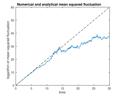
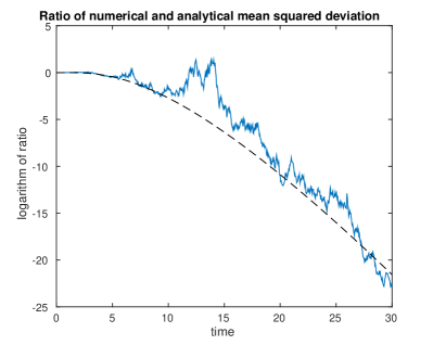
Consequently, any implementation of the Monte Carlo method excluding large deviations will underestimate the true value of 𝔼[v2(t)]𝔼delimited-[]superscript𝑣2𝑡\mathbb{E}[v^{2}(t)] by an exponentially growing factor in time. Let us note that this is also true for any moment of v𝑣v and with general parameters λ𝜆\lambda and σ𝜎\sigma. We illustrate this fact using a numerical simulation. We perform a Monte Carlo simulation in Matlab with 106superscript10610^{6} paths of the process (32)32(\ref{xi}) on the time interval [0,T]0𝑇[0,T] with T=30𝑇30T=30 and 103superscript10310^{3} equidistant sampling points. We impose the initial condition z(0)=0𝑧00z(0)=0 and the parameter values λ=0.5𝜆0.5\lambda=0.5 and σ=1𝜎1\sigma=1. Consequently, z(t)𝑧𝑡z(t) is the Wiener process Btsuperscript𝐵𝑡B^{t}, and for its numerical approximation z¯¯𝑧\bar{z} we use the built-in Matlab procedure normrnd that generates normally distributed random numbers. We calculate v¯(t):=exp(z¯(t))assign¯𝑣𝑡¯𝑧𝑡\bar{v}(t):=\exp(\bar{z}(t)) and evaluate the mean squared fluctuations 𝔼[v¯2(t)]𝔼delimited-[]superscript¯𝑣2𝑡\mathbb{E}[\bar{v}^{2}(t)]. We plot its logarithm as the solid curve in Figure 1(a), compared to the analytical curve log(𝔼[v2(t)])=4λt𝔼delimited-[]superscript𝑣2𝑡4𝜆𝑡\log(\mathbb{E}[v^{2}(t)])=4\,\lambda\,t (dashed line). We observe the exponential in time divergence of the two curves. This is well described by our formula (35), as illustrated in Figure 1(b). For the calculation of the cut-off parameter η𝜂\eta we use the maximal value attained by the actual numerical realization of the stochastic process, i.e., we set η:=maxt(0,T]|z¯(t)|4λtassign𝜂subscript𝑡0𝑇¯𝑧𝑡4𝜆𝑡\eta:=\max_{t\in(0,T]}\frac{|\bar{z}(t)|}{\sqrt{4\,\lambda\,t}}. We then plot the logarithm of the ratio 𝔼[v¯2(t)]/𝔼[v2(t)]𝔼delimited-[]superscript¯𝑣2𝑡𝔼delimited-[]superscript𝑣2𝑡\mathbb{E}[\bar{v}^{2}(t)]/\mathbb{E}[v^{2}(t)] and the theoretically calculated curve given by the right-hand side of (35). We observe a good match between the two curves.
   Refer to caption    Refer to caption

  (a)                                                      (b)

Figure 1: (a) Logarithm of the simulated mean squared fluctuations log(𝔼[v¯2(t)])𝔼delimited-[]superscript¯𝑣2𝑡\log(\mathbb{E}[\bar{v}^{2}(t)]) (solid line), and the analytical result log(𝔼[v2(t)])=4λt𝔼delimited-[]superscript𝑣2𝑡4𝜆𝑡\log(\mathbb{E}[v^{2}(t)])=4\,\lambda\,t (dashed line). (b) Logarithm of the ratio of simulated and analytically calculated mean squared fluctuations 𝔼[v¯2(t)]/𝔼[v2(t)]𝔼delimited-[]superscript¯𝑣2𝑡𝔼delimited-[]superscript𝑣2𝑡\mathbb{E}[\bar{v}^{2}(t)]/\mathbb{E}[v^{2}(t)] (solid line), and the theoretically calculated curve (dashed line) given by the right-hand side of (35)35(\ref{ratio}). The Monte-Carlo simulation for z(t)𝑧𝑡z(t) was performed with 106superscript10610^{6} paths of the process (32)32(\ref{xi}) with z(0)=0𝑧00z(0)=0, λ=0.5𝜆0.5\lambda=0.5 and σ=1𝜎1\sigma=1 on the time interval [0,30]030[0,30] divided into 103superscript10310^{3} equidistant sampling points.

This systematic discrepancy between the analytical formulas and Monte Carlo simulations originates in the heavy tailed distribution of the geometric Brownian motion, and is a well studied topic, see, e.g., the survey [16]. Importance sampling and rare-event simulation techniques would be the methods of choice to overcome this problem, however, their implementation is beyond the scope of our paper. Instead, we argue that the motivation for studying the stochastic system (1)–(2) and its simplification (10) comes from the fact that they ought to represent models of some real (physical or biological) phenomena. In real life situations these extreme events with exponentially low probabilities can be unphysical and the presented Monte Carlo simulation can be considered a more appropriate description of reality than the SDEs. We adopt this point of view for the forthcoming numerical studies in Sections 4.24.3 and 4.4, and accept the fact their results may not be directly related to statements of Theorem 2 and Lemma 4.

4.2 Numerical study of delayed geometric Brownian motion

Using λ=1𝜆1\lambda=1, the delayed SDE (10)10(\ref{simplified}) can be equivalently written as

dw=w~dt+σw~dBt,d𝑤~𝑤d𝑡𝜎~𝑤dsuperscript𝐵𝑡\,\mathrm{d}w=-\widetilde{w}\,\,\mathrm{d}t+\sigma\,\widetilde{w}\,\,\mathrm{d}B^{t}, (36)

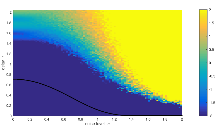
where σ0𝜎0\sigma\geq 0 and τ0𝜏0\tau\geq 0 are nonnegative parameters. We perform a systematic numerical study of the delayed SDE (36)36(\ref{simplified2}) to characterize the asymptotic behaviour of its solutions in dependence on the values of the parameters σ𝜎\sigma and τ𝜏\tau. In particular, we divide the domain [0,2]×[0,2]0202[0,2]\times[0,2] for (σ,τ)𝜎𝜏(\sigma,\tau) into 100×100100100100\times 100 equidistant (σ,τ)𝜎𝜏(\sigma,\tau)-pairs. For each pair of the parameter values we perform a Monte Carlo simulation for (36)36(\ref{simplified2}) with Q=100𝑄100Q=100 paths over the time interval [0,T]0𝑇[0,T] with T=30𝑇30T=30 and timestep Δt=103Δ𝑡superscript103\Delta t=10^{-3}. We impose the constant deterministic initial condition w(t)1𝑤𝑡1w(t)\equiv 1 for t(τ,0]𝑡𝜏0t\in(-\tau,0]. For discretization of (36)36(\ref{simplified2}) we use the Euler-Maruyama method, i.e., the discrete scheme is

wtk+1=wtkΔtwtkτ+σΔt𝒩0,1,k=1,2,,K,formulae-sequencesubscript𝑤subscript𝑡𝑘1subscript𝑤subscript𝑡𝑘Δ𝑡subscript𝑤subscript𝑡𝑘𝜏𝜎Δ𝑡subscript𝒩01𝑘12𝐾\displaystyle w_{t_{k+1}}=w_{t_{k}}-\Delta t\,w_{t_{k}-\tau}+\sigma\,\sqrt{\Delta t}\,\mathcal{N}_{0,1},\qquad k=1,2,\dots,K, (37)

subject to the initial condition wt1subscript𝑤𝑡1w_{t}\equiv 1 for t0𝑡0t\leq 0. Here K=T/Δt𝐾𝑇Δ𝑡K=T/\Delta t denotes the total number of timesteps, tk=kΔtsubscript𝑡𝑘𝑘Δ𝑡t_{k}=k\Delta t, and 𝒩0,1subscript𝒩01\mathcal{N}_{0,1} a normally distributed random variable with zero mean and unit variance. Note that the values of τ𝜏\tau are chosen to be integer multiples of ΔtΔ𝑡\Delta t, so that tkτ=tlsubscript𝑡𝑘𝜏subscript𝑡𝑙t_{k}-\tau=t_{l} for some l𝑙l\in\mathbb{Z}. For each (σ,τ)𝜎𝜏(\sigma,\tau)-pair and each path q𝑞q of the Monte Carlo simulation we calculate the “indicator”

Iσ,τ:=1Qq=1Q(Δtk=(T1)/ΔtT/Δt|wtkq|2)1/2,assignsubscript𝐼𝜎𝜏1𝑄superscriptsubscript𝑞1𝑄superscriptΔ𝑡superscriptsubscript𝑘𝑇1Δ𝑡𝑇Δ𝑡superscriptsubscriptsuperscript𝑤𝑞subscript𝑡𝑘212\displaystyle I_{\sigma,\tau}:=\frac{1}{Q}\sum_{q=1}^{Q}\left(\Delta t\sum_{k=(T-1)/\Delta t}^{T/\Delta t}|w^{q}_{t_{k}}|^{2}\right)^{1/2},

where wtqsubscriptsuperscript𝑤𝑞𝑡w^{q}_{t} is the q𝑞q-th path in the Monte Carlo simulation of (37)37(\ref{discrete}). The background colour in Figure 2 encodes the logarithm of Iσ,τsubscript𝐼𝜎𝜏I_{\sigma,\tau}. To define a region of “numerical convergence”, we choose a threshold ΘΘ\Theta such that I0,τc=Θsubscript𝐼0subscript𝜏𝑐ΘI_{0,\tau_{c}}=\Theta for the delay τc=π2subscript𝜏𝑐𝜋2\tau_{c}=\frac{\pi}{2} that is critical for the problem without noise (σ=0𝜎0\sigma=0). In our case this led to Θ102similar-to-or-equalsΘsuperscript102\Theta\simeq 10^{-2}. The region of “numerical convergence” is marked dark blue in Figure 2. We observe the decrease of the critical value of the delay with increasing level of noise. For comparison, the critical values of τ𝜏\tau given by formula (31)31(\ref{condDGBM}) as a function of σ𝜎\sigma are indicated by the solid line.

Refer to caption


Figure 2: Results of Monte Carlo simulations of the delayed SDE (36)36(\ref{simplified2}) with Q=100𝑄100Q=100 paths for (σ,τ)[0,2]×[0,2]𝜎𝜏0202(\sigma,\tau)\in[0,2]\times[0,2]. The background colour encodes log(Iσ,τ)subscript𝐼𝜎𝜏\log(I_{\sigma,\tau}). The region of “numerical convergence” is dark blue. The solid line indicates the critical values of τ𝜏\tau given by formula (31)31(\ref{condDGBM}) with λ=1𝜆1\lambda=1 as a function of σ𝜎\sigma.

4.3 Numerical study of the system (8)8(\ref{CS0}) with fixed communication matrix

We present results of numerical simulations of the system (8)8(\ref{CS0}) in the one-dimensional setting d=1𝑑1d=1, where we fix the communication rates to ψij1subscript𝜓𝑖𝑗1\psi_{ij}\equiv 1 for all i,j=1,2,,Nformulae-sequence𝑖𝑗12𝑁i,j=1,2,\dots,N, i.e., every agent communicates with all others at the same rate. Consequently, the communication matrix 𝔸𝔸\mathbb{A} has the off-diagonal entries 𝔸ij=1subscript𝔸𝑖𝑗1\mathbb{A}_{ij}=-1, ij𝑖𝑗i\neq j, and 𝔸ii=N1subscript𝔸𝑖𝑖𝑁1\mathbb{A}_{ii}=N-1. It only has two eigenvalues, 00 and N𝑁N. Consequently, its Fiedler number is μ2=Nsubscript𝜇2𝑁\mu_{2}=N and we can choose :=Nassign𝑁\ell:=N in (13)13(\ref{fiedlervect}). In this setting, we can directly compare our analytical result, Theorem 2, with numerical simulations.

We will be considering even number of agents N=2K𝑁2𝐾N=2K, in particular, N{2,20}𝑁220N\in\{2,20\}, and prescribe the initial datum

vi(t){1for i=1,2,,K;1for i=K+1,K+2,,N;\displaystyle v_{i}(t)\equiv\left\{\begin{matrix}-1&\quad\mbox{for }i=1,2,\dots,K;\hfill\\ 1&\quad\mbox{for }i=K+1,K+2,\dots,N;\end{matrix}\right. (38)

for t(τ,0]𝑡𝜏0t\in(-\tau,0]. Although the asymptotic behaviour of the solutions in general depends on the particular choice of the initial datum, a systematic study of this dependence is beyond the scope of this paper. Therefore we only consider the “generic” choice of initial conditions (38).

We perform Monte Carlo simulations of the system (8)8(\ref{CS0}) with N{2,20}𝑁220N\in\{2,20\}, σi=σsubscript𝜎𝑖𝜎\sigma_{i}=\sigma for all i=1,2,,N𝑖12𝑁i=1,2,\dots,N and λ=1𝜆1\lambda=1 (other values of λ𝜆\lambda can be achieved by rescaling of σ𝜎\sigma and time). We divide the domain [0,2]×[0,2]0202[0,2]\times[0,2] for (σ,τ)𝜎𝜏(\sigma,\tau) into 50×50505050\times 50 equidistant (σ,τ)𝜎𝜏(\sigma,\tau)-pairs. For each pair of the parameter values we perform a Monte Carlo simulation with Q=100𝑄100Q=100 paths over the time interval [0,T]0𝑇[0,T] with T=30𝑇30T=30. We use the Euler-Maruyama method for discretization of (8)8(\ref{CS0}) with timestep Δt=103Δ𝑡superscript103\Delta t=10^{-3}. To classify the asymptotic behaviour of the solution, we again define the “indicator”

Iσ,τ:=1Qq=1Q(ΔtNk=(T1)/ΔtT/Δt|𝐯tkq|2)1/2assignsubscript𝐼𝜎𝜏1𝑄superscriptsubscript𝑞1𝑄superscriptΔ𝑡𝑁superscriptsubscript𝑘𝑇1Δ𝑡𝑇Δ𝑡superscriptsubscriptsuperscript𝐯𝑞subscript𝑡𝑘212\displaystyle I_{\sigma,\tau}:=\frac{1}{Q}\sum_{q=1}^{Q}\left(\frac{\Delta t}{N}\sum_{k=(T-1)/\Delta t}^{T/\Delta t}|\mathbf{v}^{q}_{t_{k}}|^{2}\right)^{1/2} (39)

where 𝐯tkqsubscriptsuperscript𝐯𝑞subscript𝑡𝑘\mathbf{v}^{q}_{t_{k}} is the q𝑞q-th path in the Monte Carlo simulation of (1)1(\ref{CS01})(2)2(\ref{CS02}) at time tk=kΔtsubscript𝑡𝑘𝑘Δ𝑡t_{k}=k\Delta t. We say that numerical flocking takes place when Iσ,τ<102subscript𝐼𝜎𝜏superscript102I_{\sigma,\tau}<10^{-2}. The background colour in Figure 3 encodes the decadic logarithm of the indicator, and the dark blue region indicates numerical flocking. We observe that the region of numerical flocking is only weakly influenced by the number of agents N𝑁N. This is in agreement with the fact that the flocking condition (17)17(\ref{flockingCond}) in Theorem 2 does not depend on N𝑁N. The increased smoothness of the colour transition when N=20𝑁20N=20 is a consequence of the law of large numbers. For comparison, the critical value τcsubscript𝜏𝑐\tau_{c} given by formula (17)17(\ref{flockingCond}) for λ=1𝜆1\lambda=1 as a function of σ𝜎\sigma is indicated by the solid line in both panels. The comparison with the numerical results suggests that the condition (17)17(\ref{flockingCond}) is far from optimal.

   Refer to caption    Refer to caption

  (a) N=2𝑁2N=2                                             (b) N=20𝑁20N=20

Refer to caption

Figure 3: Decadic logarithm of the indicator Iσ,τsubscript𝐼𝜎𝜏I_{\sigma,\tau}, given by (39)39(\ref{indicator}), for Monte Carlo simulations of the system (8)8(\ref{CS0}) with Q=100𝑄100Q=100 paths on the time interval [0,30]030[0,30] subject to the initial condition (38)38(\ref{ICv}), with λ=1𝜆1\lambda=1, (σ,τ)[0,2]×[0,2]𝜎𝜏0202(\sigma,\tau)\in[0,2]\times[0,2]. The dark blue regions (colour online) indicate “numerical flocking”. The solid line indicates the critical value τcsubscript𝜏𝑐\tau_{c} given by formula (17)17(\ref{flockingCond}) for λ=1𝜆1\lambda=1 as a function of σ𝜎\sigma. The number of individuals is: (a) N=2𝑁2N=2; and (b) N=20𝑁20N=20.

4.4 Numerical study of the delayed Cucker-Smale system with multiplicative noise

Finally, we present results of numerical simulations of the system (1)1(\ref{CS01})(2)2(\ref{CS02}) in the one-dimensional setting d=1𝑑1d=1 with the communication rates ψij=ψ(|xixj|)subscript𝜓𝑖𝑗𝜓subscript𝑥𝑖subscript𝑥𝑗\psi_{ij}=\psi(|x_{i}-x_{j}|) and ψ𝜓\psi given by (5)5(\ref{commRate}). As in Section 4.3, our goal is to characterize the asymptotic behaviour of the solutions in dependence on the parameter values, however, we are facing additional difficulties here. In particular, the asymptotic behaviour of the solution may depend nontrivially on the initial condition, as we show in Figure 4. Since a systematic study taking this effect into account is beyond the scope of this paper, we will impose the same type of initial condition for all our simulations. In particular, we prescribe constant zero value for the 𝐱𝐱\mathbf{x}-variables,

xi(t)0for t(τ,0],i=1,2,,N.formulae-sequencesubscript𝑥𝑖𝑡0formulae-sequencefor 𝑡𝜏0𝑖12𝑁\displaystyle x_{i}(t)\equiv 0\quad\mbox{for }t\in(-\tau,0],\;i=1,2,\dots,N. (40)

For the 𝐯𝐯\mathbf{v}-variables we impose again the initial datum (38)38(\ref{ICv}).

Refer to caption

  (a)                                                      (b)

Figure 4: Numerical simulations of the system (1)1(\ref{CS01})(2)2(\ref{CS02}), (5)5(\ref{commRate}) with parameter values N=2𝑁2N=2, λ=1𝜆1\lambda=1, β=0.1𝛽0.1\beta=0.1, σ=0𝜎0\sigma=0 and τ=1.75𝜏1.75\tau=1.75. Both simulations are performed on the time interval [0,120]0120[0,120] with discrete timestep Δt=103Δ𝑡superscript103\Delta t=10^{-3}. The initial condition for v𝑣v is v1(t)1subscript𝑣1𝑡1v_{1}(t)\equiv 1, v2(t)1subscript𝑣2𝑡1v_{2}(t)\equiv-1 for t(τ,0]𝑡𝜏0t\in(-\tau,0] in both cases. The initial condition for x𝑥x is: (a) x1(t)1subscript𝑥1𝑡1x_{1}(t)\equiv-1, x2(t)1subscript𝑥2𝑡1x_{2}(t)\equiv 1; (b) x1(t)1subscript𝑥1𝑡1x_{1}(t)\equiv 1, x2(t)1subscript𝑥2𝑡1x_{2}(t)\equiv-1. The plots show the velocities of the two agents (red and blue, colour online) as functions of time.

We perform Monte Carlo simulations of the system (1)1(\ref{CS01})(2)2(\ref{CS02}), (5)5(\ref{commRate}) with N{2,20}𝑁220N\in\{2,20\} and β=0.1𝛽0.1\beta=0.1 (strong coupling) and β=1𝛽1\beta=1 (weak coupling). As in Section 4.3, we fix λ=1𝜆1\lambda=1 and divide the domain [0,2]×[0,2]0202[0,2]\times[0,2] for (σ,τ)𝜎𝜏(\sigma,\tau) into 50×50505050\times 50 equidistant (σ,τ)𝜎𝜏(\sigma,\tau)-pairs. For each pair of the parameter values we perform a Monte Carlo simulation with Q=100𝑄100Q=100 paths over the time interval [0,T]0𝑇[0,T] with T=30𝑇30T=30. We use the Euler-Maruyama method for discretization of (1)1(\ref{CS01})(2)2(\ref{CS02}) with timestep Δt=103Δ𝑡superscript103\Delta t=10^{-3}. To classify the asymptotic behaviour of the solution, we again use the indicator (39)39(\ref{indicator}) and say that numerical flocking takes place when Iσ,τ<102subscript𝐼𝜎𝜏superscript102I_{\sigma,\tau}<10^{-2}. The background colour in Figure 5 encodes the decadic logarithm of the indicator, and the dark blue region indicates numerical flocking.

In the top left panel we indicate by an arrow the point (σ,τ)=(0,1.75)𝜎𝜏01.75(\sigma,\tau)=(0,1.75) that corresponds to the parameter setting in Figure 4; however, note that the initial conditions for xisubscript𝑥𝑖x_{i} in Figure 4 differ from (40)40(\ref{ICx}). We see that the indicated point lies close to the boundary of the dark blue region, i.e., in the “transition zone” between numerical flocking and non-flocking. We hypothesize that this is why we were able to observe the two qualitatively different kinds of asymptotic behaviour in Figure 4 even if the initial datum for the 𝐯𝐯\mathbf{v}-variables is the same in both cases. Again, a systematic study of this hypothesis is beyond the scope of this paper.
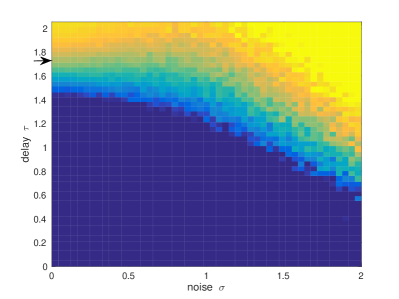
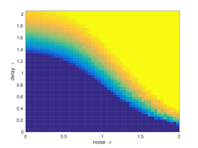
   Refer to caption    Refer to caption

  (a) β=0.1𝛽0.1\beta=0.1, N=2𝑁2N=2                                 (b) β=0.1𝛽0.1\beta=0.1, N=20𝑁20N=20

   Refer to caption    Refer to caption

  (c) β=1𝛽1\beta=1, N=2𝑁2N=2                                    (d) β=1𝛽1\beta=1, N=20𝑁20N=20

Refer to caption

Figure 5: Decadic logarithm of the indicator Iσ,τsubscript𝐼𝜎𝜏I_{\sigma,\tau}, given by (39)39(\ref{indicator}), for Monte Carlo simulations of the system (1)1(\ref{CS01})(2)2(\ref{CS02}), (5)5(\ref{commRate}) with Q=100𝑄100Q=100 paths on the time interval [0,30]030[0,30] subject to the initial conditions (38)38(\ref{ICv}) and (40)40(\ref{ICx}), with λ=1𝜆1\lambda=1 and (σ,τ)[0,2]×[0,2]𝜎𝜏0202(\sigma,\tau)\in[0,2]\times[0,2]. The dark blue regions (colour online) indicate numerical flocking. The arrow in the top left panel indicates the point (σ,τ)=(0,1.75)𝜎𝜏01.75(\sigma,\tau)=(0,1.75) that corresponds to the parameter setting in Figure 4. We use: (a) β=0.1𝛽0.1\beta=0.1, N=2𝑁2N=2; (b) β=0.1𝛽0.1\beta=0.1, N=20𝑁20N=20; (c) β=1𝛽1\beta=1, N=2𝑁2N=2; and (d) β=1𝛽1\beta=1, N=20𝑁20N=20.

In Figure 5 we observe that the region of numerical flocking is only weakly influenced by the number of agents N𝑁N. This is in agreement with the fact that the flocking condition (17)17(\ref{flockingCond}) in Theorem 2 does not depend on N𝑁N. The increased smoothness of the colour transition when N=20𝑁20N=20 is a consequence of the law of large numbers. On the other hand, we can distinguish two distinct types of patterns, one similar to Figure 2 for the strong coupling case β=0.1𝛽0.1\beta=0.1 (Figures 5(a) and 5(b)), and a semicircular pattern for the weak coupling case β=1𝛽1\beta=1 (Figures 5(c) and 5(d)). In particular, the result for the weak coupling case is somewhat surprising – it suggests that for low levels of noise (σ0.6less-than-or-similar-to𝜎0.6\sigma\lesssim 0.6), introduction of intermediate delays (0.3τ1.8less-than-or-similar-to0.3𝜏less-than-or-similar-to1.80.3\lesssim\tau\lesssim 1.8) may facilitate flocking. This is further supported by Figure 6 where we plot sample solutions of (1)1(\ref{CS01})(2)2(\ref{CS02}), (5)5(\ref{commRate}) for N=2𝑁2N=2, β=1𝛽1\beta=1, σ=0𝜎0\sigma=0 (Figure 6(a)), σ=0.5𝜎0.5\sigma=0.5 (Figure 6(b)) and three different values of the delay τ{0,1,2}𝜏012\tau\in\{0,1,2\}. We observe that while for τ=0𝜏0\tau=0 and τ=2𝜏2\tau=2 the agents do not show tendency to converge to a common velocity during the indicated time interval, they exhibit numerical flocking for the intermediate value τ=1𝜏1\tau=1. We will call this observation time-delay induced flocking.

Let us note that the results presented in Figure 6 do not contradict our analytical results. In particular, condition (17)17(\ref{flockingCond}) gives τ<2/40.35𝜏24approaches-limit0.35\tau<\sqrt{2}/4\doteq 0.35 if σ=0𝜎0\sigma=0 and τ<(1/2+11/8)/40.17𝜏121184approaches-limit0.17\tau<(-1/2+\sqrt{11/8})/4\doteq 0.17 if σ=0.5𝜎0.5\sigma=0.5, so it is only satisfied for the simulations in the panels corresponding to τ=0𝜏0\tau=0 in Figure 6. Therefore, statement of Lemma 3 applies. The (expectation of) the Lyapunov function (3.2)3.2(\ref{Lyapunov}) decreases in time for these two simulations.
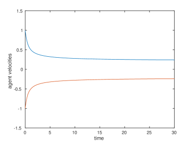
   Refer to caption    Refer to caption

  (a) σ=0𝜎0\sigma=0                                             (b) σ=0.5𝜎0.5\sigma=0.5

τ=0𝜏0\tau=0, σ=0𝜎0\sigma=0                                         τ=0𝜏0\tau=0, σ=0.5𝜎0.5\sigma=0.5

   Refer to caption    Refer to caption

τ=1𝜏1\tau=1, σ=0𝜎0\sigma=0                                         τ=1𝜏1\tau=1, σ=0.5𝜎0.5\sigma=0.5

   Refer to caption    Refer to caption

τ=2𝜏2\tau=2, σ=0𝜎0\sigma=0                                         τ=2𝜏2\tau=2, σ=0.5𝜎0.5\sigma=0.5

Figure 6: Agents velocities v1(t),v2(t)subscript𝑣1𝑡subscript𝑣2𝑡v_{1}(t),v_{2}(t) in sample solutions of the system (1)1(\ref{CS01})(2)2(\ref{CS02}), (5)5(\ref{commRate}) with N=2𝑁2N=2, λ=1𝜆1\lambda=1, β=1𝛽1\beta=1 (weak coupling), on the time interval [0,30]030[0,30] subject to the initial conditions (38)38(\ref{ICv}) and (40)40(\ref{ICx}). We use: (a) σ=0𝜎0\sigma=0; and (b) σ=0.5𝜎0.5\sigma=0.5.

To gain a further understanding of the interesting phenomenon of time-delay induced flocking, we run systematic simulations of the system (1)1(\ref{CS01})(2)2(\ref{CS02}), (5)5(\ref{commRate}) with different values of β[0.5,2.5]𝛽0.52.5\beta\in[0.5,2.5], τ[0,2]𝜏02\tau\in[0,2] and σ{0,0.5}𝜎00.5\sigma\in\{0,0.5\}. We calculate the indicator Iβ,τsubscript𝐼𝛽𝜏I_{\beta,\tau} as in (39)39(\ref{indicator}) with Q=1𝑄1Q=1 for σ=0𝜎0\sigma=0 (there is no need to run more than one path for the case without noise) and Q=100𝑄100Q=100 Monte Carlo paths for σ=0.5𝜎0.5\sigma=0.5. The decadic logarithm of Iβ,τsubscript𝐼𝛽𝜏I_{\beta,\tau} is plotted in Figure 7 and we again use the threshold Iβ,τ<102subscript𝐼𝛽𝜏superscript102I_{\beta,\tau}<10^{-2} to define numerical flocking (dark blue regions in Figure 7). We observe that there exists (for β𝛽\beta sufficiently large) a region of intermediate values of τ𝜏\tau where numerical flocking takes place, while it does not for smaller or larger τ𝜏\tau values. Moreover, we see that noise has a disruptive influence on flocking (the dark blue region is smaller in Figure 7(b) compared to Figure 7(a)).
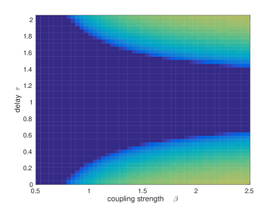
   Refer to caption    Refer to caption

  (a) σ=0𝜎0\sigma=0                                             (b) σ=0.5𝜎0.5\sigma=0.5

Refer to caption

Figure 7: Decadic logarithm of the indicator Iβ,τsubscript𝐼𝛽𝜏I_{\beta,\tau} for simulations of the system (1)1(\ref{CS01})(2)2(\ref{CS02}), (5)5(\ref{commRate}) on the time interval [0,30]030[0,30] with λ=1𝜆1\lambda=1, N=2𝑁2N=2, (β,τ)[0.5,2.5]×[0,2]𝛽𝜏0.52.502(\beta,\tau)\in[0.5,2.5]\times[0,2]. We use: (a) σ=0𝜎0\sigma=0, Q=1𝑄1Q=1; and (b) σ=0.5𝜎0.5\sigma=0.5, Q=100𝑄100Q=100. The dark blue regions (colour online) indicate numerical flocking.

5 Discussion

We have studied a generalization of the Cucker-Smale model accounting for measurement errors through introduction of multiplicative white noise, and for delays in information processing. This has led to a system of stochastic delayed differential equations (1)1(\ref{CS01})(2)2(\ref{CS02}). In Section 3, we have considered the communication rates between agents as given stochastic processes, and derived a sufficient condition for flocking, which we define as asymptotic convergence of the agents’ velocities towards a common value. The condition is given in terms of the critical delay that guarantees flocking as a function of the noise level. Our analysis is based on a construction of a suitable Lyapunov function for the system and a study of its decay. As a byproduct of the analysis, we obtain a sufficient condition for asymptotic convergence of delayed geometric Brownian motion.

The second part of the paper is devoted to systematic numerical simulations. First, we perform Monte Carlo simulations of delayed geometric Brownian motion and evaluate its asymptotic behaviour based on a suitable “numerical indicator”. This led to the conclusion that the analytically derived sufficient condition for asymptotic convergence is qualitatively right - the convergence deteriorates with increasing noise level and delay. However, quantitatively it is far from optimal. Next, we simulate the Cucker-Smale type system with fixed communication rates and again compare with the analytical result. As before, the comparison shows that, while qualitatively correct, the analytical formula produces too restrictive critical delays. Finally, we simulate the full Cucker-Smale system with delays and multiplicative noise. We use two regimes for the dependence of the communication rates on the agents’ distances: the strong coupling regime, which leads to unconditional flocking in the “classical” Cucker-Smale model, and the weak coupling regime, where flocking may or may not take place. In the strong coupling regime the numerical picture is similar to the previous simulation with fixed communication rates. On the other hand, in the weak coupling regime we observe a somehow surprising behaviour of the system - namely, that an introduction of intermediate time delay may facilitate flocking. We call this phenomenon “delay induced flocking”.

Our paper leaves several open questions. First of all, our analytical flocking condition is too restrictive compared to numerical results, so efforts should be made to improve it. Moreover, the analysis applied to the case when the communication rates are given and satisfying a certain structural assumption. This is in fact against the spirit of the original Cucker-Smale model where the communication rates depend on the mutual distances between agents. A possible extension of our analysis to this case remains an open problem. The main difficulty is due to the fact that it is not clear how to apply the classical bootstrapping argument that bounds the velocity fluctuations in terms of fluctuations in positions and vice versa. For the numerical part, it would be desirable to apply some multilevel Monte Carlo or importance sampling technique to obtain more accurate results. Moreover, the influence of the initial condition on the asymptotic behaviour should be studied. Finally, the interesting phenomenon of “delay induced flocking” deserves a detailed study, both from the analytical and numerical point of view.

References

  • [1] S. Ahn, and S.-Y. Ha, Stochastic flocking dynamics of the Cucker- Smale model with multiplicative white noises, Journal of Mathematical Physics 51, 2010, pp. 103301.
  • [2] A. Amman, E. Schöll, and W. Just, Some basic remarks on eigenmode expansions of time-delay dynamics, Physica A 373, 2007.
  • [3] J. Appleby, X. Mao, and M. Riedle, Geometric Brownian motion with delay: mean square characterisation, Proceedings of The American Mathematical Society 137 (1), 2009, pp. 339–348.
  • [4] J. Carrillo, M. Fornasier, J. Rosado, and G. Toscani, Asymptotic Flocking Dynamics for the kinetic Cucker-Smale model, SIAM Journal on Mathematical Analysis 42 (1), 2010, pp. 218–236.
  • [5] J. Carrillo, M. Fornasier, G. Toscani, and F. Vecil, Particle, kinetic, and hydrodynamic models of swarming, In Naldi, G., Pareschi, L., Toscani, G. (eds.), Mathematical Modeling of Collective behaviour in Socio-Economic and Life Sciences, Series: Modelling and Simulation in Science and Technology, Birkhäuser, 2010, pp. 297–336.
  • [6] F. Cucker, and S. Smale, Emergent behaviour in flocks, IEEE Transactions on Automatic Control 52, 2007, pp 852–862.
  • [7] F. Cucker, and S. Smale, On the mathematics of emergence, Japanese Journal of Mathematics 2, 2007, pp. 197–227.
  • [8] L. El’sgol’ts, and S. Norkin, translated by J. Casti, Introduction to the theory and application of differential equations with deviating arguments, Academic Press, New York, 1973.
  • [9] R. Erban, From molecular dynamics to Brownian dynamics, Proceedings of the Royal Society A 470, 2014, 20140036.
  • [10] R. Erban and J. Haskovec, From individual to collective behaviour of coupled velocity jump processes: a locust example, Kinetic and Related Models 5(4), 2012, pp. 817-842
  • [11] B. Franz, J. Taylor-King, C. Yates and R. Erban, Hard-sphere interactions in velocity jump models, submitted to Physical Review E, available as http://arxiv.org/abs/1409.7959 (2014)
  • [12] S. Gillouzic, Fokker-Planck approach to stochastic delay differential equations, Thesis, Ottawa, Canada, 2000.
  • [13] S.-Y. Ha, K. Lee, and D. Levy, Emergence of time-asymptotic flocking in a stochastic Cucker-Smale system, Communication in Mathematical Sciences 7, 2009, pp. 453–469.
  • [14] S.-Y. Ha, and J.-G. Liu, A simple proof of the Cucker-Smale flocking dynamics and mean-field limit, Communication in Mathematical Sciences 7, 2009, pp. 297–325.
  • [15] J. Haskovec, Flocking dynamics and mean-field limit in the Cucker-Smale-type model with topological interactions, Physica D - Nonlinear Phenomena 261, 2013, pp. 42–51.
  • [16] S. Juneja, and P. Shahabuddin, Rare-event Simulation Techniques: An Introduction and Recent Advances, In: Shane G. Henderson and Barry L. Nelson, Editor(s), Handbooks in Operations Research and Management Science, Elsevier, Vol. 13, 2006, pp. 291–350.
  • [17] V. Kolmanovskii, and A. Myshkis, Applied theory of functional differential equations, Kluwer, Boston, 1992.
  • [18] Y. Liu, and J. Wu, Flocking and asymptotic velocity of the Cucker-Smale model with processing delay, Journal of Mathematical Analysis and Applications 415, 2014, pp. 53–61.
  • [19] X. Mao, Stochastic Differential Equations and Applications, Second Edition, Horwood Publishing Limited, 2007.
  • [20] X. Mao, Stability and stabilisation of stochastic differential delay equations, IET Control Theory Appl. 1 (6), pp. 1551–1566, 2007.
  • [21] S. Motsch, and E. Tadmor, A new model for self-organized dynamics and its flocking behaviour, Journal of Statistical Physics 144, 2011, pp. 923–947.
  • [22] B. Øksendal, Stochastic Differential Equations, Springer-Verlag Heidelberg New York, 2000.
  • [23] L. Pareschi, and G. Toscani, Interacting Multiagent Systems: Kinetic equations and Monte Carlo methods, Oxford University Press, 2014.
  • [24] J. Peszek, Existence of piecewise weak solutions of a discrete Cucker-Smale’s flocking model with a singular communication weigh, Journal of Differential Equations 257 (8), 2014, pp. 2900–2925.
  • [25] H. Smith, An Introduction to Delay Differential Equations with Applications to the Life Sciences, Springer New York Dordrecht Heidelberg London, 2011.
  • [26] D. Sumpter, Collective Animal Behavior, Princeton University Press, 2010.
  • [27] Y. Sun, W. Lin and R. Erban, Time delay can facilitate coherence in self-driven interacting particle systems, Physical Review E 90(6), 2014, 062708.
  • [28] S.-Y. Ha, and E. Tadmor, From particle to kinetic and hydrodynamic descriptions of flocking, Kinetic and Related models 1, 2008, pp. 315–335.
  • [29] T. Ton, N. Linh, and A. Yagi, Flocking and non-flocking behaviour in a stochastic Cucker-Smale system, Analysis and Applications 12 (1), 2014, pp. 63-73.
  • [30] J. Taylor-King, B. Franz, C. Yates and R. Erban, Mathematical modelling of turning delays in swarm robotics, IMA Journal of Applied Mathematics 2015, doi: 10.1093/imamat/hxv001.
  • [31] T. Vicsek, and A. Zafeiris, Collective motion, Physics Reports, 2012.