Competing Effects of Social Balance and Influence

Abstract

We study a three-state (leftist, rightist, centrist) model that couples the dynamics of social balance with an external deradicalizing field. The mean-field analysis shows that there exists a critical value of the external field $p_{c}$ such that for a weak external field ($p$$<$$p_{c}$), the system exhibits a metastable fixed point and a saddle point in addition to a stable fixed point. However, if the strength of the external field is sufficiently large ($p$$>$$p_{c}$), there is only one (stable) fixed point which corresponds to an all-centrist consensus state (absorbing state). In the weak-field regime, the convergence time to the absorbing state is evaluated using the quasi-stationary distribution and is found to be in agreement with the results obtained by numerical simulations.

I Introduction

Structural balance is considered to be one of the key driving mechanisms of social dynamics Heider ; Wasserman_1994 ; Lambiotte_PNAS2010 and since its introduction by Heider Heider , it has been studied extensively in the context of social networks Lambiotte_PNAS2010 ; Cartwright_1956 ; Antal_PRE ; Antal_Physica ; Marvel_balance . In a socially interacting population, relationships among individuals (links in the underlying social network) can be classified as friendly (+) or unfriendly (-). Evolution of these links is governed by the theory of structural balance, also referred to as social balance. The underlying axioms behind this theory are: (i) a friend of my friend or an enemy of my enemy is my friend, and (ii) a friend of my enemy or an enemy of my friend is my enemy. In the context of social networks, a triangle is said to be unbalanced if it contains an odd number of unfriendly links Antal_PRE ; Antal_Physica . According to the theory of social balance, these unbalanced triangles have a tendency to evolve to balanced configurations Heider ; Cartwright_1956 . This might happen by transitioning nodes and/or interpersonal links in such a way that the conditions of social balance are satisfied. For example, a triad in which two mutually antagonistic individuals have a common friend, is by definition unbalanced but can become balanced by requiring either the common friend to choose a side or the mutually antagonistic two nodes to reconcile their conflict and become friends. A structurally balanced network contains no unbalanced triangles. Here, we construct an individual-based model where the dynamics (in part) is driven by structural balance, but (unlike in previous works Antal_PRE ; Antal_Physica ; Marvel_balance ; Galam96 ; GalamEPJB14 ; Galam_war_peace ) a change in the state of an edge is the direct consequence of a change in the state (opinion) of one of the nodes the edge connects. Another key feature of the model studied here is that triadic (three-body) interactions among nodes have been considered as opposed to dyadic (pair-wise) interactions in three-state models Mobilia2013 ; Vazquez2004 ; Zhang_scirep ).

In this paper, we consider a population where each individual is in one of the three possible opinion states (leftist, rightist, or centrist) Mobilia2013 ; Vazquez2004 ; Zhang_scirep . A link that connects two extremists of opposite type (i. e. the link between a leftist and a rightist) is considered to be unfriendly while all other links are friendly. Thus, a triangle containing one node of each type (leftist, rightist, and centrist) is unbalanced. An unbalanced triangle can be balanced in a number of ways with each minimal change solution requiring one node in the triangle updating its opinion. In a model with extremist and moderate opinion states of individuals, Marvel et al. Marvel_PRL2012 showed that moderation by external stimulus is a way to have a society adopt a moderate viewpoint (non-social deradicalization). Here, in our model, we consider a similar external influence field (e.g., campaigns, advertisements) which converts extremists into centrists. Thus, the system is governed by the competing effects of social balance and influence.

At each time step either with probability $p$ (i) random node is selected and if it is an extremist, it is converted to a centrist, or with the complementary probability $(1-p)$ (ii) a random triangle is selected and if unbalanced, it is balanced by either converting (with a probability $\alpha$) a centrist into an extremist or [with a probability $(1-\alpha)$] an extremist into a centrist. Furthermore, since an extremist can either be a leftist or a rightist, a choice of converted extremist flavor is made with equal probability ($\frac{1}{2}$) as shown in Fig. 1.

Figure 1: The balance step is taken with probability $(1-p)$. However, balance can be achieved in two ways: (a) with probability $\alpha$ a centrist is converted into an extremist and since it can either be a leftist or a rightist, its flavor is chosen randomly with equal probability $1/2$. (b) Alternatively, with probability $(1-\alpha)$ an extremist (either leftist or rightist with equal probability $1/2$) is converted to a centrist.

II Fully-connected networks (Mean-field analysis)

II.1 Fixed points of the system

For a fully-connected network, at any given time the state of a system of size $N$ can be described by two numbers - the density (fraction) of leftists ($x$) and the density of rightists ($y$) - as we can eliminate the density of centrists ($z$) since $x+y+z=1$. Thus, the evolution can be mapped onto the $xy$ plane. A finite system will always have only one absorbing fixed point (for $p>0$) that is a consensus state where every node has adopted the centrist opinion. First, for simplicity, we consider this dynamics on an infinite complete graph where every node is connected to every other node (i.e., in the mean-field limit). Starting from an arbitrary state ($x>0$, $y>0$, $z>0$), in the absence of an external influencing field ($p=0$), the final state of the system is either polarized ($z=0$) or is a coalition where mixed population of centrists and extremists of one kind (either leftist or rightist) coexists. For $p=0$, the whole triangular boundary of the phase space in the $xy$ plane becomes absorbing, thus, a pure consensus state in this case can not be reached through transitions from a different initial state (see Appendix A). For $p>0$, the evolution of $x,y$ densities is governed by the following rate equations:

$$\frac{dx}{dt} = -px+3(2\alpha-1)(1-p)xy(1-x-y)$$ (1)

$$\frac{dy}{dt} = -py+3(2\alpha-1)(1-p)xy(1-x-y)\;.$$ (2)

A trivial solution of these equations is the all-centrist consensus state, i.e., $(x,y)=(0,0)$ (or equivalently $z=1$). However, the steady state solution (see Appendix B) of these equations with $\alpha>\frac{1}{2}$ shows the existence of a critical point,

$$p_{c}=\frac{3(2\alpha-1)}{8+3(2\alpha-1)}\;,$$ (3)

such that for $p<p_{c}$ the system exhibits two non-trivial fixed points as well:

$$(x,y)=\left(\frac{1}{4}+\frac{1}{4}\sqrt{1-\frac{8p}{3(2\alpha-1)(1-p)}}\right)(1,1)\;,$$ (4)

which is a metastable fixed point and

$$(x,y)=\left(\frac{1}{4}-\frac{1}{4}\sqrt{1-\frac{8p}{3(2\alpha-1)(1-p)}}\right)(1,1)\;,$$ (5)

which is a saddle point (unstable fixed point). In the other scenario, when $\alpha<\frac{1}{2}$, the system already has the tendency to move towards an all-centrist consensus state, hence only the trivial fixed point $(x,y)=(0,0)$ exists.

In this paper we focus on the case of $\alpha>\frac{1}{2}$ in which the system has the tendency to become polarized and the external influence field is required to prevent this polarization. In this regime, due to the competition between balancing and influencing forces, the densities fluctuate around the metastable point and the system is trapped for exponentially long times before unlikely large fluctuation moves it to the absorbing state. Here all fixed points lie on the line $y=x$ as shown in Fig. 2 and any asymmetry in $x$ and $y$ decays exponentially fast KornissJSP ; Haken (see Appendix B). The trajectories shown in Fig. 2 are exact only in the thermodynamic limit (fully-connected network in the limit of $N\to\infty$).

Figure 2: (Color online) Phase-space trajectories within mean-field approximation for $\alpha$$=$$0.75$ for which $p_{c}$$\approx$$0.16$, (a) for $p$$=$$0.12$$<$$p_{c}$, and (b) for $p=$$0.20$$>$$p_{c}$.

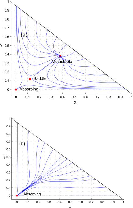
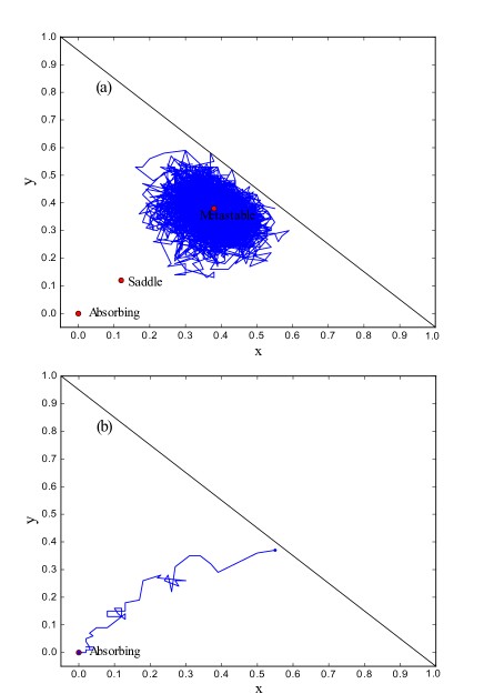
It can be seen explicitly that a finite network ($N=100$) in the weak-field limit ($p<p_{c}$) gets stuck in the metastable state and never crosses the saddle point whereas a fast centrist consensus is reached when $p>p_{c}$ (Fig. 3).

Figure 3: (Color online) Stochastic trajectories for a fully-connected network of size $N=100$ and $\alpha=0.75$, (a) for $p$$=$$0.12$$<$$p_{c}$, and (b) for $p=$$0.20$$>$$p_{c}$. See also Supplemental Material for animations of the above two scenarios (for the same parameters).

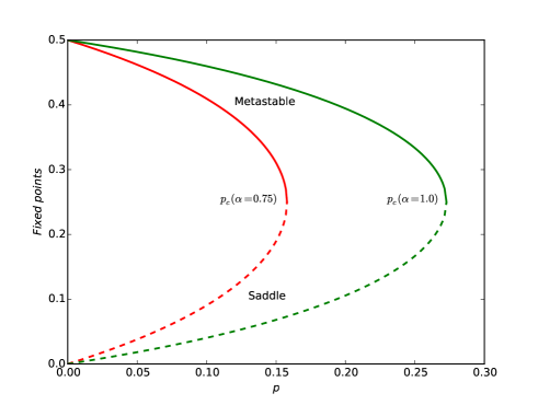
It is also clear from the above that the locations of the fixed points (roots) depend on the choice of $\alpha$ ($>\frac{1}{2}$) and $p$. For a particular choice of $\alpha$, the two fixed points (metastable and saddle) move closer to each other as $p$ is increased from $0$ till they meet and annihilate each other at $p=p_{c}$ (as shown in Fig. 4). Beyond $p_{c}$, these additional fixed points cease to exist and the only fixed point is the consensus state ($x=y=0$).

Figure 4: (Color online) The locations ($x$, $y$ co-ordinates) of metastable (solid lines) and saddle (dashed lines) fixed points for $\alpha=0.75$ (red) and $\alpha=1.0$ (green) obtained from the solution of the rate equations. $x=y$ for all fixed points.

II.2 Consensus time for finite-size networks

An all centrist consensus state is always reached for a finite network. Time to reach this absorbing state (consensus time $T_{c}$) can be obtained by direct simulations. This approach works well for $p>p_{c}$, however, for $p<p_{c}$ (specially when $p<<p_{c}$ and/or $N>>1$), $T_{c}$ becomes so large that its estimation by simulation becomes difficult if at all possible. We therefore use the quasi-stationary (QS) approximation prescribed in Dickman2002 and also used in xie2011 ; Dickman2004 to estimate $T_{c}$ in the region $p<p_{c}$.

We start by introducing notation for the numbers of nodes with the given opinion, thus, $X=xN$, $Y=yN$, and $Z=zN$. Then we form the master equation that describes the time evolution of probability $P_{X,Y}$ (the probability that system has $X$ leftists and $Y$ rightists at time $t$).

$$\frac{1}{N}\frac{dP_{X,Y}}{dt} = {P}_{X-1,Y}\frac{3\alpha(1-p)(X-1)Y(N-X+1-Y)}{N(N-1)(N-2)}$$ (6)

$$+ {P}_{X,Y-1}\frac{3\alpha(1-p)X(Y-1)(N-X-Y+1)}{N(N-1)(N-2)}$$

$$+ {P}_{X+1,Y}\frac{3(1-\alpha)(1-p)(X+1)Y(N-X-1-Y)}{N(N-1)(N-2)}$$

$$+ {P}_{X+1,Y}~{}p~{}\frac{X+1}{N}$$

$$+ {P}_{X,Y+1}\frac{3(1-\alpha)(1-p)X(Y+1)(N-X-Y-1)}{N(N-1)(N-2)}$$

$$+ {P}_{X,Y+1}~{}p~{}\frac{Y+1}{N}$$

$$- P_{X,Y}\frac{6(1-p)XY(N-X-Y)}{N(N-1)(N-2)}$$

$$- P_{X,Y}~{}p~{}\frac{X+Y}{N}\;.$$

Within the triangular region (bounded by $0\leq X\leq(N-Y)$ and $0\leq Y\leq(N-X)$), the transitions allowed from a state ($X$, $Y$) are to states ($X\pm 1$, $Y$) or ($X$, $Y\pm 1$) with the constraint that the system stays within the bounded region. The positive and negative terms on the right side of the master equation contribute to the net flow of probability into and out of the state ($X$,$Y$), respectively. A factor of $\frac{1}{N}$ on the left-hand side appears because a microscopic step of transition from initial state to the final state takes place in a time interval $1/N$. $\frac{6~{}X~{}Y~{}(N-X-Y)}{N(N-1)(N-2)}$ is the density of unbalanced triangles at any given time for a fully-connected network.

The QS distribution of occupation probabilities is given by $\tilde{P}_{X,Y}=P_{X,Y}(t)/P_{S}(t)$ where $P_{S}(t)$ is the survival probability. Under the QS hypothesis, the survival probability decays exponentially, governed by

$$\frac{dP_{S}(t)}{dt}=-P_{S}(t)\tilde{Q}_{0}\;,$$ (7)

where $\tilde{Q}_{0}=p[\tilde{P}_{1,0}+\tilde{P}_{0,1}]$ measures the flow of probability into the absorbing state $(0,0)$. The underlying idea of QS hypothesis is that the occupation probability distribution conditioned on survival (over all $(X,Y)$ except the absorbing state) is stationary. Therefore,

$$\frac{dP_{X,Y}}{dt}=\tilde{P}_{X,Y}\frac{dP_{S}(t)}{dt}\;.$$ (8)

We plug in $P_{X,Y}$ in terms of $\tilde{P}_{X,Y}$ into the master equation to obtain the QS distribution,

$$\tilde{P}_{X,Y}=\frac{\tilde{Q}_{X,Y}}{W_{X,Y}-\tilde{Q}_{0}}\;,$$ (9)

where $W_{X,Y}=\frac{6(1-p)XY(N-X-Y)}{(N-1)(N-2)}+p(X+Y)$, and

$$\tilde{Q}_{X,Y} = \tilde{P}_{X-1,Y}\frac{3\alpha(1-p)(X-1)Y(N-X+1-Y)}{(N-1)(N-2)}$$

$$+ \tilde{P}_{X,Y-1}\frac{3\alpha(1-p)X(Y-1)(N-X-Y+1)}{(N-1)(N-2)}$$

$$+ \tilde{P}_{X+1,Y}\frac{3(1-\alpha)(1-p)(X+1)Y(N-X-1-Y)}{(N-1)(N-2)}$$

$$+ \tilde{P}_{X+1,Y}~{}p~{}(X+1)$$

$$+ \tilde{P}_{X,Y+1}\frac{3(1-\alpha)(1-p)X(Y+1)(N-X-Y-1)}{(N-1)(N-2)}$$

$$+ \tilde{P}_{X,Y+1}~{}p~{}(Y+1)\;.$$

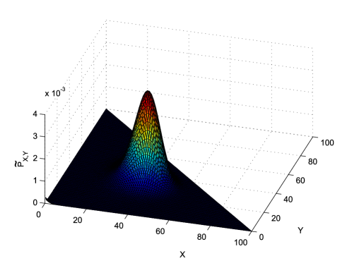
Starting from an arbitrary distribution $\tilde{P}_{X,Y}^{0}$, an asymptotic QS distribution $\tilde{P}_{X,Y}$ can be obtained by the iteration: $\tilde{P}_{X,Y}^{i+1}=a~{}\tilde{P}_{X,Y}^{i}+(1-a)~{}\frac{\tilde{Q}_{X,Y}^{i}}{W_{X,Y}^{i}-\tilde{Q}_{0}^{i}}$, where $0\leq a\leq 1$ is an arbitrary parameter xie2011 . The QS distribution for a particular system size $N=100$ (fully-connected), $p=0.12$, and $\alpha=0.75$ with parameter $a=0.5$ is shown in Fig. 5. In this case a satisfactory convergence was obtained in $40000$ iterations. As expected from the mean-field analysis (for $\alpha=0.75$, the metastable fixed point $(x,y)=(0.38,0.38)$) the distribution peaks around $(X,Y)=(38,38)$.

Figure 5: (Color online) The QS distribution with $a$$=$$0.5$ for $N$$=$$100$, $\alpha$$=$$0.75$, $p$$=$$0.12$. For these parameters, $p_{c}$$\approx$$0.16$.

Once the desired QS distribution is obtained, the mean consensus time $T_{c}$ is computed from the decay rate of the survival probability,

$$T_{c}\simeq\frac{1}{p~{}[\tilde{P}_{1,0}+\tilde{P}_{0,1}]}\;.$$ (10)

Figure 6: (Color online) Consensus time $T_{c}$ obtained from the QS distribution and by direct MC simulations for $\alpha$$=$$0.75$ ($p_{c}$$\approx$$0.16$).

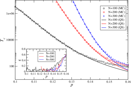
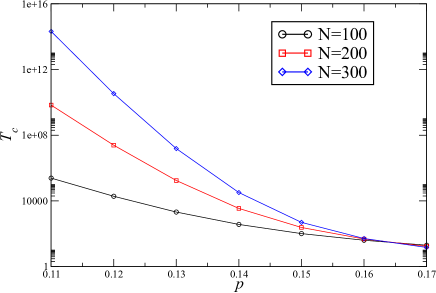
We compare $T_{c}$ obtained from the QS approximation to that obtained by direct Monte Carlo (MC) simulations in the region of $p<p_{c}$ where $T_{c}$ could be easily obtained by both methods for the respective system sizes [Fig. 6]. One can see that there is a good agreement between the two methods across many system sizes and the agreement is getting better as $p$ is decreased below $p_{c}$ as shown in Fig. 6. The change in the relative error with respect to $p$ and $N$, $\epsilon=\frac{\lvert T_{c}(QS)-T_{c}(MC)\rvert}{T_{c}(MC)}$ can be seen in the inset. Figure 7 shows $T_{c}$ obtained by the QS approximation as a function of $p$ for the entire range of $p$ considered for all system sizes, where MC simulations become prohibitive to estimate $T_{c}$. The consensus time $T_{c}$ shows an exponential scaling with $N$ for $p<p_{c}$ as shown in Fig. 8.

Figure 7: (Color online) Consensus time $T_{c}$ computed by the QS approximation as a function of $p$ in the weak-field regime for $\alpha$$=$$0.75$ ($p_{c}$$\approx$$0.16$).

Figure 8: (Color online) Consensus time $T_{c}$ computed by the QS approximation as a function of system size $N$ in the weak-field regime for $\alpha$$=$$0.75$ ($p_{c}$$\approx$$0.16$).

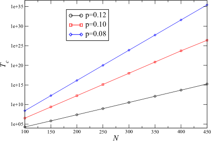
In order to obtain the dependence of $T_{c}$ on $p$, we assume a relation common in systems with tipping points and barrier crossing xie2011 ; xie2012 ,

$$T_{c}=f(N)\exp[\beta(p)N]\;,$$ (11)

where $f(N)$ is increasing slower than exponential with $N$ and

$$\beta(p)\sim\lvert p_{c}-p\rvert^{\nu}\;.$$ (12)

With $T_{c}(p_{c})=f(N)$, we have

$$\ln(T_{c})-\ln(T_{c}(p_{c}))=\beta(p)N\;.$$ (13)

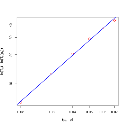
As can be seen from Fig. 9, the growth rate approximately follows the scaling behavior $\beta\sim\lvert p_{c}-p\rvert^{\nu}$ with the measured exponent $\nu\approx 1.57$.

Figure 9: (Color online) $\ln(T_{c})-\ln(T_{c}(p_{c}))$ as a function of $(p_{c}-p)$ on a log-log scale. The exponent $\nu$ is given by the slope of the fitted line ($N=300$, $\alpha=0.75$, $p_{c}$$\approx$$0.16$, $\nu\approx 1.57$).

III Low-dimensional networks

For sparse low-dimensional networks, the mean-field analysis does not hold and QS approach is difficult to formulate. Hence we rely solely on MC simulations. Specifically, we look at the survival probability $P_{s}$ (for a fixed cutoff time $t=5000$) for a 2D random geometric graph (RGG) Dall_PRE2002 with $\langle k\rangle=10$ and a 1D regular lattice with each node having a degree $k=10$. We start with a polarized initial state ($x=0.5,y=0.5$). The simulation results indicate the existence of a critical point $p_{c}$ at which the survival probability undergoes an abrupt transition singh2012 as shown in Fig. 10. We choose these particular spatial embeddings because presence of local clustering ensures a significant number of triangles in the network and the model requires the presence of triangles for the balance dynamics to take place. For networks with relatively low clustering coefficient (e.g. ER, BA networks), the dynamics would be heavily dominated by external influence. To examine the dynamics on a real-world network, we also simulated the dynamics, starting from the same initial conditions (randomly assigning the opinions in the initial state of the system), on the giant component of a high-school friendship network from the Add Health data set hs . The critical point in $p_{c}$ is shown to exist in this network structure as well (Fig. 10).

Figure 10: (Color online) Survival probability at time $t$$=$$5000$, as a function of $p$ for $\alpha$$=$$1.0$ for a 1D regular lattice (with degree $k$$=$$10$), a 2D RGG (with $\langle k\rangle$$=$$10$) with $N$$=$$1000$, and for a high-school friendship network with $\langle k\rangle$$\approx$$6$ and $N=921$.

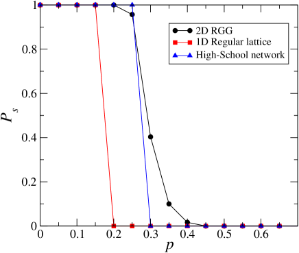
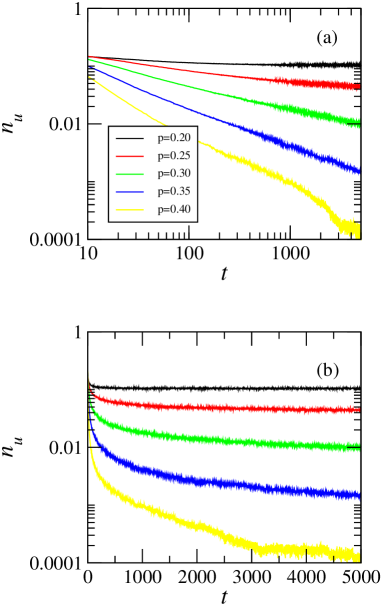
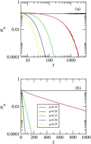
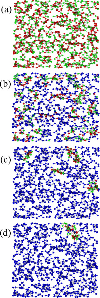
The simulation results (Fig. 10) indicate that the critical point for 2D RGG is significantly higher than that for 1D lattice. For the same choice of $\alpha=1$, the critical point in the case of fully-connected network is $p_{c}\approx 0.27$ (between the values of the 1D and 2D systems). Simulation results plotted in Figs. 11(a) and (b) show that the decay of fraction of unbalanced triangles in the network ($n_{u}$) is governed by the power-law in the case of 2D RGG but it decays exponentially (ignoring the transience) in 1D regular lattice as shown in Figs. 12(a) and (b). In the case of 2D RGG, there are frustrated domains that are long-lived (shown in Fig. 13), whose existence can be causal or symptomatic to the slow convergence. Particular network structure and spatial correlations (among nodes) become significantly important in defining the dynamics of low dimensional systems and a quantitative analysis becomes mathematically challenging.

Figure 11: (Color online) Average fraction of unbalanced triangles in the 2D RGG with $N=1000$, $\langle k\rangle=10$, and $\alpha=1.0$ (a) on a log-log scale and (b) on a semi-log scale. The initial population densities are $x=0.5,y=0.5$.

Figure 12: (Color online) Average fraction of unbalanced triangles in the 1D regular lattice with $N=1000$, $k=10$, and $\alpha=1.0$ (a) on a log-log scale and (b) on a semi-log scale. The initial population densities are $x=0.5,y=0.5$.

Figure 13: (Color online) Time of evolution (single-run) of the system. Green, red, and blue nodes correspond to leftists, rightists, and centrists respectively. The network structure is 2D RGG with $\langle k\rangle=10$, $N=1000$, $\alpha=1.0$, and $p=0.3$. System is initialized with $x=0.5,y=0.5$. (a) $t=0$, (b) $t=10$, (c) $t=100$, and (d) $t=500$, where $t$ is the number of time steps.

IV Summary

In summary, we presented a framework that models social imbalance arising from individual opinions in the simplest manner possible, and observe its counteracting effect on an externally influencing field. We found that there exists a critical value $p_{c}$, above which the only fixed point is the centrist consensus state, and below which a metastable fixed point of the system emerges. We demonstrated how the competition between balance and influence can lead the system to metastability. Using a semi-analytical approach (QS approximation), we estimated the consensus times which show good agreement with simulation results. Additionally, employing simulations, we demonstrated that this critical behavior is also seen in sparse networks.

V Acknowledgements

This work was supported in part by the Army Research Laboratory under Cooperative Agreement Number W911NF-09-2-0053 (the ARL Network Science CTA), by the Office of Naval Research Grant Nos. N00014-09-1-0607 and N00014-15-1-2640, by the Army Research Office grant W911NF-12-1-0546, by the European Commission under the 7th Framework Programme, Grant Agreement Number 316097 [ENGINE], and by the National Science Centre, Poland, the decision no. DEC-2013/09/B/ST6/02317. The views and conclusions contained in this document are those of the authors and should not be interpreted as representing the official policies either expressed or implied of the Army Research Laboratory or the U.S. Government.

Appendix A The $p=0$ case

In this appendix we discuss the $p=0$ case of the model (case with no external influence). When $p=0$, the rate equations for the densities $x$ and $y$ can be written as

$$\frac{dx}{dt} = 3(2\alpha-1)xy(1-x-y)$$

$$\frac{dy}{dt} = 3(2\alpha-1)xy(1-x-y)\;.$$ (14)

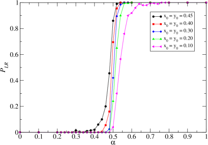
In this case, the entire boundary of the triangular phase space becomes absorbing because structural balance is achieved as soon as either of the $x$, $y$, or $z$ variables becomes zero and from that point the system does not evolve. The type of steady-state (in other other words, which of the three boundaries is hit by the system) of this system depends on the choice of $\alpha$. For $\alpha<\frac{1}{2}$, the system moves towards an all-centrist consensus till it eventually hits either $x=0$ (centrist-leftist coalition) or $y=0$ (centrist-rightist coalition) boundary. However, for $\alpha>\frac{1}{2}$ (in the absence of external field, $p=0$) the system tends to more radical configuration and stops evolving when $x+y=1$ (or reaches the long side of the triangular phase space). After gaining some insight in this case, we performed stochastic simulations. The probability for the system to end up in a polarized state $P_{LR}$ is shown in Fig. 14 (with the complementary probability $P_{CE}=1-P_{LR}$, the system settles in a coalition state).

Figure 14: (Color online) The probability $P_{LR}$ as a function of $\alpha$ for $N=100$ (fully-connected) and different starting points ($p=0$).

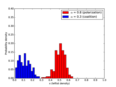
Starting from an equal density initial state ($x_{0}\approx y_{0}\approx z_{0}\approx 0.33$), we also look at the composition of the final state when the system reaches a polarized ($\alpha=0.8$) or a coalition state ($\alpha=0.3$). We only show the distribution of $x$ given that the system reaches a final state on the $y=0$ or $y=1-x$ boundary (Fig. 15). $y$ has the same distribution along $x=0$ and $y=1-x$ boundaries due to symmetry. Starting from an arbitrary state ($x_{0}>0,y_{0}>0,z_{0}>0$), the system never reaches a pure consensus because a structurally balanced configuration is always reached before reaching a pure consensus state and the system freezes in that state. The consensus in this case is observed only if the initial state itself is a consensus state and the system remains in that state.

Figure 15: (Color online) The histogram of leftist density $x$ when the system ends up in a leftist-rightist polarization or centrist-leftist coalition state for $\alpha=0.8$ and $\alpha=0.3$. The network is fully-connected ($N=100$ and $p=0$).

Appendix B Steady-state solution of the rate equations

The rate equations for the leftist and rightist densities under the mean-field assumption are

$$\frac{dx}{dt} = -px+3(2\alpha-1)(1-p)xy(1-x-y)$$

$$\frac{dy}{dt} = -py+3(2\alpha-1)(1-p)xy(1-x-y)\;.$$ (15)

By adding and subtracting the above equations and introducing a new set of variables $u=(x+y)$ and $v=(x-y)$, one can immediately see that

$$\frac{dv}{dt}=-pv\;,$$ (16)

yielding $v\sim\exp(-pt)$, which means that $v\to 0$ exponentially fast. Therefore, we can assume that $x\approx y$ which allows us to analyze the system in terms of single-variable equation for the “slow” mode $u$ (and $x=y=u/2$),

$$\frac{du}{dt}=-pu+6(2\alpha-1)(1-p)\frac{u^{2}(1-u)}{4}\;,$$ (17)

which can be solved for stead-state $\frac{du}{dt}=0$. A trivial solution of this equation is $u=0$, which is the absorbing state ($x=0$, $y=0$). Additional roots are the solutions of the quadratic equation

$$u^{2}-u+\frac{2p}{3(1-p)(2\alpha-1)}=0\;,$$ (18)

and are given by

$$u=\frac{1}{2}\pm\frac{1}{2}\sqrt{1-\frac{8p}{3(1-p)(2\alpha-1)}}\;.$$ (19)

These solutions make sense only when $\alpha>1/2$, otherwise the solution will lie outside the feasible domain [$(x+y)\leq 1$]. For $\alpha>1/2$, we obtain a critical point,

$$p_{c}=\frac{3(2\alpha-1)}{8+3(2\alpha-1)}\;,$$ (20)

such that the roots are real and positive for $p<p_{c}$. Thus, in terms of $x$ and $y$ the two roots (other than the absorbing state) are

$$x=y = \frac{1}{4}+\frac{1}{4}\sqrt{1-\frac{8p}{3(1-p)(2\alpha-1)}}~{}~{}~{}~{}~{}{\rm(metastable)}$$

$$x=y = \frac{1}{4}-\frac{1}{4}\sqrt{1-\frac{8p}{3(1-p)(2\alpha-1)}}~{}~{}~{}~{}~{}{\rm(saddle)}\;.$$ (21)

References

- (1) F. Heider, J. Psychol. 21, 107 (1946).
- (2) S. Wasserman and K. Faust, Social Network Analysis: Methods and Applications (Cambridge University Press, New York, 1994)).
- (3) M. Szell, R. Lambiotte, and S. Thurner, Proc. Natl. Acad. Sci. USA 107, 13636 (2010).
- (4) D. Cartwright and F. Harary, Psychol. Rev. 63, 277 (1956).
- (5) T. Antal, P. L. Krapivsky, and S. Redner, Phys. Rev. E 72, 036121 (2005).
- (6) T. Antal, P. L. Krapivsky, and S. Redner, Physica D: Nonlinear Phenomena 224, 130 (2006).
- (7) S. A. Marvel, S. H. Strogatz, and J. M. Kleinberg, Phys. Rev. Lett. 103, 198701 (2009).
- (8) S. Galam, Physica A 230 (1996).
- (9) G. Vinogradova and S. Galam, Eur. Phys. J. B 87, 266 (2014).
- (10) G. Vinogradova and S. Galam, Journal on Policy and Complex Systems 1, 93 (2014).
- (11) M. Mobilia, J. Stat. Phys. 151, 69 (2013).
- (12) F. Vazquez and S. Redner, J. Phys. A: Mathematical and General 37, 8479 (2004).
- (13) W. Zhang, C. C. Lim, G. Korniss, and B. K. Szymanski, Sci. Rep. 4, 5568 (2014).
- (14) S. A. Marvel, H. Hong, A. Papush, and S. H. Strogatz, Phys. Rev. Lett. 109, 118702 (2012).
- (15) G. Korniss, B. Schmittmann, and R. K. P. Zia, J. Stat. Phys. 86, 721 (1997).
- (16) H. Haken, in Synergetics (Springer Berlin Heidelberg, 2004) pp. 1–387.
- (17) R. Dickman and R. Vidigal, J. Phys. A: Mathematical and General 35, 1147 (2002).
- (18) J. Xie, S. Sreenivasan, G. Korniss, W. Zhang, C. Lim, and B. K. Szymanski, Phys. Rev. E 84, 011130 (2011).
- (19) M. M. de Oliveira and R. Dickman, Physica A: Statistical Mechanics and its Applications 343, 525 (2004).
- (20) J. Xie, J. Emenheiser, M. Kirby, S. Sreenivasan, B.K. Szymanski, and G. Korniss, PLoS One 7(3): e33215 (2012).
- (21) J. Dall and M. Christensen, Phys. Rev. E 66, 016121 (2002).
- (22) P. Singh, S. Sreenivasan, B. K. Szymanski, and G. Korniss, Phys. Rev. E 85, 046104 (2012).
- (23) Add Health was designed by J. Richard Udry, Peter S. Bearman, and Kathleen Mullan Harris, and funded by a grant P01-HD31921 from the National Institute of Child Health and Human Development, with cooperative funding from 17 other agencies. For data files contact Add Health, Carolina Population Center, 123 W. Franklin Street, Chapel Hill, NC 27516-2524, addhealth@unc.edu, http://www.cpc.unc.edu/projects/addhealth/ (Accessed March 22, 2016).