Bound-constrained polynomial optimization using only elementary calculations

Etienne de Klerk and Jean B. Lasserre and Monique Laurent and Zhao Sun Tilburg University and Delft University of Technology; PO Box 90153, 5000 LE Tilburg, The Netherlands. E.deKlerk@uvt.nl LAAS-CNRS and Institute of Mathematics, University of Toulouse, LAAS, 7 avenue du Colonel Roche, 31077 Toulouse CΓ©dex 4, France, Tel: +33561336415 lasserre@laas.fr Centrum Wiskunde & Informatica (CWI), Amsterdam and Tilburg University; CWI, Postbus 94079, 1090 GB Amsterdam, The Netherlands. M.Laurent@cwi.nl Γ‰cole Polytechnique de MontrΓ©al; Canada Excellence Research Chair in Data Science for Real-Time Decision-Making, C.P. 6079, Succ. Centre-ville, Montr al, H3C 3A7, Canada. Zhao.Sun@polymtl.ca
Abstract.

We provide a monotone non-increasing sequence of upper bounds $f^{H}_{k}$ ($k\geq 1$) converging to the global minimum of a polynomial $f$ on simple sets like the unit hypercube in $\mathbb{R}^{n}$. The novelty with respect to the converging sequence of upper bounds in [J.B. Lasserre, A new look at nonnegativity on closed sets and polynomial optimization, SIAM J. Optim. 21, pp. 864–885, 2010] is that only elementary computations are required. For optimization over the hypercube $[0,1]^{n}$, we show that the new bounds $f^{H}_{k}$ have a rate of convergence in $O(1/\sqrt{k})$. Moreover we show a stronger convergence rate in $O(1/k)$ for quadratic polynomials and more generally for polynomials having a rational minimizer in the hypercube. In comparison, evaluation of all rational grid points with denominator $k$ produces bounds with a rate of convergence in $O(1/k^{2})$, but at the cost of $O(k^{n})$ function evaluations, while the new bound $f^{H}_{k}$ needs only $O(n^{k})$ elementary calculations.

Key words and phrases:
Polynomial optimization and bound-constrained optimization and Lasserre hierarchy
2000 Mathematics Subject Classification:
90C22 and 90C26 and 90C30

1. Introduction

Consider the problem of computing the global minimum

(1.1) $$f_{\min,{\mathcal{K}}}\>=\,\min\,\{f(\mathbf{x}):\>\mathbf{x}\in{\mathcal{K}}\,\},$$

of a polynomial $f$ on a compact set ${\mathcal{K}}\subset\mathbb{R}^{n}$. (We will mainly deal with the case where ${\mathcal{K}}$ is a basic semi-algebraic set.)

A fruitful perspective, introduced by Lasserre [16], is to reformulate problem (1.1) as

$$f_{\min,{\mathcal{K}}}=\inf_{\mathbf{\mu}}\int_{{\mathcal{K}}}fd\mathbf{\mu},$$

where the infimum is taken over all probability measures $\mu$ with support in ${\mathcal{K}}$. Using this reformulation one may obtain a sequence of lower bounds on $f_{\min,{\mathcal{K}}}$ that converges to $f_{\min,{\mathcal{K}}}$, by introducing tractable convex relaxations of the set of probability measures with support in ${\mathcal{K}}$ (if ${\mathcal{K}}$ is semi-algebraic). For more details on this approach the interested reader is referred to Lasserre [15, 16, 18], and [20, 17] for a comparison between linear programming (LP) and semidefinite programming (SDP) relaxations.

As an alternative, one may obtain a sequence of upper bounds by optimizing over specific classes of probability distributions. In particular, Lasserre [19] defined the sequence (also called hierarchy) of upper bounds

(1.2) fks​o​s:=minΟƒβˆˆΞ£k​[𝐱]⁑{βˆ«π’¦f​(𝐱)​σ​(𝐱)​𝑑𝐱:βˆ«π’¦Οƒβ€‹(𝐱)​𝑑𝐱=1},(k=1,2,…),assignsuperscriptsubscriptπ‘“π‘˜π‘ π‘œπ‘ subscript𝜎subscriptΞ£π‘˜delimited-[]𝐱:subscriptπ’¦π‘“π±πœŽπ±differential-d𝐱subscriptπ’¦πœŽπ±differential-d𝐱1π‘˜12…f_{k}^{sos}:=\min_{\sigma\in\Sigma_{k}[\mathbf{x}]}\left\{\int_{{\mathcal{K}}}f(\mathbf{x})\sigma(\mathbf{x})d\mathbf{x}\;:\;\int_{{\mathcal{K}}}\sigma(\mathbf{x})d\mathbf{x}=1\right\},\quad(k=1,2,\ldots),

where $\Sigma_{k}[\mathbf{x}]$ denotes the cone of sums of squares (SOS) of polynomials of degree at most $2k$. Thus the optimization is restricted to probability distributions where the probability density function is an SOS polynomial of degree at most $2k$. Lasserre [19] showed that fks​o​sβ†’fmin,𝒦→superscriptsubscriptπ‘“π‘˜π‘ π‘œπ‘ subscript𝑓𝒦f_{k}^{sos}\rightarrow f_{\min,{\mathcal{K}}} as $k\rightarrow\infty$ (see Theorem 2.1 below for a precise statement). In principle this approach works for any compact set ${\mathcal{K}}$ and any polynomial but for practical implementation it requires knowledge of moments of the measure $\sigma(\mathbf{x})d\mathbf{x}$. So in practice the approach is limited to simple sets ${\mathcal{K}}$ like the Euclidean ball, the hypersphere, the simplex, the hypercube and/or their image by a linear transformation.

In fact computing such upper bounds reduces to computing the smallest generalized eigenvalue associated with two real symmetric matrices whose size increases in the hierarchy. For more details the interested reader is referred to Lasserre [19]. In a recent paper, De Klerk et al. [6] have provided the first convergence analysis for this hierarchy and shown a bound fks​o​sβˆ’fmin,𝒦=O​(1/k)superscriptsubscriptπ‘“π‘˜π‘ π‘œπ‘ subscript𝑓𝒦𝑂1π‘˜f_{k}^{sos}-f_{\min,{\mathcal{K}}}=O(1/\sqrt{k}) on the rate of convergence. In a related analysis of convergence Romero and Velasco [23] provide a bound on the rate at which one may approximate from outside the cone of nonnegative homogeneous polynomials (of fixed degree) by the hierarchy of spectrahedra defined in [19].

It should be emphasized that it is a difficult challenge in optimization to obtain a sequence of upper bounds converging to the global minimum and having a known estimate on the rate of convergence. So even if the convergence to the global minimum of the hierarchy of upper bounds obtained in [19] is rather slow, and even though it applies to the restricted context of β€œsimple sets”, to the best of our knowledge it provides one of the first results of this kind. A notable earlier result was obtained for polynomial optimization over the simplex, where it has been shown that brute force grid search leads to a polynomial time approximation scheme for minimizing polynomials of fixed degree [1, 4]. When minimizing over the set of grid points in the standard simplex with given denominator $k$, the rate of convergence is in $O(1/k)$ [1, 4] and, for quadratic polynomials (and for general polynomials having a rational minimizer), in $O(1/k^{2})$ [5]. Grid search over the hypercube was also shown to have a rate of convergence in $O(1/k)$ [3] and, as we will indicate in this paper, a stronger rate of convergence in $O(1/k^{2})$ can be shown. Note however that computing the best grid point in the hypercube $[0,1]^{n}$ with denominator $k$ requires $O(k^{n})$ computations, thus exponential in the dimension.

Contribution

As our main contribution we provide a monotone non-increasing converging sequence $(f^{H}_{k})_{k\in\mathbb{N}}$, of upper bounds $f^{H}_{k}\geq f_{\min,{\mathcal{K}}}$ such that $f^{H}_{k}\to f_{\min,{\mathcal{K}}}$ as $k\to\infty$. The parameters $f^{H}_{k}$ can be effectively computed when the set ${\mathcal{K}}\subseteq[0,1]^{n}$ is a β€œsimple set” like, for example, a Euclidean ball, sphere, simplex, hypercube, or any linear transformation of them.

This β€œhierarchy” of upper bounds is inspired from the one defined by Lasserre in [19], but with the novelty that:

Computing the upper bounds $(f^{H}_{k})$ does not require solving an SDP or computing the smallest generalized eigenvalue of some pair of matrices (as is the case in [19]). It only requires elementary calculations (but possibly many of them for good quality bounds).

Indeed, computing the upper bound $f^{H}_{k}$ only requires finding the minimum in a list of $O(n^{k})$ scalars $(\gamma_{(\eta,\beta)})$, formed from the moments $\boldsymbol{\gamma}$ of the Lebesgue measure on the set ${\mathcal{K}}\subseteq[0,1]^{n}$ and from the coefficients $(f_{\alpha})$ of the polynomial $f$ to minimize. Namely:

(1.3) $$f^{H}_{k}\,:=\,\displaystyle\min_{(\eta,\beta)\in\mathbb{N}^{2n}_{k}}\>\sum_{\alpha\in\mathbb{N}^{n}}f_{\alpha}\,\frac{\gamma_{(\eta+\alpha,\beta)}}{\gamma_{(\eta,\beta)}},$$

where $\mathbb{N}$ denotes the nonnegative integers, $f(\mathbf{x})=\sum_{\alpha\in\mathbb{N}^{n}}f_{\alpha}\,\mathbf{x}^{\alpha}$, $\mathbb{N}^{2n}_{k}=\{(\eta,\beta)\in\mathbb{N}^{2n}:|\eta+\beta|=k\}$, and the scalars

$$\gamma_{(\eta,\beta)}\,:=\,\int_{\mathcal{K}}x_{1}^{\eta_{1}}\cdots x_{n}^{\eta_{n}}(1-x_{1})^{\beta_{1}}\cdots(1-x_{n})^{\beta_{n}}\,d\mathbf{x},\quad(\eta,\beta)\in\mathbb{N}^{2n},$$

are available in closed-form. (Our informal notion of β€œsimple set” therefore means that the moments $\gamma_{(\eta,\beta)}$ are known a priori.)

The upper bound (1.3) has also a simple interpretation as it reads:

(1.4) $$f^{H}_{k}=\,\displaystyle\min_{(\eta,\beta)\in\mathbb{N}^{2n}_{k}}\>\frac{\displaystyle\int_{\mathcal{K}}f(\mathbf{x})\,\mathbf{x}^{\eta}(\mathbf{1}-\mathbf{x})^{\beta}\,d\mathbf{x}}{\displaystyle\int_{\mathcal{K}}\mathbf{x}^{\eta}(\mathbf{1}-\mathbf{x})^{\beta}\,d\mathbf{x}}\,=\,\displaystyle\min_{\mu}\,\left\{\displaystyle\,\int_{\mathcal{K}}f\,d\mu:\>\mu\in M({\mathcal{K}})_{k}\,\right\},$$

where $M({\mathcal{K}})_{k}$ is the set of probability measures on ${\mathcal{K}}$, absolutely continuous with respect to the Lebesgue measure on ${\mathcal{K}}$, and whose density is a monomial $\mathbf{x}^{\eta}(\mathbf{1}-\mathbf{x})^{\beta}$ with $(\eta,\beta)\in\mathbb{N}^{2n}_{k}$. (Such measures are in fact products of (univariate) beta distributions, see Section 4.1.) This also proves that at any point $\mathbf{a}\in[0,1]^{n}$ one may approximate the Dirac measure $\delta_{\mathbf{a}}$ with measures of the form $d\mu=\mathbf{x}^{\eta}(\mathbf{1}-\mathbf{x})^{\beta}\,d\mathbf{x}$ (normalized to make then probability measures).

For the case of the hypercube ${\mathcal{K}}=[0,1]^{n}$, we analyze the rate of convergence of the bounds $f^{H}_{k}$ and show a rate of convergence in $O(1/\sqrt{k})$ for general polynomials, and in $O(1/k)$ for quadratic polynomials (and general polynomials having a rational minimizer). As a second minor contribution, we revisit grid search over the rational points with given denominator $k$ in the hypercube and observe that its convergence rate is in $O(1/k^{2})$ (which follows as an easy application of Taylor’s theorem). However as observed earlier the computation of the best grid point with denominator $k$ requires $O(k^{n})$ function evaluations while the computation of the parameter $f^{H}_{k}$ requires only $O(n^{k})$ elementary calculations.

Organization of the paper.

We start with some basic facts about the bounds $f^{H}_{k}$ in Section 2 and in Section 3 we show their convergence to the minimum of $f$ over the set ${\mathcal{K}}$ (see Theorem 3.1).

In Section 4, for the case of the hypercube ${\mathcal{K}}=[0,1]^{n}$, we analyze the quality of the bounds $f^{H}_{k}$. We show a convergence rate in $O(1/\sqrt{k})$ for the range $f^{H}_{k}-f_{\min,{\mathcal{K}}}$ and a stronger convergence rate in $O(1/k)$ when the polynomial $f$ admits a rational minimizer in $[0,1]^{n}$ (see Theorem 4.9). This stronger convergence rate applies in particular to quadratic polynomials (since they have a rational minimizer) and Example 4.10 shows that this bound is tight. When no rational minimizer exists the weaker rate follows using Diophantine approximations. So again the main message of this paper is that one may obtain non-trivial upper bounds with error guarantees (and converging to the global minimum) via elementary calculations and without invoking a sophisticated algorithm.

In Section 5 we revisit the simple technique which consists of evaluating the polynomial $f$ at all rational points in $[0,1]^{n}$ with given denominator $k$. By a simple application of Taylor’s theorem we can show a convergence rate in $O(1/k^{2})$. However, in terms of computational complexity, the parameters $f^{H}_{k}$ are easier to compute. Indeed, for fixed $k$, computing $f^{H}_{k}$ requires $O(n^{k})$ computations (similar to function evaluations), while computing the minimum of $f$ over all grid points with given denominator $k$ requires an exponential number $k^{n}$ of function evaluations.

In Section 6 we present some additional (simple) techniques to provide a feasible point $\hat{\mathbf{x}}\in{\mathcal{K}}$ with value $f(\hat{\mathbf{x}})\leq f^{H}_{k}$, once the upper bound $f^{H}_{k}$ has been computed, hence also with an error bound guarantee in the case of the box ${\mathcal{K}}=[0,1]^{n}$. This includes, in the case when $f$ is convex, getting a feasible point using Jensen inequality (Section 6.1) and, in the general case, taking the mode $\hat{\mathbf{x}}$ of the optimal density function (i.e., its global maximizer) (see Section 6.2).

In Section 7, we present some numerical experiments, carried out on several test functions on the box $[0,1]^{n}$. In particular, we compare the values of the new bound $f^{H}_{k}$ with the bound fk/2s​o​ssubscriptsuperscriptπ‘“π‘ π‘œπ‘ π‘˜2f^{sos}_{k/2} (whose definition uses a sum of squares density), and we apply the proposed techniques to find a feasible point in the box. As expected the sos based bound is tighter in most cases but the bound $f^{H}_{k}$ can be computed for much larger values of $k$. Moreover, the feasible points $\hat{\mathbf{x}}$ returned by the proposed mode heuristic are often of very good quality for sufficiently large $k$. Finally, in Section 8 we conclude with some remarks on variants of the bound $f^{H}_{k}$ that may offer better results in practice.

2. Notation, definitions and preliminary results

Throughout we let $\mathbb{R}[\mathbf{x}]$ denote the ring of polynomials in the variables $\mathbf{x}=(x_{1},\ldots,x_{n})$, $\mathbb{R}[\mathbf{x}]_{d}$ is the subspace of polynomials of degree at most $d$, and $\Sigma[\mathbf{x}]_{d}\subset\mathbb{R}[\mathbf{x}]_{2d}$ is its subset of sums of squares (SOS) of degree at most $2d$.

We use the convention that $\mathbb{N}$ denotes the set of nonnegative integers, and set $\mathbb{N}^{n}_{d}:=\{\alpha\in\mathbb{N}^{n}:\sum_{i=1}^{n}\alpha_{i}\,(=:|\alpha|)=d\}$, and similarly $\mathbb{N}^{n}_{\leq d}:=\{\alpha\in\mathbb{N}^{n}:\sum_{i=1}^{n}\alpha_{i}\,\leq d\}$. The notation $\mathbf{x}^{\alpha}$ stands for the monomial $x_{1}^{\alpha_{1}}\cdots x_{n}^{\alpha_{n}}$, while $(\mathbf{1}-\mathbf{x})^{\alpha}$ stands for $(1-x_{1})^{\alpha_{1}}\cdots(1-x_{n})^{\alpha_{n}}$, $\alpha\in\mathbb{N}^{n}$. We will also denote $[n]=\{1,2,\ldots,n\}$ and let $\mathbf{1}$ denote the all-ones vector (of suitable size).

One may write every polynomial $f\in\mathbb{R}[\mathbf{x}]_{d}$ in the monomial basis

$$\mathbf{x}\mapsto f(\mathbf{x})\,=\,\sum_{\alpha\in\mathbb{N}^{n}_{\leq d}}f_{\alpha}\,\mathbf{x}^{\alpha},$$

with vector of (finitely many) coefficients $(f_{\alpha})$.

2.1. The bounds fks​o​ssubscriptsuperscriptπ‘“π‘ π‘œπ‘ π‘˜f^{sos}_{k} and $f^{H}_{k}$

In [19], Lasserre introduced the parameters fks​o​ssubscriptsuperscriptπ‘“π‘ π‘œπ‘ π‘˜f^{sos}_{k} as upper bounds for the minimum $f_{\min,{\mathcal{K}}}$ of $f$ over ${\mathcal{K}}$ and he proved the following result.

Theorem 2.1 (Lasserre [19]).

Let ${\mathcal{K}}\subseteq\mathbb{R}^{n}$ be compact, let $f_{\min,{\mathcal{K}}}$ be as in (1.1), and let

(2.1) fks​o​s:=infΟƒ{βˆ«π’¦f​(𝐱)​σ​(𝐱)​𝑑𝐱:βˆ«π’¦Οƒβ€‹(𝐱)​𝑑𝐱=1,ΟƒβˆˆΞ£β€‹[𝐱]k},kβˆˆβ„•.formulae-sequenceassignsubscriptsuperscriptπ‘“π‘ π‘œπ‘ π‘˜subscriptinfimum𝜎conditional-setsubscriptπ’¦π‘“π±πœŽπ±differential-d𝐱formulae-sequencesubscriptπ’¦πœŽπ±differential-d𝐱1𝜎Σsubscriptdelimited-[]π±π‘˜π‘˜β„•f^{sos}_{k}\,:=\,\inf_{\sigma}\,\left\{\displaystyle\int_{\mathcal{K}}f(\mathbf{x})\,\sigma(\mathbf{x})\,d\mathbf{x}:\>\displaystyle\int_{\mathcal{K}}\sigma(\mathbf{x})\,d\mathbf{x}=1,\sigma\in\Sigma[\mathbf{x}]_{k}\,\right\},\quad k\in\mathbb{N}.

Then fmin,𝒦≀fk+1s​o​s≀fks​o​ssubscript𝑓𝒦subscriptsuperscriptπ‘“π‘ π‘œπ‘ π‘˜1subscriptsuperscriptπ‘“π‘ π‘œπ‘ π‘˜f_{\min,{\mathcal{K}}}\,\leq\,f^{sos}_{k+1}\,\leq\,f^{sos}_{k} for all $k$ and

(2.2) fmin,𝒦=limkβ†’βˆžfks​o​s.subscript𝑓𝒦subscriptβ†’π‘˜subscriptsuperscriptπ‘“π‘ π‘œπ‘ π‘˜f_{\min,{\mathcal{K}}}\,=\,\displaystyle\lim_{k\to\infty}\>f^{sos}_{k}.

We will also use the following important result due to Krivine [13, 14] and Handelman [10].

Theorem 2.2.

Let ${\mathcal{K}}=\{\mathbf{x}:g_{j}(\mathbf{x})\geq 0,\>j=1,\dots,m\}\subset\mathbb{R}^{n}$ be a polytope with a nonempty interior and where each $g_{j}$ is an affine polynomial, $j=1,\ldots,m$. If $f\in\mathbb{R}[\mathbf{x}]$ is strictly positive on ${\mathcal{K}}$ then

(2.3) $$f(\mathbf{x})\,=\,\sum_{\alpha\in\mathbb{N}^{m}}\lambda_{\alpha}\,g_{1}(\mathbf{x})^{\alpha_{1}}\cdots g_{m}(\mathbf{x})^{\alpha_{m}},\qquad\forall\mathbf{x}\in\mathbb{R}^{n},$$

for finitely many positive scalars $\lambda_{\alpha}$.

We will call the expression in (2.3) the Handelman representation of $f$, and call any $f$ that allows a Handelman representation to be of the Handelman type. Throughout we consider the following set of polynomials:

(2.4) $${\mathcal{H}}_{k}:=\left\{p\in\mathbb{R}[\mathbf{x}]:p(\mathbf{x})=\sum_{(\eta,\beta)\in\mathbb{N}^{2n}_{k}}\lambda_{\eta,\beta}\mathbf{x}^{\eta}(\mathbf{1}-\mathbf{x})^{\beta}\ \ \text{ where }\lambda_{\eta\beta}\geq 0\right\},$$

i.e., all polynomials that admit a Handelman representation of degree at most $k$ in terms of the polynomials $x_{i},1-x_{i}$ defining the hypercube $[0,1]^{n}$.

Observe that any term $\mathbf{x}^{\eta}(\mathbf{1}-\mathbf{x})^{\beta}$ with degree $|\eta+\beta|<k$ also belongs to the set ${\mathcal{H}}_{k}$. This follows by iteratively applying the identity: $1=x_{i}+(1-x_{i})$, which permits to rewrite $\mathbf{x}^{\eta}(\mathbf{1}-\mathbf{x})^{\beta}$ as a conic combination of terms $\mathbf{x}^{\eta^{\prime}}(\mathbf{1}-\mathbf{x})^{\beta^{\prime}}$ with degree $|\eta^{\prime}+\beta^{\prime}|=k$. The next claim follows then as a direct application.

Lemma 2.3.

We have the inclusion: ${\mathcal{H}}_{k}\subseteq{\mathcal{H}}_{k+1}$ for all $k$.

We may now interpret the new upper bounds $f^{H}_{k}$ from (1.3) in an analogous way as the bounds fks​o​ssubscriptsuperscriptπ‘“π‘ π‘œπ‘ π‘˜f^{sos}_{k} from (2.1), but where the SOS density function $\sigma\in\Sigma_{k}[\mathbf{x}]$ is now replaced by a density $\sigma\in{\mathcal{H}}_{k}$.

For clarity we first repeat the definition (1.3) of the parameters $f^{H}_{k}$ below:

$$f^{H}_{k}\,:=\,\displaystyle\min_{(\eta,\beta)\in\mathbb{N}^{2n}_{k}}\>\sum_{\alpha\in\mathbb{N}^{n}}f_{\alpha}\,\frac{\gamma_{(\eta+\alpha,\beta)}}{\gamma_{(\eta,\beta)}},$$

where the scalars

$$\gamma_{(\eta,\beta)}\,=\,\int_{\mathcal{K}}\mathbf{x}^{\eta}(\mathbf{1}-\mathbf{x})^{\beta}d\mathbf{x}=\,\int_{\mathcal{K}}x_{1}^{\eta_{1}}\cdots x_{n}^{\eta_{n}}(1-x_{1})^{\beta_{1}}\cdots(1-x_{n})^{\beta_{n}}\,dx_{1}\cdots dx_{n},\quad(\eta,\beta)\in\mathbb{N}^{2n},$$

denote the moments of the Lebesgue measure on the set $\mathcal{K}$. Using the fact that

$$\sum_{\alpha\in\mathbb{N}^{n}}f_{\alpha}\gamma_{(\eta+\alpha,\beta)}=\sum_{\alpha\in\mathbb{N}^{n}}f_{\alpha}\int_{\mathcal{K}}\mathbf{x}^{\eta+\alpha}(\mathbf{1}-\mathbf{x})^{\beta}d\mathbf{x}=\int_{\mathcal{K}}f(\mathbf{x})\mathbf{x}^{\eta}(\mathbf{1}-\mathbf{x})^{\beta}d\mathbf{x},$$

we can rewrite the parameter $f^{H}_{k}$ as in (1.4):

$$f^{H}_{k}=\,\displaystyle\min_{(\eta,\beta)\in\mathbb{N}^{2n}_{k}}\>\frac{\displaystyle\int_{\mathcal{K}}f(\mathbf{x})\,\mathbf{x}^{\eta}(\mathbf{1}-\mathbf{x})^{\beta}\,d\mathbf{x}}{\displaystyle\int_{\mathcal{K}}\mathbf{x}^{\eta}(\mathbf{1}-\mathbf{x})^{\beta}\,d\mathbf{x}}.$$

We now give yet another reformulation for the parameter $f^{H}_{k}$, where we optimize over density functions in the set $\mathcal{H}_{k}$, which turn out to be convex combinations of density functions of the form $\mathbf{x}^{\eta}(\mathbf{1}-\mathbf{x})^{\beta}$ (after suitable scaling).

Lemma 2.4.

Let ${\mathcal{K}}\subseteq[0,1]^{n}$, let $f$ be a polynomial, and consider the parameters $f^{H}_{k}$, $k\in\mathbb{N}$, from (1.3). Then one has:

$$f^{H}_{k}=\,\inf_{\sigma\in{\mathcal{H}}_{k}\,}\,\left\{\displaystyle\int_{\mathcal{K}}f(\mathbf{x})\,\sigma(\mathbf{x})\,d\mathbf{x}:\>\displaystyle\int_{\mathcal{K}}\sigma(\mathbf{x})\,d\mathbf{x}=1\right\}\quad\text{ for all }k\in\mathbb{N},$$

and the sequence $(f^{H}_{k})_{k}$ is monotonically non-increasing: $f^{H}_{k+1}\leq f^{H}_{k}$.

Proof.

Note that, for given $k\in\mathbb{N}$,

$\displaystyle\inf_{\sigma}\,\left\{\displaystyle\int_{\mathcal{K}}f(\mathbf{x})\,\sigma(\mathbf{x})\,d\mathbf{x}:\>\displaystyle\int_{\mathcal{K}}\sigma(\mathbf{x})\,d\mathbf{x}=1,\;\sigma\in{\mathcal{H}}_{k}\,\right\}$
$\displaystyle=$ $\displaystyle\inf_{\lambda\geq 0}\left\{\sum_{\alpha\in\mathbb{N}^{n}_{d}}f_{\alpha}\left(\sum_{(\eta,\beta)\in\mathbb{N}^{2n}_{k}}\lambda_{\eta\beta}\,\underbrace{\int_{\mathcal{K}}\mathbf{x}^{\eta+\alpha}(\mathbf{1}-\mathbf{x})^{\beta}\,d\mathbf{x}}_{\gamma_{(\eta+\alpha,\beta)}}\right):\sum_{(\eta,\beta)\in\mathbb{N}^{2n}_{k}}\lambda_{\eta\beta}\underbrace{\int_{\mathcal{K}}\mathbf{x}^{\eta}(\mathbf{1}-\mathbf{x})^{\beta}\,d\mathbf{x}}_{\gamma_{(\eta,\beta)}}=1\right\}$
$\displaystyle=$ $\displaystyle\displaystyle\inf_{\lambda\geq 0}\left\{\displaystyle\sum_{(\eta,\beta)\in\mathbb{N}^{2n}_{k}}\lambda_{\eta\beta}\,\left(\displaystyle\sum_{\alpha\in\mathbb{N}^{n}_{d}}f_{\alpha}\,\gamma_{(\eta+\alpha,\beta)}\right):\quad\displaystyle\sum_{(\eta,\beta)\in\mathbb{N}^{2n}_{k}}\lambda_{\eta\beta}\,\gamma_{(\eta,\beta)}=1\right\}$
$\displaystyle=$ $\displaystyle\displaystyle\min_{(\eta,\beta)\in\mathbb{N}^{2n}_{k}}\>\sum_{\alpha\in\mathbb{N}^{n}_{d}}f_{\alpha}\,\frac{\gamma_{(\eta+\alpha,\beta)}}{\gamma_{(\eta,\beta)}}=f^{H}_{k},$

where we have used the fact that the penultimate optimization problem is an LP over a simplex that attains its infimum at one of the vertices. The monotonicity of the sequence $(f^{H}_{k})_{k\in\mathbb{N}}$ now follows from Lemma 2.3. ∎

2.2. Calculating moments on ${\mathcal{K}}$

For ${\mathcal{K}}\subseteq[0,1]^{n}$ a compact set and for every $(\eta,\beta)\in\mathbb{N}^{2n}$, we need to calculate the parameters

(2.5) $$\gamma_{(\eta,\beta)}\,:=\,\int_{\mathcal{K}}\mathbf{x}^{\eta}(\mathbf{1}-\mathbf{x})^{\beta}\,d\mathbf{x},$$

in order to compute $f^{H}_{k}$. When ${\mathcal{K}}$ is arbitrary one does not know how to compute such generalized moments. But if ${\mathcal{K}}$ is the unit hypercube $[0,1]^{n}$, the simplex $\Delta:=\{\mathbf{x}:\mathbf{x}\geq 0;\,\sum_{i=1}^{n}x_{i}\leq 1\}$, a Euclidean ball (or sphere), and/or their image by a linear mapping, then such moments are available in closed-form; see e.g.Β [19]. We give the moments for the hypercube ${\mathcal{K}}=[0,1]^{n}$, which we will treat in detail in this paper. Namely,

$$\int_{[0,1]^{n}}\mathbf{x}^{\eta}\,(\mathbf{1}-\mathbf{x})^{\beta}\,d\mathbf{x}\,=\,\prod_{i=1}^{n}\displaystyle\left(\displaystyle{\int_{0}^{1}x_{i}^{\eta_{i}}(1-x_{i})^{\beta_{i}}\,dx_{i}}\right),\quad\text{ for any }(\eta,\beta)\in\mathbb{N}^{2n},$$

and the univariate integrals may be calculated from

(2.6) $$\int_{0}^{1}t^{i}(1-t)^{j}\,dt={i!j!\over(i+j+1)!},\quad\quad\text{ for any }i,j\in\mathbb{N}.$$

2.3. The complexity of computing $f_{k}^{H}$ and fks​o​ssuperscriptsubscriptπ‘“π‘˜π‘ π‘œπ‘ f_{k}^{sos}

We let $N_{f}$ denote the set of indices $\alpha\in\mathbb{N}^{n}$ for which fΞ±β‰ 0subscript𝑓𝛼0f_{\alpha}\neq 0; note that $|N_{f}|\leq{n+d\choose d}$ if $d$ is the total degree of $f$. The computation of $f_{k}^{H}$ is done by computing the summations:

$$\sum_{\alpha\in N_{f}}f_{\alpha}\,\frac{\gamma_{(\eta+\alpha,\beta)}}{\gamma_{(\eta,\beta)}}$$

for all $(\eta,\beta)\in\mathbb{N}^{2n}_{k}$, and taking the minimum one. (We assume that the values $\gamma_{(\eta,\beta)}$ are pre-computed for all $(\eta,\beta)\in\mathbb{N}^{2n}_{k+d}$.)

Thus, for fixed $(\eta,\beta)\in\mathbb{N}^{2n}_{k}$, one may first compute the inner product of the vectors with components $f_{\alpha}$ and $\gamma_{(\eta+\alpha,\beta)}$ (indexed by $\alpha$). Note that these vectors are of size $|N_{f}|$. Since there are ${2n+k-1\choose k}$ pairs $(\eta,\beta)\in\mathbb{N}^{2n}_{k}$, the entire computation requires $(2|N_{f}|+1){2n+k-1\choose k}$ flops111We define floating point operations (flops) as in [9, p. 18]; in particular, by this definition the inner product of two $n$-vectors requires $2n$ flops..

As explained in [19], the computation of the upper bounds fks​o​ssuperscriptsubscriptπ‘“π‘˜π‘ π‘œπ‘ f_{k}^{sos} may be done by finding the smallest generalized eigenvalue $\lambda$ of the system:

A​x=λ​B​x(xβ‰ 0),𝐴π‘₯πœ†π΅π‘₯π‘₯0Ax=\lambda Bx\quad\quad\quad(x\neq 0),

for suitable symmetric matrices $A$ and $B$ of order ${n+k\choose k}$. In particular, the rows and columns of the two matrices are indexed by $\mathbb{N}^{n}_{\leq k}$, and

$$A_{\alpha,\beta}=\sum_{\delta\in N_{f}}f_{\delta}\int_{{\mathcal{K}}}\mathbf{x}^{\alpha+\beta+\delta}d\mathbf{x},\quad B_{\alpha,\beta}=\int_{{\mathcal{K}}}\mathbf{x}^{\alpha+\beta}d\mathbf{x}\quad\alpha,\beta\in\mathbb{N}^{n}_{\leq k}.$$

Note that the matrices $A$ and $B$ depend on the moments of the Lebesgue measure on ${\mathcal{K}}$, and that these moments may be computed beforehand, by assumption. One may compute $A_{\alpha,\beta}$ by taking the inner product of $(f_{\delta})_{\delta\in N_{f}}$ with the vector of moments $\left(\int_{{\mathcal{K}}}\mathbf{x}^{\alpha+\beta+\delta}d\mathbf{x}\right)_{\delta\in N_{f}}$. Thus computation of the elements of $A$ require a total of $|N_{f}|\left({n+k\choose k}+1\right)^{2}$ flops.

Also note that the matrix $B$ is a positive definite (Gram) matrix. Thus one has to solve a so-called symmetric-definite generalized eigenvalue problem, and this may be done in $14{n+k\choose k}^{3}$ flops; see e.g.Β [9, Section 8.7.2]. Thus one may compute fks​o​ssuperscriptsubscriptπ‘“π‘˜π‘ π‘œπ‘ f_{k}^{sos} in at most $14{n+k\choose k}^{3}+|N_{f}|\left({n+k\choose k}+1\right)^{2}$ flops.

2.4. An illustrating example

We give an example to illustrate the behaviour of the bounds fks​o​ssubscriptsuperscriptπ‘“π‘ π‘œπ‘ π‘˜f^{sos}_{k} and $f^{H}_{k}$. More examples will be given in Section 7.

Example 2.5.

As an example we consider the bivariate Styblinski-Tang function

$$f(x_{1},x_{2})=\sum_{i=1}^{2}{1\over 2}(10x_{i}-5)^{4}-8(10x_{i}-5)^{2}+{5\over 2}(10x_{i}-5)$$

over the square ${\mathcal{K}}=[0,1]^{2}$, with minimum $f_{\min,{\mathcal{K}}}\approx-78.33198$ and minimizer

$$\mathbf{x}^{*}\approx(0.20906466,0.20906466).$$

Using a SOS density function, the upper bound of degree 2 is f1s​o​s=βˆ’12.9249superscriptsubscript𝑓1π‘ π‘œπ‘ 12.9249f_{1}^{sos}=-12.9249, and the corresponding optimal SOS density of degree $2$ is (roughly)

$$\sigma(x_{1},x_{2})=(1.9169-1.005x_{1}-1.005x_{2})^{2}.$$

Using a Handelman-type density function, the upper bound of degree $2$ is $f^{H}_{2}=-17.3810$, with corresponding optimal density

$\displaystyle\sigma(x_{1},x_{2})=6x_{2}(1-x_{2}).$

On the other hand, if we consider densities of degree $6$ then we get f3s​o​s=βˆ’34.403superscriptsubscript𝑓3π‘ π‘œπ‘ 34.403f_{3}^{sos}=-34.403 and $f^{H}_{6}=-31.429$.

Thus there is no general ordering between the bounds fks​o​ssuperscriptsubscriptπ‘“π‘˜π‘ π‘œπ‘ f_{k}^{sos} and $f_{2k}^{H}$. Having said that, we will show in Section 7 that, for most of the examples we have considered, one has fks​o​s≀f2​kHsuperscriptsubscriptπ‘“π‘˜π‘ π‘œπ‘ superscriptsubscript𝑓2π‘˜π»f_{k}^{sos}\leq f_{2k}^{H} for all $k$, as one may expect from the relative computational efforts.

Refer to caption
Refer to caption
Figure 1. Optimal Handelman-type density $\sigma$ of degree $50$ on $[0,1]^{2}$ for the bivariate Styblinski-Tang function.

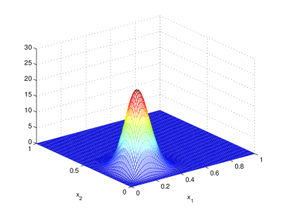
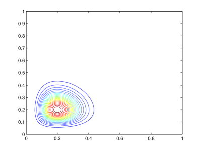
As a final illustration, Figure 1 shows the plot and contour plot of the Handelman-type density corresponding to the bound $f_{50}^{H}=-60.536$ (i.e.Β degree $50$).

The figure illustrates the earlier assertion that the optimal density approximates the Dirac delta measure at the minimizer $\mathbf{x}^{*}\approx(0.20906466,0.20906466)$. Indeed, it is clear from the contour plot that the mode of the optimal density is close to $\mathbf{x}^{*}$.

3. Convergence proof for the bounds $f^{H}_{k}$ on ${\mathcal{K}}\subseteq[0,1]^{n}$

In this section we prove the convergence of the sequence $({f^{H}_{k}})_{k\in\mathbb{N}}$ to the minimum of $f$ over any compact set ${\mathcal{K}}\subseteq[0,1]^{n}$.

Theorem 3.1.

Let ${\mathcal{K}}\subseteq[0,1]^{n}$, let $f\in\mathbb{R}[\mathbf{x}]_{d}$ and let $\gamma_{(\eta,\beta)}$ be as in (2.5). Define as in (1.3) the parameters

(3.1) $$f^{H}_{k}\,=\,\displaystyle\min_{(\eta,\beta)\in\mathbb{N}^{2n}_{k}}\>\sum_{\alpha\in\mathbb{N}^{n}_{\leq d}}f_{\alpha}\,\frac{\gamma_{(\eta+\alpha,\beta)}}{\gamma_{(\eta,\beta)}},\qquad\forall\,k\in\mathbb{N}.$$

Then, $f_{\min,{\mathcal{K}}}=\displaystyle\lim_{k\to\infty}f^{H}_{k}$.

Proof.

As in (1.2), let fks​o​ssuperscriptsubscriptπ‘“π‘˜π‘ π‘œπ‘ f_{k}^{sos} denote the bound obtained by searching over an SOS density $\sigma$ of degree at most $2k$:

fks​o​s=minβ€‹βˆ«π’¦f​(𝐱)​σ​(𝐱)​𝑑𝐱​ such thatΒ β€‹βˆ«π’¦Οƒβ€‹(𝐱)​𝑑𝐱=1,ΟƒβˆˆΞ£β€‹[𝐱]k.formulae-sequencesuperscriptsubscriptπ‘“π‘˜π‘ π‘œπ‘ subscriptπ’¦π‘“π±πœŽπ±differential-d𝐱 such thatΒ subscriptπ’¦πœŽπ±differential-d𝐱1𝜎Σsubscriptdelimited-[]π±π‘˜f_{k}^{sos}=\min\int_{{\mathcal{K}}}f(\mathbf{x})\sigma(\mathbf{x})d\mathbf{x}\ \text{ such that }\int_{{\mathcal{K}}}\sigma(\mathbf{x})d\mathbf{x}=1,\ \sigma\in\Sigma[\mathbf{x}]_{k}.

Also recall from Lemma 2.4 that

$$f^{H}_{k}=\min\int_{{\mathcal{K}}}f(\mathbf{x})\sigma(\mathbf{x})d\mathbf{x}\ \ \text{such that }\int_{{\mathcal{K}}}\sigma(\mathbf{x})d\mathbf{x}=1,\ \sigma\in{\mathcal{H}}_{k}.$$

By Lemma 2.4, the sequence $(f^{H}_{k})$ is monotone non-increasing, with $f_{\min,{\mathcal{K}}}\leq f^{H}_{k}$ for all $k$. Hence it has a limit which is at least $f_{\min,{\mathcal{K}}}$, we now show that the limit is equal to $f_{\min,{\mathcal{K}}}$.

To this end, let $\epsilon>0$. As the sequence (fks​o​s)subscriptsuperscriptπ‘“π‘ π‘œπ‘ π‘˜(f^{sos}_{k}) converges to $f_{\min,{\mathcal{K}}}$ (Theorem 2.1), there exists an integer $k$ such that

fmin,𝒦≀fks​o​s≀fmin,𝒦+Ο΅.subscript𝑓𝒦subscriptsuperscriptπ‘“π‘ π‘œπ‘ π‘˜subscript𝑓𝒦italic-Ο΅f_{\min,{\mathcal{K}}}\leq f^{sos}_{k}\leq f_{\min,{\mathcal{K}}}+\epsilon.

Next, there exists a polynomial $\sigma\in\Sigma_{k}$ such that $\int_{{\mathcal{K}}}\sigma(\mathbf{x})d\mathbf{x}=1$ and

fks​o​sβ‰€βˆ«π’¦f​(𝐱)​σ​(𝐱)​𝑑𝐱≀fks​o​s+Ο΅.subscriptsuperscriptπ‘“π‘ π‘œπ‘ π‘˜subscriptπ’¦π‘“π±πœŽπ±differential-d𝐱subscriptsuperscriptπ‘“π‘ π‘œπ‘ π‘˜italic-Ο΅f^{sos}_{k}\leq\int_{{\mathcal{K}}}f(\mathbf{x})\sigma(\mathbf{x})d\mathbf{x}\leq f^{sos}_{k}+\epsilon.

Define now the polynomial $\hat{\sigma}(\mathbf{x})=\sigma(\mathbf{x})+\epsilon$. Then $\hat{\sigma}$ is strictly positive on $[0,1]^{n}$ and thus, by Theorem 2.2 applied to the hypercube $[0,1]^{n}$, $\hat{\sigma}\in{\mathcal{H}}_{j_{k}}$ for some integer $j_{k}$. Observe that

$$\int_{{\mathcal{K}}}\hat{\sigma}(\mathbf{x})d\mathbf{x}=\int_{{\mathcal{K}}}(\sigma(\mathbf{x})+\epsilon)d\mathbf{x}\geq\int_{{\mathcal{K}}}\sigma(\mathbf{x})d\mathbf{x}=1.$$

Hence we obtain:

$$f^{H}_{j_{k}}-f_{\min,{\mathcal{K}}}\leq{\int_{{\mathcal{K}}}f(\mathbf{x})\hat{\sigma}(\mathbf{x})d\mathbf{x}\over\int_{{\mathcal{K}}}\hat{\sigma}(\mathbf{x})d\mathbf{x}}-f_{\min,{\mathcal{K}}}={\int_{{\mathcal{K}}}(f(\mathbf{x})-f_{\min,{\mathcal{K}}})\hat{\sigma}(\mathbf{x})d\mathbf{x}\over\int_{{\mathcal{K}}}\hat{\sigma}(\mathbf{x})d\mathbf{x}}\leq\int_{{\mathcal{K}}}(f(\mathbf{x})-f_{\min,{\mathcal{K}}})\hat{\sigma}(\mathbf{x})d\mathbf{x}.$$

The right most term is equal to

$$\int_{{\mathcal{K}}}(f(\mathbf{x})-f_{\min,{\mathcal{K}}})\sigma(\mathbf{x})d\mathbf{x}+\epsilon\int_{{\mathcal{K}}}(f(\mathbf{x})-f_{\min,{\mathcal{K}}})d\mathbf{x}=\int_{{\mathcal{K}}}f(\mathbf{x})\sigma(\mathbf{x})d\mathbf{x}-f_{\min,{\mathcal{K}}}+\epsilon\int_{{\mathcal{K}}}(f(\mathbf{x})-f_{\min,{\mathcal{K}}})d\mathbf{x},$$

where we used the fact that $\int_{{\mathcal{K}}}\sigma(\mathbf{x})d\mathbf{x}=1$. Finally, combining with the fact that βˆ«π’¦f​(𝐱)​σ​(𝐱)​𝑑𝐱≀fks​o​s+ϡ≀fmin,𝒦+2​ϡsubscriptπ’¦π‘“π±πœŽπ±differential-d𝐱superscriptsubscriptπ‘“π‘˜π‘ π‘œπ‘ italic-Ο΅subscript𝑓𝒦2italic-Ο΅\int_{{\mathcal{K}}}f(\mathbf{x})\sigma(\mathbf{x})d\mathbf{x}\leq f_{k}^{sos}+\epsilon\leq f_{\min,{\mathcal{K}}}+2\epsilon, we can derive that

$$f^{H}_{j_{k}}-f_{\min,{\mathcal{K}}}\leq\epsilon\left(2+\int_{{\mathcal{K}}}(f(\mathbf{x})-f_{\min,{\mathcal{K}}})d\mathbf{x}\right)=\epsilon C,$$

where $C:=2+\int_{{\mathcal{K}}}(f(\mathbf{x})-f_{\min,{\mathcal{K}}})d\mathbf{x}$ is a constant. This concludes the proof. ∎

Note that, in the proof, it was essential to have $\hat{\sigma}$ strictly positive on all of $[0,1]^{n}$, for the application of Handelman’s theorem. The fact that $\hat{\sigma}(\mathbf{x})=\sigma(\mathbf{x})+\epsilon$ with $\sigma$ SOS and $\epsilon>0$ guaranteed this strict positivity.

4. Bounding the rate of convergence for the parameters $f^{H}_{k}$ on ${\mathcal{K}}=[0,1]^{n}$

In this section we analyze the rate of convergence of the bounds $f^{H}_{k}$ for the hypercube ${\mathcal{K}}=[0,1]^{n}$. We prove a convergence rate in $O(1/\sqrt{k})$ for the range $f^{H}_{k}-f_{\min,{\mathcal{K}}}$ in general, and a stronger convergence rate in $O(1/k)$ when $f$ has a rational global minimizer in $[0,1]^{n}$, which is the case, for instance, when $f$ is quadratic.

Our main tool will be exploiting some properties of the moments $\gamma_{(\eta,\beta)}$ which, as we recall below, arise from the moments of the beta distribution.

4.1. Properties of the beta distribution

By definition, a random variable $X\in[0,1]$ has the beta distribution with shape parameters $a>0$ and $b>0$, which is denoted by $X\sim beta(a,b)$, if its probability density function is given by

$$y\mapsto\frac{y^{a-1}(1-y)^{b-1}}{\int_{0}^{1}t^{a-1}(1-t)^{b-1}dt}.$$

If $a>1$ and $b>1$, then the (unique) mode of the distribution (i.e.,Β the maximizer of the density function) is

(4.1) $$y=(a-1)/(a+b-2).$$

Moreover, the $k$-th moment of $X$ is given by

(4.2) $$\mathbb{E}(X^{k})={a(a+1)\cdots(a+k-1)\over(a+b)(a+b+1)\cdots(a+b+k-1)},\quad(k=1,2,3,\ldots)$$

(see, e.g, [12, Chapter 24]; this also follows using (2.6)).

In what follows we will consider families of random random variables with the beta distribution of the form $X\sim beta(ar,br)$, where $a$ and $b$ are positive real numbers and $r\geq 1$ is an integer. By (4.2), any such random variable has mean

$$\mathbb{E}(X)=\frac{ar}{ar+br}=\frac{a}{a+b}.$$

In Lemma 4.2 below we show how the moments of such random variables relate to powers of the mean. The proof relies on the following technical lemma.

Lemma 4.1.

Let $k$ be a positive integer. There exists a constant $C_{k}>0$ (depending only on $k$) for which the following relation holds:

(4.3) $${rp(rp+1)\cdots(rp+k-1)\over rq(rq+1)\cdots(rq+k-1)}-{p^{k}\over q^{k}}\leq{C_{k}\over r}$$

for all integers $r\geq 1$, and real numbers $0<p<q$.

Proof.

Consider the univariate polynomial $\phi(t)=(t+1)\cdots(t+k-1)=\sum_{i=0}^{k-1}a_{i}t^{i}$, where the scalars $a_{i}>0$ depend only on $k$ and $a_{k-1}=1$. Denote by $\Delta$ the left hand side in (4.3), which can be written as $\Delta=N/D$, where we set

$$N:=rpq^{k}\phi(rp)-rqp^{k}\phi(rq),\ \ \ D:=rq^{k+1}\phi(rq).$$

We first work out the term $N$:

$$N=rpq\left(\sum_{i=0}^{k-2}a_{i}r^{i}p^{i}q^{k-1}-\sum_{i=0}^{k-2}a_{i}r^{i}q^{i}p^{k-1}\right)=rpq\sum_{i=0}^{k-2}a_{i}r^{i}p^{i}q^{i}(q^{k-1-i}-p^{k-1-i}).$$

Write: $q^{k-1-i}-p^{k-1-i}=(q-p)\sum_{j=0}^{k-2-i}q^{j}p^{k-2-i-j}\leq(q-p)q^{k-2-i}(k-1-i)$, where we use the fact that $p<q$. This implies:

$$N\leq rpq(q-p)\sum_{i=0}^{k-2}a_{i}r^{i}p^{i}q^{k-2}(k-1-i)=rpq^{k-1}(q-p)\sum_{i=0}^{k-2}a_{i}(k-1-i)r^{i}p^{i}=:N^{\prime}.$$

Thus we get:

$$\Delta\leq{N^{\prime}\over D}={p(q-p)\over q^{2}}\cdot{\sum_{i=0}^{k-2}a_{i}(k-1-i)r^{i}p^{i}\over\phi(rq)}.$$

The first factor is at most 1, since one has: $p(q-p)\leq q^{2}$, as $q^{2}-p(q-p)=(q-p)^{2}+pq$. Second, we bound the sum $\sum_{i=0}^{k-2}a_{i}(k-1-i)r^{i}p^{i}$ in terms of $\phi(rq)=\sum_{j=0}^{k-1}a_{j}r^{j}q^{j}.$ Namely, define the constant

$$C_{k}:=\max_{0\leq i\leq k-2}{a_{i}(k-1-i)\over a_{i+1}},$$

which depends only on $k$. We show that

$$a_{i}(k-1-i)r^{i}p^{i}\leq{C_{k}\over r}.$$

Indeed, for each $0\leq i\leq k-2$, using $p^{i}\leq q^{i+1}$ and the definition of $C_{k}$, we get:

$$r\cdot a_{i}(k-1-i)r^{i}p^{i}\leq a_{i}(k-1-i)r^{i+1}q^{i+1}\leq C_{k}a_{i+1}r^{i+1}q^{i+1}.$$

Summing over $i=0,1,\ldots,k-2$ gives:

$$r\sum_{i=0}^{k-2}a_{i}(k-1-i)r^{i}p^{i}\leq C_{k}\sum_{i=0}^{k-2}a_{i+1}r^{i+1}q^{i+1}\leq C_{k}\phi(rq),$$

and thus

$$\Delta\leq{N^{\prime}\over D}\leq{C_{k}\over r}$$

as desired. ∎

Lemma 4.2.

For any integer $k\geq 1$, there exists a constant $C^{\prime}_{k}>0$ (depending only on $k$) for which the following holds:

$$\left|\mathbb{E}(X^{k})-(\mathbb{E}(X))^{k}\right|\leq{C^{\prime}_{k}\over r},$$

for all integers $r\geq 1$, real numbers $a,b>0$, and where $X\sim beta(ar,br)$.

Proof.

Directly using (4.2), $\mathbb{E}(X)={a\over a+b}$, and Lemma 4.1 applied to $p=a$ and $q=a+b$. ∎

Now we consider i.i.d.Β random variables $X_{1},\ldots,X_{n}$ such that

(4.4) $$X_{i}\sim beta(a_{i}r,b_{i}r)\quad a_{i},b_{i}>0\;(i\in[n]),\;r\geq 1,r\in\mathbb{N},$$

and denote $X=(X_{1},\ldots,X_{n})$. For given $\alpha\in\mathbb{N}^{n}$, we denote $X^{\alpha}=\prod_{i=1}^{n}X_{i}^{\alpha_{i}}$. Since the random variables $X_{i}$ are independent we have $\mathbb{E}(X^{\alpha})=\prod_{i=1}^{n}\mathbb{E}(X_{i}^{\alpha_{i}})$ and, for a polynomial $f=\sum f_{\alpha}\mathbf{x}^{\alpha}$, the expected value of $f(X)=\sum_{\alpha\in{\mathbb{N}}^{n}}f_{\alpha}X^{\alpha}$ is given by

(4.5) $$\mathbb{E}(f(X))=\sum_{\alpha\in{\mathbb{N}}^{n}}f_{\alpha}\mathbb{E}(X^{\alpha})=\sum_{\alpha\in{\mathbb{N}}^{n}}f_{\alpha}\prod_{i=1}^{n}\mathbb{E}(X_{i}^{\alpha_{i}}).$$

Recall that the explicit value of $\mathbb{E}(X_{i}^{\alpha_{i}})$ is given by (4.2). The next result relates $\mathbb{E}(f(X))$ (the expected value of $f(X)$) and $f(\mathbb{E}(X))$ (the value of $f$ evaluated at the mean of $X$).

Lemma 4.3.

Let $f(\mathbf{x})=\sum_{\alpha\in{\mathbb{N}}^{n}}f_{\alpha}\mathbf{x}^{\alpha}$ and $X=(X_{1},\ldots,X_{n})$, where the i.i.d.Β random variables $X_{i}$ $(i\in[n])$ are as in (4.4). Then there is a constant $\hat{C}_{f}>0$ (depending on $f$ only) such that

$$|\mathbb{E}(f(X))-f\left(\mathbb{E}(X)\right)|\leq\frac{\hat{C}_{f}}{r}.$$
Proof.

We have

$\displaystyle\mathbb{E}(f(X))-f(\mathbb{E}(X))=\sum_{\alpha\in{\mathbb{N}}^{n}}f_{\alpha}{\left(\prod_{i=1}^{n}\mathbb{E}(X_{i}^{\alpha_{i}})-\prod_{i=1}^{n}(\mathbb{E}(X_{i}))^{\alpha_{i}}\right)}.$

By the identity:

(4.6) $$\prod_{i=1}^{n}x_{i}-\prod_{i=1}^{n}y_{i}=\sum_{i=1}^{n}\left[(x_{i}-y_{i})\prod_{j=1}^{i-1}y_{j}\prod_{j=i+1}^{n}x_{j}\right]\quad\quad(\mathbf{x},\mathbf{y}\in\mathbb{R}^{n}),$$

one has

$\displaystyle\prod_{i=1}^{n}\mathbb{E}(X_{i}^{\alpha_{i}})-\prod_{i=1}^{n}(\mathbb{E}(X_{i}))^{\alpha_{i}}=\sum_{i=1}^{n}\left(\left(\mathbb{E}(X_{i}^{\alpha_{i}})-(\mathbb{E}(X_{i}))^{\alpha_{i}}\right){\prod_{j=1}^{i-1}(\mathbb{E}(X_{j}))^{\alpha_{j}}}{\prod_{j=i+1}^{n}\mathbb{E}(X_{j}^{\alpha_{j}})}\right).$

Since $\mathbb{E}(X_{i})\in[0,1]$ and $\mathbb{E}(X_{i}^{\alpha_{i}})\in[0,1]$ for any $i\in[n]$, it follows that

$\displaystyle|\mathbb{E}(f(X))-f(\mathbb{E}(X))|$ $\displaystyle\leq$ $\displaystyle\sum_{\alpha\in{\mathbb{N}}^{n}}\left|f_{\alpha}\right|\sum_{i=1}^{n}\left|\mathbb{E}(X_{i}^{\alpha_{i}})-(\mathbb{E}(X_{i}))^{\alpha_{i}}\right|$
$\displaystyle\leq$ $\displaystyle\sum_{\alpha\in{\mathbb{N}}^{n}}\left|f_{\alpha}\right|\sum_{i=1}^{n}{C^{\prime}_{\alpha_{i}}\over r},$

where the second inequality is from Lemma 4.2, and the constant $C^{\prime}_{\alpha_{i}}>0$ only depends on $\alpha_{i}$. Setting $\hat{C}_{f}:=\sum_{\alpha\in\mathbb{N}^{n}}|f_{\alpha}|\sum_{i=1}^{n}C^{\prime}_{\alpha_{i}}$ concludes the proof. ∎

4.2. Proof of the convergence rate

Let $\mathbf{x}^{*}$ be a global minimizer of $f$ in $[0,1]^{n}$. Our objective is to analyze the rate of convergence of the sequence $(f^{H}_{k}-f(\mathbf{x}^{*}))_{k}$. Our strategy is to define suitable shape parameters $\eta^{*}_{i},\beta^{*}_{i}$ from the components $x^{*}_{i}$ of the global minimizer $\mathbf{x}^{*}$ so that, if we choose a vector $X=(X_{1},\ldots,X_{n})$ of i.i.d. random variables with $X_{i}\sim beta(\eta^{*}_{i},\beta^{*}_{i})$, then (roughly) $\mathbb{E}(X)\approx\mathbf{x}^{*}$ and $\mathbb{E}(f(X))\approx f^{H}_{k}$ (so that we can use the result of Lemma 4.3 to estimate $f^{H}_{k}-f(\mathbf{x}^{*})$.

In a first step we indicate how to define the shape parameters $\eta^{*}_{i},\beta^{*}_{i}$. For any given integer $r\geq 1$ we will select them of the form $\eta^{*}_{i}=ra_{i}$, $\beta^{*}_{i}=rb_{i}$, where $a_{i},b_{i}$ are constructed from the coordinates of $\mathbf{x}^{*}$. As we want $\eta^{*}_{i},\beta^{*}_{i}$ to be integer valued we need to discuss whether a coordinate $x_{i}$ is rational or not, and to deal with irrational coordinates we will use the following result about Diophantine approximations.

Theorem 4.4 (Dirichlet’s theorem).

(See e.g. [24, Chapter 6.1]) Consider a real number $x\in\mathbb{R}$ and $0<\epsilon\leq 1$. Then there exist integers $p$ and $q$ satisfying

|xβˆ’pq|<Ο΅q​ and ​ 1≀q≀1Ο΅.π‘₯π‘π‘žitalic-Ο΅π‘žΒ andΒ 1π‘ž1italic-Ο΅\left|x-{p\over q}\right|<{\epsilon\over q}\ \text{ and }\ 1\leq q\leq{1\over\epsilon}.

If $x\in(0,1)$, then one may moreover assume $0\leq p\leq q$.

Definition 4.5 (Shape parameters for rational components).

Fix an integer $r\geq 1$. For rational coordinates $x^{*}_{i}\in\mathbb{Q}$ define $\eta_{i}^{*}$, $\beta^{*}_{i}$ as follows:

  • (i)

    If $x^{*}_{i}=0$ then set $\eta^{*}_{i}=1$ and $\beta^{*}_{i}=r$.

  • (ii)

    If $x_{i}^{*}=1$ then set $\eta^{*}_{i}=r$ and $\beta^{*}_{i}=1$.

  • (iii)

    If $x^{*}_{i}\in\mathbb{Q}\setminus\{0,1\}$ then write $x^{*}_{i}=p_{i}/q_{i}$ where $1\leq p_{i}<q_{i}$ are integers, and set $\eta^{*}_{i}=rp_{i}$ and $\beta^{*}_{i}=r(q_{i}-p_{i})$.

Definition 4.6 (Shape parameters for irrational components).

Fix an integer $r\geq 1$. For each irrational coordinate $x^{*}_{i}\in\mathbb{R}\setminus\mathbb{Q}$, apply Theorem 4.4 with $\epsilon=1/r$ to obtain integers $p_{i},q_{i}$ satisfying

$$\left|x_{i}^{*}-{p_{i}\over q_{i}}\right|<{1\over rq_{i}},\ 0\leq p_{i}\leq q_{i}\leq r,\ \text{and}\ 1\leq q_{i}.$$

Define the sets $I_{0}=\{i\in[n]:x_{i}^{*}\in\mathbb{R}\setminus\mathbb{Q},\ p_{i}=0\},\ I_{1}=\{i\in[n]:x_{i}^{*}\in\mathbb{R}\setminus\mathbb{Q},\ p_{i}=q_{i}\},$ and $I=\{i\in[n]:x_{i}^{*}\in\mathbb{R}\setminus\mathbb{Q},\ 1\leq p_{i}<q_{i}\}$, and define $\eta^{*}_{i}$, $\beta^{*}_{i}$ as follows:

  • (iv)

    If $i\in I_{0}$ then set $\eta^{*}_{i}=1$ and $\beta^{*}_{i}=r$.

  • (v)

    If $i\in I_{1}$ then set $\eta^{*}_{i}=r$ and $\beta^{*}_{i}=1$.

  • (vi)

    If $i\in I$ then set $\eta^{*}_{i}=rp_{i}$ and $\beta^{*}_{i}=r(q_{i}-p_{i})$.

As above consider i.i.d. $X=(X_{1},\ldots,X_{n})$, where $X_{i}\sim beta(\eta^{*}_{i},\beta^{*}_{i})$. Then, by construction, for all $i\in[n]$, one has

$$\mathbb{E}(X_{i})=\frac{\eta_{i}^{*}}{\eta_{i}^{*}+\beta_{i}^{*}}=\left\{\begin{array}[]{ll}\frac{1}{r+1}&\mbox{in cases (i), (iv),}\\ \frac{r}{r+1}&\mbox{in cases (ii), (v),}\\ \frac{p_{i}}{q_{i}}&\mbox{in cases (iii), (vi).}\\ \end{array}\right.$$

One can verify that in all cases one has

(4.7) $$|\mathbb{E}(X_{i})-x_{i}^{*}|\leq 1/r\ \text{ for all }i\in[n].$$

Observe morever that, again by construction,

(4.8) $$\mathbb{E}(f(X))={\int_{[0,1]^{n}}f(\mathbf{x})\mathbf{x}^{\eta^{*}-\mathbf{1}}(\mathbf{1}-\mathbf{x})^{\beta^{*}-\mathbf{1}}d\mathbf{x}\over\int_{[0,1]^{n}}\mathbf{x}^{\eta^{*}-\mathbf{1}}(\mathbf{1}-\mathbf{x})^{\beta^{*}-\mathbf{1}}d\mathbf{x}}\geq f^{H}_{k_{r}}\geq f(\mathbf{x}^{*})\ ,$$

where we let $\mathbf{1}$ denote the all-ones vector and we define the parameter

(4.9) $$k_{r}:=\sum_{i=1}^{n}(\eta_{i}^{*}-1+\beta_{i}^{*}-1).$$

We will use the following estimate on the parameter $k_{r}$.

Lemma 4.7.

Consider the parameter $k_{r}=\sum_{i=1}^{n}(\eta_{i}^{*}-1+\beta_{i}^{*}-1)$ and $J=\{i\in[n]:x^{*}_{i}\in\mathbb{Q}\setminus\{0,1\}\}$. Then the following holds:

  • (a)

    If $\mathbf{x}^{*}\in\mathbb{Q}^{n}$ then $k_{r}\leq ar$ for all $r\geq 1$, where $a>0$ is a constant (not depending on $r$).

  • (b)

    If $\mathbf{x}^{*}\not\in\mathbb{Q}^{n}$ then $k_{r}\leq a^{\prime}r^{2}$ for all $r\geq 1$, where $a^{\prime}>0$ is a constant (not depending on $r$).

  • (c)

    For $r=1$, we have that $k_{1}=\sum_{i\in J}q_{i}-2|J|$.

Proof.

By construction, $\eta_{i}^{*}+\beta_{i}^{*}-2=rq_{i}-2$ for each $i\in I\cup J$, and $\eta_{i}^{*}+\beta_{i}^{*}-2=r-1$ otherwise. From this one gets $k_{r}=r(\sum_{i\in I\cup J}q_{i}+n-|I\cup J|)-n-|I\cup J|=:ar-b$, after setting $b:=n+|I\cup J|$ and $a:=\sum_{i\in I\cup J}q_{i}+n-|I\cup J|$, so that $a,b\geq 0$. Thus, $k_{r}\leq ar$ holds.

Next, note that $q_{i}\leq r$ for each $i\in I$, while $q_{i}$ does not depend on $r$ for $i\in J$ (since then $x_{i}^{*}=p_{i}/q_{i}$). Hence, in case (a), $I=\emptyset$ and the constant $a$ does not depend on $r$. In case (b), we obtain: $a\leq r|I|+\sum_{i\in J}q_{i}+n-|I\cup J|\leq a^{\prime}r$, after setting $a^{\prime}:=|I|+\sum_{i\in J}q_{i}+n-|I\cup J|$, which is thus a constant not depending on $r$. Then, $k_{r}\leq ar\leq a^{\prime}r^{2}$.

In the case $r=1$, the set $I$ is empty and thus $k_{1}=\sum_{i\in J}q_{i}-2|J|$, showing (c). ∎

We can now prove the following upper bound for the range $\mathbb{E}(f(X))-f(\mathbf{x}^{*})$ (thus also for the range $f^{H}_{k_{r}}-f(\mathbf{x}^{*})$) which will be crucial for establishing the rate of convergence of the parameters $f^{H}_{k}$.

Theorem 4.8.

Given a polynomial $f$ of total degree $d$, consider a global minimizer $\mathbf{x}^{*}$ of $f$ in $[0,1]^{n}$. Let $r$ be a positive integer. For any $x_{i}^{*}\in[0,1]$ ($i\in[n]$), consider the parameters $\eta_{i}^{*},\beta_{i}^{*}$ as in Definitions 4.5 and 4.6, and i.i.d. random variables $X_{i}\sim beta(\eta^{*}_{i},\beta^{*}_{i})$. Then there exists a constant $C_{f}>0$ (depending only on $f$) such that

$\displaystyle f^{H}_{k_{r}}-f(\mathbf{x}^{*})\leq\mathbb{E}(f(X))-f(\mathbf{x}^{*})\leq{C_{f}\over r},$

where $k_{r}$ is as in (4.9).

Proof.

The leftmost inequality follows using (4.8), we show the rightmost one. By Lemma 4.3 one has:

$\displaystyle\mathbb{E}(f(X))-f(\mathbf{x}^{*})$ $\displaystyle=$ $\displaystyle\mathbb{E}(f(X))-f(\mathbb{E}(X))+f(\mathbb{E}(X))-f(\mathbf{x}^{*})$
$\displaystyle\leq$ $\displaystyle\hat{C}_{f}/r+f(\mathbb{E}(X))-f(\mathbf{x}^{*}),$

where $\hat{C}_{f}>0$ is a constant that depends on $f$ only. Thus we need only bound $f(\mathbb{E}(X))-f(\mathbf{x}^{*})$. To this end, note that

$\displaystyle f(\mathbb{E}(X))-f(\mathbf{x}^{*})$ $\displaystyle=$ $\displaystyle\sum_{\alpha\in{\mathbb{N}}^{n}}f_{\alpha}{\left(\prod_{i=1}^{n}\mathbb{E}(X_{i})^{\alpha_{i}}-\prod_{i=1}^{n}(x^{*}_{i})^{\alpha_{i}}\right)}.$

Using again the identity (4.6) one has

$$\left|\left(\prod_{i=1}^{n}\mathbb{E}(X_{i})^{\alpha_{i}}-\prod_{i=1}^{n}(x^{*}_{i})^{\alpha_{i}}\right)\right|\leq\sum_{i:\alpha_{i}>0}|\mathbb{E}(X_{i})-x_{i}^{*}|\leq\frac{d}{r},$$

where $d$ is the degree of $f$, and we have used $|\mathbb{E}(X_{i})-x_{i}^{*}|\leq 1/r$, $x_{i}^{*}\in[0,1]$ and $\mathbb{E}(X_{i})\in[0,1]$ for all $i\in[n]$. Setting

$$C_{f}=\hat{C}_{f}+{d\sum_{\alpha\in{\mathbb{N}}^{n}}|f_{\alpha}|}$$

completes the proof. ∎

Finally we can now show the following for the rate of convergence of the sequence $f^{H}_{k}$, which is our main result.

Theorem 4.9.

Let $f$ be a polynomial, let $\mathbf{x}^{*}$ be a global minimizer of $f$ in $[0,1]^{n}$, and consider as before the parameters

$$f^{H}_{k}=\,\min_{(\eta,\beta)\in\mathbb{N}_{k}^{2n}}\>\frac{\int_{[0,1]^{n}}f(\mathbf{x})\,\mathbf{x}^{\eta}(\mathbf{1}-\mathbf{x})^{\beta}\,d\mathbf{x}}{\int_{[0,1]^{n}}\mathbf{x}^{\eta}(\mathbf{1}-\mathbf{x})^{\beta}\,d\mathbf{x}}\quad(k=1,2,\ldots).$$

There exists a constant $M_{f}$ (depending only on $f$) such that

(4.10) $$f^{H}_{k}-f(\mathbf{x}^{*})\leq{M_{f}\over\sqrt{k}}\ \ \text{ for all }k\geq k_{1},$$

where $k_{1}=\sum_{i\in J}q_{i}-2|J|$, with $J=\{i\in[n]:x^{*}_{i}\in\mathbb{Q}\setminus\{0,1\}\}$ and $x_{i}^{*}=p_{i}/q_{i}$ for integers $1\leq p_{i}<q_{i}$ if $i\in J$. Moreover, if $f$ has at least one rational global minimizer $\mathbf{x}^{*}$, then there exists a constant $M^{\prime}_{f}$ (depending only on $f$) such that

(4.11) $$f^{H}_{k}-f(\mathbf{x}^{*})\leq{M^{\prime}_{f}\over k}\ \ \text{ for all }k\geq k_{1}.$$

In particular, the convergence rate is in $O(1/k)$ when $f$ is a quadratic polynomial.

Proof.

Consider an arbitrary integer $k\geq k_{1}$. Let $r\geq 1$ be the largest integer for which $k\geq k_{r}$. Then we have $k_{r}\leq k<k_{r+1}$. As $k_{r}\leq k$, we have the inequality $f^{H}_{k}\leq f^{H}_{k_{r}}$ and thus, by TheoremΒ 4.8, we obtain

$$f^{H}_{k}-f(\mathbf{x}^{*})\leq f^{H}_{k_{r}}-f(\mathbf{x}^{*})\leq{C_{f}\over r},$$

where the constant $C_{f}$ depends only on $f$.

If $\mathbf{x}^{*}\in\mathbb{Q}^{n}$ then, by Lemma 4.7 (a), $k_{r+1}\leq a(r+1)\leq 2ar$. This implies $k\leq k_{r+1}\leq 2ar$, where the constant $a$ does not depend on $r$. Thus,

fkHβˆ’f​(π±βˆ—)≀Cfr≀2​a​Cfk=Mfk,subscriptsuperscriptπ‘“π»π‘˜π‘“superscript𝐱subscriptπΆπ‘“π‘Ÿ2π‘ŽsubscriptπΆπ‘“π‘˜subscriptπ‘€π‘“π‘˜f^{H}_{k}-f(\mathbf{x}^{*})\leq{C_{f}\over r}\leq{2aC_{f}\over k}{\color[rgb]{0,0,0}\definecolor[named]{pgfstrokecolor}{rgb}{0,0,0}\pgfsys@color@gray@stroke{0}\pgfsys@color@gray@fill{0}={M_{f}\over k}},

where the constant $M_{f}={2aC_{f}}$ depends only on $f$. This shows (4.11).

If $\mathbf{x}^{*}\not\in\mathbb{Q}^{n}$ then, by Lemma 4.7 (b), $k_{r+1}\leq a^{\prime}(r+1)^{2}\leq 4a^{\prime}r^{2}$. This implies $k\leq k_{r+1}\leq 4a^{\prime}r^{2}$ and thus ${1\over r}\leq{2\sqrt{a^{\prime}}\over\sqrt{k}}$, where the constant $a^{\prime}$ does not depend on $r$. Therefore,

$$f^{H}_{k}-f(\mathbf{x}^{*})\leq{C_{f}\over r}\leq{2\sqrt{a^{\prime}}C_{f}\over\sqrt{k}}={M^{\prime}_{f}\over\sqrt{k}},$$

where the constant $M^{\prime}_{f}=2\sqrt{a^{\prime}}C_{f}$ depends only on $f$. This shows (4.10).

Finally, if $f$ is quadratic then, by a result of Vavasis [25], $f$ has a rational minimizer over the hypercube and thus the rate of convergence is $O(1/k)$. ∎

Note that the inequalities (4.10) and (4.11) hold for all $k\geq k_{1}$, where $k_{1}$ depends only on the rational components in $(0,1)$ of the minimizer $\mathbf{x}^{*}$. The constant $k_{1}$ can be in $O(1)$, e.g., when all but $O(1)$ of these rational components have a small denominator (say, equal to $2$). Thus we can, for some problem classes, get a bound with an error estimate in polynomial time.

Example 4.10.

Consider the polynomial $f=\sum_{i=1}^{n}x_{i}$ and the set ${\mathcal{K}}=[0,1]^{n}$. Then $f_{min,{\mathcal{K}}}=0$ is attained at $\mathbf{x}^{*}=0$. Using the relations (2.5), (2.6) and (3.1), it follows that

$$f_{k}^{H}=\min_{(\eta,\beta)\in\mathbb{N}^{2n}_{k}}\sum_{i=1}^{n}{\eta_{i}+1\over\eta_{i}+\beta_{i}+2}.$$

Since $\eta_{i}+\beta_{i}\leq k$ and $\eta_{i}\geq 0$ (for any $i\in[n]$), we have $f_{k}^{H}\geq{n\over k+2}$.

By this example, there does not exist any $\delta>0$ such that, for any $f$, $f_{k}^{H}-f_{\min,{\mathcal{K}}}=O(1/k^{1+\delta}).$ Therefore, when a rational minimizer exists, the convergence rate from Theorem 4.9 in $O(1/k)$ for $f_{k}^{H}$ is tight.

5. Bounding the rate of convergence for grid search over ${\mathcal{K}}=[0,1]^{n}$

As an alternative to computing $f^{H}_{k}$ on ${\mathcal{K}}=Q:=[0,1]^{n}$, one may minimize $f$ over the regular grid:

$$Q(k):=\{\mathbf{x}\in Q=[0,1]^{n}\mid k\mathbf{x}\in\mathbb{N}^{n}\},$$

i.e.,Β the set of rational points in $[0,1]^{n}$ with denominator $k$. Thus we get the upper bound

$$f_{\min,Q(k)}:=\min_{\mathbf{x}\in Q(k)}f(x)\geq f_{\min,Q}\quad k=1,2,\ldots$$

De Klerk and Laurent [3] showed a rate of convergence in $O(1/k)$ for this sequence of upper bounds:

(5.1) $$f_{\min,Q(k)}-f_{\min,Q}\leq{L(f)\over k}{d+1\choose 3}n^{d}\ \text{ for any }k\geq d,$$

where $d$ is the degree of $f$ and $L(f)$ is the constant

$$L(f)=\max_{\alpha}|f_{\alpha}|{\prod_{i=1}^{n}\alpha_{i}!\over|\alpha|!}.$$

We can in fact show a stronger convergence rate in $O(1/k^{2})$.

Theorem 5.1.

Let $f$ be a polynomial and let $\mathbf{x}^{*}$ be a global minimizer of $f$ in $[0,1]^{n}$. Then there exists a constant $C_{f}$ (depending on $f$) such that

$$f_{\min,Q(k)}-f(\mathbf{x}^{*})\leq{C_{f}\over k^{2}}\ \ \text{ for all }k\geq 1.$$
Proof.

Fix $k\geq 1$. By looking at the grid point in $Q(k)$ closest to $\mathbf{x}^{*}$, there exists $\mathbf{h}\in[0,1]^{n}$ such that $\mathbf{x}^{*}+\mathbf{h}\in Q(k)$ and $\|\mathbf{h}\|\leq{\sqrt{n}\over k}$. Then, by Taylor’s theorem, we have that

(5.2) $$f(\mathbf{x}^{*}+\mathbf{h})=f(\mathbf{x}^{*})+\mathbf{h}^{T}\nabla f(\mathbf{x}^{*})+{1\over 2}\mathbf{h}^{T}\nabla^{2}f(\zeta)\mathbf{h},$$

for some point $\zeta$ lying in the segment $[\mathbf{x}^{*},\mathbf{x}^{*}+\mathbf{h}]\subseteq[0,1]^{n}$.

Assume first that the global minimizer $\mathbf{x}^{*}$ lies in the interior of $[0,1]^{n}$. Then $\nabla f(\mathbf{x}^{*})=0$ and thus

$$f_{\min,Q(k)}-f(\mathbf{x}^{*})\leq f(\mathbf{x}^{*}+\mathbf{h})-f(\mathbf{x}^{*})\leq C\|\mathbf{h}\|^{2}\leq{nC\over k^{2}},$$

after setting $C:=\max_{\zeta\in[0,1]^{n}}\|\nabla^{2}f(\zeta)\|/2$.

Assume now that $\mathbf{x}^{*}$ lies on the boundary of $[0,1]^{n}$ and let $I_{0}$ (resp., $I_{1}$, $I$) denote the set of indices $i\in[n]$ for which $x_{i}^{*}=0$ (resp., $x_{i}^{*}=1$, $x_{i}^{*}\in(0,1)$). Define the polynomial $g(y)=f(y,0,\ldots,0,1,\ldots,1)$ (with 0 at the positions $i\in I_{0}$ and 1 at the positions $i\in I_{1}$) in the variable $y\in{\mathbb{R}}^{|I|}$. Then $\mathbf{x}_{I}^{*}=(x_{i}^{*})_{i\in I}$ is a global minimizer of $g$ over $[0,1]^{|I|}$ which lies in the interior. So we may apply the preceding reasoning to the polynomial $g$ and conclude that $g_{\min,Q(k)}-g(\mathbf{x}^{*}_{I})\leq{C^{\prime}\over k^{2}}$ for some constant $C^{\prime}$ (depending on $g$ and thus on $f$). As $f_{\min,Q(k)}\leq g_{\min,Q(k)}$ and $f(\mathbf{x}^{*})=g(\mathbf{x}^{*}_{I})$ the result follows. ∎

Therefore the bounds $f_{\min,Q(k)}$ obtained through grid search have a faster convergence rate than the bounds $f^{H}_{k}$. However, for any fixed value of $k$, for the bound $f^{H}_{k}$ one needs a polynomial number $O(n^{k})$ of computations (similar to function evaluations), while computing the bound $f_{\min,Q(k)}$ requires an exponential number $k^{n}$ of function evaluations. Hence the β€˜measure-based’ guided search producing the bounds $f^{H}_{k}$ is superior to the brute force grid search technique in terms of complexity.

6. Obtaining feasible points $\mathbf{x}$ with $f(\mathbf{x})\leq f^{H}_{k}$

In this section we describe how to generate a point $\mathbf{x}\in{\mathcal{K}}\subseteq[0,1]^{n}$ such that $f(\mathbf{x})\leq f^{H}_{k}$ (or such that $f(\mathbf{x})\leq f^{H}_{k}+\epsilon$ for some small $\epsilon>0$).

We will discuss in turn:

  • β€’

    the convex case (and related cases), and

  • β€’

    the general case.

6.1. The convex case (and related cases): using the Jensen inequality

Our main tool for treating the convex case (and related cases) will be the Jensen inequality.

Lemma 6.1 (Jensen inequality).

If $\mathcal{C}\subseteq\mathbb{R}^{n}$ is convex, $\phi:\mathcal{C}\rightarrow\mathbb{R}$ is a convex function, and $X\in\mathcal{C}$ a random variable, then

$$\phi(\mathbb{E}(X))\leq\mathbb{E}(\phi(X)).$$
Theorem 6.2.

Assume that ${\mathcal{K}}\subseteq[0,1]^{n}$ is closed and convex, and $(\eta,\beta)\in\mathbb{N}^{2n}_{k}$ is such that

$$f^{H}_{k}=\frac{\int_{{\mathcal{K}}}f(\mathbf{x})\,\mathbf{x}^{\eta}(\mathbf{1}-\mathbf{x})^{\beta}\,d\mathbf{x}}{\int_{{\mathcal{K}}}\mathbf{x}^{\eta}(\mathbf{1}-\mathbf{x})^{\beta}\,d\mathbf{x}}.$$

Let $X=(X_{1},\ldots,X_{n})$ be a vector of random variables with $X_{i}\sim beta(\eta_{i}+1,\beta_{i}+1)$ ($i\in[n]$).

Then one has $f(\mathbb{E}(X))\leq f^{H}_{k}$ in the following cases:

  1. (1)

    $f$ is convex;

  2. (2)

    $f$ has only nonnegative coefficients;

  3. (3)

    $f$ is square-free, i.e., $f(\mathbf{x})=\sum_{\alpha\in\{0,1\}^{n}}f_{\alpha}\mathbf{x}^{\alpha}$.

Proof.

The proof uses the fact that, by construction,

$$f^{H}_{k}=\mathbb{E}(f(X)).$$

Thus the first item follows immediately from Jensen’s inequality. For the proof of the second item, recall that

$$f^{H}_{k}=\mathbb{E}(f(X))=\sum_{\alpha\in{\mathbb{N}}^{n}}f_{\alpha}\prod_{i=1}^{n}\mathbb{E}(X_{i}^{\alpha_{i}})$$

where we now assume $f_{\alpha}\geq 0$ for all $\alpha$. Since $\phi(X_{i})=X_{i}^{\alpha_{i}}$ is convex on $[0,1]$ ($i\in[n]$), Jensen’s inequality yields $\mathbb{E}(X_{i}^{\alpha_{i}})\geq[\mathbb{E}(X_{i})]^{\alpha_{i}}$. Thus

$$f^{H}_{k}\geq\sum_{\alpha\in{\mathbb{N}}^{n}}f_{\alpha}\mathbb{E}(X)^{\alpha},$$

as required. For the third item, where $f$ is assumed square-free, one has

$$f^{H}_{k}=\mathbb{E}(f(X))=\sum_{\alpha\in{\mathbb{N}}^{n}}f_{\alpha}\prod_{i=1}^{n}\mathbb{E}(X_{i}^{\alpha_{i}})$$

where all $\alpha\in\{0,1\}^{n}$ so that $\mathbb{E}(X_{i}^{\alpha_{i}})=[\mathbb{E}(X_{i})]^{\alpha_{i}}$, and consequently

$$f^{H}_{k}=\sum_{\alpha\in{\mathbb{N}}^{n}}f_{\alpha}\mathbb{E}(X)^{\alpha}.$$

This completes the proof. ∎

6.2. The general case

Sampling

One may generate random samples $\mathbf{x}\in{\mathcal{K}}$ from the density $\sigma$ on ${\mathcal{K}}$ using the well-known method of conditional distributions (see e.g., [21, Section 8.5.1]). For ${\mathcal{K}}=[0,1]^{n}$, the procedure is described in detail in [6, Section 3]. In this way one may obtain, with high probability, a point $\mathbf{x}\in{\mathcal{K}}$ with $f(\mathbf{x})\leq f^{H}_{k}+\epsilon$, for any given $\epsilon>0$. (The size of the sample depends on $\epsilon$.) Here we only mention that this procedure may be done in time polynomial in $n$ and $1/\epsilon$; for details the reader is referred to [6, Section 3].

A heuristic based on the mode

As an alternative, one may consider the heuristic that returns the mode (i.e.,Β maximizer) of the density function $\sigma$ as a candidate solution. By way of illustration, recall that in Example 2.5 the mode was a good approximation of the global minimizer for $\sigma$ of degree $50$; see Figure 1. The mode may be calculated one variable at a time using (4.1).

In Section 7 below, we will illustrate the performance of all the strategies described in this section on numerical examples.

7. Numerical examples

In this section we will present numerical examples to illustrate the behavior of the sequences of upper bounds, and of the techniques to obtain feasible points.

We consider several well-known polynomial test functions from global optimization (also used in [6]), that are listed in Table 1, where we set

$$f_{\max,{\mathcal{K}}}\>:=\,\max\,\{f(\mathbf{x}):\>\mathbf{x}\in{\mathcal{K}}\,\}.$$

Note that the Booth and Matyas functions are convex. Note also that the functions have a rational minimizer in the hypercube (except the Styblinski-Tang function).

Table 1. Test functions
Name Formula Minimum ($f_{\min,{\mathcal{K}}}$) Maximum ($f_{\max,{\mathcal{K}}}$) Search domain (${\mathcal{K}}$)
Booth Function $f=(20x_{1}+40x_{2}-37)^{2}+(40x_{1}+20x_{2}-35)^{2}$ $f(0.55,0.65)=0$ $f(0,0)=2594$ $[0,1]^{2}$
Matyas Function $f=0.26[(20x_{1}-10)^{2}+(20x_{2}-10)^{2}]-0.48(20x_{1}-10)(20x_{2}-10)$ $f(0.5,0.5)=0$ $f(0,1)=100$ $[0,1]^{2}$
Motzkin Polynomial $f=(4x_{1}-2)^{4}(4x_{2}-2)^{2}+(4x_{1}-2)^{2}(4x_{2}-2)^{4}-3(4x_{1}-2)^{2}(4x_{2}-2)^{2}+1$ $f({1\over 4},{1\over 4})=f({1\over 4},{3\over 4})=f({3\over 4},{1\over 4})=f({3\over 4},{3\over 4})=0$ $f(1,1)=81$ $[0,1]^{2}$
Three-Hump Camel Function $f=2(10x_{1}-5)^{2}-1.05(10x_{1}-5)^{4}+{1\over 6}(10x_{1}-5)^{6}+(10x_{1}-5)(10x_{2}-5)+(10x_{2}-5)^{2}$ $f(0.5,0.5)=0$ $f(1,1)=2047.92$ $[0,1]^{2}$
Styblinski-Tang Function $f=\sum_{i=1}^{n}{1\over 2}(10x_{i}-5)^{4}-8(10x_{i}-5)^{2}+{5\over 2}(10x_{i}-5)$ $f(0.209,\dots,0.209)=-39.16599n$ $f(1,\dots,1)=125n$ $[0,1]^{n}$
Rosenbrock Function $f=\sum_{i=1}^{n-1}100(4.096x_{i+1}-2.048-(4.096x_{i}-2.048)^{2})^{2}+(4.096x_{i}-3.048)^{2}$ $f({3048\over 4096},\dots,{3048\over 4096})=0$ $f(0,\dots,0)=3905.93(n-1)$ $[0,1]^{n}$

We start by listing the relative gaps $RG(\%)=\frac{f^{H}_{k}-f_{\min,{\mathcal{K}}}}{f_{\max,{\mathcal{K}}}-f_{\min,{\mathcal{K}}}}\times 100$ for these test functions in Table 2 for densities with degree up to $k=50$.

Table 2. Relative gaps of $f^{H}_{k}$ for test functions in Table 1.
$k$ Booth Matyas Motzkin T-H. Camel St.-Tang ($n=2$) Rosen. ($n=2$) Rosen. ($n=3$) Rosen. ($n=4$)
$1$ $10.8199$ $17.3333$ $5.1852$ $12.9776$ $20.0499$ $7.7615$ $10.1745$ $11.0081$
$2$ $9.6633$ $12.0000$ $2.7020$ $4.2038$ $18.5633$ $6.0339$ $7.7310$ $9.3678$
$3$ $8.2498$ $11.0667$ $2.7020$ $4.2038$ $17.2942$ $4.5549$ $6.8671$ $7.7383$
$4$ $7.0933$ $8.8000$ $1.5732$ $1.9822$ $15.8076$ $3.8045$ $6.1275$ $7.1624$
$5$ $6.6307$ $8.1333$ $1.5732$ $1.9822$ $15.0461$ $3.6406$ $5.2637$ $6.6694$
$6$ $5.8340$ $6.9867$ $1.2615$ $1.1892$ $14.2847$ $3.3393$ $4.4018$ $6.0935$
$7$ $5.5476$ $6.5524$ $1.2615$ $1.1892$ $13.8738$ $3.0766$ $4.0267$ $5.5188$
$8$ $5.0409$ $5.9048$ $1.1002$ $0.8458$ $13.4630$ $2.6480$ $3.7922$ $4.9429$
$9$ $4.8354$ $5.6190$ $1.1002$ $0.8458$ $13.2211$ $2.5610$ $3.4171$ $4.3682$
$10$ $4.5324$ $5.2245$ $1.0541$ $0.6771$ $12.9796$ $2.3301$ $3.2259$ $4.1182$
$11$ $4.2234$ $5.0317$ $1.0541$ $0.6771$ $12.6013$ $2.2383$ $3.0602$ $3.9269$
$12$ $4.0949$ $4.7778$ $1.0351$ $0.5144$ $12.1905$ $1.9703$ $2.8821$ $3.6767$
$13$ $3.8340$ $4.6444$ $1.0351$ $0.5144$ $11.8216$ $1.9210$ $2.7146$ $3.4725$
$14$ $3.6523$ $4.4741$ $1.0328$ $0.4236$ $11.5798$ $1.7703$ $2.6079$ $3.2225$
$15$ $3.4952$ $4.3798$ $1.0295$ $0.4236$ $11.3687$ $1.6965$ $2.4226$ $3.0950$
$16$ $3.3013$ $4.2618$ $1.0291$ $0.3539$ $10.9180$ $1.5472$ $2.2938$ $2.9845$
$17$ $3.2032$ $4.1939$ $1.0175$ $0.3539$ $10.5491$ $1.5167$ $2.1725$ $2.8543$
$18$ $3.0317$ $4.1102$ $1.0048$ $0.3016$ $10.1803$ $1.4152$ $2.0916$ $2.7439$
$19$ $2.9246$ $4.0606$ $0.9953$ $0.3016$ $9.9692$ $1.3556$ $1.9926$ $2.6449$
$20$ $2.8340$ $4.0000$ $0.9907$ $0.2628$ $9.7582$ $1.2643$ $1.9210$ $2.5134$
$25$ $2.3768$ $3.4324$ $0.9583$ $0.2064$ $8.7403$ $1.0421$ $1.5524$ $2.0716$
$30$ $2.0479$ $2.8927$ $0.9227$ $0.1557$ $7.7221$ $0.8535$ $1.3046$ $1.7571$
$35$ $1.7964$ $2.5989$ $0.8725$ $0.1336$ $7.0469$ $0.7353$ $1.1128$ $1.5175$
$40$ $1.6053$ $2.2609$ $0.8179$ $0.1105$ $6.3713$ $0.6371$ $0.9665$ $1.3286$
$45$ $1.4456$ $2.0800$ $0.7721$ $0.0993$ $5.8880$ $0.5628$ $0.8591$ $1.1861$
$50$ $1.3129$ $1.8595$ $0.7301$ $0.0868$ $5.4195$ $0.5054$ $0.7634$ $1.0592$

One notices that the observed convergence rate is more-or-less in line with the $O(1/k)$ bound.

In a next experiment, we compare the Handelman-type densities ($RG(\%)$ by $f^{H}_{k}$ bounds) to SOS densities (we still use the notation $RG(\%)=(f^{sos}_{k}-f_{\min,{\mathcal{K}}})/(f_{\max,{\mathcal{K}}}-f_{\min,{\mathcal{K}}})\times 100$); we also compare their computation times (in seconds), for which we use the approaches described in Section 2.3, and we assume that the values $\gamma_{(\eta,\beta)}$ for all $(\eta,\beta)\in{\mathbb{N}}_{k+d}^{2n}$ and the moments of the Lebesgue measure on ${\mathcal{K}}=[0,1]^{n}$ are computed beforehand; see Tables 3, 4 and 5. We performed the computation using Matlab on a Laptop with Intel Core i7-4600U CPU (2.10 GHz) and 8 GB RAM. The generalized eigenvalue computation was done in Matlab using the eig function.

Table 3. Comparison of two upper bounds for Booth, Matyas and Three–Hump Camel functions in relative gaps and computation times (sec.)
$k$ Booth Matyas Three–Hump Camel
fk/2s​o​ssubscriptsuperscriptπ‘“π‘ π‘œπ‘ π‘˜2f^{sos}_{k/2} $f^{H}_{k}$ fk/2s​o​ssubscriptsuperscriptπ‘“π‘ π‘œπ‘ π‘˜2f^{sos}_{k/2} $f^{H}_{k}$ fk/2s​o​ssubscriptsuperscriptπ‘“π‘ π‘œπ‘ π‘˜2f^{sos}_{k/2} $f^{H}_{k}$
$RG(\%)$ time $RG(\%)$ time $RG(\%)$ time $RG(\%)$ time $RG(\%)$ time $RG(\%)$ time
$2$ $9.433$ $0.0007$ $9.663$ $0.0001$ $8.267$ $0.0009$ $12.0$ $0.0001$ $12.98$ $0.0008$ $4.204$ $0.0001$
$4$ $6.264$ $0.0006$ $7.093$ $0.0003$ $5.322$ $0.0005$ $8.8$ $0.0003$ $1.416$ $0.0006$ $1.982$ $0.0002$
$6$ $4.564$ $0.0008$ $5.834$ $0.0008$ $4.282$ $0.0009$ $6.987$ $0.0007$ $1.416$ $0.0011$ $1.189$ $0.0007$
$8$ $3.764$ $0.0015$ $5.041$ $0.0025$ $3.894$ $0.0017$ $5.905$ $0.0018$ $0.4678$ $0.002$ $0.8458$ $0.0017$
$10$ $2.691$ $0.0025$ $4.532$ $0.0038$ $3.689$ $0.0033$ $5.224$ $0.0039$ $0.4678$ $0.0035$ $0.6771$ $0.0037$
$12$ $2.45$ $0.0047$ $4.095$ $0.0065$ $2.996$ $0.0056$ $4.778$ $0.0074$ $0.2168$ $0.0086$ $0.5144$ $0.0063$
$14$ $1.814$ $0.0072$ $3.652$ $0.0109$ $2.547$ $0.0102$ $4.474$ $0.0112$ $0.2168$ $0.0128$ $0.4236$ $0.0117$
$16$ $1.607$ $0.0097$ $3.301$ $0.0177$ $2.043$ $0.0131$ $4.262$ $0.0178$ $0.1245$ $0.0139$ $0.3539$ $0.0179$
$18$ $1.319$ $0.0146$ $3.032$ $0.0276$ $1.834$ $0.0226$ $4.11$ $0.0266$ $0.1245$ $0.0377$ $0.3016$ $0.027$
$20$ $1.107$ $0.0242$ $2.834$ $0.0391$ $1.478$ $0.0329$ $4.0$ $0.0384$ $0.08363$ $0.0312$ $0.2628$ $0.0397$
Table 4. Comparison of two upper bounds for Motzkin, Styblinski-Tang ($n=2$) and Rosenbrock ($n=2$) functions in relative gaps and computation times (sec.)
$k$ Motzkin Sty.–Tang ($n=2$) Rosenb. ($n=2$)
fk/2s​o​ssubscriptsuperscriptπ‘“π‘ π‘œπ‘ π‘˜2f^{sos}_{k/2} $f^{H}_{k}$ fk/2s​o​ssubscriptsuperscriptπ‘“π‘ π‘œπ‘ π‘˜2f^{sos}_{k/2} $f^{H}_{k}$ fk/2s​o​ssubscriptsuperscriptπ‘“π‘ π‘œπ‘ π‘˜2f^{sos}_{k/2} $f^{H}_{k}$
$RG(\%)$ time $RG(\%)$ time $RG(\%)$ time $RG(\%)$ time $RG(\%)$ time $RG(\%)$ time
$2$ $5.185$ $0.0008$ $2.702$ $0.0001$ $19.92$ $0.0008$ $18.56$ $0.0001$ $5.495$ $0.001$ $6.034$ $0.0001$
$4$ $1.31$ $0.0005$ $1.573$ $0.0003$ $16.01$ $0.0005$ $15.81$ $0.0002$ $3.899$ $0.0009$ $3.804$ $0.0003$
$6$ $1.31$ $0.0009$ $1.261$ $0.0009$ $13.38$ $0.0009$ $14.28$ $0.0008$ $2.685$ $0.0018$ $3.339$ $0.0013$
$8$ $1.024$ $0.0016$ $1.1$ $0.002$ $11.23$ $0.0016$ $13.46$ $0.0021$ $1.936$ $0.0031$ $2.648$ $0.0034$
$10$ $0.989$ $0.0034$ $1.054$ $0.0043$ $10.12$ $0.0028$ $12.98$ $0.0037$ $1.319$ $0.0031$ $2.33$ $0.0057$
$12$ $0.989$ $0.0062$ $1.035$ $0.006$ $8.308$ $0.0063$ $12.19$ $0.0078$ $1.07$ $0.0049$ $1.97$ $0.008$
$14$ $0.8752$ $0.0096$ $1.033$ $0.0168$ $6.678$ $0.0097$ $11.58$ $0.0177$ $0.7716$ $0.0083$ $1.77$ $0.012$
$16$ $0.6982$ $0.0216$ $1.029$ $0.0179$ $6.009$ $0.014$ $10.92$ $0.0214$ $0.6614$ $0.0119$ $1.547$ $0.0237$
$18$ $0.6982$ $0.0242$ $1.005$ $0.0266$ $5.342$ $0.0231$ $10.18$ $0.0358$ $0.4992$ $0.0198$ $1.415$ $0.0264$
$20$ $0.6269$ $0.0298$ $0.9907$ $0.046$ $4.36$ $0.0286$ $9.758$ $0.042$ $0.4455$ $0.0324$ $1.264$ $0.0383$
Table 5. Comparison of two upper bounds for Rosenbrock functions ($n=3,4$) in relative gaps and computation times (sec.)
$k$ Rosenb. ($n=3$) Rosenb. ($n=4$)
fk/2s​o​ssubscriptsuperscriptπ‘“π‘ π‘œπ‘ π‘˜2f^{sos}_{k/2} $f^{H}_{k}$ fk/2s​o​ssubscriptsuperscriptπ‘“π‘ π‘œπ‘ π‘˜2f^{sos}_{k/2} $f^{H}_{k}$
$RG(\%)$ time $RG(\%)$ time $RG(\%)$ time $RG(\%)$ time
$2$ $8.053$ $0.0033$ $7.731$ $0.0001$ $8.945$ $0.0204$ $9.368$ $0.0002$
$4$ $5.046$ $0.0009$ $6.128$ $0.0007$ $5.891$ $0.0243$ $7.162$ $0.0017$
$6$ $3.787$ $0.0024$ $4.402$ $0.0021$ $4.577$ $0.0111$ $6.093$ $0.0062$
$8$ $2.649$ $0.0078$ $3.792$ $0.0054$ $3.266$ $0.0442$ $4.943$ $0.0228$
$10$ $2.152$ $0.016$ $3.226$ $0.0135$ $2.686$ $0.2087$ $4.118$ $0.0699$
$12$ $1.556$ $0.0355$ $2.882$ $0.0244$ $2.02$ $0.3774$ $3.677$ $0.1837$
$14$ $1.305$ $0.0811$ $2.608$ $0.041$ $1.73$ $0.9121$ $3.222$ $0.431$
$16$ $0.9918$ $0.1324$ $2.294$ $0.0684$ $1.334$ $1.986$ $2.985$ $1.099$
$18$ $0.8538$ $0.2272$ $2.092$ $0.1139$ $1.169$ $4.279$ $2.744$ $1.92$

As described in Example 2.5, there is no ordering possible in general between fk/2s​o​ssubscriptsuperscriptπ‘“π‘ π‘œπ‘ π‘˜2f^{sos}_{k/2} and $f^{H}_{k}$, but one observes that fk/2s​o​s≀fkHsubscriptsuperscriptπ‘“π‘ π‘œπ‘ π‘˜2subscriptsuperscriptπ‘“π»π‘˜f^{sos}_{k/2}\leq f^{H}_{k} holds in most cases, i.e.,Β the SOS densities usually give better bounds for a given degree. One should bear in mind though, that the fk/2s​o​ssubscriptsuperscriptπ‘“π‘ π‘œπ‘ π‘˜2f^{sos}_{k/2} are in general much more expensive to compute than $f^{H}_{k}$, as discussed in Section 2.3. This is not really visible in the computational times presented here, since the values of $n$ in the examples are too small.

Next we consider the strategies for generating feasible points corresponding to the bounds $f^{H}_{k}$, as described in Section 6; see Table 6.

Table 6. Comparing strategies for generating feasible points for Booth, Matyas, Motzkin, and Three–Hump Camel functions. Here, $\hat{\mathbf{x}}$ denotes the mode of the optimal density.
$k$ Booth Matyas Motzkin Three-H. Camel
$f^{H}_{k}$ $f(\hat{\mathbf{x}})$ $f(\mathbb{E}(X))$ $f^{H}_{k}$ $f(\hat{\mathbf{x}})$ $f(\mathbb{E}(X))$ $f^{H}_{k}$ $f(\hat{\mathbf{x}})$ $f^{H}_{k}$ $f(\hat{\mathbf{x}})$
$5$ $172.0$ $96.222$ $17.0$ $8.1333$ $4.0$ $1.460$ $1.2743$ $1.0$ $40.593$ β€”
$10$ $117.571$ $96.222$ $25.806$ $5.2245$ $4.0$ $2.0408$ $0.8538$ $1.0$ $13.867$ β€”
$15$ $90.6667$ $27.580$ $7.6777$ $4.3798$ $4.0$ $2.5017$ $0.8339$ $1.0$ $8.6752$ $0.273$
$20$ $73.5152$ $9.0$ $2.0$ $4.0000$ $0.16$ $0.1111$ $0.8025$ $1.0$ $5.3826$ 00
$25$ $61.6535$ $4.5785$ $1.8107$ $3.4324$ $0.3161$ $0.2404$ $0.7762$ $1.0$ $4.2267$ $0.1653$
$30$ $53.1228$ $1.6403$ $0.41428$ $2.8927$ $0.0178$ $0.0138$ $0.7474$ $1.0$ $3.1892$ 00
$35$ $46.5982$ $1.0923$ $0.53061$ $2.5989$ $0.1071$ $0.0897$ $0.7067$ $0.4214$ $2.7367$ $0.110$
$40$ $41.6416$ $0.8454$ $0.64566$ $2.2609$ 00 00 $0.6625$ $0.2955$ $2.2626$ 00
$45$ $37.4988$ $2.0$ $0.80157$ $2.0800$ 00 00 $0.6254$ $0.1985$ $2.0337$ $0.0783$
$50$ $34.0573$ $0.9784$ $0.22222$ $1.8595$ 00 00 $0.5914$ $0.1297$ $1.7768$ 00

In Table 6, the columns marked $f(\mathbb{E}(X))$ refer to the convex case in Theorem 6.2. The columns marked $f(\hat{\mathbf{x}})$ correspond to the mode $\hat{\mathbf{x}}$ of the optimal density; an entry β€˜β€”β€™ in these columns means that the mode of the optimal density was not unique.

For the convex Booth and Matyas functions $f(\mathbb{E}(X))$ gives the best upper bound. For sufficiently large $k$ the mode $\hat{\mathbf{x}}$ gives a better bound than $f^{H}_{k}$, indicating that this heuristic is useful in the non-convex case.

As a final comparison, we also look at the general sampling technique via the method of conditional distributions; see Tables 7 and 8. We present results for the Motzkin polynomial and the Three hump camel function.

Table 7. Sampling results for Motzkin polynomial
Sample size 10 Sample size 100
$k$ $f_{k}^{H}$ Mean Variance Minimum Mean Variance Minimum
$5$ $1.2743$ $0.8330$ $0.0466$ $0.2790$ $1.1590$ $4.2023$ $0.0525$
$10$ $0.8538$ $0.7005$ $0.0800$ $0.1862$ $0.8435$ $0.1448$ $0.1149$
$15$ $0.8339$ $0.9063$ $0.0153$ $0.6069$ $0.8465$ $0.0932$ $0.0593$
$20$ $0.8025$ $0.7704$ $0.0336$ $0.3826$ $0.9326$ $1.6454$ $0.0040$
$25$ $0.7762$ $0.7995$ $0.1014$ $0.2433$ $0.7493$ $0.0717$ $0.0722$
$30$ $0.7474$ $1.0104$ $1.2852$ $0.1091$ $0.8290$ $0.8620$ $0.0522$
$35$ $0.7067$ $0.5930$ $0.0981$ $0.1940$ $0.7647$ $1.3012$ $0.0016$
$40$ $0.6625$ $0.6967$ $0.0497$ $0.2867$ $0.6028$ $0.1371$ $0.0021$
$45$ $0.6254$ $0.6258$ $0.0500$ $0.3548$ $0.7007$ $0.2242$ $0.0090$
$50$ $0.5914$ $0.6244$ $0.0718$ $0.3000$ $0.5782$ $0.1406$ $0.0154$
Uniform Sample $4.2888$ $37.4427$ $0.5290$ $3.7397$ $53.8833$ $0.0492$
Table 8. Sampling results for Three-Hump Camel function
Sample size 10 Sample size 100
$k$ $f_{k}^{H}$ Mean Variance Minimum Mean Variance Minimum
$5$ $40.593$ $91.872$ $27065.0$ $0.90053$ $53.656$ $14575.0$ $0.58086$
$10$ $13.867$ $11.312$ $45.784$ $0.8916$ $14.273$ $382.98$ $0.018985$
$15$ $8.6752$ $5.6281$ $31.311$ $0.21853$ $10.373$ $778.32$ $0.022282$
$20$ $5.3826$ $3.5174$ $16.053$ $0.43269$ $9.4178$ $653.27$ $0.041752$
$25$ $4.2267$ $10.741$ $776.55$ $0.59616$ $5.0642$ $112.61$ $0.039463$
$30$ $3.1892$ $2.2515$ $8.6915$ $0.063265$ $2.2096$ $6.2611$ $0.040845$
$35$ $2.7367$ $1.5032$ $1.4626$ $0.0085016$ $3.0679$ $16.47$ $0.24175$
$40$ $2.2626$ $1.3941$ $1.1995$ $0.21653$ $2.3431$ $17.735$ $0.069473$
$45$ $2.0337$ $2.3904$ $10.934$ $0.57818$ $1.8928$ $3.6581$ $0.050042$
$50$ $1.7768$ $1.664$ $3.3983$ $0.061995$ $1.6301$ $1.6966$ $0.048476$
Uniform Sample $306.96$ $275366.0$ $0.15602$ $368.28$ $296055.0$ $0.59281$

For each degree $k$, we use the sample sizes $10$ and $100$. In Tables 7 and 8 we record the mean, variance and the minimum value of these samples. (Recall that the expected value of the sample mean equals $f^{H}_{k}$.) We also generate samples uniformly from $[0,1]^{n}$, for comparison.

The mean of the sample function values approximates $f^{H}_{k}$ reasonably well for sample size $100$, but less so for sample size $10$. Moreover, the mean sample function value for uniform sampling from $[0,1]^{n}$ is much higher than $f^{H}_{k}$. Also, the minimum function value for sampling is significantly lower than the minimum function value obtained by uniform sampling for most values of $k$.

8. Concluding remarks

One may consider several strategies to improve the upper bounds $f^{H}_{k}$, and we list some in turn.

  • β€’

    A natural idea is to use density functions that are convex combinations of SOS and Handelman-type densities, i.e.,Β that belong to ${\mathcal{H}}_{k}+\Sigma[x]_{r}$ for some nonnegative integers $k,r$. Unfortunately one may show that this does not yield a better upper bound than min⁑{frs​o​s,fkH}subscriptsuperscriptπ‘“π‘ π‘œπ‘ π‘Ÿsubscriptsuperscriptπ‘“π»π‘˜\min\{f^{sos}_{r},f^{H}_{k}\}, namely

    min⁑{frs​o​s,fkH}=infΟƒβˆˆβ„‹k+Σ​[x]r{βˆ«π’¦f​(𝐱)​σ​(𝐱)​𝑑𝐱:βˆ«π’¦Οƒβ€‹(𝐱)​𝑑𝐱=1},k,rβˆˆβ„•.formulae-sequencesubscriptsuperscriptπ‘“π‘ π‘œπ‘ π‘Ÿsubscriptsuperscriptπ‘“π»π‘˜subscriptinfimum𝜎subscriptβ„‹π‘˜Ξ£subscriptdelimited-[]π‘₯π‘Ÿconditional-setsubscriptπ’¦π‘“π±πœŽπ±differential-d𝐱subscriptπ’¦πœŽπ±differential-d𝐱1π‘˜π‘Ÿβ„•\min\{f^{sos}_{r},f^{H}_{k}\}=\,\inf_{\sigma\in{\mathcal{H}}_{k}+\Sigma[x]_{r}\,}\,\left\{\displaystyle\int_{\mathcal{K}}f(\mathbf{x})\,\sigma(\mathbf{x})\,d\mathbf{x}:\>\displaystyle\int_{\mathcal{K}}\sigma(\mathbf{x})\,d\mathbf{x}=1\right\},\quad k,r\in\mathbb{N}.

    (We omit the proof since it is straightforward, and of limited interest.)

  • β€’

    For optimization over the hypercube, a second idea is to replace the integer exponents in Handelman representations of the density by more general positive real exponents. (This is amenable to analysis since the beta distribution is defined for arbitrary positive shape parameters and with its moments available via relation (4.2).) If we drop the integrality requirement for $(\eta,\beta)$ in the definition of $f^{H}_{k}$ (see (1.3)), we obtain the bound:

    $$f^{H}_{k}\geq{f_{k}^{beta}}\,:=\,\displaystyle\min_{(\eta,\beta)\in\Delta^{2n}_{k}}\>\sum_{\alpha\in\mathbb{N}^{n}_{\leq d}}f_{\alpha}\,\frac{\gamma_{(\eta+\alpha,\beta)}}{\gamma_{(\eta,\beta)}},\quad k\in\mathbb{N},$$

    where $\Delta^{2n}_{k}$ is the simplex $\Delta^{2n}_{k}:=\{(\eta,\beta)\in\mathbb{R}^{2n}_{+}\;:\;\sum_{i=1}^{n}(\eta_{i}+\beta_{i})=k\}$.

    As with $f^{H}_{k}$, when $(\eta,\beta)$ is such that $f_{k}^{beta}=\sum_{\alpha\in\mathbb{N}^{n}_{\leq d}}f_{\alpha}\,\frac{\gamma_{(\eta+\alpha,\beta)}}{\gamma_{(\eta,\beta)}},$ one has that ${f_{k}^{beta}}=\mathbb{E}(f(X))$ where $X=(X_{1},\ldots,X_{n})$ and $X_{i}\sim beta(\eta_{i}+1,\beta_{i}+1)$ ($i\in[n]$). Using the moments of the beta distribution in (4.2), we obtain

    (8.1) $$f_{k}^{beta}=\min_{(\eta,\beta)\in\Delta^{2n}_{k}}\>\sum_{\alpha\in\mathbb{N}^{n}_{d}}f_{\alpha}\prod_{i=1}^{n}{(\eta_{i}+1)\cdots(\eta_{i}+\alpha_{i})\over(\eta_{i}+\beta_{i}+2)\cdots(\eta_{i}+\beta_{i}+\alpha_{i}+1)},\quad k\in\mathbb{N}.$$

    Thus one may obtain the bounds $f_{k}^{beta}$ by minimizing a rational function over a simplex. A question for future research is whether one may approximate $f^{beta}_{k}$ to any fixed accuracy in time polynomial in $k$ and $n$. (This may be possible, since the minimization of fixed-degree polynomials over a simplex allows a PTAS [4], and the relevant algorithmic techniques have been extended to rational objective functions [11].)

    One may also use the value of $(\eta,\beta)\in\Delta^{2n}_{k}$ that gives $f^{H}_{k}$ as a starting point in the minimization problem (8.1), and employ any iterative method to obtain a better upper bound heuristically. Subsequently, one may use the resulting density function to obtain β€˜good’ feasible points as described in Section 6. Of course, one may also use the feasible points (generated by sampling) as starting points for iterative methods. Suitable iterative methods for bound-constrained optimization are described in the books [2, 7, 8], and the latest algorithmic developments for bound constrained global optimization are surveyed in the recent thesis [22].

  • β€’

    Perhaps the most promising practical variant of the $f^{H}_{k}$ bound is the following parameter:

    $\displaystyle f_{r,k}^{H}$ $\displaystyle=$ $\displaystyle\displaystyle\min_{(\eta,\beta)\in\mathbb{N}^{2n}_{k}}\>\frac{\displaystyle\int_{\mathcal{K}}f(\mathbf{x})\,\left(\mathbf{x}^{\eta}(\mathbf{1}-\mathbf{x})^{\beta}\right)^{r}\,d\mathbf{x}}{\displaystyle\int_{\mathcal{K}}(\mathbf{x}^{\eta}(\mathbf{1}-\mathbf{x})^{\beta})^{r}\,d\mathbf{x}}$
    $\displaystyle=$ $\displaystyle\min_{(\eta,\beta)\in\mathbb{N}^{2n}_{k}}\>\sum_{\alpha\in\mathbb{N}^{n}}f_{\alpha}\,\frac{\gamma_{(r\eta+\alpha,r\beta)}}{\gamma_{(r\eta,r\beta)}}\quad\quad\text{ for }r,k\in\mathbb{N}.$

    Thus, the idea is to replace the density $\sigma(x)=\mathbf{x}^{\eta}(\mathbf{1}-\mathbf{x})^{\beta}/\int_{\mathcal{K}}\mathbf{x}^{\eta}(\mathbf{1}-\mathbf{x})^{\beta}\,d\mathbf{x}$ by the density $\sigma(x)^{r}/\int_{\mathcal{K}}\sigma(r)^{r}\,d\mathbf{x}$ for some power $r\in\mathbb{N}$. Hence, for $r=1$, $f^{H}_{1,k}=f^{H}_{k}$. Note that the calculation of $f_{r,k}^{H}$ requires exactly the same number of elementary operations as the calculation of $f^{H}_{k}$, provided all the required moments are available. (Also note that, for ${\mathcal{K}}=[0,1]^{n}$, one could allow an arbitrary $r>0$ since the moments are still available as pointed out above.)

    In Tables 9, 10, and 11, we show some relative gaps for the parameter $f_{r,k}^{H}$, defined as $(f_{r,k}^{H}-f_{\min,{\mathcal{K}}})/(f_{\max,{\mathcal{K}}}-f_{\min,{\mathcal{K}}})\times 100$.

    Table 9. Relative gaps of $f_{r,k}^{H}$ for the Styblinski-Tang function ($n=2$)
    $k$ $r=1$ $r=2$ $r=3$ $r=4$ $r=5$
    $1$ $20.0499$ $20.7931$ $21.3190$ $21.3190$ $21.3190$
    $2$ $18.5633$ $18.4184$ $18.7040$ $19.0470$ $19.3665$
    $3$ $17.2942$ $17.2522$ $16.9793$ $16.7974$ $16.6631$
    $4$ $15.8076$ $15.5176$ $15.2511$ $14.6398$ $14.1912$
    $5$ $15.0461$ $14.3517$ $14.3645$ $13.8452$ $13.3692$
    $6$ $14.2847$ $13.1855$ $12.6361$ $12.2758$ $12.0074$
    $7$ $13.8738$ $12.0519$ $10.9113$ $10.1182$ $9.5355$
    $8$ $13.4630$ $10.9180$ $9.1831$ $7.9606$ $7.0636$
    $9$ $13.2211$ $10.3381$ $8.4528$ $7.1660$ $6.2416$
    $10$ $12.9796$ $9.7582$ $7.7221$ $6.3713$ $5.4195$
    Table 10. Relative gaps of $f_{r,k}^{H}$ for the Rosenbrock function ($n=3$)
    $k$ $r=1$ $r=2$ $r=3$ $r=4$ $r=5$
    $1$ $10.1745$ $9.3107$ $8.9356$ $8.7536$ $8.6603$
    $2$ $7.7310$ $6.5571$ $6.0674$ $5.8142$ $5.6807$
    $3$ $6.8671$ $5.7557$ $5.1021$ $4.7091$ $4.4890$
    $4$ $6.1275$ $4.7220$ $3.7699$ $3.2404$ $2.9126$
    $5$ $5.2637$ $3.5090$ $3.0196$ $2.9302$ $2.9826$
    $6$ $4.4018$ $2.8821$ $2.4570$ $1.9388$ $1.5359$
    $7$ $4.0267$ $2.8901$ $2.1273$ $1.6465$ $1.3623$
    $8$ $3.7922$ $2.5456$ $1.8554$ $1.4301$ $1.1273$
    $9$ $3.4171$ $2.3701$ $1.7074$ $1.3206$ $1.0798$
    $10$ $3.2259$ $2.0283$ $1.4251$ $1.1250$ $0.8966$
    Table 11. Relative gaps of $f_{r,k}^{H}$ for the Rosenbrock function ($n=4$)
    $k$ $r=1$ $r=2$ $r=3$ $r=4$ $r=5$
    $1$ $11.0081$ $10.4440$ $10.1939$ $10.0727$ $10.0104$
    $2$ $9.3678$ $8.5929$ $8.2655$ $8.0963$ $8.0074$
    $3$ $7.7383$ $6.7421$ $6.3371$ $6.1202$ $6.0046$
    $4$ $7.1624$ $6.2079$ $5.7098$ $5.4000$ $5.2266$
    $5$ $6.6694$ $5.1729$ $4.2870$ $3.8120$ $3.5307$
    $6$ $6.0935$ $4.4015$ $3.3909$ $2.8242$ $2.4706$
    $7$ $5.5188$ $3.5929$ $2.8908$ $2.6175$ $2.5173$
    $8$ $4.9429$ $3.1671$ $2.5076$ $1.9564$ $1.5528$
    $9$ $4.3682$ $2.8285$ $2.2958$ $1.7616$ $1.4370$
    $10$ $4.1182$ $2.7624$ $2.1065$ $1.6160$ $1.2793$

    A first important observation is that, for fixed $k$, the values of $f^{H}_{r,k}$ are not monotonically decreasing in $r$; see e.g.Β the row $k=2$ in Table 9. Likewise, the sequence $f^{H}_{r,k}$ is not monotonically decreasing in $k$ for fixed $r$; see, e.g., the column $r=5$ in Table 10.

    On the other hand, it is clear from Tables 9, 10, and 11 that $f^{H}_{r,k}$ can provide a much better bound than $f^{H}_{k}$ for $r>1$.

    Since $f^{H}_{r,k}$ is not monotonically decreasing in $r$ (for fixed $k$), or in $k$ (for fixed $r$), one has to consider the convergence question. An easy case is when ${\mathcal{K}}=[0,1]^{n}$ and the global minimizer $\mathbf{x}^{*}$ is rational. Say $x^{*}_{i}=\frac{p_{i}}{q_{i}}$ ($i\in[n]$), setting $q_{i}=1$ and $p_{i}=x^{*}_{i}$ when $x^{*}_{i}\in\{0,1\}$. Consider the following variation of the parameters $\eta^{*}_{i},\beta^{*}_{i}$ from Definition 4.5: $\eta^{*}_{i}=rp_{i}+1$ and $\beta^{*}_{i}=r(q_{i}-p_{i})+1$ for $i\in[n]$, so that $\sum_{i=1}^{n}\eta^{*}_{i}+\beta^{*}_{i}-2=r(\sum_{i=1}^{n}q_{i})$. Combining relation (4.8) and Theorem 4.8, we can conclude that the following inequality holds:

    $$f^{H}_{r,k}-f(\mathbf{x}^{*})\leq{C_{f}\over r}\quad\mbox{ for all \ $k\geq\sum_{i=1}^{n}q_{i}$ \ and \ $r\geq 1$},$$

    where $C_{f}$ is a constant that depends on $f$ only.

    For more general sets ${\mathcal{K}}$, one may ensure convergence by considering instead the following parameter (for fixed $R\in\mathbb{N}$):

    $$\min_{r\in[R]}f^{H}_{k,r}\leq f^{H}_{k}\quad(k\in\mathbb{N}).$$

    Then convergence follows from the convergence results for $f^{H}_{k,r}$. Moreover, this last parameter may be computed in polynomial time if $k$ is fixed, and $R$ is bounded by a polynomial in $n$.

Acknowledgements

Etienne de Klerk would like to thank Dorota Kurowicka for valuable discussions on the beta distribution. The research of Jean B. Lasserre was funded by by the European Research Council (ERC) under the European Union’s Horizon 2020 research and innovation program (grant agreement 666981 TAMING). We thank two anonymous referees for their useful suggestions that helped improve the presentation of the paper.

References

  • [1] Bomze, I.M., Klerk, E. de.: Solving standard quadratic optimization problems via semidefinite and copositive programming. J. Global Optim. 24(2), 163–185 (2002)
  • [2] Bertsekas, D.P.: Constrained Optimization and Lagrange Multiplier Methods. Athena Scientific, Belmont, MA (1996)
  • [3] De Klerk, E., Laurent, M.: Error bounds for some semidefinite programming approaches to polynomial optimization on the hypercube. SIAM J. Optim. 20(6), 3104–3120 (2010)
  • [4] De Klerk, E., Laurent, M., Parrilo, P.: A PTAS for the minimization of polynomials of fixed degree over the simplex. Theoret. Comput. Sci. 361(2–3), 210–225 (2006)
  • [5] De Klerk, E., Laurent, M., Sun, Z.: An error analysis for polynomial optimization over the simplex based on the multivariate hypergeometric distribution. SIAM J. Optim. (to appear) (2015)
  • [6] De Klerk, E., Laurent, M., Sun, Z.: Error analysis for Lasserre hierarchy of upper bounds for continuous optimization. arXiv: 1411.6867 (2014)
  • [7] Fletcher, R.: Practical Methods of Optimization, 2nd ed., John Wiley & Sons, Inc., New York (1987)
  • [8] Gill, P.E., Murray, W., Wright, M.H.: Practical Optimization, Academic Press, New York (1981)
  • [9] Golub, G.H., Van Loan, C.F.: Matrix Computations, 3rd edition. The John Hopkins University Press, Baltimore and London (1996)
  • [10] Handelman, D.: Representing polynomials by positive linear functions on compact convex polyhedra. Pacific J. Math. 132(1), 35–62 (1988)
  • [11] Jibetean, D., De Klerk, E.: Global optimization of rational functions: a semidefinite programming approach. Math. Program. 106(1), 93–109 (2006)
  • [12] Johnson, N.L., Kotz, S.: Continuous univariate distributions – 2. John Wiley & Sons (1970)
  • [13] Krivine, J.L.: Anneaux prΓ©ordonnΓ©s, J. Anal. Math. 12, 307–326 (1964)
  • [14] Krivine, J.L.: Quelques propriΓ©tΓ©s des prΓ©ordres dans les anneaux commutatifs unitaires. Comptes Rendus de l’AcadΓ©mie des Sciences de Paris, 258, 3417–3418 (1964)
  • [15] Lasserre, J.B.: Optimisation globale et thΓ©orie des moments. C. R. Acad. Sci. Paris 331, SΓ©rie 1, 929–934 (2000)
  • [16] Lasserre, J.B.: Global optimization with polynomials and the problem of moments. SIAM J. Optim. 11, 796–817 (2001)
  • [17] Lasserre, J.B.: Semidefinite programming vs. LP relaxations for polynomial programming. Math. Oper. Res. 27, 347- C360 (2002)
  • [18] Lasserre, J.B.: Moments, Positive Polynomials and Their Applications. Imperial College Press (2009)
  • [19] Lasserre, J.B.: A new look at nonnegativity on closed sets and polynomial optimization. SIAM J. Optim. 21, 864–885 (2011)
  • [20] Laurent, M.: A comparison of the Sherali-Adams, LovΓ‘sz-Schrijver and Lasserre relaxation for 0-1 programming. Math. Oper. Res. 28(3), 470–498 (2003)
  • [21] Law, A.M.: Simulation Modeling and Analysis (4th edition). Mc Graw-Hill (2007)
  • [22] PΓ‘l, L.: Global optimization algorithms for bound constrained problems. PhD thesis, University of Szeged (2010) Available at http://www2.sci.u-szeged.hu/fokozatok/PDF/Pal_Laszlo/Diszertacio_PalLaszlo.pdf
  • [23] Romero, J., Velasco, M.: Semidefinite approximations of conical hulls of measured sets, arXiv:1409.9272v2 (2014)
  • [24] Schrijver, A.: Theory of Linear and Integer Programming. Wiley (1986)
  • [25] Vavasis, S.A.: Quadratic programming is in NP. Inform. Process. Lett. 36, 73–77 (1990)