Parallel MMF: a Multiresolution Approach to Matrix Computation

Risi Kondor∗† Nedelina Teneva and Pramod K. Mudrakarta
Department of Computer Science, Department of Statistics
{risi,nteneva,pramodkm}@cs.uchicago.edu
The University of Chicago
Abstract

Multiresolution Matrix Factorization (MMF) was recently introduced as a method for finding multiscale structure and defining wavelets on graphs/matrices. In this paper we derive pMMF, a parallel algorithm for computing the MMF factorization. Empirically, the running time of pMMF scales linearly in the dimension for sparse matrices. We argue that this makes pMMF a valuable new computational primitive in its own right, and present experiments on using pMMF for two distinct purposes: compressing matrices and preconditioning large sparse linear systems.

1 Introduction

While the size of machine learning datasets continues to increase at the rate an order of magnitude or more every few years, the clock speed of commodity hardware has all but plateaued. Thus, increasingly, real world learning problems can only be tackled by algorithms that implicilty or explicitly exploit parallelism.

Broadly speaking, there are two main approaches to parallelizing the optimization problems at the heart of machine learning algorithms. In the data parallel model, the dataset is divided into batches (shards) that are processed independently by separate processing units, but all processing units have (synchronous or asynchronous) access to a central resource that stores the current values of all the optimization variables, i.e., the model’s parameters [1]. In the parameter parallel approach, all processing units operate on the same data, but each one of them optimizes only a subset of the parameters [2, 3]. Data parallel algorithms often exploit the assumption that data subsets are i.i.d. given the model parameters. However, such trivial parallelization is not suitable for model parallel algorithms, since it fails to capture the often non-trivial interactions between parameters and so taking independent parameter subsets could lead to flawed estimates. On the other hand, model parallelization is often achieved by course graining the parameter space (e.g., topological order or imposing some constraints on the graph induces by the parameter interaction), which might not be sufficient to discover the finer and more complex interactions between the parameters.

In contrast, in this paper we advocate a multiresolution approach to parallelism, in which both the data and the parameters are parallelized, and communication between processing units is minimized. At the finest level of resolution, the data is divided into many shards, which are processed independently, determining the “high frequency” parameters of the model. These parameters are local to each shard, obviating the need for a central parameter server. Additionally, the data in each shard is compressed, so when it is redistributed across the cores for the second level, each shard becomes a compressed sketch of a larger subset of the original dataset, making it possible for the second level processing units to “learn” parameters that capture lower frequency, less localized features. Iterating this process leads to a multi-level algorithm that simultaneously uncovers the structure of the original data, and fits a model.

The specific algorithm that we focus on in this paper is a parallelized version of the Multiresolution Matrix Factorization (MMF) process first described in [4]. By itself, MMF is not a learning algorithm. However, parallel MMF is a gateway to efficiently performing a range of fundamental computational tasks, such as matrix compression, inversion, and solving linear systems. These tasks are critical building blocks of most learning algorithms. Due to space restrictions, the bulk of our numerical experiments, as well as the implementation details of our algorithm, which are critical to making pMMF scale to large problems, are relegated to the Supplement.

Notations. In the following, [n]delimited-[]𝑛\left[n\right] will denote the set {1,2,,n}12𝑛\{1,2,\ldots,n\}. Given a matrix An×n𝐴superscript𝑛𝑛A\in\mathbb{R}^{n\times n} and two (ordered) sets S1,S2[n]subscript𝑆1subscript𝑆2delimited-[]𝑛S_{1},S_{2}\subseteq[n],   AS1,S2subscript𝐴subscript𝑆1subscript𝑆2A_{S_{1},S_{2}} will denote the |S1|×|S2|subscript𝑆1subscript𝑆2|\,\!S_{1}\!\,|\!\times\!|\,\!S_{2}\!\,| dimensional submatrix of A𝐴A cut out by the rows indexed by S1subscript𝑆1S_{1} and the columns indexed by S2subscript𝑆2S_{2}. S1¯¯subscript𝑆1\overline{S_{1}} will denote [n]S1delimited-[]𝑛subscript𝑆1[n]\!\setminus\!S_{1}. B1B2Bm=[n]subscript𝐵1subscript𝐵2subscript𝐵𝑚delimited-[]𝑛{B}_{1}\!\mathbin{\mathchoice{\ooalign{$\displaystyle\cup$\cr$\displaystyle\cdot$}}{\ooalign{$\textstyle\cup$\cr$\textstyle\cdot$}}{\ooalign{$\scriptstyle\cup$\cr$\scriptstyle\cdot$}}{\ooalign{$\scriptscriptstyle\cup$\cr$\scriptscriptstyle\cdot$}}}\!{B}_{2}\!\mathbin{\mathchoice{\ooalign{$\displaystyle\cup$\cr$\displaystyle\cdot$}}{\ooalign{$\textstyle\cup$\cr$\textstyle\cdot$}}{\ooalign{$\scriptstyle\cup$\cr$\scriptstyle\cdot$}}{\ooalign{$\scriptscriptstyle\cup$\cr$\scriptscriptstyle\cdot$}}}\!\ldots\!\mathbin{\mathchoice{\ooalign{$\displaystyle\cup$\cr$\displaystyle\cdot$}}{\ooalign{$\textstyle\cup$\cr$\textstyle\cdot$}}{\ooalign{$\scriptstyle\cup$\cr$\scriptstyle\cdot$}}{\ooalign{$\scriptscriptstyle\cup$\cr$\scriptscriptstyle\cdot$}}}\!B_{m}=[n] denotes that the sets B1,,Bmsubscript𝐵1subscript𝐵𝑚B_{1},\ldots,B_{m} form a partition of [n]delimited-[]𝑛[n]. A:,isubscript𝐴:𝑖A_{:,i} or [A]:,isubscriptdelimited-[]𝐴:𝑖[A]_{:,i} denotes the i𝑖i’th column of A𝐴A.

2 Parallel Multiresolution Matrix Factorization

The Multiresolution Matrix Factorization (MMF) of a symmetric matrix An×n𝐴superscript𝑛𝑛A\in\mathbb{R}^{n\times n} is a multi-level factorization of the form

AQ1QL1QLHQLQL1Q1,𝐴superscriptsubscript𝑄1topsuperscriptsubscript𝑄𝐿1topsuperscriptsubscript𝑄𝐿top𝐻subscript𝑄𝐿subscript𝑄𝐿1subscript𝑄1A\approx Q_{1}^{\top}\ldots Q_{L-1}^{\top}Q_{L}^{\top}H\,Q_{L}\hskip 1.11115ptQ_{L-1}\ldots Q_{1}, (1)

where Q1,,QLsubscript𝑄1subscript𝑄𝐿Q_{1},\ldots,Q_{L} is a sequence of carefully chosen orthogonal matrices (rotations) obeying a number of constraints:

  1. 1.

    Each Qsubscript𝑄Q_{\ell} is chosen from some subclass 𝒬𝒬\mathcal{Q} of highly sparse orthogonal matrices. In the simplest case, 𝒬𝒬\mathcal{Q} is the class of Givens rotations, i.e., orthogonal matrices that only differ from the identity matrix in four matrix elements

    [Q]i,isubscriptdelimited-[]subscript𝑄𝑖𝑖\displaystyle[Q_{\ell}]_{i,i} =cosθ,absent𝜃\displaystyle=\cos\theta, [Q]i,i=sinθ,subscriptdelimited-[]subscript𝑄𝑖𝑖𝜃\displaystyle[Q_{\ell}]_{i,i}=-\sin\theta,
    [Q]j,isubscriptdelimited-[]subscript𝑄𝑗𝑖\displaystyle[Q_{\ell}]_{j,i} =sinθ,absent𝜃\displaystyle=\sin\theta, [Q]j,j=cosθ,subscriptdelimited-[]subscript𝑄𝑗𝑗𝜃\displaystyle[Q_{\ell}]_{j,j}=\cos\theta,

    for some pair of indices (i,j)𝑖𝑗(i,j) and rotation angle θ𝜃\theta. Slightly more generally, 𝒬𝒬\mathcal{Q} can be the class of so-called 𝐤𝐤\mathbf{k}–point rotations, which rotate not just two, but k𝑘k coordinates, (i1,,ik)subscript𝑖1subscript𝑖𝑘(i_{1},\ldots,i_{k}).

  2. 2.

    The effective size of the rotations decreases according to a set schedule n=δ0δ1δL𝑛subscript𝛿0subscript𝛿1subscript𝛿𝐿n=\delta_{0}\geq\delta_{1}\geq\ldots\geq\delta_{L}, i.e., there is a nested sequence of sets [n]=S0S1SLdelimited-[]𝑛subscript𝑆0superset-of-or-equalssubscript𝑆1superset-of-or-equalssuperset-of-or-equalssubscript𝑆𝐿[n]=S_{0}\supseteq S_{1}\supseteq\ldots\supseteq S_{L} with |S|=δsubscript𝑆subscript𝛿|\,\!S_{\ell}\!\,|=\delta_{\ell} such that [Q]S1¯,S1¯subscriptdelimited-[]subscript𝑄¯subscript𝑆1¯subscript𝑆1[Q_{\ell}]_{\overline{S_{\ell-1}},\overline{S_{\ell-1}}} is the nδ1𝑛subscript𝛿1n-\delta_{\ell-1} dimensional identity. Ssubscript𝑆S_{\ell} is called the active set at level \ell. In the simplest case, exactly one row/column is removed from the active set after each rotation.

  3. 3.

    H𝐻H is 𝐒𝐋subscript𝐒𝐋\mathbf{S_{L}}–core-diagonal, which means that it is all zero, except for (a) the submatrix [H]SL,SLsubscriptdelimited-[]𝐻subscript𝑆𝐿subscript𝑆𝐿[H]_{S_{L},S_{L}} called the core and (b) the rest of the diagonal.

Moving the rotations in (1) over onto the left hand side, the structure implied by the above conditions can be represented graphically as

()QL()Q2()Q1P()AP()Q1()Q2()QL()Hsuperscriptsubscript𝑄𝐿absentsuperscriptsubscript𝑄2absentsuperscriptsubscript𝑄1absent𝑃superscript𝐴absentsuperscript𝑃topsuperscriptsubscript𝑄1topsuperscriptsubscript𝑄2topsuperscriptsubscript𝑄𝐿topsuperscript𝐻absent\underset{\displaystyle Q_{L}^{\phantom{\top}}}{\left(\,\leavevmode\hbox to23.45pt{\vbox to23.45pt{\pgfpicture\makeatletter\hbox{\hskip 0.2pt\lower-23.24579pt\hbox to0.0pt{\pgfsys@beginscope\pgfsys@invoke{ }\definecolor{pgfstrokecolor}{rgb}{0,0,0}\pgfsys@color@rgb@stroke{0}{0}{0}\pgfsys@invoke{ }\pgfsys@color@rgb@fill{0}{0}{0}\pgfsys@invoke{ }\pgfsys@setlinewidth{0.4pt}\pgfsys@invoke{ }\nullfont\hbox to0.0pt{\pgfsys@beginscope\pgfsys@invoke{ }{{}} {}{{}}{} {{}{}}{{}}{}{}{}{}{{}}{}\pgfsys@beginscope\pgfsys@invoke{ }\color[rgb]{.5,.5,.5}\definecolor[named]{pgfstrokecolor}{rgb}{.5,.5,.5}\pgfsys@color@gray@stroke{.5}\pgfsys@invoke{ }\pgfsys@color@gray@fill{.5}\pgfsys@invoke{ }\definecolor[named]{pgffillcolor}{rgb}{.5,.5,.5}{}\pgfsys@moveto{0.0pt}{0.0pt}\pgfsys@moveto{0.0pt}{0.0pt}\pgfsys@lineto{0.0pt}{-6.4016pt}\pgfsys@lineto{6.4016pt}{-6.4016pt}\pgfsys@lineto{6.4016pt}{0.0pt}\pgfsys@closepath\pgfsys@moveto{6.4016pt}{-6.4016pt}\pgfsys@fillstroke\pgfsys@invoke{ } \pgfsys@invoke{\lxSVG@closescope }\pgfsys@endscope {}{{}}{} {{}{}}{{}}{}{}{}{}{{}}{}\pgfsys@beginscope\pgfsys@invoke{ }\color[rgb]{.5,.5,.5}\definecolor[named]{pgfstrokecolor}{rgb}{.5,.5,.5}\pgfsys@color@gray@stroke{.5}\pgfsys@invoke{ }\pgfsys@color@gray@fill{.5}\pgfsys@invoke{ }\definecolor[named]{pgffillcolor}{rgb}{.5,.5,.5}{}\pgfsys@moveto{6.4016pt}{-6.4016pt}\pgfsys@moveto{6.4016pt}{-6.4016pt}\pgfsys@lineto{6.4016pt}{-7.68193pt}\pgfsys@lineto{7.68193pt}{-7.68193pt}\pgfsys@lineto{7.68193pt}{-6.4016pt}\pgfsys@closepath\pgfsys@moveto{7.68193pt}{-7.68193pt}\pgfsys@fillstroke\pgfsys@invoke{ } \pgfsys@invoke{\lxSVG@closescope }\pgfsys@endscope {}{{}}{} {{}{}}{{}}{}{}{}{}{{}}{}\pgfsys@beginscope\pgfsys@invoke{ }\color[rgb]{.5,.5,.5}\definecolor[named]{pgfstrokecolor}{rgb}{.5,.5,.5}\pgfsys@color@gray@stroke{.5}\pgfsys@invoke{ }\pgfsys@color@gray@fill{.5}\pgfsys@invoke{ }\definecolor[named]{pgffillcolor}{rgb}{.5,.5,.5}{}\pgfsys@moveto{7.68193pt}{-7.68193pt}\pgfsys@moveto{7.68193pt}{-7.68193pt}\pgfsys@lineto{7.68193pt}{-8.96225pt}\pgfsys@lineto{8.96225pt}{-8.96225pt}\pgfsys@lineto{8.96225pt}{-7.68193pt}\pgfsys@closepath\pgfsys@moveto{8.96225pt}{-8.96225pt}\pgfsys@fillstroke\pgfsys@invoke{ } \pgfsys@invoke{\lxSVG@closescope }\pgfsys@endscope {}{{}}{} {{}{}}{{}}{}{}{}{}{{}}{}\pgfsys@beginscope\pgfsys@invoke{ }\color[rgb]{.5,.5,.5}\definecolor[named]{pgfstrokecolor}{rgb}{.5,.5,.5}\pgfsys@color@gray@stroke{.5}\pgfsys@invoke{ }\pgfsys@color@gray@fill{.5}\pgfsys@invoke{ }\definecolor[named]{pgffillcolor}{rgb}{.5,.5,.5}{}\pgfsys@moveto{8.96225pt}{-8.96225pt}\pgfsys@moveto{8.96225pt}{-8.96225pt}\pgfsys@lineto{8.96225pt}{-10.24257pt}\pgfsys@lineto{10.24257pt}{-10.24257pt}\pgfsys@lineto{10.24257pt}{-8.96225pt}\pgfsys@closepath\pgfsys@moveto{10.24257pt}{-10.24257pt}\pgfsys@fillstroke\pgfsys@invoke{ } \pgfsys@invoke{\lxSVG@closescope }\pgfsys@endscope {}{{}}{} {{}{}}{{}}{}{}{}{}{{}}{}\pgfsys@beginscope\pgfsys@invoke{ }\color[rgb]{.5,.5,.5}\definecolor[named]{pgfstrokecolor}{rgb}{.5,.5,.5}\pgfsys@color@gray@stroke{.5}\pgfsys@invoke{ }\pgfsys@color@gray@fill{.5}\pgfsys@invoke{ }\definecolor[named]{pgffillcolor}{rgb}{.5,.5,.5}{}\pgfsys@moveto{10.24257pt}{-10.24257pt}\pgfsys@moveto{10.24257pt}{-10.24257pt}\pgfsys@lineto{10.24257pt}{-11.52289pt}\pgfsys@lineto{11.52289pt}{-11.52289pt}\pgfsys@lineto{11.52289pt}{-10.24257pt}\pgfsys@closepath\pgfsys@moveto{11.52289pt}{-11.52289pt}\pgfsys@fillstroke\pgfsys@invoke{ } \pgfsys@invoke{\lxSVG@closescope }\pgfsys@endscope {}{{}}{} {{}{}}{{}}{}{}{}{}{{}}{}\pgfsys@beginscope\pgfsys@invoke{ }\color[rgb]{.5,.5,.5}\definecolor[named]{pgfstrokecolor}{rgb}{.5,.5,.5}\pgfsys@color@gray@stroke{.5}\pgfsys@invoke{ }\pgfsys@color@gray@fill{.5}\pgfsys@invoke{ }\definecolor[named]{pgffillcolor}{rgb}{.5,.5,.5}{}\pgfsys@moveto{11.52289pt}{-11.52289pt}\pgfsys@moveto{11.52289pt}{-11.52289pt}\pgfsys@lineto{11.52289pt}{-12.8032pt}\pgfsys@lineto{12.8032pt}{-12.8032pt}\pgfsys@lineto{12.8032pt}{-11.52289pt}\pgfsys@closepath\pgfsys@moveto{12.8032pt}{-12.8032pt}\pgfsys@fillstroke\pgfsys@invoke{ } \pgfsys@invoke{\lxSVG@closescope }\pgfsys@endscope {}{{}}{} {{}{}}{{}}{}{}{}{}{{}}{}\pgfsys@beginscope\pgfsys@invoke{ }\color[rgb]{.5,.5,.5}\definecolor[named]{pgfstrokecolor}{rgb}{.5,.5,.5}\pgfsys@color@gray@stroke{.5}\pgfsys@invoke{ }\pgfsys@color@gray@fill{.5}\pgfsys@invoke{ }\definecolor[named]{pgffillcolor}{rgb}{.5,.5,.5}{}\pgfsys@moveto{12.8032pt}{-12.8032pt}\pgfsys@moveto{12.8032pt}{-12.8032pt}\pgfsys@lineto{12.8032pt}{-14.08354pt}\pgfsys@lineto{14.08354pt}{-14.08354pt}\pgfsys@lineto{14.08354pt}{-12.8032pt}\pgfsys@closepath\pgfsys@moveto{14.08354pt}{-14.08354pt}\pgfsys@fillstroke\pgfsys@invoke{ } \pgfsys@invoke{\lxSVG@closescope }\pgfsys@endscope {}{{}}{} {{}{}}{{}}{}{}{}{}{{}}{}\pgfsys@beginscope\pgfsys@invoke{ }\color[rgb]{.5,.5,.5}\definecolor[named]{pgfstrokecolor}{rgb}{.5,.5,.5}\pgfsys@color@gray@stroke{.5}\pgfsys@invoke{ }\pgfsys@color@gray@fill{.5}\pgfsys@invoke{ }\definecolor[named]{pgffillcolor}{rgb}{.5,.5,.5}{}\pgfsys@moveto{14.08354pt}{-14.08354pt}\pgfsys@moveto{14.08354pt}{-14.08354pt}\pgfsys@lineto{14.08354pt}{-15.36386pt}\pgfsys@lineto{15.36386pt}{-15.36386pt}\pgfsys@lineto{15.36386pt}{-14.08354pt}\pgfsys@closepath\pgfsys@moveto{15.36386pt}{-15.36386pt}\pgfsys@fillstroke\pgfsys@invoke{ } \pgfsys@invoke{\lxSVG@closescope }\pgfsys@endscope {}{{}}{} {{}{}}{{}}{}{}{}{}{{}}{}\pgfsys@beginscope\pgfsys@invoke{ }\color[rgb]{.5,.5,.5}\definecolor[named]{pgfstrokecolor}{rgb}{.5,.5,.5}\pgfsys@color@gray@stroke{.5}\pgfsys@invoke{ }\pgfsys@color@gray@fill{.5}\pgfsys@invoke{ }\definecolor[named]{pgffillcolor}{rgb}{.5,.5,.5}{}\pgfsys@moveto{15.36386pt}{-15.36386pt}\pgfsys@moveto{15.36386pt}{-15.36386pt}\pgfsys@lineto{15.36386pt}{-16.64418pt}\pgfsys@lineto{16.64418pt}{-16.64418pt}\pgfsys@lineto{16.64418pt}{-15.36386pt}\pgfsys@closepath\pgfsys@moveto{16.64418pt}{-16.64418pt}\pgfsys@fillstroke\pgfsys@invoke{ } \pgfsys@invoke{\lxSVG@closescope }\pgfsys@endscope {}{{}}{} {{}{}}{{}}{}{}{}{}{{}}{}\pgfsys@beginscope\pgfsys@invoke{ }\color[rgb]{.5,.5,.5}\definecolor[named]{pgfstrokecolor}{rgb}{.5,.5,.5}\pgfsys@color@gray@stroke{.5}\pgfsys@invoke{ }\pgfsys@color@gray@fill{.5}\pgfsys@invoke{ }\definecolor[named]{pgffillcolor}{rgb}{.5,.5,.5}{}\pgfsys@moveto{16.64418pt}{-16.64418pt}\pgfsys@moveto{16.64418pt}{-16.64418pt}\pgfsys@lineto{16.64418pt}{-17.9245pt}\pgfsys@lineto{17.9245pt}{-17.9245pt}\pgfsys@lineto{17.9245pt}{-16.64418pt}\pgfsys@closepath\pgfsys@moveto{17.9245pt}{-17.9245pt}\pgfsys@fillstroke\pgfsys@invoke{ } \pgfsys@invoke{\lxSVG@closescope }\pgfsys@endscope {}{{}}{} {{}{}}{{}}{}{}{}{}{{}}{}\pgfsys@beginscope\pgfsys@invoke{ }\color[rgb]{.5,.5,.5}\definecolor[named]{pgfstrokecolor}{rgb}{.5,.5,.5}\pgfsys@color@gray@stroke{.5}\pgfsys@invoke{ }\pgfsys@color@gray@fill{.5}\pgfsys@invoke{ }\definecolor[named]{pgffillcolor}{rgb}{.5,.5,.5}{}\pgfsys@moveto{17.9245pt}{-17.9245pt}\pgfsys@moveto{17.9245pt}{-17.9245pt}\pgfsys@lineto{17.9245pt}{-19.20482pt}\pgfsys@lineto{19.20482pt}{-19.20482pt}\pgfsys@lineto{19.20482pt}{-17.9245pt}\pgfsys@closepath\pgfsys@moveto{19.20482pt}{-19.20482pt}\pgfsys@fillstroke\pgfsys@invoke{ } \pgfsys@invoke{\lxSVG@closescope }\pgfsys@endscope {}{{}}{} {{}{}}{{}}{}{}{}{}{{}}{}\pgfsys@beginscope\pgfsys@invoke{ }\color[rgb]{.5,.5,.5}\definecolor[named]{pgfstrokecolor}{rgb}{.5,.5,.5}\pgfsys@color@gray@stroke{.5}\pgfsys@invoke{ }\pgfsys@color@gray@fill{.5}\pgfsys@invoke{ }\definecolor[named]{pgffillcolor}{rgb}{.5,.5,.5}{}\pgfsys@moveto{19.20482pt}{-19.20482pt}\pgfsys@moveto{19.20482pt}{-19.20482pt}\pgfsys@lineto{19.20482pt}{-20.48514pt}\pgfsys@lineto{20.48514pt}{-20.48514pt}\pgfsys@lineto{20.48514pt}{-19.20482pt}\pgfsys@closepath\pgfsys@moveto{20.48514pt}{-20.48514pt}\pgfsys@fillstroke\pgfsys@invoke{ } \pgfsys@invoke{\lxSVG@closescope }\pgfsys@endscope {}{{}}{} {{}{}}{{}}{}{}{}{}{{}}{}\pgfsys@beginscope\pgfsys@invoke{ }\color[rgb]{.5,.5,.5}\definecolor[named]{pgfstrokecolor}{rgb}{.5,.5,.5}\pgfsys@color@gray@stroke{.5}\pgfsys@invoke{ }\pgfsys@color@gray@fill{.5}\pgfsys@invoke{ }\definecolor[named]{pgffillcolor}{rgb}{.5,.5,.5}{}\pgfsys@moveto{20.48514pt}{-20.48514pt}\pgfsys@moveto{20.48514pt}{-20.48514pt}\pgfsys@lineto{20.48514pt}{-21.76547pt}\pgfsys@lineto{21.76547pt}{-21.76547pt}\pgfsys@lineto{21.76547pt}{-20.48514pt}\pgfsys@closepath\pgfsys@moveto{21.76547pt}{-21.76547pt}\pgfsys@fillstroke\pgfsys@invoke{ } \pgfsys@invoke{\lxSVG@closescope }\pgfsys@endscope {}{{}}{} {{}{}}{{}}{}{}{}{}{{}}{}\pgfsys@beginscope\pgfsys@invoke{ }\color[rgb]{.5,.5,.5}\definecolor[named]{pgfstrokecolor}{rgb}{.5,.5,.5}\pgfsys@color@gray@stroke{.5}\pgfsys@invoke{ }\pgfsys@color@gray@fill{.5}\pgfsys@invoke{ }\definecolor[named]{pgffillcolor}{rgb}{.5,.5,.5}{}\pgfsys@moveto{21.76547pt}{-21.76547pt}\pgfsys@moveto{21.76547pt}{-21.76547pt}\pgfsys@lineto{21.76547pt}{-23.04579pt}\pgfsys@lineto{23.04579pt}{-23.04579pt}\pgfsys@lineto{23.04579pt}{-21.76547pt}\pgfsys@closepath\pgfsys@moveto{23.04579pt}{-23.04579pt}\pgfsys@fillstroke\pgfsys@invoke{ } \pgfsys@invoke{\lxSVG@closescope }\pgfsys@endscope \pgfsys@invoke{\lxSVG@closescope }\pgfsys@endscope{}{}{}\hss}\pgfsys@discardpath\pgfsys@invoke{\lxSVG@closescope }\pgfsys@endscope\hss}}\lxSVG@closescope\endpgfpicture}}\,\right)}\ldots\underset{\displaystyle Q_{2}^{\phantom{\top}}}{\left(\,\leavevmode\hbox to23.45pt{\vbox to23.45pt{\pgfpicture\makeatletter\hbox{\hskip 0.2pt\lower-23.24579pt\hbox to0.0pt{\pgfsys@beginscope\pgfsys@invoke{ }\definecolor{pgfstrokecolor}{rgb}{0,0,0}\pgfsys@color@rgb@stroke{0}{0}{0}\pgfsys@invoke{ }\pgfsys@color@rgb@fill{0}{0}{0}\pgfsys@invoke{ }\pgfsys@setlinewidth{0.4pt}\pgfsys@invoke{ }\nullfont\hbox to0.0pt{\pgfsys@beginscope\pgfsys@invoke{ }{{}} {}{{}}{} {{}{}}{{}}{}{}{}{}{{}}{}\pgfsys@beginscope\pgfsys@invoke{ }\color[rgb]{.5,.5,.5}\definecolor[named]{pgfstrokecolor}{rgb}{.5,.5,.5}\pgfsys@color@gray@stroke{.5}\pgfsys@invoke{ }\pgfsys@color@gray@fill{.5}\pgfsys@invoke{ }\definecolor[named]{pgffillcolor}{rgb}{.5,.5,.5}{}\pgfsys@moveto{0.0pt}{0.0pt}\pgfsys@moveto{0.0pt}{0.0pt}\pgfsys@lineto{0.0pt}{-17.9245pt}\pgfsys@lineto{17.9245pt}{-17.9245pt}\pgfsys@lineto{17.9245pt}{0.0pt}\pgfsys@closepath\pgfsys@moveto{17.9245pt}{-17.9245pt}\pgfsys@fillstroke\pgfsys@invoke{ } \pgfsys@invoke{\lxSVG@closescope }\pgfsys@endscope {}{{}}{} {{}{}}{{}}{}{}{}{}{{}}{}\pgfsys@beginscope\pgfsys@invoke{ }\color[rgb]{.5,.5,.5}\definecolor[named]{pgfstrokecolor}{rgb}{.5,.5,.5}\pgfsys@color@gray@stroke{.5}\pgfsys@invoke{ }\pgfsys@color@gray@fill{.5}\pgfsys@invoke{ }\definecolor[named]{pgffillcolor}{rgb}{.5,.5,.5}{}\pgfsys@moveto{17.9245pt}{-17.9245pt}\pgfsys@moveto{17.9245pt}{-17.9245pt}\pgfsys@lineto{17.9245pt}{-19.20482pt}\pgfsys@lineto{19.20482pt}{-19.20482pt}\pgfsys@lineto{19.20482pt}{-17.9245pt}\pgfsys@closepath\pgfsys@moveto{19.20482pt}{-19.20482pt}\pgfsys@fillstroke\pgfsys@invoke{ } \pgfsys@invoke{\lxSVG@closescope }\pgfsys@endscope {}{{}}{} {{}{}}{{}}{}{}{}{}{{}}{}\pgfsys@beginscope\pgfsys@invoke{ }\color[rgb]{.5,.5,.5}\definecolor[named]{pgfstrokecolor}{rgb}{.5,.5,.5}\pgfsys@color@gray@stroke{.5}\pgfsys@invoke{ }\pgfsys@color@gray@fill{.5}\pgfsys@invoke{ }\definecolor[named]{pgffillcolor}{rgb}{.5,.5,.5}{}\pgfsys@moveto{19.20482pt}{-19.20482pt}\pgfsys@moveto{19.20482pt}{-19.20482pt}\pgfsys@lineto{19.20482pt}{-20.48514pt}\pgfsys@lineto{20.48514pt}{-20.48514pt}\pgfsys@lineto{20.48514pt}{-19.20482pt}\pgfsys@closepath\pgfsys@moveto{20.48514pt}{-20.48514pt}\pgfsys@fillstroke\pgfsys@invoke{ } \pgfsys@invoke{\lxSVG@closescope }\pgfsys@endscope {}{{}}{} {{}{}}{{}}{}{}{}{}{{}}{}\pgfsys@beginscope\pgfsys@invoke{ }\color[rgb]{.5,.5,.5}\definecolor[named]{pgfstrokecolor}{rgb}{.5,.5,.5}\pgfsys@color@gray@stroke{.5}\pgfsys@invoke{ }\pgfsys@color@gray@fill{.5}\pgfsys@invoke{ }\definecolor[named]{pgffillcolor}{rgb}{.5,.5,.5}{}\pgfsys@moveto{20.48514pt}{-20.48514pt}\pgfsys@moveto{20.48514pt}{-20.48514pt}\pgfsys@lineto{20.48514pt}{-21.76547pt}\pgfsys@lineto{21.76547pt}{-21.76547pt}\pgfsys@lineto{21.76547pt}{-20.48514pt}\pgfsys@closepath\pgfsys@moveto{21.76547pt}{-21.76547pt}\pgfsys@fillstroke\pgfsys@invoke{ } \pgfsys@invoke{\lxSVG@closescope }\pgfsys@endscope {}{{}}{} {{}{}}{{}}{}{}{}{}{{}}{}\pgfsys@beginscope\pgfsys@invoke{ }\color[rgb]{.5,.5,.5}\definecolor[named]{pgfstrokecolor}{rgb}{.5,.5,.5}\pgfsys@color@gray@stroke{.5}\pgfsys@invoke{ }\pgfsys@color@gray@fill{.5}\pgfsys@invoke{ }\definecolor[named]{pgffillcolor}{rgb}{.5,.5,.5}{}\pgfsys@moveto{21.76547pt}{-21.76547pt}\pgfsys@moveto{21.76547pt}{-21.76547pt}\pgfsys@lineto{21.76547pt}{-23.04579pt}\pgfsys@lineto{23.04579pt}{-23.04579pt}\pgfsys@lineto{23.04579pt}{-21.76547pt}\pgfsys@closepath\pgfsys@moveto{23.04579pt}{-23.04579pt}\pgfsys@fillstroke\pgfsys@invoke{ } \pgfsys@invoke{\lxSVG@closescope }\pgfsys@endscope \pgfsys@invoke{\lxSVG@closescope }\pgfsys@endscope{}{}{}\hss}\pgfsys@discardpath\pgfsys@invoke{\lxSVG@closescope }\pgfsys@endscope\hss}}\lxSVG@closescope\endpgfpicture}}\,\right)}\underset{\displaystyle Q_{1}^{\phantom{\top}}}{\left(\,\leavevmode\hbox to22.17pt{\vbox to22.17pt{\pgfpicture\makeatletter\hbox{\hskip 0.2pt\lower-21.96547pt\hbox to0.0pt{\pgfsys@beginscope\pgfsys@invoke{ }\definecolor{pgfstrokecolor}{rgb}{0,0,0}\pgfsys@color@rgb@stroke{0}{0}{0}\pgfsys@invoke{ }\pgfsys@color@rgb@fill{0}{0}{0}\pgfsys@invoke{ }\pgfsys@setlinewidth{0.4pt}\pgfsys@invoke{ }\nullfont\hbox to0.0pt{\pgfsys@beginscope\pgfsys@invoke{ }{{}} {}{{}}{} {{}{}}{{}}{}{}{}{}{{}}{}\pgfsys@beginscope\pgfsys@invoke{ }\color[rgb]{.5,.5,.5}\definecolor[named]{pgfstrokecolor}{rgb}{.5,.5,.5}\pgfsys@color@gray@stroke{.5}\pgfsys@invoke{ }\pgfsys@color@gray@fill{.5}\pgfsys@invoke{ }\definecolor[named]{pgffillcolor}{rgb}{.5,.5,.5}{}\pgfsys@moveto{0.0pt}{0.0pt}\pgfsys@moveto{0.0pt}{0.0pt}\pgfsys@lineto{0.0pt}{-21.76547pt}\pgfsys@lineto{21.76547pt}{-21.76547pt}\pgfsys@lineto{21.76547pt}{0.0pt}\pgfsys@closepath\pgfsys@moveto{21.76547pt}{-21.76547pt}\pgfsys@fillstroke\pgfsys@invoke{ } \pgfsys@invoke{\lxSVG@closescope }\pgfsys@endscope \pgfsys@invoke{\lxSVG@closescope }\pgfsys@endscope{}{}{}\hss}\pgfsys@discardpath\pgfsys@invoke{\lxSVG@closescope }\pgfsys@endscope\hss}}\lxSVG@closescope\endpgfpicture}}\,\right)}P\underset{\displaystyle A^{\phantom{\top}}}{\left(\,\leavevmode\hbox to22.17pt{\vbox to22.17pt{\pgfpicture\makeatletter\hbox{\hskip 0.2pt\lower-21.96547pt\hbox to0.0pt{\pgfsys@beginscope\pgfsys@invoke{ }\definecolor{pgfstrokecolor}{rgb}{0,0,0}\pgfsys@color@rgb@stroke{0}{0}{0}\pgfsys@invoke{ }\pgfsys@color@rgb@fill{0}{0}{0}\pgfsys@invoke{ }\pgfsys@setlinewidth{0.4pt}\pgfsys@invoke{ }\nullfont\hbox to0.0pt{\pgfsys@beginscope\pgfsys@invoke{ }{{}} {}{{}}{} {{}{}}{{}}{}{}{}{}{{}}{}{}\pgfsys@moveto{0.0pt}{0.0pt}\pgfsys@moveto{0.0pt}{0.0pt}\pgfsys@lineto{0.0pt}{-21.76547pt}\pgfsys@lineto{21.76547pt}{-21.76547pt}\pgfsys@lineto{21.76547pt}{0.0pt}\pgfsys@closepath\pgfsys@moveto{21.76547pt}{-21.76547pt}\pgfsys@stroke\pgfsys@invoke{ } {}{{}}{}{{}}{}\pgfsys@moveto{12.8032pt}{-11.52289pt}\pgfsys@stroke\pgfsys@invoke{ }\hbox{\hbox{{\pgfsys@beginscope\pgfsys@invoke{ }{{}{}{{ {}{}}}{ {}{}} {{}{{}}}{{}{}}{}{{}{}} { }{{{{}}\pgfsys@beginscope\pgfsys@invoke{ }\pgfsys@transformcm{1.0}{0.0}{0.0}{1.0}{12.8032pt}{-11.52289pt}\pgfsys@invoke{ }\hbox{{\definecolor{pgfstrokecolor}{rgb}{0,0,0}\pgfsys@color@rgb@stroke{0}{0}{0}\pgfsys@invoke{ }\pgfsys@color@rgb@fill{0}{0}{0}\pgfsys@invoke{ }\hbox{} }}\pgfsys@invoke{\lxSVG@closescope }\pgfsys@endscope}}} \pgfsys@invoke{\lxSVG@closescope }\pgfsys@endscope}}} \pgfsys@invoke{\lxSVG@closescope }\pgfsys@endscope{}{}{}\hss}\pgfsys@discardpath\pgfsys@invoke{\lxSVG@closescope }\pgfsys@endscope\hss}}\lxSVG@closescope\endpgfpicture}}\,\right)}P^{\top}\underset{\displaystyle Q_{1}^{\top}}{\left(\,\leavevmode\hbox to22.17pt{\vbox to22.17pt{\pgfpicture\makeatletter\hbox{\hskip 0.2pt\lower-21.96547pt\hbox to0.0pt{\pgfsys@beginscope\pgfsys@invoke{ }\definecolor{pgfstrokecolor}{rgb}{0,0,0}\pgfsys@color@rgb@stroke{0}{0}{0}\pgfsys@invoke{ }\pgfsys@color@rgb@fill{0}{0}{0}\pgfsys@invoke{ }\pgfsys@setlinewidth{0.4pt}\pgfsys@invoke{ }\nullfont\hbox to0.0pt{\pgfsys@beginscope\pgfsys@invoke{ }{{}} {}{{}}{} {{}{}}{{}}{}{}{}{}{{}}{}\pgfsys@beginscope\pgfsys@invoke{ }\color[rgb]{.5,.5,.5}\definecolor[named]{pgfstrokecolor}{rgb}{.5,.5,.5}\pgfsys@color@gray@stroke{.5}\pgfsys@invoke{ }\pgfsys@color@gray@fill{.5}\pgfsys@invoke{ }\definecolor[named]{pgffillcolor}{rgb}{.5,.5,.5}{}\pgfsys@moveto{0.0pt}{0.0pt}\pgfsys@moveto{0.0pt}{0.0pt}\pgfsys@lineto{0.0pt}{-21.76547pt}\pgfsys@lineto{21.76547pt}{-21.76547pt}\pgfsys@lineto{21.76547pt}{0.0pt}\pgfsys@closepath\pgfsys@moveto{21.76547pt}{-21.76547pt}\pgfsys@fillstroke\pgfsys@invoke{ } \pgfsys@invoke{\lxSVG@closescope }\pgfsys@endscope \pgfsys@invoke{\lxSVG@closescope }\pgfsys@endscope{}{}{}\hss}\pgfsys@discardpath\pgfsys@invoke{\lxSVG@closescope }\pgfsys@endscope\hss}}\lxSVG@closescope\endpgfpicture}}\,\right)}\underset{\displaystyle Q_{2}^{\top}}{\left(\,\leavevmode\hbox to23.45pt{\vbox to23.45pt{\pgfpicture\makeatletter\hbox{\hskip 0.2pt\lower-23.24579pt\hbox to0.0pt{\pgfsys@beginscope\pgfsys@invoke{ }\definecolor{pgfstrokecolor}{rgb}{0,0,0}\pgfsys@color@rgb@stroke{0}{0}{0}\pgfsys@invoke{ }\pgfsys@color@rgb@fill{0}{0}{0}\pgfsys@invoke{ }\pgfsys@setlinewidth{0.4pt}\pgfsys@invoke{ }\nullfont\hbox to0.0pt{\pgfsys@beginscope\pgfsys@invoke{ }{{}} {}{{}}{} {{}{}}{{}}{}{}{}{}{{}}{}\pgfsys@beginscope\pgfsys@invoke{ }\color[rgb]{.5,.5,.5}\definecolor[named]{pgfstrokecolor}{rgb}{.5,.5,.5}\pgfsys@color@gray@stroke{.5}\pgfsys@invoke{ }\pgfsys@color@gray@fill{.5}\pgfsys@invoke{ }\definecolor[named]{pgffillcolor}{rgb}{.5,.5,.5}{}\pgfsys@moveto{0.0pt}{0.0pt}\pgfsys@moveto{0.0pt}{0.0pt}\pgfsys@lineto{0.0pt}{-17.9245pt}\pgfsys@lineto{17.9245pt}{-17.9245pt}\pgfsys@lineto{17.9245pt}{0.0pt}\pgfsys@closepath\pgfsys@moveto{17.9245pt}{-17.9245pt}\pgfsys@fillstroke\pgfsys@invoke{ } \pgfsys@invoke{\lxSVG@closescope }\pgfsys@endscope {}{{}}{} {{}{}}{{}}{}{}{}{}{{}}{}\pgfsys@beginscope\pgfsys@invoke{ }\color[rgb]{.5,.5,.5}\definecolor[named]{pgfstrokecolor}{rgb}{.5,.5,.5}\pgfsys@color@gray@stroke{.5}\pgfsys@invoke{ }\pgfsys@color@gray@fill{.5}\pgfsys@invoke{ }\definecolor[named]{pgffillcolor}{rgb}{.5,.5,.5}{}\pgfsys@moveto{17.9245pt}{-17.9245pt}\pgfsys@moveto{17.9245pt}{-17.9245pt}\pgfsys@lineto{17.9245pt}{-19.20482pt}\pgfsys@lineto{19.20482pt}{-19.20482pt}\pgfsys@lineto{19.20482pt}{-17.9245pt}\pgfsys@closepath\pgfsys@moveto{19.20482pt}{-19.20482pt}\pgfsys@fillstroke\pgfsys@invoke{ } \pgfsys@invoke{\lxSVG@closescope }\pgfsys@endscope {}{{}}{} {{}{}}{{}}{}{}{}{}{{}}{}\pgfsys@beginscope\pgfsys@invoke{ }\color[rgb]{.5,.5,.5}\definecolor[named]{pgfstrokecolor}{rgb}{.5,.5,.5}\pgfsys@color@gray@stroke{.5}\pgfsys@invoke{ }\pgfsys@color@gray@fill{.5}\pgfsys@invoke{ }\definecolor[named]{pgffillcolor}{rgb}{.5,.5,.5}{}\pgfsys@moveto{19.20482pt}{-19.20482pt}\pgfsys@moveto{19.20482pt}{-19.20482pt}\pgfsys@lineto{19.20482pt}{-20.48514pt}\pgfsys@lineto{20.48514pt}{-20.48514pt}\pgfsys@lineto{20.48514pt}{-19.20482pt}\pgfsys@closepath\pgfsys@moveto{20.48514pt}{-20.48514pt}\pgfsys@fillstroke\pgfsys@invoke{ } \pgfsys@invoke{\lxSVG@closescope }\pgfsys@endscope {}{{}}{} {{}{}}{{}}{}{}{}{}{{}}{}\pgfsys@beginscope\pgfsys@invoke{ }\color[rgb]{.5,.5,.5}\definecolor[named]{pgfstrokecolor}{rgb}{.5,.5,.5}\pgfsys@color@gray@stroke{.5}\pgfsys@invoke{ }\pgfsys@color@gray@fill{.5}\pgfsys@invoke{ }\definecolor[named]{pgffillcolor}{rgb}{.5,.5,.5}{}\pgfsys@moveto{20.48514pt}{-20.48514pt}\pgfsys@moveto{20.48514pt}{-20.48514pt}\pgfsys@lineto{20.48514pt}{-21.76547pt}\pgfsys@lineto{21.76547pt}{-21.76547pt}\pgfsys@lineto{21.76547pt}{-20.48514pt}\pgfsys@closepath\pgfsys@moveto{21.76547pt}{-21.76547pt}\pgfsys@fillstroke\pgfsys@invoke{ } \pgfsys@invoke{\lxSVG@closescope }\pgfsys@endscope {}{{}}{} {{}{}}{{}}{}{}{}{}{{}}{}\pgfsys@beginscope\pgfsys@invoke{ }\color[rgb]{.5,.5,.5}\definecolor[named]{pgfstrokecolor}{rgb}{.5,.5,.5}\pgfsys@color@gray@stroke{.5}\pgfsys@invoke{ }\pgfsys@color@gray@fill{.5}\pgfsys@invoke{ }\definecolor[named]{pgffillcolor}{rgb}{.5,.5,.5}{}\pgfsys@moveto{21.76547pt}{-21.76547pt}\pgfsys@moveto{21.76547pt}{-21.76547pt}\pgfsys@lineto{21.76547pt}{-23.04579pt}\pgfsys@lineto{23.04579pt}{-23.04579pt}\pgfsys@lineto{23.04579pt}{-21.76547pt}\pgfsys@closepath\pgfsys@moveto{23.04579pt}{-23.04579pt}\pgfsys@fillstroke\pgfsys@invoke{ } \pgfsys@invoke{\lxSVG@closescope }\pgfsys@endscope \pgfsys@invoke{\lxSVG@closescope }\pgfsys@endscope{}{}{}\hss}\pgfsys@discardpath\pgfsys@invoke{\lxSVG@closescope }\pgfsys@endscope\hss}}\lxSVG@closescope\endpgfpicture}}\,\right)}\ldots\underset{\displaystyle Q_{L}^{\top}}{\left(\,\leavevmode\hbox to23.45pt{\vbox to23.45pt{\pgfpicture\makeatletter\hbox{\hskip 0.2pt\lower-23.24579pt\hbox to0.0pt{\pgfsys@beginscope\pgfsys@invoke{ }\definecolor{pgfstrokecolor}{rgb}{0,0,0}\pgfsys@color@rgb@stroke{0}{0}{0}\pgfsys@invoke{ }\pgfsys@color@rgb@fill{0}{0}{0}\pgfsys@invoke{ }\pgfsys@setlinewidth{0.4pt}\pgfsys@invoke{ }\nullfont\hbox to0.0pt{\pgfsys@beginscope\pgfsys@invoke{ }{{}} {}{{}}{} {{}{}}{{}}{}{}{}{}{{}}{}\pgfsys@beginscope\pgfsys@invoke{ }\color[rgb]{.5,.5,.5}\definecolor[named]{pgfstrokecolor}{rgb}{.5,.5,.5}\pgfsys@color@gray@stroke{.5}\pgfsys@invoke{ }\pgfsys@color@gray@fill{.5}\pgfsys@invoke{ }\definecolor[named]{pgffillcolor}{rgb}{.5,.5,.5}{}\pgfsys@moveto{0.0pt}{0.0pt}\pgfsys@moveto{0.0pt}{0.0pt}\pgfsys@lineto{0.0pt}{-6.4016pt}\pgfsys@lineto{6.4016pt}{-6.4016pt}\pgfsys@lineto{6.4016pt}{0.0pt}\pgfsys@closepath\pgfsys@moveto{6.4016pt}{-6.4016pt}\pgfsys@fillstroke\pgfsys@invoke{ } \pgfsys@invoke{\lxSVG@closescope }\pgfsys@endscope {}{{}}{} {{}{}}{{}}{}{}{}{}{{}}{}\pgfsys@beginscope\pgfsys@invoke{ }\color[rgb]{.5,.5,.5}\definecolor[named]{pgfstrokecolor}{rgb}{.5,.5,.5}\pgfsys@color@gray@stroke{.5}\pgfsys@invoke{ }\pgfsys@color@gray@fill{.5}\pgfsys@invoke{ }\definecolor[named]{pgffillcolor}{rgb}{.5,.5,.5}{}\pgfsys@moveto{6.4016pt}{-6.4016pt}\pgfsys@moveto{6.4016pt}{-6.4016pt}\pgfsys@lineto{6.4016pt}{-7.68193pt}\pgfsys@lineto{7.68193pt}{-7.68193pt}\pgfsys@lineto{7.68193pt}{-6.4016pt}\pgfsys@closepath\pgfsys@moveto{7.68193pt}{-7.68193pt}\pgfsys@fillstroke\pgfsys@invoke{ } \pgfsys@invoke{\lxSVG@closescope }\pgfsys@endscope {}{{}}{} {{}{}}{{}}{}{}{}{}{{}}{}\pgfsys@beginscope\pgfsys@invoke{ }\color[rgb]{.5,.5,.5}\definecolor[named]{pgfstrokecolor}{rgb}{.5,.5,.5}\pgfsys@color@gray@stroke{.5}\pgfsys@invoke{ }\pgfsys@color@gray@fill{.5}\pgfsys@invoke{ }\definecolor[named]{pgffillcolor}{rgb}{.5,.5,.5}{}\pgfsys@moveto{7.68193pt}{-7.68193pt}\pgfsys@moveto{7.68193pt}{-7.68193pt}\pgfsys@lineto{7.68193pt}{-8.96225pt}\pgfsys@lineto{8.96225pt}{-8.96225pt}\pgfsys@lineto{8.96225pt}{-7.68193pt}\pgfsys@closepath\pgfsys@moveto{8.96225pt}{-8.96225pt}\pgfsys@fillstroke\pgfsys@invoke{ } \pgfsys@invoke{\lxSVG@closescope }\pgfsys@endscope {}{{}}{} {{}{}}{{}}{}{}{}{}{{}}{}\pgfsys@beginscope\pgfsys@invoke{ }\color[rgb]{.5,.5,.5}\definecolor[named]{pgfstrokecolor}{rgb}{.5,.5,.5}\pgfsys@color@gray@stroke{.5}\pgfsys@invoke{ }\pgfsys@color@gray@fill{.5}\pgfsys@invoke{ }\definecolor[named]{pgffillcolor}{rgb}{.5,.5,.5}{}\pgfsys@moveto{8.96225pt}{-8.96225pt}\pgfsys@moveto{8.96225pt}{-8.96225pt}\pgfsys@lineto{8.96225pt}{-10.24257pt}\pgfsys@lineto{10.24257pt}{-10.24257pt}\pgfsys@lineto{10.24257pt}{-8.96225pt}\pgfsys@closepath\pgfsys@moveto{10.24257pt}{-10.24257pt}\pgfsys@fillstroke\pgfsys@invoke{ } \pgfsys@invoke{\lxSVG@closescope }\pgfsys@endscope {}{{}}{} {{}{}}{{}}{}{}{}{}{{}}{}\pgfsys@beginscope\pgfsys@invoke{ }\color[rgb]{.5,.5,.5}\definecolor[named]{pgfstrokecolor}{rgb}{.5,.5,.5}\pgfsys@color@gray@stroke{.5}\pgfsys@invoke{ }\pgfsys@color@gray@fill{.5}\pgfsys@invoke{ }\definecolor[named]{pgffillcolor}{rgb}{.5,.5,.5}{}\pgfsys@moveto{10.24257pt}{-10.24257pt}\pgfsys@moveto{10.24257pt}{-10.24257pt}\pgfsys@lineto{10.24257pt}{-11.52289pt}\pgfsys@lineto{11.52289pt}{-11.52289pt}\pgfsys@lineto{11.52289pt}{-10.24257pt}\pgfsys@closepath\pgfsys@moveto{11.52289pt}{-11.52289pt}\pgfsys@fillstroke\pgfsys@invoke{ } \pgfsys@invoke{\lxSVG@closescope }\pgfsys@endscope {}{{}}{} {{}{}}{{}}{}{}{}{}{{}}{}\pgfsys@beginscope\pgfsys@invoke{ }\color[rgb]{.5,.5,.5}\definecolor[named]{pgfstrokecolor}{rgb}{.5,.5,.5}\pgfsys@color@gray@stroke{.5}\pgfsys@invoke{ }\pgfsys@color@gray@fill{.5}\pgfsys@invoke{ }\definecolor[named]{pgffillcolor}{rgb}{.5,.5,.5}{}\pgfsys@moveto{11.52289pt}{-11.52289pt}\pgfsys@moveto{11.52289pt}{-11.52289pt}\pgfsys@lineto{11.52289pt}{-12.8032pt}\pgfsys@lineto{12.8032pt}{-12.8032pt}\pgfsys@lineto{12.8032pt}{-11.52289pt}\pgfsys@closepath\pgfsys@moveto{12.8032pt}{-12.8032pt}\pgfsys@fillstroke\pgfsys@invoke{ } \pgfsys@invoke{\lxSVG@closescope }\pgfsys@endscope {}{{}}{} {{}{}}{{}}{}{}{}{}{{}}{}\pgfsys@beginscope\pgfsys@invoke{ }\color[rgb]{.5,.5,.5}\definecolor[named]{pgfstrokecolor}{rgb}{.5,.5,.5}\pgfsys@color@gray@stroke{.5}\pgfsys@invoke{ }\pgfsys@color@gray@fill{.5}\pgfsys@invoke{ }\definecolor[named]{pgffillcolor}{rgb}{.5,.5,.5}{}\pgfsys@moveto{12.8032pt}{-12.8032pt}\pgfsys@moveto{12.8032pt}{-12.8032pt}\pgfsys@lineto{12.8032pt}{-14.08354pt}\pgfsys@lineto{14.08354pt}{-14.08354pt}\pgfsys@lineto{14.08354pt}{-12.8032pt}\pgfsys@closepath\pgfsys@moveto{14.08354pt}{-14.08354pt}\pgfsys@fillstroke\pgfsys@invoke{ } \pgfsys@invoke{\lxSVG@closescope }\pgfsys@endscope {}{{}}{} {{}{}}{{}}{}{}{}{}{{}}{}\pgfsys@beginscope\pgfsys@invoke{ }\color[rgb]{.5,.5,.5}\definecolor[named]{pgfstrokecolor}{rgb}{.5,.5,.5}\pgfsys@color@gray@stroke{.5}\pgfsys@invoke{ }\pgfsys@color@gray@fill{.5}\pgfsys@invoke{ }\definecolor[named]{pgffillcolor}{rgb}{.5,.5,.5}{}\pgfsys@moveto{14.08354pt}{-14.08354pt}\pgfsys@moveto{14.08354pt}{-14.08354pt}\pgfsys@lineto{14.08354pt}{-15.36386pt}\pgfsys@lineto{15.36386pt}{-15.36386pt}\pgfsys@lineto{15.36386pt}{-14.08354pt}\pgfsys@closepath\pgfsys@moveto{15.36386pt}{-15.36386pt}\pgfsys@fillstroke\pgfsys@invoke{ } \pgfsys@invoke{\lxSVG@closescope }\pgfsys@endscope {}{{}}{} {{}{}}{{}}{}{}{}{}{{}}{}\pgfsys@beginscope\pgfsys@invoke{ }\color[rgb]{.5,.5,.5}\definecolor[named]{pgfstrokecolor}{rgb}{.5,.5,.5}\pgfsys@color@gray@stroke{.5}\pgfsys@invoke{ }\pgfsys@color@gray@fill{.5}\pgfsys@invoke{ }\definecolor[named]{pgffillcolor}{rgb}{.5,.5,.5}{}\pgfsys@moveto{15.36386pt}{-15.36386pt}\pgfsys@moveto{15.36386pt}{-15.36386pt}\pgfsys@lineto{15.36386pt}{-16.64418pt}\pgfsys@lineto{16.64418pt}{-16.64418pt}\pgfsys@lineto{16.64418pt}{-15.36386pt}\pgfsys@closepath\pgfsys@moveto{16.64418pt}{-16.64418pt}\pgfsys@fillstroke\pgfsys@invoke{ } \pgfsys@invoke{\lxSVG@closescope }\pgfsys@endscope {}{{}}{} {{}{}}{{}}{}{}{}{}{{}}{}\pgfsys@beginscope\pgfsys@invoke{ }\color[rgb]{.5,.5,.5}\definecolor[named]{pgfstrokecolor}{rgb}{.5,.5,.5}\pgfsys@color@gray@stroke{.5}\pgfsys@invoke{ }\pgfsys@color@gray@fill{.5}\pgfsys@invoke{ }\definecolor[named]{pgffillcolor}{rgb}{.5,.5,.5}{}\pgfsys@moveto{16.64418pt}{-16.64418pt}\pgfsys@moveto{16.64418pt}{-16.64418pt}\pgfsys@lineto{16.64418pt}{-17.9245pt}\pgfsys@lineto{17.9245pt}{-17.9245pt}\pgfsys@lineto{17.9245pt}{-16.64418pt}\pgfsys@closepath\pgfsys@moveto{17.9245pt}{-17.9245pt}\pgfsys@fillstroke\pgfsys@invoke{ } \pgfsys@invoke{\lxSVG@closescope }\pgfsys@endscope {}{{}}{} {{}{}}{{}}{}{}{}{}{{}}{}\pgfsys@beginscope\pgfsys@invoke{ }\color[rgb]{.5,.5,.5}\definecolor[named]{pgfstrokecolor}{rgb}{.5,.5,.5}\pgfsys@color@gray@stroke{.5}\pgfsys@invoke{ }\pgfsys@color@gray@fill{.5}\pgfsys@invoke{ }\definecolor[named]{pgffillcolor}{rgb}{.5,.5,.5}{}\pgfsys@moveto{17.9245pt}{-17.9245pt}\pgfsys@moveto{17.9245pt}{-17.9245pt}\pgfsys@lineto{17.9245pt}{-19.20482pt}\pgfsys@lineto{19.20482pt}{-19.20482pt}\pgfsys@lineto{19.20482pt}{-17.9245pt}\pgfsys@closepath\pgfsys@moveto{19.20482pt}{-19.20482pt}\pgfsys@fillstroke\pgfsys@invoke{ } \pgfsys@invoke{\lxSVG@closescope }\pgfsys@endscope {}{{}}{} {{}{}}{{}}{}{}{}{}{{}}{}\pgfsys@beginscope\pgfsys@invoke{ }\color[rgb]{.5,.5,.5}\definecolor[named]{pgfstrokecolor}{rgb}{.5,.5,.5}\pgfsys@color@gray@stroke{.5}\pgfsys@invoke{ }\pgfsys@color@gray@fill{.5}\pgfsys@invoke{ }\definecolor[named]{pgffillcolor}{rgb}{.5,.5,.5}{}\pgfsys@moveto{19.20482pt}{-19.20482pt}\pgfsys@moveto{19.20482pt}{-19.20482pt}\pgfsys@lineto{19.20482pt}{-20.48514pt}\pgfsys@lineto{20.48514pt}{-20.48514pt}\pgfsys@lineto{20.48514pt}{-19.20482pt}\pgfsys@closepath\pgfsys@moveto{20.48514pt}{-20.48514pt}\pgfsys@fillstroke\pgfsys@invoke{ } \pgfsys@invoke{\lxSVG@closescope }\pgfsys@endscope {}{{}}{} {{}{}}{{}}{}{}{}{}{{}}{}\pgfsys@beginscope\pgfsys@invoke{ }\color[rgb]{.5,.5,.5}\definecolor[named]{pgfstrokecolor}{rgb}{.5,.5,.5}\pgfsys@color@gray@stroke{.5}\pgfsys@invoke{ }\pgfsys@color@gray@fill{.5}\pgfsys@invoke{ }\definecolor[named]{pgffillcolor}{rgb}{.5,.5,.5}{}\pgfsys@moveto{20.48514pt}{-20.48514pt}\pgfsys@moveto{20.48514pt}{-20.48514pt}\pgfsys@lineto{20.48514pt}{-21.76547pt}\pgfsys@lineto{21.76547pt}{-21.76547pt}\pgfsys@lineto{21.76547pt}{-20.48514pt}\pgfsys@closepath\pgfsys@moveto{21.76547pt}{-21.76547pt}\pgfsys@fillstroke\pgfsys@invoke{ } \pgfsys@invoke{\lxSVG@closescope }\pgfsys@endscope {}{{}}{} {{}{}}{{}}{}{}{}{}{{}}{}\pgfsys@beginscope\pgfsys@invoke{ }\color[rgb]{.5,.5,.5}\definecolor[named]{pgfstrokecolor}{rgb}{.5,.5,.5}\pgfsys@color@gray@stroke{.5}\pgfsys@invoke{ }\pgfsys@color@gray@fill{.5}\pgfsys@invoke{ }\definecolor[named]{pgffillcolor}{rgb}{.5,.5,.5}{}\pgfsys@moveto{21.76547pt}{-21.76547pt}\pgfsys@moveto{21.76547pt}{-21.76547pt}\pgfsys@lineto{21.76547pt}{-23.04579pt}\pgfsys@lineto{23.04579pt}{-23.04579pt}\pgfsys@lineto{23.04579pt}{-21.76547pt}\pgfsys@closepath\pgfsys@moveto{23.04579pt}{-23.04579pt}\pgfsys@fillstroke\pgfsys@invoke{ } \pgfsys@invoke{\lxSVG@closescope }\pgfsys@endscope \pgfsys@invoke{\lxSVG@closescope }\pgfsys@endscope{}{}{}\hss}\pgfsys@discardpath\pgfsys@invoke{\lxSVG@closescope }\pgfsys@endscope\hss}}\lxSVG@closescope\endpgfpicture}}\,\right)}\approx\underset{\displaystyle H^{\phantom{\top}}}{\left(\,\leavevmode\hbox to23.45pt{\vbox to23.45pt{\pgfpicture\makeatletter\hbox{\hskip 0.2pt\lower-23.24579pt\hbox to0.0pt{\pgfsys@beginscope\pgfsys@invoke{ }\definecolor{pgfstrokecolor}{rgb}{0,0,0}\pgfsys@color@rgb@stroke{0}{0}{0}\pgfsys@invoke{ }\pgfsys@color@rgb@fill{0}{0}{0}\pgfsys@invoke{ }\pgfsys@setlinewidth{0.4pt}\pgfsys@invoke{ }\nullfont\hbox to0.0pt{\pgfsys@beginscope\pgfsys@invoke{ }{{}} {}{{}}{} {{}{}}{{}}{}{}{}{}{{}}{}\pgfsys@beginscope\pgfsys@invoke{ }\color[rgb]{.5,.5,.5}\definecolor[named]{pgfstrokecolor}{rgb}{.5,.5,.5}\pgfsys@color@gray@stroke{.5}\pgfsys@invoke{ }\pgfsys@color@gray@fill{.5}\pgfsys@invoke{ }\definecolor[named]{pgffillcolor}{rgb}{.5,.5,.5}{}\pgfsys@moveto{0.0pt}{0.0pt}\pgfsys@moveto{0.0pt}{0.0pt}\pgfsys@lineto{0.0pt}{-3.84096pt}\pgfsys@lineto{3.84096pt}{-3.84096pt}\pgfsys@lineto{3.84096pt}{0.0pt}\pgfsys@closepath\pgfsys@moveto{3.84096pt}{-3.84096pt}\pgfsys@fillstroke\pgfsys@invoke{ } \pgfsys@invoke{\lxSVG@closescope }\pgfsys@endscope {}{{}}{} {{}{}}{{}}{}{}{}{}{{}}{}\pgfsys@beginscope\pgfsys@invoke{ }\color[rgb]{.5,.5,.5}\definecolor[named]{pgfstrokecolor}{rgb}{.5,.5,.5}\pgfsys@color@gray@stroke{.5}\pgfsys@invoke{ }\pgfsys@color@gray@fill{.5}\pgfsys@invoke{ }\definecolor[named]{pgffillcolor}{rgb}{.5,.5,.5}{}\pgfsys@moveto{3.84096pt}{-3.84096pt}\pgfsys@moveto{3.84096pt}{-3.84096pt}\pgfsys@lineto{3.84096pt}{-5.12128pt}\pgfsys@lineto{5.12128pt}{-5.12128pt}\pgfsys@lineto{5.12128pt}{-3.84096pt}\pgfsys@closepath\pgfsys@moveto{5.12128pt}{-5.12128pt}\pgfsys@fillstroke\pgfsys@invoke{ } \pgfsys@invoke{\lxSVG@closescope }\pgfsys@endscope {}{{}}{} {{}{}}{{}}{}{}{}{}{{}}{}\pgfsys@beginscope\pgfsys@invoke{ }\color[rgb]{.5,.5,.5}\definecolor[named]{pgfstrokecolor}{rgb}{.5,.5,.5}\pgfsys@color@gray@stroke{.5}\pgfsys@invoke{ }\pgfsys@color@gray@fill{.5}\pgfsys@invoke{ }\definecolor[named]{pgffillcolor}{rgb}{.5,.5,.5}{}\pgfsys@moveto{5.12128pt}{-5.12128pt}\pgfsys@moveto{5.12128pt}{-5.12128pt}\pgfsys@lineto{5.12128pt}{-6.4016pt}\pgfsys@lineto{6.4016pt}{-6.4016pt}\pgfsys@lineto{6.4016pt}{-5.12128pt}\pgfsys@closepath\pgfsys@moveto{6.4016pt}{-6.4016pt}\pgfsys@fillstroke\pgfsys@invoke{ } \pgfsys@invoke{\lxSVG@closescope }\pgfsys@endscope {}{{}}{} {{}{}}{{}}{}{}{}{}{{}}{}\pgfsys@beginscope\pgfsys@invoke{ }\color[rgb]{.5,.5,.5}\definecolor[named]{pgfstrokecolor}{rgb}{.5,.5,.5}\pgfsys@color@gray@stroke{.5}\pgfsys@invoke{ }\pgfsys@color@gray@fill{.5}\pgfsys@invoke{ }\definecolor[named]{pgffillcolor}{rgb}{.5,.5,.5}{}\pgfsys@moveto{6.4016pt}{-6.4016pt}\pgfsys@moveto{6.4016pt}{-6.4016pt}\pgfsys@lineto{6.4016pt}{-7.68193pt}\pgfsys@lineto{7.68193pt}{-7.68193pt}\pgfsys@lineto{7.68193pt}{-6.4016pt}\pgfsys@closepath\pgfsys@moveto{7.68193pt}{-7.68193pt}\pgfsys@fillstroke\pgfsys@invoke{ } \pgfsys@invoke{\lxSVG@closescope }\pgfsys@endscope {}{{}}{} {{}{}}{{}}{}{}{}{}{{}}{}\pgfsys@beginscope\pgfsys@invoke{ }\color[rgb]{.5,.5,.5}\definecolor[named]{pgfstrokecolor}{rgb}{.5,.5,.5}\pgfsys@color@gray@stroke{.5}\pgfsys@invoke{ }\pgfsys@color@gray@fill{.5}\pgfsys@invoke{ }\definecolor[named]{pgffillcolor}{rgb}{.5,.5,.5}{}\pgfsys@moveto{7.68193pt}{-7.68193pt}\pgfsys@moveto{7.68193pt}{-7.68193pt}\pgfsys@lineto{7.68193pt}{-8.96225pt}\pgfsys@lineto{8.96225pt}{-8.96225pt}\pgfsys@lineto{8.96225pt}{-7.68193pt}\pgfsys@closepath\pgfsys@moveto{8.96225pt}{-8.96225pt}\pgfsys@fillstroke\pgfsys@invoke{ } \pgfsys@invoke{\lxSVG@closescope }\pgfsys@endscope {}{{}}{} {{}{}}{{}}{}{}{}{}{{}}{}\pgfsys@beginscope\pgfsys@invoke{ }\color[rgb]{.5,.5,.5}\definecolor[named]{pgfstrokecolor}{rgb}{.5,.5,.5}\pgfsys@color@gray@stroke{.5}\pgfsys@invoke{ }\pgfsys@color@gray@fill{.5}\pgfsys@invoke{ }\definecolor[named]{pgffillcolor}{rgb}{.5,.5,.5}{}\pgfsys@moveto{8.96225pt}{-8.96225pt}\pgfsys@moveto{8.96225pt}{-8.96225pt}\pgfsys@lineto{8.96225pt}{-10.24257pt}\pgfsys@lineto{10.24257pt}{-10.24257pt}\pgfsys@lineto{10.24257pt}{-8.96225pt}\pgfsys@closepath\pgfsys@moveto{10.24257pt}{-10.24257pt}\pgfsys@fillstroke\pgfsys@invoke{ } \pgfsys@invoke{\lxSVG@closescope }\pgfsys@endscope {}{{}}{} {{}{}}{{}}{}{}{}{}{{}}{}\pgfsys@beginscope\pgfsys@invoke{ }\color[rgb]{.5,.5,.5}\definecolor[named]{pgfstrokecolor}{rgb}{.5,.5,.5}\pgfsys@color@gray@stroke{.5}\pgfsys@invoke{ }\pgfsys@color@gray@fill{.5}\pgfsys@invoke{ }\definecolor[named]{pgffillcolor}{rgb}{.5,.5,.5}{}\pgfsys@moveto{10.24257pt}{-10.24257pt}\pgfsys@moveto{10.24257pt}{-10.24257pt}\pgfsys@lineto{10.24257pt}{-11.52289pt}\pgfsys@lineto{11.52289pt}{-11.52289pt}\pgfsys@lineto{11.52289pt}{-10.24257pt}\pgfsys@closepath\pgfsys@moveto{11.52289pt}{-11.52289pt}\pgfsys@fillstroke\pgfsys@invoke{ } \pgfsys@invoke{\lxSVG@closescope }\pgfsys@endscope {}{{}}{} {{}{}}{{}}{}{}{}{}{{}}{}\pgfsys@beginscope\pgfsys@invoke{ }\color[rgb]{.5,.5,.5}\definecolor[named]{pgfstrokecolor}{rgb}{.5,.5,.5}\pgfsys@color@gray@stroke{.5}\pgfsys@invoke{ }\pgfsys@color@gray@fill{.5}\pgfsys@invoke{ }\definecolor[named]{pgffillcolor}{rgb}{.5,.5,.5}{}\pgfsys@moveto{11.52289pt}{-11.52289pt}\pgfsys@moveto{11.52289pt}{-11.52289pt}\pgfsys@lineto{11.52289pt}{-12.8032pt}\pgfsys@lineto{12.8032pt}{-12.8032pt}\pgfsys@lineto{12.8032pt}{-11.52289pt}\pgfsys@closepath\pgfsys@moveto{12.8032pt}{-12.8032pt}\pgfsys@fillstroke\pgfsys@invoke{ } \pgfsys@invoke{\lxSVG@closescope }\pgfsys@endscope {}{{}}{} {{}{}}{{}}{}{}{}{}{{}}{}\pgfsys@beginscope\pgfsys@invoke{ }\color[rgb]{.5,.5,.5}\definecolor[named]{pgfstrokecolor}{rgb}{.5,.5,.5}\pgfsys@color@gray@stroke{.5}\pgfsys@invoke{ }\pgfsys@color@gray@fill{.5}\pgfsys@invoke{ }\definecolor[named]{pgffillcolor}{rgb}{.5,.5,.5}{}\pgfsys@moveto{12.8032pt}{-12.8032pt}\pgfsys@moveto{12.8032pt}{-12.8032pt}\pgfsys@lineto{12.8032pt}{-14.08354pt}\pgfsys@lineto{14.08354pt}{-14.08354pt}\pgfsys@lineto{14.08354pt}{-12.8032pt}\pgfsys@closepath\pgfsys@moveto{14.08354pt}{-14.08354pt}\pgfsys@fillstroke\pgfsys@invoke{ } \pgfsys@invoke{\lxSVG@closescope }\pgfsys@endscope {}{{}}{} {{}{}}{{}}{}{}{}{}{{}}{}\pgfsys@beginscope\pgfsys@invoke{ }\color[rgb]{.5,.5,.5}\definecolor[named]{pgfstrokecolor}{rgb}{.5,.5,.5}\pgfsys@color@gray@stroke{.5}\pgfsys@invoke{ }\pgfsys@color@gray@fill{.5}\pgfsys@invoke{ }\definecolor[named]{pgffillcolor}{rgb}{.5,.5,.5}{}\pgfsys@moveto{14.08354pt}{-14.08354pt}\pgfsys@moveto{14.08354pt}{-14.08354pt}\pgfsys@lineto{14.08354pt}{-15.36386pt}\pgfsys@lineto{15.36386pt}{-15.36386pt}\pgfsys@lineto{15.36386pt}{-14.08354pt}\pgfsys@closepath\pgfsys@moveto{15.36386pt}{-15.36386pt}\pgfsys@fillstroke\pgfsys@invoke{ } \pgfsys@invoke{\lxSVG@closescope }\pgfsys@endscope {}{{}}{} {{}{}}{{}}{}{}{}{}{{}}{}\pgfsys@beginscope\pgfsys@invoke{ }\color[rgb]{.5,.5,.5}\definecolor[named]{pgfstrokecolor}{rgb}{.5,.5,.5}\pgfsys@color@gray@stroke{.5}\pgfsys@invoke{ }\pgfsys@color@gray@fill{.5}\pgfsys@invoke{ }\definecolor[named]{pgffillcolor}{rgb}{.5,.5,.5}{}\pgfsys@moveto{15.36386pt}{-15.36386pt}\pgfsys@moveto{15.36386pt}{-15.36386pt}\pgfsys@lineto{15.36386pt}{-16.64418pt}\pgfsys@lineto{16.64418pt}{-16.64418pt}\pgfsys@lineto{16.64418pt}{-15.36386pt}\pgfsys@closepath\pgfsys@moveto{16.64418pt}{-16.64418pt}\pgfsys@fillstroke\pgfsys@invoke{ } \pgfsys@invoke{\lxSVG@closescope }\pgfsys@endscope {}{{}}{} {{}{}}{{}}{}{}{}{}{{}}{}\pgfsys@beginscope\pgfsys@invoke{ }\color[rgb]{.5,.5,.5}\definecolor[named]{pgfstrokecolor}{rgb}{.5,.5,.5}\pgfsys@color@gray@stroke{.5}\pgfsys@invoke{ }\pgfsys@color@gray@fill{.5}\pgfsys@invoke{ }\definecolor[named]{pgffillcolor}{rgb}{.5,.5,.5}{}\pgfsys@moveto{16.64418pt}{-16.64418pt}\pgfsys@moveto{16.64418pt}{-16.64418pt}\pgfsys@lineto{16.64418pt}{-17.9245pt}\pgfsys@lineto{17.9245pt}{-17.9245pt}\pgfsys@lineto{17.9245pt}{-16.64418pt}\pgfsys@closepath\pgfsys@moveto{17.9245pt}{-17.9245pt}\pgfsys@fillstroke\pgfsys@invoke{ } \pgfsys@invoke{\lxSVG@closescope }\pgfsys@endscope {}{{}}{} {{}{}}{{}}{}{}{}{}{{}}{}\pgfsys@beginscope\pgfsys@invoke{ }\color[rgb]{.5,.5,.5}\definecolor[named]{pgfstrokecolor}{rgb}{.5,.5,.5}\pgfsys@color@gray@stroke{.5}\pgfsys@invoke{ }\pgfsys@color@gray@fill{.5}\pgfsys@invoke{ }\definecolor[named]{pgffillcolor}{rgb}{.5,.5,.5}{}\pgfsys@moveto{17.9245pt}{-17.9245pt}\pgfsys@moveto{17.9245pt}{-17.9245pt}\pgfsys@lineto{17.9245pt}{-19.20482pt}\pgfsys@lineto{19.20482pt}{-19.20482pt}\pgfsys@lineto{19.20482pt}{-17.9245pt}\pgfsys@closepath\pgfsys@moveto{19.20482pt}{-19.20482pt}\pgfsys@fillstroke\pgfsys@invoke{ } \pgfsys@invoke{\lxSVG@closescope }\pgfsys@endscope {}{{}}{} {{}{}}{{}}{}{}{}{}{{}}{}\pgfsys@beginscope\pgfsys@invoke{ }\color[rgb]{.5,.5,.5}\definecolor[named]{pgfstrokecolor}{rgb}{.5,.5,.5}\pgfsys@color@gray@stroke{.5}\pgfsys@invoke{ }\pgfsys@color@gray@fill{.5}\pgfsys@invoke{ }\definecolor[named]{pgffillcolor}{rgb}{.5,.5,.5}{}\pgfsys@moveto{19.20482pt}{-19.20482pt}\pgfsys@moveto{19.20482pt}{-19.20482pt}\pgfsys@lineto{19.20482pt}{-20.48514pt}\pgfsys@lineto{20.48514pt}{-20.48514pt}\pgfsys@lineto{20.48514pt}{-19.20482pt}\pgfsys@closepath\pgfsys@moveto{20.48514pt}{-20.48514pt}\pgfsys@fillstroke\pgfsys@invoke{ } \pgfsys@invoke{\lxSVG@closescope }\pgfsys@endscope {}{{}}{} {{}{}}{{}}{}{}{}{}{{}}{}\pgfsys@beginscope\pgfsys@invoke{ }\color[rgb]{.5,.5,.5}\definecolor[named]{pgfstrokecolor}{rgb}{.5,.5,.5}\pgfsys@color@gray@stroke{.5}\pgfsys@invoke{ }\pgfsys@color@gray@fill{.5}\pgfsys@invoke{ }\definecolor[named]{pgffillcolor}{rgb}{.5,.5,.5}{}\pgfsys@moveto{20.48514pt}{-20.48514pt}\pgfsys@moveto{20.48514pt}{-20.48514pt}\pgfsys@lineto{20.48514pt}{-21.76547pt}\pgfsys@lineto{21.76547pt}{-21.76547pt}\pgfsys@lineto{21.76547pt}{-20.48514pt}\pgfsys@closepath\pgfsys@moveto{21.76547pt}{-21.76547pt}\pgfsys@fillstroke\pgfsys@invoke{ } \pgfsys@invoke{\lxSVG@closescope }\pgfsys@endscope {}{{}}{} {{}{}}{{}}{}{}{}{}{{}}{}\pgfsys@beginscope\pgfsys@invoke{ }\color[rgb]{.5,.5,.5}\definecolor[named]{pgfstrokecolor}{rgb}{.5,.5,.5}\pgfsys@color@gray@stroke{.5}\pgfsys@invoke{ }\pgfsys@color@gray@fill{.5}\pgfsys@invoke{ }\definecolor[named]{pgffillcolor}{rgb}{.5,.5,.5}{}\pgfsys@moveto{21.76547pt}{-21.76547pt}\pgfsys@moveto{21.76547pt}{-21.76547pt}\pgfsys@lineto{21.76547pt}{-23.04579pt}\pgfsys@lineto{23.04579pt}{-23.04579pt}\pgfsys@lineto{23.04579pt}{-21.76547pt}\pgfsys@closepath\pgfsys@moveto{23.04579pt}{-23.04579pt}\pgfsys@fillstroke\pgfsys@invoke{ } \pgfsys@invoke{\lxSVG@closescope }\pgfsys@endscope \pgfsys@invoke{\lxSVG@closescope }\pgfsys@endscope{}{}{}\hss}\pgfsys@discardpath\pgfsys@invoke{\lxSVG@closescope }\pgfsys@endscope\hss}}\lxSVG@closescope\endpgfpicture}}\,\right)}\vspace{-15pt} (2)


Here, for ease of visualization, A𝐴A has been conjugated by a permutation matrix P𝑃P, which ensures that S={1,,δ}subscript𝑆1subscript𝛿S_{\ell}=\{1,\ldots,\delta_{\ell}\} for each \ell. However, an actual MMF would not contain such an explicit permutation. In general, MMF is only an approximate factorization, because there is no guarantee that using a given number of rotations A𝐴A can be brought into core-diagonal form with zero error. Most MMF factorization algorithms try to find Q1,,QLsubscript𝑄1subscript𝑄𝐿Q_{1},\ldots,Q_{L} and H𝐻H so as to minimize the squared Frobenius norm of the difference between the l.h.s and r.h.s of (2), called the residual.

The original motivation for MMF in [4] was to mimic the structure of fast orthogonal wavelet transforms. For example, when A𝐴A is the Laplacian matrix of a graph 𝒢𝒢\mathcal{G} and U=QLQ2Q1𝑈subscript𝑄𝐿subscript𝑄2subscript𝑄1U=Q_{L}\ldots Q_{2}Q_{1}, the rows of U𝑈U are interpreted as wavelets on the vertices of 𝒢𝒢\mathcal{G}. Those rows whose indices lie in S0S1subscript𝑆0subscript𝑆1S_{0}\!\setminus\!S_{1} are set by the first rotation matrix Q1subscript𝑄1Q_{1}, and are not modified by the rest of the rotations. (If Q1subscript𝑄1Q_{1} is a Givens rotation, there is only one such row, but for the more complicated rotations there might be several.) These rows are very sparse, and provide the lowest level, most local, highest frequency wavelets. The rows indexed by S1S2subscript𝑆1subscript𝑆2S_{1}\!\setminus\!S_{2} are determined by Q2Q1subscript𝑄2subscript𝑄1Q_{2}Q_{1}, and correspond to level 222 wavelets, and so on. Writing the MMF as AUHU𝐴superscript𝑈top𝐻𝑈A\approx U^{\top}\!H\hskip 0.55557ptU suggests that the rows of U𝑈U can also be interpreted as a hierarchically sparse PCA basis for A𝐴A. Finally, since the size of the active set decreases after each rotation, defining A=Q,Q1AQ1Qsubscript𝐴subscript𝑄subscript𝑄1𝐴superscriptsubscript𝑄1topsuperscriptsubscript𝑄topA_{\ell}=Q_{\ell}\ldots,Q_{1}A\hskip 1.11115ptQ_{1}^{\top}\ldots Q_{\ell}^{\top}, the sequence of transformations

A=A0A1A2ALH𝐴subscript𝐴0maps-tosubscript𝐴1maps-tosubscript𝐴2maps-tomaps-tosubscript𝐴𝐿maps-to𝐻A=A_{0}\mapsto A_{1}\mapsto A_{2}\mapsto\ldots\mapsto A_{L}\mapsto H (3)

is effectively a matrix compression scheme, which, according to [4], often significantly outperforms, for example, Nyström methods. MMF is closely related to Diffusion Wavelets [5] and Treelets [6].

Due to the above properties, MMF is an attractive tool for uncovering the structure of large datasets. However, it has one fundamental limitation, which is its computational cost. The greedy factorization algorithm described in [4] essentially follows the sequence of transformations in (3), at each level choosing Qsubscript𝑄Q_{\ell} and a set of rows/columns to be eliminated from the active set, so as to minimize their contribution to the final approximation error. Assuming the simplest case of each Qsubscript𝑄Q_{\ell} being a Givens rotation, this involves (a) finding the pair of vertices (i,j)𝑖𝑗(i,j) involved in Qsubscript𝑄Q_{\ell}, and (b) finding the rotation angle θ𝜃\theta. In general, the latter is easy. However, finding the optimal choice of (i,j)𝑖𝑗(i,j) (or, in the case of k𝑘k–point rotations, (i1,,ik)subscript𝑖1subscript𝑖𝑘(i_{1},\ldots,i_{k})) is a combinatorial problem that scales poorly with n𝑛n. The first obstacle is that the optimization is based on inner products between columns, so it requries computing the Gram matrix G=A1A1subscript𝐺superscriptsubscript𝐴1topsubscript𝐴1G_{\ell}=A_{\ell-1}^{\top}A_{\ell-1} at a complexity of O(n3)𝑂superscript𝑛3O(n^{3}). Note that this need only be done once: since rotations act on Gsubscript𝐺G_{\ell} the same way that they act on A𝐴A, once we have G1=AAsubscript𝐺1superscript𝐴top𝐴G_{1}=A^{\top}\!A, each subsequent Gsubscript𝐺G_{\ell} can be efficiently derived via the recursion G+1=QGQsubscript𝐺1subscript𝑄subscript𝐺superscriptsubscript𝑄topG_{\ell+1}\!=Q_{\ell}G_{\ell}Q_{\ell}^{\top}. The second obstacle is that searching for the optimal (i1,,ik)subscript𝑖1subscript𝑖𝑘(i_{1},\ldots,i_{k}) has complexity O(nk)𝑂superscript𝑛𝑘O(n^{k}).

The objective of the present paper is to construct a parallel MMF algorithm, pMMF, which, on typical matrices, assuming access to a sufficient number of processors, runs in time close to linear in n𝑛n. The ideas behind the new algorithm exploit the very structure in A𝐴A that MMF factorizations pursue in the first place, namely locality at multiple levels of resolution.

2.1 Clustering

The first and crucial step towards pMMF is to cluster the rows/columns of A𝐴A into m𝑚m clusters and only consider rotations between k𝑘k-sets of rows/columns that belong to the same cluster. Letting Busubscript𝐵𝑢B_{u} be the indices of the rows/columns belonging to cluster u𝑢u, clustering has three immediate benefits:

  1. 1.

    Instead of having to compute the full Gram matrix G=AA𝐺superscript𝐴top𝐴G=A^{\top}\!A, it is sufficient to compute the local Gram matrices {Gu=ABuABu}u=1msuperscriptsubscriptsuperscript𝐺𝑢superscriptsubscript𝐴subscript𝐵𝑢topsubscript𝐴subscript𝐵𝑢𝑢1𝑚\{G^{u}\!=\!A_{B_{u}}^{\top}A_{B_{u}}\}_{u=1}^{m}. Assuming that the clustering is even, i.e., |Bu|=Θ(c)subscript𝐵𝑢Θ𝑐|\,\!B_{u}\!\,|=\Theta(c) for some typical cluster size c𝑐c (and therefore, m=Θ(n/c)𝑚Θ𝑛𝑐m=\Theta(n/c)), this reduces the overall complexity of computing the Gram matrices from O(n3)𝑂superscript𝑛3O(n^{3}) to O(mc2n)=O(cn2)𝑂𝑚superscript𝑐2𝑛𝑂𝑐superscript𝑛2O(mc^{2}n)=O(cn^{2}).

  2. 2.

    The complexity of the index search problem involved in finding each Qsubscript𝑄Q_{\ell} is reduced from O(nk)𝑂superscript𝑛𝑘O(n^{k}) to O(ck)𝑂superscript𝑐𝑘O(c^{k}). In typical MMFs δL=O(n)subscript𝛿𝐿𝑂𝑛\delta_{L}=O(n), and the total number of rotations, L𝐿L, scales linearly with n𝑛n. Therefore, the total complexity of searching for rotations in the unclustered case is O(nk+1)𝑂superscript𝑛𝑘1O(n^{k+1}), whereas with clustering it is O(ckn)𝑂superscript𝑐𝑘𝑛O(c^{k}n).

  3. 3.

    The Gram matrices and the rotations of the different clusters are completely decoupled, therefore, on a machine with at least m𝑚m cores, they can be computed in parallel, reducing the computation time of the above to O(cn2/m)=O(c2n)𝑂𝑐superscript𝑛2𝑚𝑂superscript𝑐2𝑛O(cn^{2}/m)=O(c^{2}n) and O(ckn/m)=O(ck+1)𝑂superscript𝑐𝑘𝑛𝑚𝑂superscript𝑐𝑘1O(c^{k}n/m)=O(c^{k+1}), respectively.

Using the clustering B1B2Bm=[n]subscript𝐵1subscript𝐵2subscript𝐵𝑚delimited-[]𝑛B_{1}\mathbin{\mathchoice{\ooalign{$\displaystyle\cup$\cr$\displaystyle\cdot$}}{\ooalign{$\textstyle\cup$\cr$\textstyle\cdot$}}{\ooalign{$\scriptstyle\cup$\cr$\scriptstyle\cdot$}}{\ooalign{$\scriptscriptstyle\cup$\cr$\scriptscriptstyle\cdot$}}}B_{2}\mathbin{\mathchoice{\ooalign{$\displaystyle\cup$\cr$\displaystyle\cdot$}}{\ooalign{$\textstyle\cup$\cr$\textstyle\cdot$}}{\ooalign{$\scriptstyle\cup$\cr$\scriptstyle\cdot$}}{\ooalign{$\scriptscriptstyle\cup$\cr$\scriptscriptstyle\cdot$}}}\ldots\mathbin{\mathchoice{\ooalign{$\displaystyle\cup$\cr$\displaystyle\cdot$}}{\ooalign{$\textstyle\cup$\cr$\textstyle\cdot$}}{\ooalign{$\scriptstyle\cup$\cr$\scriptstyle\cdot$}}{\ooalign{$\scriptscriptstyle\cup$\cr$\scriptscriptstyle\cdot$}}}B_{m}=[n] results in an MMF in which each of the Qsubscript𝑄Q_{\ell} matrices (and hence, also their product) are (B1,,Bm)subscript𝐵1subscript𝐵𝑚(B_{1},\ldots,B_{m})–block-diagonal, as defined below.

Definition 1

Given a partition B1B2Bmsubscript𝐵1subscript𝐵2subscript𝐵𝑚B_{1}\mathbin{\mathchoice{\ooalign{$\displaystyle\cup$\cr$\displaystyle\cdot$}}{\ooalign{$\textstyle\cup$\cr$\textstyle\cdot$}}{\ooalign{$\scriptstyle\cup$\cr$\scriptstyle\cdot$}}{\ooalign{$\scriptscriptstyle\cup$\cr$\scriptscriptstyle\cdot$}}}B_{2}\mathbin{\mathchoice{\ooalign{$\displaystyle\cup$\cr$\displaystyle\cdot$}}{\ooalign{$\textstyle\cup$\cr$\textstyle\cdot$}}{\ooalign{$\scriptstyle\cup$\cr$\scriptstyle\cdot$}}{\ooalign{$\scriptscriptstyle\cup$\cr$\scriptscriptstyle\cdot$}}}\ldots\mathbin{\mathchoice{\ooalign{$\displaystyle\cup$\cr$\displaystyle\cdot$}}{\ooalign{$\textstyle\cup$\cr$\textstyle\cdot$}}{\ooalign{$\scriptstyle\cup$\cr$\scriptstyle\cdot$}}{\ooalign{$\scriptscriptstyle\cup$\cr$\scriptscriptstyle\cdot$}}}B_{m} of [n]delimited-[]𝑛[n], we say that Mn×n𝑀superscript𝑛𝑛M\in\mathbb{R}^{n\times n} is (B1,,Bm)subscript𝐵1subscript𝐵𝑚(B_{1},\ldots,B_{m})–block-diagonal if Mi,j=0subscript𝑀𝑖𝑗0M_{i,j}=0 unless i𝑖i and j𝑗j fall in the same cluster Busubscript𝐵𝑢B_{u} for some u𝑢u.

Clustering, in the form described above, decouples MMF into m𝑚m completely independent subproblems. Besides the inherent instability of such an algorithm due to the vagaries of clustering algorithms, this approach is antithetical to the philosophy of multiresolution, since it cannot discover global features in the data: by definition, every wavelet will be local to only one cluster. The natural solution is to soften the clustering by repeatedly reclustering the data after a certain number of rotations. Writing out the full MMF again and grouping together rotations with the same clustering structure

AQ1Ql1Q1¯Ql1+1Ql2Q2¯QlPQP¯HQlPQP¯Ql2Ql1+1Q2¯Ql1Q1Q1¯𝐴subscriptsuperscriptsubscript𝑄1topsuperscriptsubscript𝑄subscript𝑙1topsuperscript¯subscript𝑄1topsubscriptsuperscriptsubscript𝑄subscript𝑙11topsuperscriptsubscript𝑄subscript𝑙2topsuperscript¯subscript𝑄2topsubscriptsuperscriptsubscript𝑄subscript𝑙𝑃topsuperscript¯subscript𝑄𝑃top𝐻subscriptsubscript𝑄subscript𝑙𝑃¯subscript𝑄𝑃subscriptsubscript𝑄subscript𝑙2subscript𝑄subscript𝑙11¯subscript𝑄2subscriptsubscript𝑄subscript𝑙1subscript𝑄1¯subscript𝑄1A\approx\underbrace{Q_{1}^{\top}\ldots Q_{l_{1}}^{\top}}_{\overline{Q_{1}}^{\top}}\underbrace{Q_{l_{1}+1}^{\top}\ldots Q_{l_{2}}^{\top}}_{\overline{Q_{2}}^{\top}}\ldots\underbrace{\ldots Q_{l_{P}}^{\top}}_{\overline{Q_{P}}^{\top}}\;H\,\underbrace{Q_{l_{P}}\ldots}_{\overline{Q_{P}}}\ldots\underbrace{Q_{l_{2}}\ldots Q_{l_{1}+1}}_{\overline{Q_{2}}}\underbrace{Q_{l_{1}}\ldots Q_{1}}_{\overline{Q_{1}}}

results in a factorization

AQ¯1Q¯2Q¯PHQ¯PQ¯2Q¯1,𝐴superscriptsubscript¯𝑄1topsuperscriptsubscript¯𝑄2topsuperscriptsubscript¯𝑄𝑃top𝐻subscript¯𝑄𝑃subscript¯𝑄2subscript¯𝑄1A\approx\overline{Q}_{1}^{\top}\overline{Q}_{2}^{\top}\ldots\overline{Q}_{P}^{\top}H\,\overline{Q}_{P}\ldots\overline{Q}_{2}\overline{Q}_{1}, (4)

where each Q¯psubscript¯𝑄𝑝\overline{Q}_{p}, which we call a stage, is now a product of many Qsubscript𝑄Q_{\ell} elementary rotations, all conforming to the same block diagonal structure (B1p,,Bmpp)subscriptsuperscript𝐵𝑝1subscriptsuperscript𝐵𝑝subscript𝑚𝑝(B^{p}_{1},\ldots,B^{p}_{m_{p}}). Note that the number of clusters, mpsubscript𝑚𝑝m_{p}, might not be the same across stages. In particular, since the active part of Asubscript𝐴A_{\ell} progressively gets smaller and smaller, mpsubscript𝑚𝑝m_{p} will usually decrease with p𝑝p. The top level pseudocode of pMMF, driven by this repeated clustering process, is given in Algorithm 1.

  Input: a symmetric matrix An×n𝐴superscript𝑛𝑛A\in\mathbb{R}^{n\times n}
  Set A0Asubscript𝐴0𝐴A_{0}\leftarrow A
  for (p=1𝑝1p=1 to P𝑃P) {{\{
    cluster  the active columns of Ap1subscript𝐴𝑝1A_{p-1} to get (B1p,,Bmp)subscriptsuperscript𝐵𝑝1subscriptsuperscript𝐵𝑝𝑚(B^{p}_{1},\ldots,B^{p}_{m})
    reblock Ap1subscript𝐴𝑝1\,A_{p-1} according to (B1p,,Bmp)subscriptsuperscript𝐵𝑝1subscriptsuperscript𝐵𝑝𝑚(B^{p}_{1},\ldots,B^{p}_{m})
    for (u=1𝑢1u=1 to m𝑚m)  Q¯p,usubscript¯𝑄𝑝𝑢absent\overline{Q}_{p,u}\leftarrow FindRotationsInCluster(p,u𝑝𝑢p,u)
    for(((u=1𝑢1u=1 to m𝑚m)  for (v=1𝑣1v=1 to m𝑚m)  set  Apu,vQ¯p,uAp1u,vQ¯p,v\left\llbracket A_{p}\right\rrbracket_{u,v}\leftarrow{\overline{Q}_{p,u}}\left\llbracket A_{p-1}\right\rrbracket_{u,v}\overline{Q}_{p,v}{\!\!\!\!\!}^{\top}
    merge (Q¯p,1,,Q¯p,m)subscript¯𝑄𝑝1subscript¯𝑄𝑝𝑚(\overline{Q}_{p,1},\ldots,\overline{Q}_{p,m}) into Q¯psubscript¯𝑄𝑝\overline{Q}_{p}
  }
  H𝐻absentH\leftarrow the core of ALsubscript𝐴𝐿A_{L} plus its diagonal
  Output: (H,Q¯1,,Q¯p)𝐻subscript¯𝑄1subscript¯𝑄𝑝(H,\overline{Q}_{1},\ldots,\overline{Q}_{p})
Algorithm 1  pMMF  (top level of the algorithm)

2.2 Randomized greedy search for rotations

The second computational bottleneck in MMF is finding the k𝑘k rows/columns involved in each rotation. To address this, we use a randomized strategy, whereby first a single row/column i1subscript𝑖1i_{1} is chosen from the active set (within a given cluster) unformly at random, and then k1𝑘1k-1 further rows/columns i2,,iksubscript𝑖2subscript𝑖𝑘i_{2},\ldots,i_{k} are selected from the same cluster according to some separable objective function ϕ(i2,,ik)italic-ϕsubscript𝑖2subscript𝑖𝑘\phi(i_{2},\ldots,i_{k}) related to minimizing the contribution to the final error. For simplicity, in pMMF we use

ϕ(i2,,ik)=r=2k[A1]:,i1,[A1]:,ir[A1]:,ir,italic-ϕsubscript𝑖2subscript𝑖𝑘superscriptsubscript𝑟2𝑘subscriptdelimited-[]subscript𝐴1:subscript𝑖1subscriptdelimited-[]subscript𝐴1:subscript𝑖𝑟normsubscriptdelimited-[]subscript𝐴1:subscript𝑖𝑟\phi(i_{2},\ldots,i_{k})=\sum_{r=2}^{k}\frac{\left\langle\hskip 0.55557pt[A_{\ell-1}]_{:,i_{1}},[A_{\ell-1}]_{:,i_{r}}\right\rangle}{\Arrowvert\,[A_{\ell-1}]_{:,i_{r}}\,\Arrowvert},

i.e., [A1]:,i1subscriptdelimited-[]subscript𝐴1:subscript𝑖1[A_{\ell-1}]_{:,i_{1}} is rotated with the k1𝑘1k-1 other columns that it has the highest normalized inner product with in absolute value. Similarly to [4], the actual rotation angle (or, in the case of k𝑘k’th order rotations, the k×k𝑘𝑘k\times k non-trivial submatrix of Qsubscript𝑄Q_{\ell}) is determined by diagonalizing [G](i1ik),(i1ik)subscriptdelimited-[]subscript𝐺subscript𝑖1subscript𝑖𝑘subscript𝑖1subscript𝑖𝑘[G_{\ell}]_{(i_{1}\ldots i_{k}),(i_{1}\ldots i_{k})} at a cost of only O(k3)𝑂superscript𝑘3O(k^{3}). This aggressive randomized-greedy strategy reduces the complexity of finding each rotation to O(c)𝑂𝑐O(c), and in our experience does almost as well as exhaustive search. The criterion for elimination is minimal off-diagonal norm, A:,ioff-diag=(A:,i2Ai,i2)1/2subscriptnormsubscript𝐴:𝑖off-diagsuperscriptsuperscriptnormsubscript𝐴:𝑖2superscriptsubscript𝐴𝑖𝑖212\Arrowvert\,\!A_{:,i}\!\,\Arrowvert_{\text{off-diag}}=(\Arrowvert\,\!A_{:,i}\!\,\Arrowvert^{2}-A_{i,i}^{2})^{1/2}, because 2A:,ioff-diag22superscriptsubscriptnormsubscript𝐴:𝑖off-diag22\hskip 1.11115pt\Arrowvert\,\!A_{:,i}\!\,\Arrowvert_{\text{off-diag}}^{2} is the contribution of eliminating row/column i𝑖i to the final error.

  Input: a matrix 𝒜=[Ap]:,Bun×c𝒜subscriptdelimited-[]subscript𝐴𝑝:subscript𝐵𝑢superscript𝑛𝑐\mathcal{A}=[A_{p}]_{:,B_{u}}\in\mathbb{R}^{n\times c} made up of the c𝑐c columns of Ap1subscript𝐴𝑝1A_{p-1} forming cluster u𝑢u in Apsubscript𝐴𝑝A_{p}
  compute the Gram matrix G=𝒜𝒜𝐺superscript𝒜top𝒜G=\mathcal{A}^{\top}\!\mathcal{A}
  setI=[c]𝐼delimited-[]𝑐I=[c]   (the active set)
  for (s=1𝑠1s=1 to ηc𝜂𝑐\lfloor\eta c\rfloor){{\{
    select  iI𝑖𝐼i\in I uniformly at random
    find  j=argmaxI{i}|𝒜:,i,𝒜:,j|/𝒜:,j𝑗subscriptargmax𝐼𝑖subscript𝒜:𝑖subscript𝒜:𝑗normsubscript𝒜:𝑗j=\mathop{\text{argmax}}_{I\setminus\left\{i\right\}}\left|\,\langle\mathcal{A}_{:,i},\mathcal{A}_{:,j}\rangle\,\right|/\Arrowvert\,\mathcal{A}_{:,j}\,\Arrowvert
    find  the Givens rotation qssubscript𝑞𝑠q_{s} of columns (i,j)𝑖𝑗(i,j) as described in the text
    set 𝒜qs𝒜qs𝒜subscript𝑞𝑠𝒜superscriptsubscript𝑞𝑠top\mathcal{A}\leftarrow q_{s}\mathcal{A}\hskip 1.11115ptq_{s}^{\top}
    set GqsGqs𝐺subscript𝑞𝑠𝐺superscriptsubscript𝑞𝑠topG\leftarrow q_{s}\hskip 0.55557ptG\hskip 0.55557ptq_{s}^{\top}
    if  𝒜i,:off-diag<𝒜j,:off-diagsubscriptnormsubscript𝒜𝑖:off-diagsubscriptnormsubscript𝒜𝑗:off-diag\left\Arrowvert\,\!\mathcal{A}_{i,:}\,\right\Arrowvert_{\text{off-diag}}\!<\left\Arrowvert\,\!\mathcal{A}_{j,:}\,\right\Arrowvert_{\text{off-diag}} eliminate i𝑖i ;  otherwise eliminate j𝑗j
  }}\}
  Output: Q¯p,u=qηcq2q1subscript¯𝑄𝑝𝑢subscript𝑞𝜂𝑐subscript𝑞2subscript𝑞1\overline{Q}_{p,u}=q_{\lfloor\eta c\rfloor}\ldots q_{2}\hskip 0.55557ptq_{1}
Algorithm 2   FindRotationsInCluster(p,u𝑝𝑢p,u) — here k=2𝑘2k=2 and η𝜂\eta is the compression ratio

2.3 Blocked matrices

In a given cluster u𝑢u of a given stage p𝑝p, the local Gram matrix Gusuperscript𝐺𝑢G^{u}, and the rotations can be determined from the columns belonging to just that cluster. However, subsequently, these rotations need to be applied to the entire matrix, from both the right and the left, which cuts across clusters. To be able to perform this part of the algorithm in parallel as well, we partition A𝐴A not just column-wise, but also row-wise. The resulting data structure is called a symmetrically blocked matrix (c.f., [7]).

Definition 2

Given a matrix An×n𝐴superscript𝑛𝑛A\in\mathbb{R}^{n\times n} and a partition B1B2Bmsubscript𝐵1subscript𝐵2subscript𝐵𝑚B_{1}\mathbin{\mathchoice{\ooalign{$\displaystyle\cup$\cr$\displaystyle\cdot$}}{\ooalign{$\textstyle\cup$\cr$\textstyle\cdot$}}{\ooalign{$\scriptstyle\cup$\cr$\scriptstyle\cdot$}}{\ooalign{$\scriptscriptstyle\cup$\cr$\scriptscriptstyle\cdot$}}}B_{2}\mathbin{\mathchoice{\ooalign{$\displaystyle\cup$\cr$\displaystyle\cdot$}}{\ooalign{$\textstyle\cup$\cr$\textstyle\cdot$}}{\ooalign{$\scriptstyle\cup$\cr$\scriptstyle\cdot$}}{\ooalign{$\scriptscriptstyle\cup$\cr$\scriptscriptstyle\cdot$}}}\ldots\mathbin{\mathchoice{\ooalign{$\displaystyle\cup$\cr$\displaystyle\cdot$}}{\ooalign{$\textstyle\cup$\cr$\textstyle\cdot$}}{\ooalign{$\scriptstyle\cup$\cr$\scriptstyle\cdot$}}{\ooalign{$\scriptscriptstyle\cup$\cr$\scriptscriptstyle\cdot$}}}B_{m} of n𝑛n, the (u,v)𝑢𝑣(u,v) block of A𝐴A is the submatrix Au,v:=ABu,Bv\left\llbracket A\right\rrbracket_{u,v}\!:=A_{B_{u},B_{v}}. The symmetric blocked matrix form of A𝐴A consists of the m2superscript𝑚2m^{2} separate matrices {Au,v}u,v=1m\{\left\llbracket A\right\rrbracket_{u,v}\}_{u,v=1}^{m}.

In pMMF, the matrix Asubscript𝐴A_{\ell} is always maintained in blocked matrix form, where the block structure is dictated by the clustering of the current stage. For large matrices, the individual blocks can be stored on separate cores or separate machines, and all operations, including computing the Gram matrices, are performed in a block-parallel fashion. This further reduces the time complexity of the Gram matrix computation from O(nc2)𝑂𝑛superscript𝑐2O(nc^{2}) to O(c3)𝑂superscript𝑐3O(c^{3}). Assuming mp2superscriptsubscript𝑚𝑝2m_{p}^{2}–fold parallelism, and a total of ηc𝜂𝑐\eta c rotations in stage p𝑝p, the overall time needed to apply all of these rotations to the entire matrix scales with O(ηkc2)𝑂𝜂𝑘superscript𝑐2O(\eta kc^{2}).

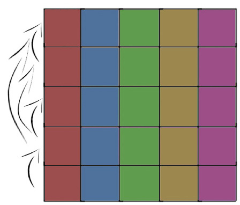
The blocked matrix data structure is ideally suited to carrying out each stage of MMF on a parallel system, because (except for summary statistics) no data needs to be communicated between the different blocks. However, changing the block structure of the matrix from one clustering to another can incur a large communication overhead. To retain m𝑚m–fold parallelism, the reblocking is carried out in two phases: first, each column of blocks is reblocked row-wise, then each row of blocks in the resulting new blocked matrix is reblocked column-wise (Figure 1).
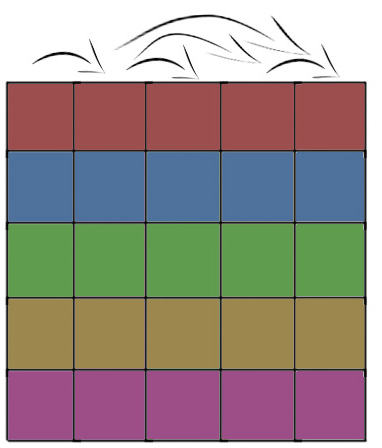
M11\!\!\!\left\llbracket M\right\rrbracket_{11}^{\phantom{M^{M}}} M12\!\!\!\left\llbracket M\right\rrbracket_{12} M13\!\!\!\left\llbracket M\right\rrbracket_{13} M14\!\!\!\left\llbracket M\right\rrbracket_{14} M15\!\!\!\left\llbracket M\right\rrbracket_{15}
M21\!\!\!\left\llbracket M\right\rrbracket_{21}^{\phantom{M^{M}}} M22\!\!\!\left\llbracket M\right\rrbracket_{22} M23\!\!\!\left\llbracket M\right\rrbracket_{23} M24\!\!\!\left\llbracket M\right\rrbracket_{24} M25\!\!\!\left\llbracket M\right\rrbracket_{25}
M31\!\!\!\left\llbracket M\right\rrbracket_{31}^{\phantom{M^{M}}} M32\!\!\!\left\llbracket M\right\rrbracket_{32} M33\!\!\!\left\llbracket M\right\rrbracket_{33} M34\!\!\!\left\llbracket M\right\rrbracket_{34} M35\!\!\!\left\llbracket M\right\rrbracket_{35}
M41\!\!\!\left\llbracket M\right\rrbracket_{41}^{\phantom{M^{M}}} M42\!\!\!\left\llbracket M\right\rrbracket_{42} M43\!\!\!\left\llbracket M\right\rrbracket_{43} M44\!\!\!\left\llbracket M\right\rrbracket_{44} M45\!\!\!\left\llbracket M\right\rrbracket_{45}
M51\!\!\!\left\llbracket M\right\rrbracket_{51}^{\phantom{M^{M}}} M52\!\!\!\left\llbracket M\right\rrbracket_{52} M53\!\!\!\left\llbracket M\right\rrbracket_{53} M54\!\!\!\left\llbracket M\right\rrbracket_{54} M55\!\!\!\left\llbracket M\right\rrbracket_{55}

Refer to caption

Refer to caption

Figure 1: Schematic of a blocked matrix M𝑀M with 5×5555\times 5 blocks. For the sake of visual clarity, we assumed that the blocks are contiguous, but, in general, this is not the case. The reblocking process involves first reorganizing the rows acoording to the new structure, then reorganizing the columns. To perform this efficiently, the first operation is done in parallel for each column of blocks of the original matrix, and the second operation is done in parallel for each row of blocks.

2.4 Sparsity and matrix-free MMF arithmetic

Ultimately, pMMF is intended for factoring matrices that are sparse, but whose dimensionality is in the hundreds of thousands or millions. As the factorization progresses, the fill-in (fraction of non-zeros) in Apsubscript𝐴𝑝A_{p} will increase, but at the same time, the active part of Asubscript𝐴A_{\ell} will progressively shrink. This means that in practice, given a sufficiently highly parallel system, the overall complexity can still scale roughly linearly with the number of non-zeros in A𝐴A.

The complete factorization appearing on the r.h.s. of (1) we denote A~~𝐴\tilde{A}. Storing A~~𝐴\tilde{A} by storing H𝐻H and the {Q}subscript𝑄\left\{Q_{\ell}\right\} matrices separately, the space complexity scales roughly linearly in the dimension. On the other hand, computing A~~𝐴\tilde{A} explicitly as a dense n×nsuperscript𝑛𝑛\mathbb{R}^{n\times n} matrix is usually unfeasible. Therefore, when applying the computed factorization, for example, as a preconditioner (Section 4), which requires repeatedly multilying a vector v𝑣v by A~~𝐴\tilde{A}, we use the so-called matrix-free approach: v𝑣v is stored in the same blocked form as A𝐴A, the rotations are applied individually, and as the different stages are applied to v𝑣v, the vector goes through an analogous reblocking process to that described for A𝐴A. The complexity of matrix-free MMF/vector multiplication is O(kpn)𝑂𝑘𝑝𝑛O(kpn). Inverting A~~𝐴\tilde{A}, which is also critical for downstream applications, involves inverting the entries on the diagonal of H𝐻H and inverting the core matrix, thus the overall complexity of MMF inversion is O(n+δL3)𝑂𝑛superscriptsubscript𝛿𝐿3O(n+\delta_{L}^{3}).

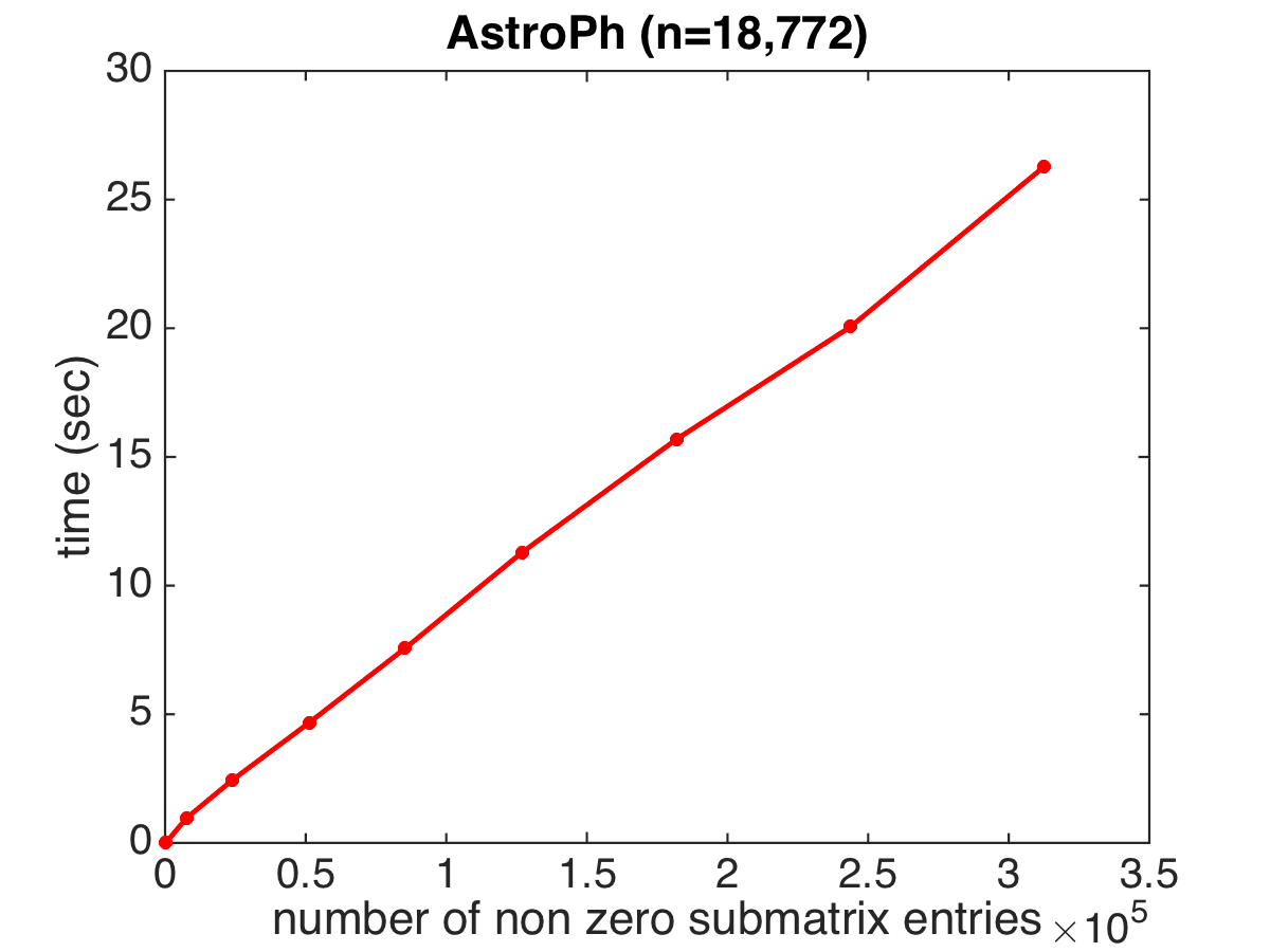
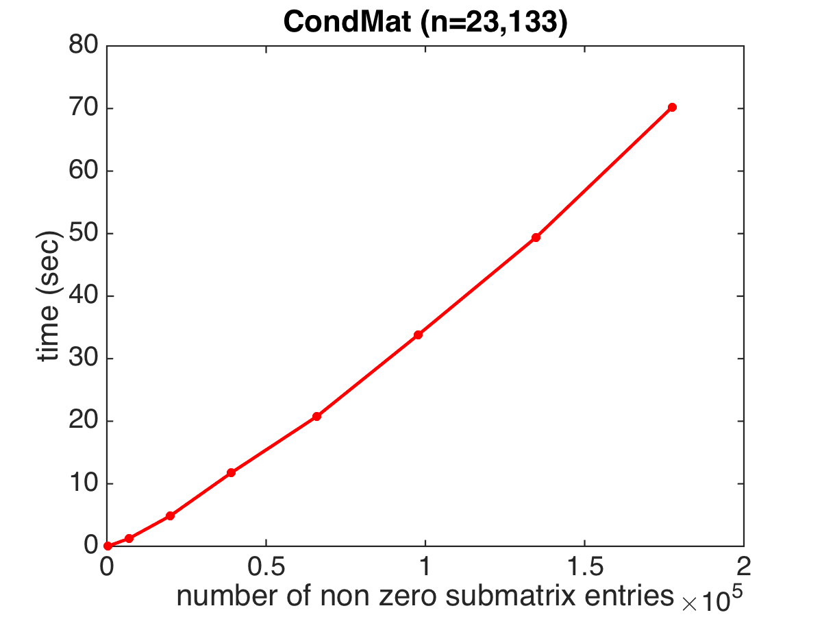
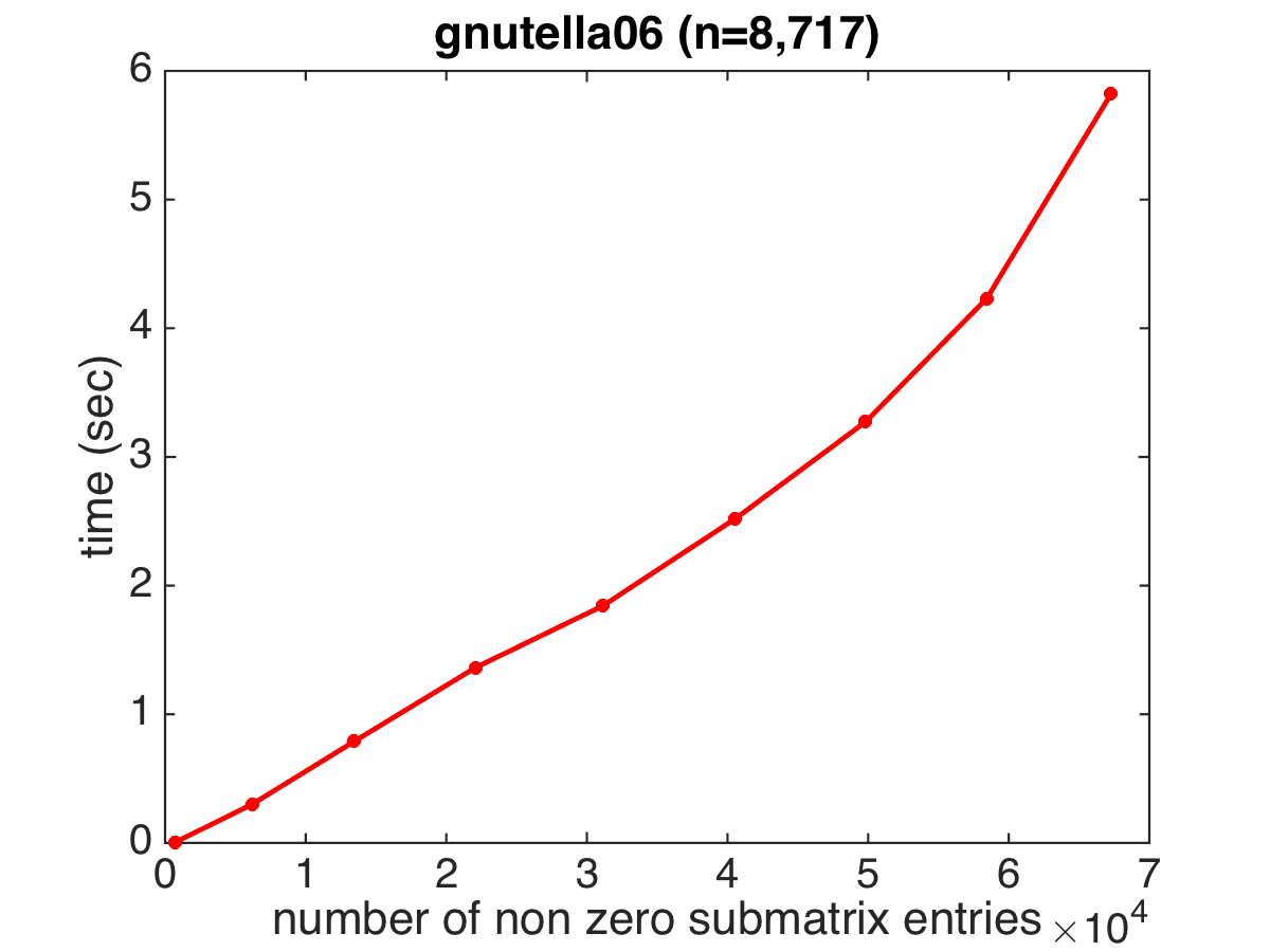
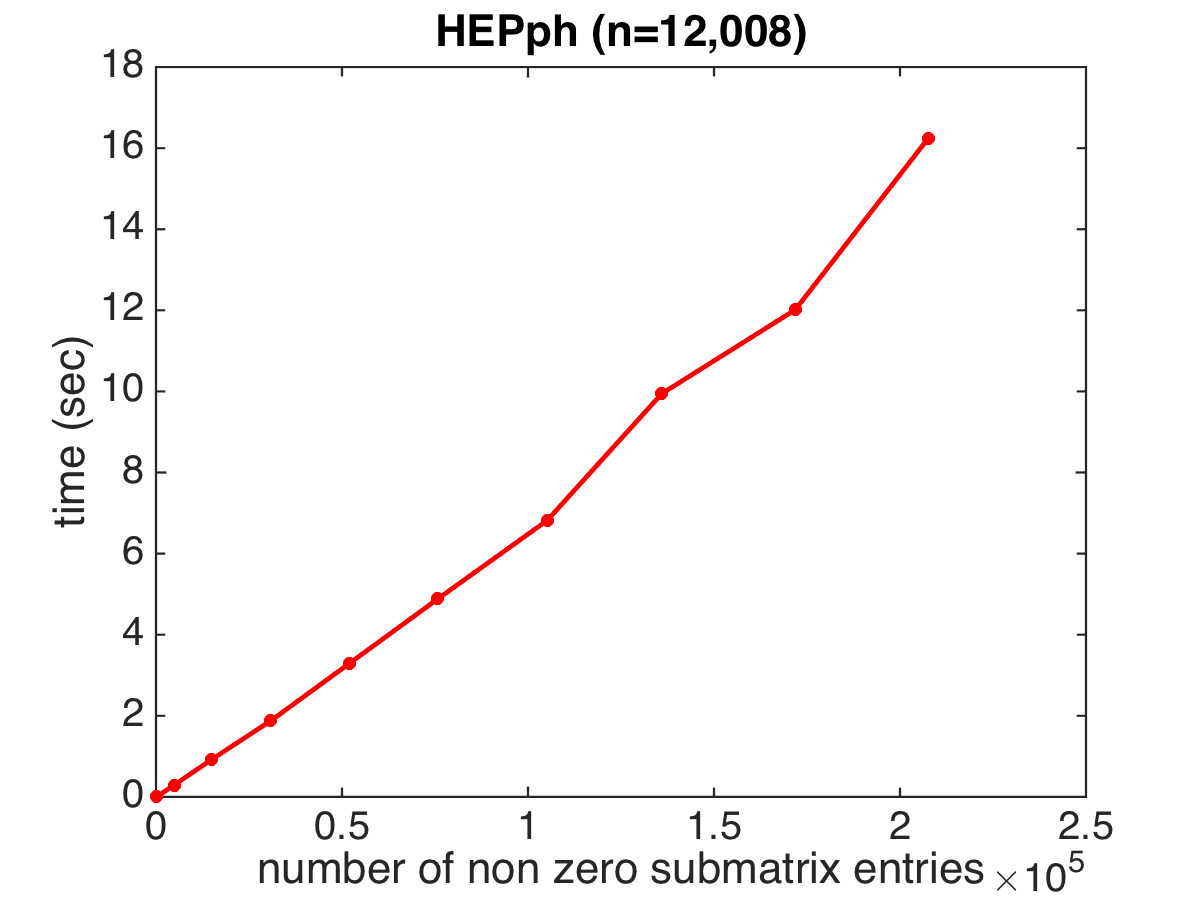
The theoretical complexity of the main components of pMMF are summarized in Table 1. Of course, requiring m2superscript𝑚2m^{2}–fold parallelism as m𝑚m\to\infty is an abstraction. Note, however, that even the total operation count scales with γn2𝛾superscript𝑛2\gamma n^{2}, which is just the number of non-zeros in the original matrix. The plots in Figure 2 and similar plots in the Supplement confirm that on many real world datasets, particularly, matrices coming from sparse network graphs, the wall clock time of pMMF tends to scale linearly with the dimension. Also note that in these experiments n𝑛n is on the order of 104105similar-tosuperscript104superscript10510^{4}\sim 10^{5}, yet the factorization time is on the order of just one minute.
Refer to caption
Refer to caption
Refer to caption
Refer to caption
Figure 2: Wall clock time of pMMF in seconds as a function of the number of non-zeros, γn2𝛾superscript𝑛2\gamma n^{2}, in A𝐴A on a 32 core 2.6 GHz machine. A𝐴A is derived from the Laplacian of standard benchmark sparse graphs (see Supplement), taking submatrices of different sizes. The figures confirm that in practice pMMF often scales linearly in the number of nonzeros, hence, for bounded degree graphs, also in n𝑛n.

3 pMMF Compression

Most, if not all, machine learning algorithms reduce to linear algebra operations or optimization over large instance/feature matrices or instance/instance similarity matrices. The classical example is, of course, kernel methods, which reduce to convex optimization involving the so-called Gram matrix, a symmetric positive semi-definite (p.s.d.) matrix of size n×n𝑛𝑛n\times n, where n𝑛n is the number of training examples. Despite their many attractive properties and their large literature, the applicability of kernel methods to today’s large datasets is limited by the fact that “out of the box” their computation time scales with about n3superscript𝑛3n^{3}. This issue (not just for kernel methods, but more broadly) has catalyzed an entire area focused on compressing or “sketching” matrices with minimal loss.

In the symmetric (and p.s.d) case, most sketching algorithms approximate An×n𝐴superscript𝑛𝑛A\in\mathbb{R}^{n\times n} in the form A~=CWC~𝐴𝐶superscript𝑊superscript𝐶top\tilde{A}=CW^{\dagger}C^{\top}, where C𝐶C is a judiciously chosen n×msuperscript𝑛𝑚\mathbb{R}^{n\times m} matrix with mnmuch-less-than𝑚𝑛m\ll n, and Wsuperscript𝑊W^{\dagger} is computed by taking the pseudo-inverse of a certain matrix that is of size only m×m𝑚𝑚m\times m. The algorithms mainly differ in how they define C𝐶C:

  1. (i)

    Projection based methods set each column of C𝐶C to be a random linear combination of the columns of the original matrix A𝐴A, and use Johnson–Lindenstrauss type arguments to show that the resulting low dimensional random sketch preserves most of the information at least about the part of A𝐴A spanned by its high eigenvalue eigenvectors [8]. These methods come with strong guarantees, but suffer from the cost of having to compute m𝑚m dense linear combinations of the columns of A𝐴A. Even if A𝐴A was sparse, this process destroys the sparsity.

  2. (ii)

    Structured projections are a twist on the above idea, replacing the random projection with a fixed, dense, but efficiently computable, basis transformation (and subsampling in that basis), such as the fast Hadamard transform or the fast Fourier transform [9, 10].

  3. (iii)

    In contrast to (i) and (ii), Nyström algorithms construct C𝐶C by choosing a certain number of actual columns of A𝐴A, usually by random sampling. Here, the focus has shifted from uniform sampling [11, 12], via l2subscript𝑙2l_{2}–norm sampling [13], to sampling based on so-called leverage scores [14, 15, 16], which, for low rank matrices, can be shown to be optimal. Further recent developments include the ensemble Nyström method [17] and the clustered Nyström algorithm [18]. Finally, a number of adaptive algorithms have also been proposed [19, 20, 21].

pMMF can also be regarded as a sketching method, in the sense that (2) compresses A𝐴A into an m:=δLnassign𝑚subscript𝛿𝐿much-less-than𝑛m\!:=\!\delta_{L}\ll n dimensional core via a very fast series of orthogonal transforms QLQ2Q1subscript𝑄𝐿subscript𝑄2subscript𝑄1Q_{L}\ldots Q_{2}Q_{1}, which play a role analogous to Csuperscript𝐶topC^{\top}​​. In contrast to the other methods, however, MMF also retains the entries on the diagonal of H𝐻H. From the point of view of downstream computation, this incurs very little extra cost. For example, if the purpose of sketching A𝐴A is to compute its inverse, maybe for use in a Gaussian process or ridge regression, then A~1superscript~𝐴1\tilde{A}^{-1} can be easily computed by inverting the core of H𝐻H (as in the Nyström methods), and just taking the inverse of all other matrix elements on the diagonal.
Refer to caption

Refer to caption

Refer to caption

Refer to caption

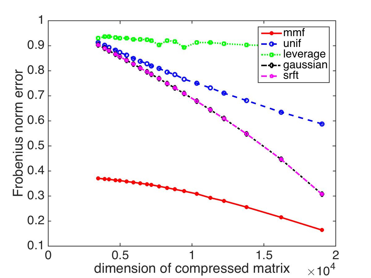
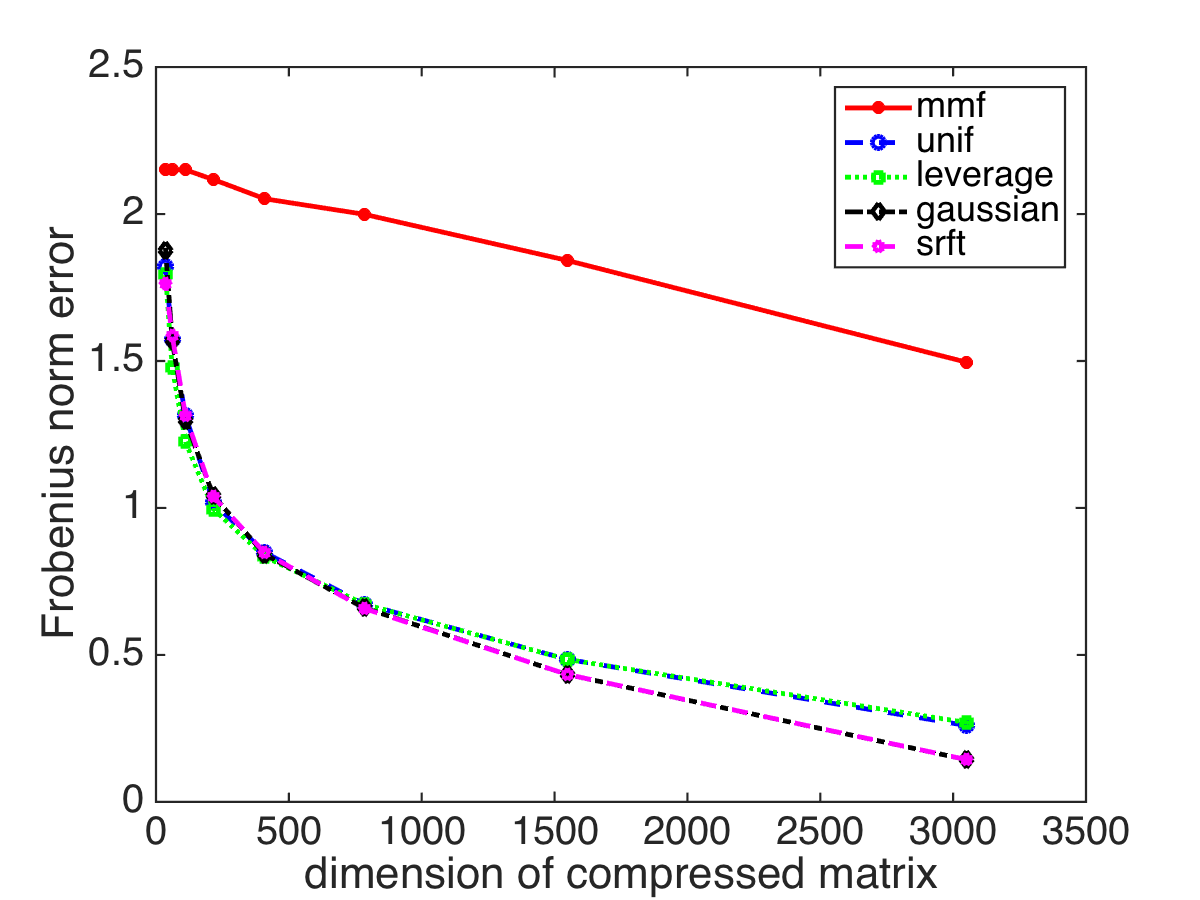
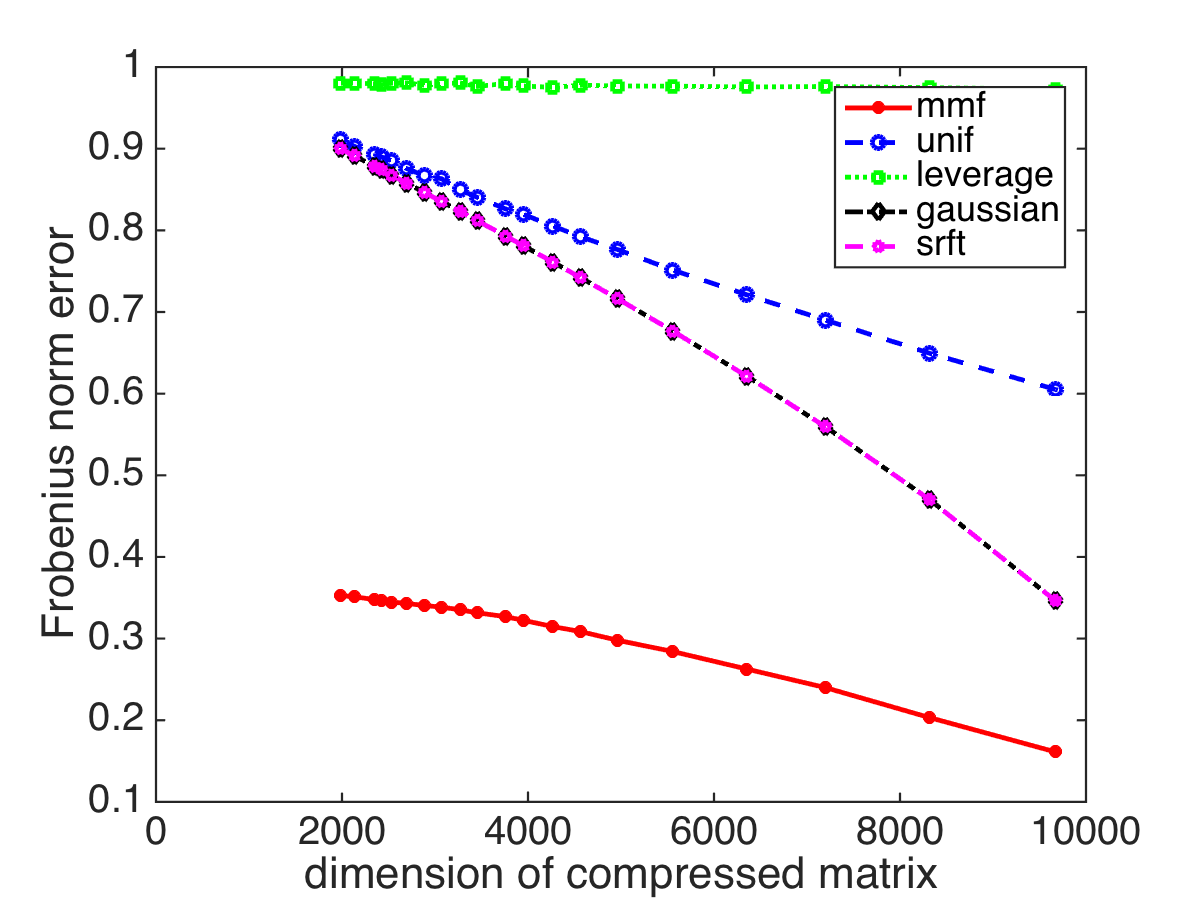
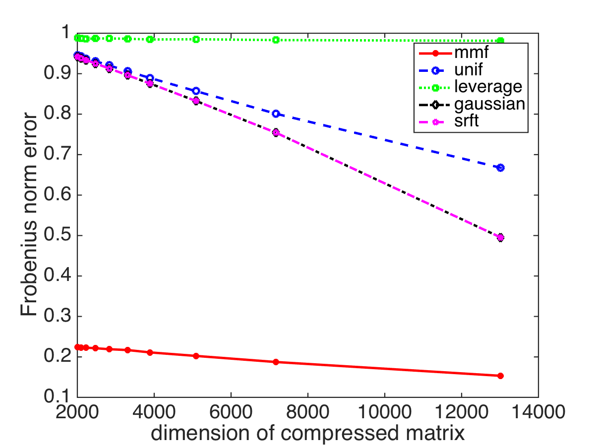
Figure 3: The Frobenius norm error AA~Frobsubscriptnorm𝐴~𝐴Frob\Arrowvert\,A-\tilde{A}\,\Arrowvert_{\text{Frob}} of compressing matrices with pMMF vs. other sketching methods, as a function of the dimension of the compressed core. In each figure, the error is normalized by AAkFrobsubscriptnorm𝐴subscript𝐴𝑘Frob\Arrowvert\,A-A_{k}\,\Arrowvert_{\text{Frob}}, where Aksubscript𝐴𝑘A_{k} is the best rank k𝑘k approximation to A𝐴A. The four datasets are “HEPph”, “AstroPh”, “CondMat” and “Gisette”, with k=100𝑘100k=100 in the first three and k=12𝑘12k=12 in “Gisette”.

The main distinction between pMMF and other matrix sketching methods is that while the latter, implicitly or explicitly, make the assumption that A𝐴A is low rank, or close to low rank, MMF makes a different structural assumption about A𝐴A, namely that it has hidden hierarchical or multiresolution structure. Figure 3 shows the results of experiments comparing the perfomance of MMF to other matrix sketching algorithms on some standard datasets. As in panes 1–3, on most datasets that we tried, pMMF significantly outperforms the other sketching methods in both Frobenius norm error and spectral norm error (plots of the latter can be found in the Supplement). The advantage of pMMF seems to be particularly great on network graphs, perhaps not surprisingly, since it has long been conjectured that networks have multiresolution structure [22, 23, 24]. However, we find that pMMF often outperforms other methods on kernel matrices in general. On the other hand, on a small fraction of datasets, typically those which explicitly have low rank or are very close to being low rank (e.g., the fourth pane of Figure 3), pMMF performs much worse than expected. In such cases, a combination of the low rank and multiresolution approaches might be most advantageous, which is the subject of ongoing work.

It is important to emphasize that pMMF is very scalable. Many other Nyström methods are implemented in MATLAB, which limits the size of datasets on which they can be feasibly ran on. Moreover, leverage score methods require estimating the singular vectors of A𝐴A, which, unless A𝐴A is very low rank, can be a computational bottleneck. Several of the Nyström experiments took 30 minutes or more to run on 8 cores, whereas our custom C++ pMMF implementation compressed the matrix in at most one or two minutes (see more timing results in the Supplement). Hence, pMMF addresses a different regime than many other Nyström papers: whereas the latter often focus on compressing 103similar-toabsentsuperscript103\sim\!10^{3} dimensional matrices to just 10–100 dimensions, we are more interested in compressing 104similar-toabsentsuperscript104\sim\!10^{4}105superscript10510^{5} dimensional matrices to 103similar-toabsentsuperscript103\sim\!10^{3} dimensions.

4 pMMF Preconditioning

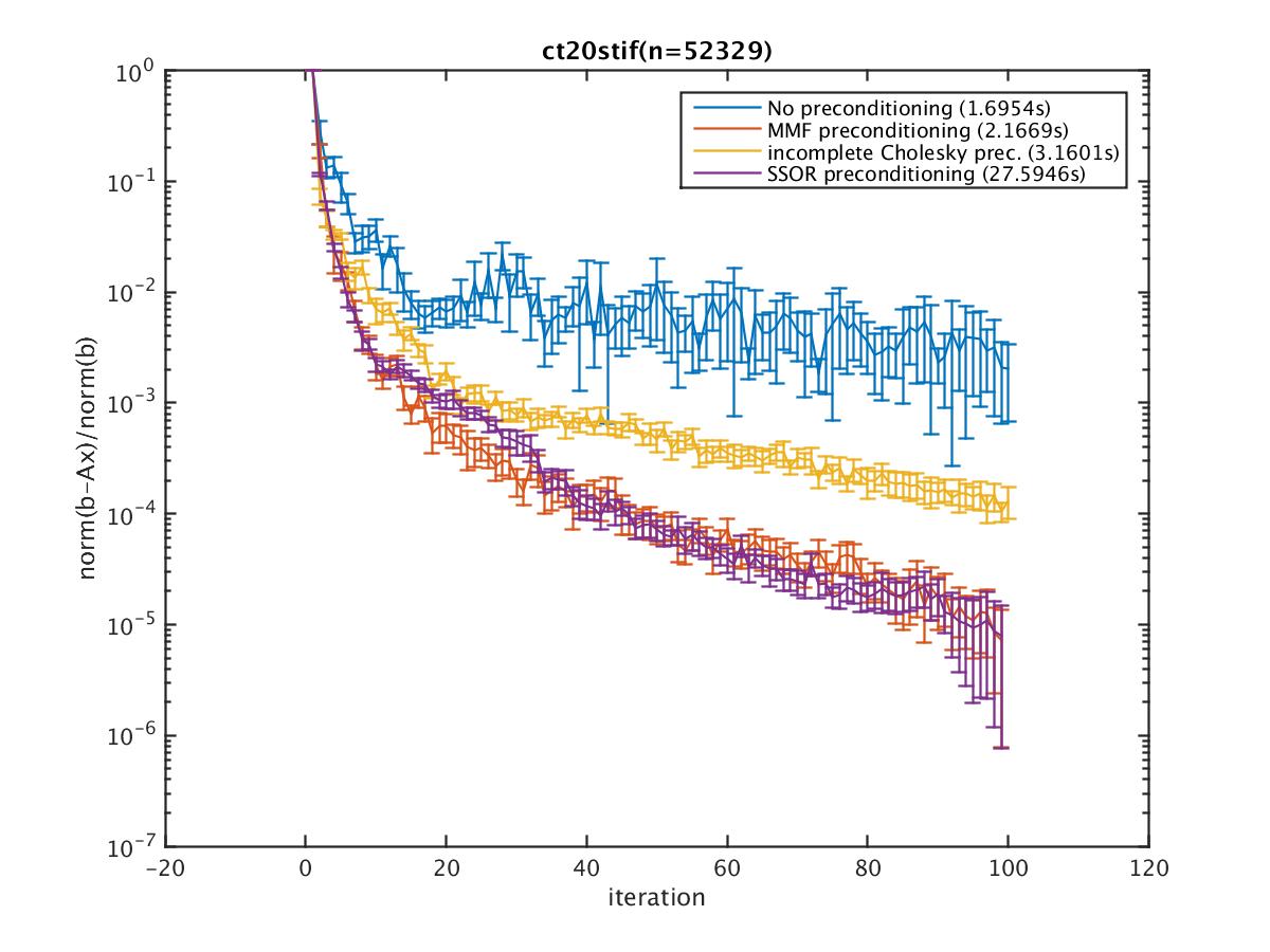
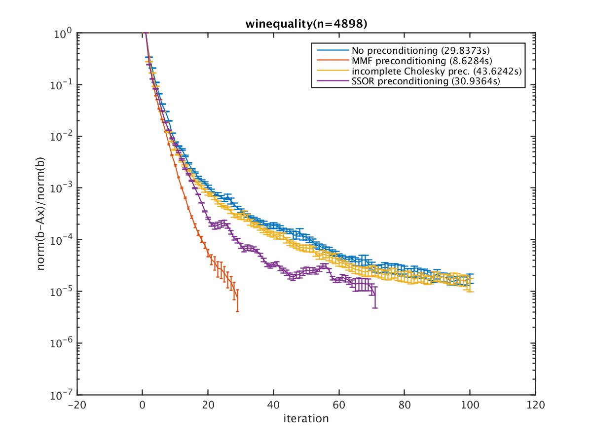
Given a large matrix An×n𝐴superscript𝑛𝑛A\in\mathbb{R}^{n\times n}, and a vector bn𝑏superscript𝑛b\in\mathbb{R}^{n}, solving the linear system Ax=b𝐴𝑥𝑏Ax=b is one of the most fundamental problems in computational mathematics. In the learning context, solving linear systems is the computational bottleneck in a range of algorithms. When A𝐴A is sparse, Ax=b𝐴𝑥𝑏Ax=b is typically solved with iterative methods, such as conjugate gradients. However, it is well known that the number of iterations needed for such methods to converge scales badly with κ𝜅\kappa, where κ𝜅\kappa is the ratio of the largest and smallest eigenvalues of A𝐴A, called the condition number.

The idea of preconditioning is to solve instead of Ax=b𝐴𝑥𝑏Ax=b the related system (M1A)x=M1bsuperscript𝑀1𝐴𝑥superscript𝑀1𝑏(M^{-1}A)\hskip 1.11115ptx=M^{-1}b, where M1superscript𝑀1M^{-1} is an easy to compute rough approximation to A1superscript𝐴1A^{-1}. A good preconditioner will ensure that M1Asuperscript𝑀1𝐴M^{-1}A is fast to multiply with the current vector iterate, while the condition number of M1Asuperscript𝑀1𝐴M^{-1}A is much better than that of the original matrix A𝐴A. At the same time, it is important that M1superscript𝑀1M^{-1} be easily computable for massive matrices. For symmetric matrices, a variation on the above is to solve (M1/2AM1/2)y=M1/2bsuperscript𝑀12𝐴superscript𝑀12𝑦superscript𝑀12𝑏(M^{-1/2}A\hskip 0.55557ptM^{-1/2})\hskip 1.11115pty=M^{-1/2}\hskip 1.11115ptb, and then set x=M1/2y𝑥superscript𝑀12𝑦x=M^{-1/2}y, which retains symmetry. pMMF is a natural candidate preconditioner for symmetric matrices since (a) the pMMF factorization can be computed very fast (b) as evidenced by the previous section, A~~𝐴\tilde{A} is a good approximation to A𝐴A, (c) A~ξsuperscript~𝐴𝜉\tilde{A}^{-\xi} (with ξ{1,1/2}𝜉112\xi\in\{1,1/2\}) can be computed from A~~𝐴\tilde{A} in just O(n+δL3)𝑂𝑛superscriptsubscript𝛿𝐿3O(n+\delta_{L}^{3}) time. However, unlike some other preconditioners, A~ξsuperscript~𝐴𝜉\tilde{A}^{-\xi} is generally not sparse. Therefore, in MMF preconditioning one never expands A~ξsuperscript~𝐴𝜉\tilde{A}^{-\xi} into a full matrix, but rather A~ξsuperscript~𝐴𝜉\tilde{A}^{-\xi} is applied to the vectors involved in the iterative method of choice as a sequence of rotations, as described in Section 2.4.

A large number of different preconditioners have been proposed in the literature, and even for a given type of problem there is often no single best choice, rather the choice reduces to experimentation. In our experiments our goal was to show that pMMF preconditioning can improve the convergence of linear solvers in learning problems, and that it is competitive with other preconditioners. Figure 4 compares the performance of pMMF as a preconditioner to other standard preconditioners, such as incomplete Cholesky and SSOR. Several more preconditioning results are presented in the Supplement. In summary, pMMF appears competitive with other preconditioners on network and kernel matrices, and sometimes outperforms other methods. In each of our experiments, the time required to compute the pMMF preconditioner was less than a minute, which is amortized over the number of linear solves. We are still experimenting with how much pMMF as a preconditioner can be improved by fine tuning its parameters, and how well it will perform coupled with other solvers.
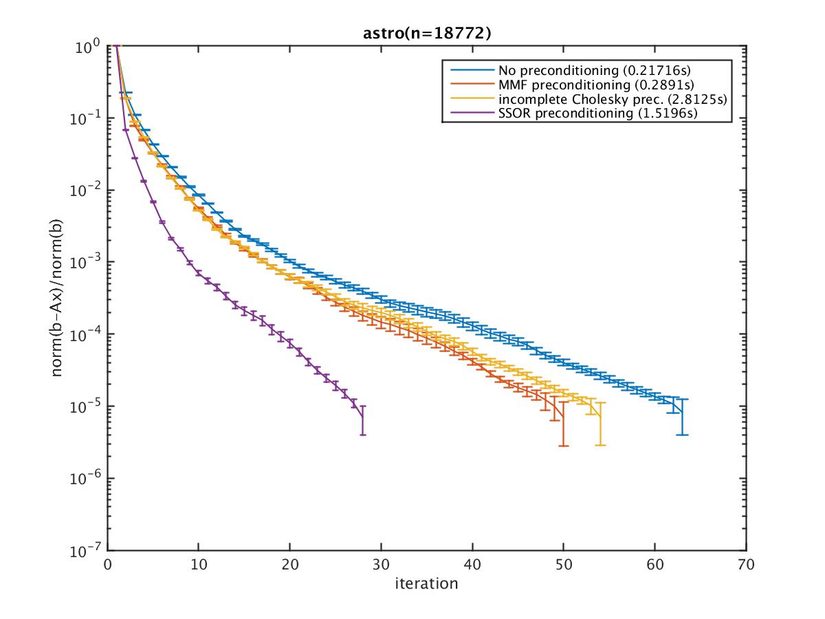
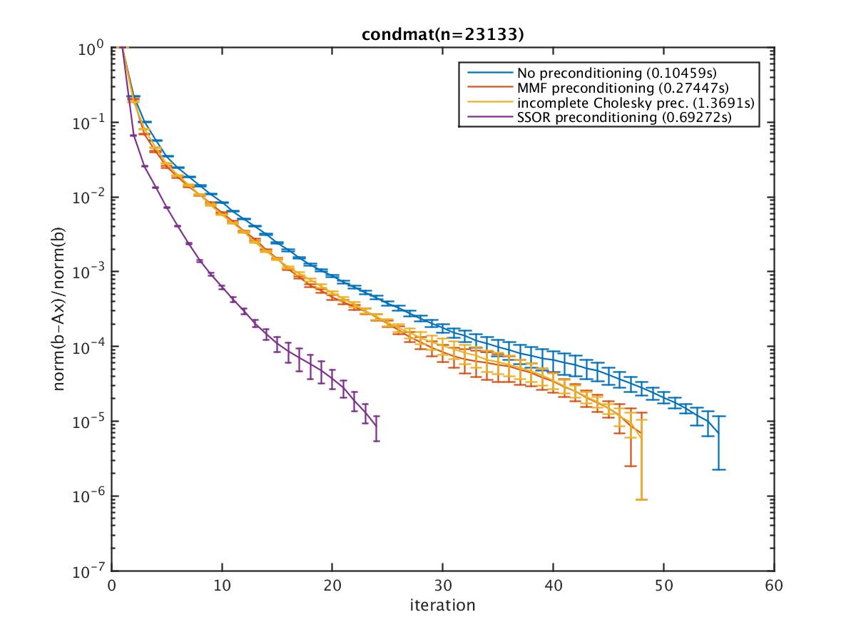
Refer to caption

Refer to caption

Refer to caption

Refer to caption

Figure 4: Residual as a function of conjugate gradient iterations when solving Ax=b𝐴𝑥𝑏Ax=b, where b𝑏b is a dense random vector. The indicated times are the wall clock time to convergence on an 8 core 2.62.62.6 GHz machine. The per-iteration time of pMMF preconditioning is usually 2–10 times faster than of other methods. pMMF is indicated in red.

5 Conclusions

The most common structural assumption about large matrices arising in learning problems is that they are low rank. This paper explores the alternative approach of assuming that they have multiresolution structure. Our results suggest that not only is the multiresolution model often more faithful to the actual structure of data (e.g., as evidenced by much lower approximation error in compression experiments), but it also lends itself to devising efficient parallel algorithms, which is critical to dealing with large scale problems. Our approach bears some similarities to multigrid methods [26] and structured matrix decompositions [27, 28, 29], which are extremely popular in applied mathematics, primarily in the context of solving systems of partial differential equations. A crucial difference, however, is that whereas in these algorithms the multiresolution structure is suggested by the geometry of the domain, in learning problems the structure itself has to be learnt “on the fly”. Empirically, the pMMF algorithm described in this paper scales linearly in the size of the data. Further work will explore folding entire learning and optimization algorithms into the multiresolution framework, while retaining the same scaling behavior.

serial MMF pMMF operations pMMF time dense sparse dense sparse dense sparse Nprocsubscript𝑁procN_{\text{proc}} Computing Grams O(n3)𝑂superscript𝑛3O(n^{3}) O(γn3)𝑂𝛾superscript𝑛3O(\gamma n^{3}) O(pcn2)𝑂𝑝𝑐superscript𝑛2O(pcn^{2}) O(γpcn2)𝑂𝛾𝑝𝑐superscript𝑛2O(\gamma pcn^{2}) O(pc3)𝑂𝑝superscript𝑐3O(pc^{3}) O(γpc3)𝑂𝛾𝑝superscript𝑐3O(\gamma pc^{3}) m2superscript𝑚2m^{2} Finding Rotations O(n3)𝑂superscript𝑛3O(n^{3}) O(n3)𝑂superscript𝑛3O(n^{3}) O(cn)𝑂𝑐𝑛O(cn) O(cn)𝑂𝑐𝑛O(cn) O(c2)𝑂superscript𝑐2O(c^{2}) O(c2)𝑂superscript𝑐2O(c^{2}) msuperscript𝑚absentm^{\phantom{2}} Updating Grams O(n3)𝑂superscript𝑛3O(n^{3}) O(γ2n3)𝑂superscript𝛾2superscript𝑛3O(\gamma^{2}n^{3}) O(c2n)𝑂superscript𝑐2𝑛O(c^{2}n) O(γ2c2n)𝑂superscript𝛾2superscript𝑐2𝑛O(\gamma^{2}c^{2}n) O(c3)𝑂superscript𝑐3O(c^{3}) O(γ2c3)𝑂superscript𝛾2superscript𝑐3O(\gamma^{2}c^{3}) msuperscript𝑚absentm^{\phantom{2}} Applying rotations O(kn2)𝑂𝑘superscript𝑛2O(kn^{2}) O(γkn2)𝑂𝛾𝑘superscript𝑛2O(\gamma kn^{2}) O(kn2)𝑂𝑘superscript𝑛2O(kn^{2}) O(γkn2)𝑂𝛾𝑘superscript𝑛2O(\gamma kn^{2}) O(kc2)𝑂𝑘superscript𝑐2O(kc^{2}) O(γkc2)𝑂𝛾𝑘superscript𝑐2O(\gamma kc^{2}) m2superscript𝑚2m^{2} Clustering O(pmn2)𝑂𝑝𝑚superscript𝑛2O(pmn^{2}) O(γpmn2)𝑂𝛾𝑝𝑚superscript𝑛2O(\gamma pmn^{2}) O(pcn)𝑂𝑝𝑐𝑛O(pcn) O(γpcn)𝑂𝛾𝑝𝑐𝑛O(\gamma pcn) m2superscript𝑚2m^{2} Reblocking O(pn2)𝑂𝑝superscript𝑛2O(pn^{2}) O(γpn2)𝑂𝛾𝑝superscript𝑛2O(\gamma pn^{2}) O(pcn)𝑂𝑝𝑐𝑛O(pcn) O(γpcn)𝑂𝛾𝑝𝑐𝑛O(\gamma pcn) msuperscript𝑚absentm^{\phantom{2}} Factorization total O(n3)𝑂superscript𝑛3O(n^{3}) O(n3)𝑂superscript𝑛3O(n^{3}) O(pcn2)𝑂𝑝𝑐superscript𝑛2O(pcn^{2}) O(γpcn2)𝑂𝛾𝑝𝑐superscript𝑛2O(\gamma pcn^{2}) O(pc3)𝑂𝑝superscript𝑐3O(pc^{3}) O(γpc3)𝑂𝛾𝑝superscript𝑐3O(\gamma pc^{3}) m2superscript𝑚2m^{2}

Table 1: The rough complexity of different subtasks in pMMF vs. in the original serial MMF algorithm of [4]. Here n𝑛n is the dimensionality of the original matrix, A𝐴A, k𝑘k is the order of the rotations, and γ𝛾\gamma is the fraction of non-zero entries in A𝐴A, when A𝐴A is sparse. We neglect that during the course of the computation γ𝛾\gamma tends to increase, because concomitantly Asubscript𝐴A_{\ell} shrinks, and computation time is usually dominated by the first few stages. We also assume that entries of sparse matrices can be accessed in constant time. In pMMF, p𝑝p is the number of stages, m𝑚m is the number of clusters in each stage, and c𝑐c is the typical cluster size (thus, c=θ(n/m)𝑐𝜃𝑛𝑚c=\theta(n/m)). The “pMMF time” columns give the time complexity of the algorithm assuming an architecture that affords Nprocsubscript𝑁procN_{\text{proc}}–fold parallelism. g=δL𝑔subscript𝛿𝐿g=\delta_{L} is the size of the dense core in H𝐻H. It is assumed that kpcn𝑘𝑝𝑐𝑛k\leq p\leq c\leq n, but n=o(c2)𝑛𝑜superscript𝑐2n=o(c^{2}).

References

  • [1] Qirong Ho, James Cipar, Henggang Cui, Seunghak Lee, Jin Kyu Kim, Phillip B Gibbons, Garth A Gibson, Greg Ganger, and Eric P Xing. More effective distributed ml via a stale synchronous parallel parameter server. In Advances in neural information processing systems, pages 1223–1231, 2013.
  • [2] Mu Li, Li Zhou, Zichao Yang, Aaron Li, Fei Xia, David G Andersen, and AJ Smola. Parameter server for distributed machine learning. In Big Learning NIPS Workshop, 2013.
  • [3] Seunghak Lee, Jin Kyu Kim, Xun Zheng, Qirong Ho, Garth A Gibson, and Eric P Xing. On model parallelization and scheduling strategies for distributed machine learning. In Advances in Neural Information Processing Systems, pages 2834–2842, 2014.
  • [4] Risi Kondor, Nedelina Teneva, and Vikas Garg. Multiresolution Matrix Factorization. In Proceedings of the 31st International Conference on Machine Learning (ICML-14), pages 1620–1628, 2014.
  • [5] Ronald R. Coifman, Ronald R Coifman, and Mauro Maggioni. Multiresolution analysis associated to diffusion semigroups: construction and fast algorithms. 2004.
  • [6] Ann B Lee, Boaz Nadler, and Larry Wasserman. Treelets — An adaptive multi-scale basis for sparse unordered data. Annals of Applied Statistics, 2(2):435–471, 2008.
  • [7] Aydin Buluç and John R Gilbert. Parallel sparse matrix-matrix multiplication and indexing: implementation and experiments. SIAM J Sci Comput, 34(4), 2012.
  • [8] Nathan Halko, Per-Gunnar Martinsson, and Joel A Tropp. Finding structure with randomness: Probabilistic algorithms for constructing approximate matrix decompositions. SIAM review, 53(2):217–288, 2011.
  • [9] Nir Ailon and Bernard Chazelle. The Fast Johnson–Lindenstrauss Transform and Approximate Nearest Neighbors. SIAM Journal on Computing, 39(1):302–322, January 2009.
  • [10] Quoc Le, Tamás Sarlós, and Alexander Smola. Fastfood: – computing Hilbert space expansions in loglinear time. JMLR, 2013.
  • [11] C. Williams and M. Seeger. Using the Nyström method to speed up kernel machines. In Advances in Neural Information Processing Systems (NIPS), 2001.
  • [12] Charless Fowlkes, Serge Belongie, Fan Chung, and Jitendra Malik. Spectral grouping using the Nyström method. IEEE transactions on pattern analysis and machine intelligence, 26(2):214–25, February 2004.
  • [13] P. Drineas, R. Kannan, and M. W. Mahoney. Fast monte carlo algorithms for matrices I–III. SIAM Journal on Computing, 36(1):158–183, 2006.
  • [14] Michael W Mahoney and Petros Drineas. CUR matrix decompositions for improved data analysis. Proceedings of the National Academy of Sciences, 106(3):697–702, 2009.
  • [15] M. W. Mahoney. Randomized algorithms for matrices and data. Foundations and Trends in Machine Learning, 3, 2011.
  • [16] Alex Gittens and Michael W Mahoney. Revisiting the Nyström method for improved large-scale machine learning. volume 28, 2013.
  • [17] Sanjiv Kumar, Mehryar Mohri, and Ameet Talwalkar. Ensemble Nyström Method. 2009.
  • [18] Kai Zhang and James T Kwok. Clustered Nyström method for large scale manifold learning and dimension reduction. IEEE transactions on neural networks / a publication of the IEEE Neural Networks Council, 21(10):1576–87, October 2010.
  • [19] Amit Deshpande, Luis Rademacher, Santosh Vempala, and Grant Wang. Matrix approximation and projective clustering via volume sampling. In Proceedings of the seventeenth annual ACM-SIAM symposium on Discrete algorithm, pages 1117–1126. ACM, 2006.
  • [20] Sanjiv Kumar, Mehryar Mohri, and Ameet Talwalkar. Sampling Methods for the Nyström method. Journal of Machine Learning Research, 13:981–1006, 2012.
  • [21] Shusen Wang and Zhihua Zhang. Improving CUR Matrix Decomposition and the Nyström Approximation via Adaptive Sampling. 14:2729–2769, 2013.
  • [22] Erzsébet Ravasz and Albert-László Barabási. Hierarchical organization in complex networks. Physical Review E, 67(2):026112, February 2003.
  • [23] R R Coifman and M Maggioni. Diffusion wavelets. Applied and Computational Harmonic Analysis, 2006.
  • [24] Berkant Savas, Inderjit S Dhillon, et al. Clustered low rank approximation of graphs in information science applications. In SDM, pages 164–175. SIAM, 2011.
  • [25] The GNU Public License, Version 3, http://www.gnu.org/licenses/.
  • [26] Achi Brandt. Multi-level adaptive technique (mlat) for fast numerical solution to boundary value problems. In Henri Cabannes and Roger Temam, editors, Proceedings of the Third International Conference on Numerical Methods in Fluid Mechanics, volume 18 of Lecture Notes in Physics, pages 82–89. Springer Berlin Heidelberg, 1973.
  • [27] Wolfgang Hackbusch. A Sparse Matrix Arithmetic based on H -Matrices . Part I : Introduction to H -Matrices . 62:1–12, 1999.
  • [28] Steffen Borm. Construction of data-sparse H2superscript𝐻2H^{2}-matrices by hierarchical compression. pages 1–33, 2007.
  • [29] S. Chandrasekaran, M. Gu, and W. Lyons. A fast adaptive solver for hierarchically semiseparable representations. Calcolo, 42(3-4):171–185, 2005.