Bayesian global analysis of neutrino oscillation data

Abstract

We perform a Bayesian analysis of current neutrino oscillation data. When estimating the oscillation parameters we find that the results generally agree with those of the $\chi^{2}$ method, with some differences involving $s^{2}_{23}$ and CP-violating effects. We discuss the additional subtleties caused by the circular nature of the CP-violating phase, and how it is possible to obtain correlation coefficients with $s^{2}_{23}$. When performing model comparison, we find that there is no significant evidence for any mass ordering, any octant of $s^{2}_{23}$ or a deviation from maximal mixing, nor the presence of CP-violation

1 Introduction

Neutrino oscillation experiments have now established beyond doubt that neutrinos are massive and there is leptonic flavour violation in their propagation  Pontecorvo:1967fh ; Gribov:1968kq , see Ref. GonzalezGarcia:2007ib for an overview. It has also been clear for more than a decade that a consistent description of the global data on neutrino oscillations is possible by assuming that the three known neutrinos ($\nu_{e}$, $\nu_{\mu}$, $\nu_{\tau}$) are linear quantum superposition of three massive states $\nu_{i}$ ($i=1,2,3$) with masses $m_{i}$. Consequently, a leptonic mixing matrix is present in the weak charged current interactions Maki:1962mu ; Kobayashi:1973fv of the mass eigenstates, which can be parametrized as PDG :

$$U=\begin{pmatrix}c_{12}c_{13}&s_{12}c_{13}&s_{13}e^{-i\delta_{\text{CP}}}\\ -s_{12}c_{23}-c_{12}s_{13}s_{23}e^{i\delta_{\text{CP}}}&\hphantom{+}c_{12}c_{23}-s_{12}s_{13}s_{23}e^{i\delta_{\text{CP}}}&c_{13}s_{23}\\ \hphantom{+}s_{12}s_{23}-c_{12}s_{13}c_{23}e^{i\delta_{\text{CP}}}&-c_{12}s_{23}-s_{12}s_{13}c_{23}e^{i\delta_{\text{CP}}}&c_{13}c_{23}\end{pmatrix},$$ (1)

where $c_{ij}\equiv\cos\theta_{ij}$ and $s_{ij}\equiv\sin\theta_{ij}$. If one chooses the convention where the angles $\theta_{ij}$ are taken to lie in the first quadrant, $\theta_{ij}\in[0,\pi/2]$, and the CP phase $\delta_{\text{CP}}\in[0,2\pi]$, then $\Delta m^{2}_{21}=m_{2}^{2}-m_{1}^{2}>0$ by convention, and $\Delta m^{2}_{31}$ can be positive or negative. It is customary to refer to the first option as Normal Ordering (NO), and to the second one as Inverted Ordering (IO). In the following we adopt the (arbitrary) convention of reporting results for $\Delta m^{2}_{31}$ for NO and $\Delta m^{2}_{32}$ for IO, i.e., we always use the one which has the larger absolute value. Sometimes we will generically denote such quantity as $\Delta m^{2}_{3\ell}$, with $\ell=1$ for NO and $\ell=2$ for IO.

Several global analyses exist in the literature Gonzalez-Garcia:2014bfa ; Capozzi:2013csa ; Forero:2014bxa , which, by fitting the results from the bulk of oscillation experiments, obtain best estimates and allowed ranges for these six oscillation parameters. Generically they obtain their results within a frequentist framework, using a $\chi^{2}$ statistics.

Alternatively, a consistent approach to obtaining the probability that a certain parameter within a given model takes certain values is provided by Bayesian inference. Furthermore, Bayesian analysis is particularly suited for comparing how much better one model describes the data compared to another model. So one may question to what degree the current determination of the oscillation parameters is dependent on the assumed statistical approach, and whether Bayesian statistics can shed some light on the presently open issues related to the mass ordering, the octant of $\theta_{23}$, and the presence of CP-violation.

In this article we address these questions by performing a Bayesian analysis of the current neutrino oscillation data. In Sec. 2 we briefly describe the elements of Bayesian statistics required for this analysis. In Sec. 3 we present the global results of the analysis and compare them with those of the $\chi^{2}$ analysis of the same data samples of NuFIT 2.0 nufit . We discuss in detail the main results related to the determination of $\sin^{2}\theta_{23}$ and $\delta_{\rm CP}$ in Secs. 4 and 5, where we also discuss the additional subtleties caused by the circular nature of the CP-violating phase, and study how it is possible to define correlation coefficients with $s^{2}_{23}$ in Sec. 6. Finally in Sec. 7 we summarize our conclusions.

2 Statistical framework

In this work, we will be using Bayesian probability theory, where each proposition is associated with a probability or plausibility, defined to lie between 0 and 1. In order to calculate the probabilities of different assumptions, hypotheses, or models, the laws of probability are used when conditioned on some known (or assumed) information. Of particular interest is Bayes’ theorem, which can be used to compare a set of hypotheses $M_{j}$, using some set of collected data, $\mathbf{D}$, through calculation of the posterior odds,

$$\frac{\Pr(M_{i}|\mathbf{D})}{\Pr(M_{j}|\mathbf{D})}=\frac{\Pr(\mathbf{D}|M_{i})}{\Pr(\mathbf{D}|M_{j})}\frac{\Pr(M_{i})}{\Pr(M_{j})}.$$ (2)

The prior odds $\Pr(M_{i})/\Pr(M_{j})$ quantifies how much more plausible one model is than the other a priori. The evidence, $\mathcal{Z}_{i}=\Pr(\mathbf{D}|M_{i})$, is the likelihood for the model quantifying how well the model describes the data. The Bayes factor,

$$\mathcal{B}=\mathcal{Z}_{i}/\mathcal{Z}_{j}$$ (3)

which is the ratio of the evidences, quantifies how much better the model $M_{i}$ describes the data than $M_{j}$.

Given that the model $M$ contains the free parameters $\mathbf{\Theta}$, the evidence is given by

$$\mathcal{Z}=\Pr(\mathbf{D}|M) = \int{\mathcal{L}(\mathbf{\Theta})\pi(\mathbf{\Theta})}{\rm d}^{N}\mathbf{\Theta},$$ (4)

where $\mathcal{L}(\mathbf{\Theta})\equiv\Pr(\mathbf{D}|\mathbf{\Theta},M)$ is the likelihood function. The prior probability density of the parameters is given by $\pi(\mathbf{\Theta})\equiv\Pr(\mathbf{\Theta}|M)$, and should always be normalized, i.e., it should integrate to unity. The assignment of priors are probably the most discussed and controversial part of Bayesian inference. This is often far from trivial, but nevertheless this assignment is an important, even essential, part of any Bayesian analysis.

The Bayes factors, or rather the posterior odds, are interpreted or “translated” into ordinary language using the so-called Jeffreys scale, given in Tab. 1 as used in, e.g., Refs. Trotta:2008qt ; Hobson:2010book (“$\log$” denotes the natural logarithm). Even though the Bayes factor in general will favour the correct model once “enough” data have been obtained, the evidence is often highly dependent on the choice of prior on the parameters.

$|\log(\text{odds})|$	odds	$\Pr(M_{1}|\mathbf{D})$	Strength of evidence
$<1.0$	$\lesssim 3:1$	$\lesssim 0.75$	Inconclusive
$1.0$	$\simeq 3:1$	$\simeq 0.75$	Weak evidence
$2.5$	$\simeq 12:1$	$\simeq 0.92$	Moderate evidence
$5.0$	$\simeq 150:1$	$\simeq 0.993$	Strong evidence

Table 1: The Jeffreys scale, used for interpretation of Bayes factors, odds, and model probabilities. The posterior model probabilities for the preferred model are calculated assuming only two competing hypotheses and equal prior probabilities. Note that $\log$ denotes the natural logarithm.

In principle, the evidence defined above is really the only consistent quantity to judge the (relative) merit of a model. However, there are also some so-called information criteria which have been used to compare different models, see, e.g., Burnham:2003 ; Liddle:2007 . These do not explicitly depend on any prior, but typically are derived using quite restrictive assumptions. This makes their use less reliable, since conclusions based on them could differ much from a full Bayesian analysis. We will also consider the Akaike Information Criterion (AIC) (which is neither a Bayesian nor a frequentist meassure), motivated by minimizing the expected “distance” between the true data distribution, and the data distribution given by the fitted model. It yields a fixed penalty to each model as

$${\rm AIC}=-2\log\mathcal{L}_{\rm max}+2N_{\rm par}=\chi^{2}_{\rm min}+2N_{\rm par},$$ (5)

dropping an irrelevant constant, and with $N_{\rm par}$ the number of free parameters. Hence, we see that each additional parameter needs to improve the $\chi^{2}$ by 2 units to make up for the additional complexity. Although great caution should be exercised, typically $\widetilde{\mathcal{Z}}\propto e^{-{\rm AIC}/2}=\mathcal{L}_{\rm max}e^{-N_{\rm par}}$ would be used as a proxy for the model likelihood, and hence $-\Delta{\rm AIC}/2$ between two models as log of the Bayes factor, and interpreted using Tab. 1. However, unlike the Bayesian evidence, it punishes complex models with additional parameters regardless of whether these are constrained by the data, and for parameters which are constrained, the punishment is typically smaller than in the full Bayesian analysis.

Under the assumption that a model $M$ is true, complete inference of its parameters is given by the posterior distribution,

$$\Pr(\mathbf{\Theta}|\mathbf{D},M)=\frac{\Pr(\mathbf{D}|\mathbf{\Theta},M)\Pr(\mathbf{\Theta}|M)}{\Pr(\mathbf{D}|M)}=\frac{\mathcal{L}(\mathbf{\Theta})\pi(\mathbf{\Theta})}{\mathcal{Z}}.$$ (6)

In this case, the evidence is only a normalization factor, since it is independent of the values of the parameters $\mathbf{\Theta}$ and it is therefore often disregarded in parameter estimation. Thus the main result of Bayesian parameter inference is the posterior and its marginalized versions (usually in one or two dimensions). In this respect, one must distinguish between the marginal posterior distributions and the marginal likelihood, which is the likelihood integrated over all other parameters (after multiplication by the prior of these parameters). The former is a probability distribution, while the latter is not berger1999 . However, if the parameters of interest have a uniform prior, the marginal posterior distribution and the marginal likelihood are proportional to each other. For the present analysis, it is only for the derived parameter $J_{\rm CP}$ that the prior is sufficiently non-uniform to have a noticeable impact on the posterior, as we will show in Sec. 5.

Generically in parameter inference, point estimates such as the posterior mean or median are given together with credible intervals (regions) for the parameters. A common way to define Bayesian credible intervals for a given parameter is by including all values with a posterior above a certain value, which however makes them non-invariant under non-linear reparametrizations. Invariance can be restored by defining them to be iso-marginal likelihood intervals instead. Then, one calls the “credible level” of a value $\eta=\eta_{0}$ of a subset of parameters simply the posterior volume within the likelihood of that value,

$${\rm CL}(\eta_{0})=\int_{\mathcal{L}(\eta)>\mathcal{L}(\eta_{0})}\Pr(\eta|\mathbf{D}){\rm d}\eta.$$ (7)

This function is converted to the “number of $\sigma$’s” in the usual manner as

$$S=\sqrt{2}{\rm erfc}^{-1}(1-{\rm CL}).$$ (8)

In this work we use MultiNest Feroz:2007kg ; Feroz:2008xx ; Feroz:2013hea , a Bayesian inference tool which, given the prior and the likelihood, calculates the evidence with an uncertainty estimate, and generates posterior samples from distributions that may contain multiple modes and pronounced (curving) degeneracies in high dimensions.

2.1 Priors on oscillation parameters

In a Bayesian analysis one has to choose a prior on model parameters, in our case the mixing parameters and mass-squared differences. Before considering any data, this prior should preferably not favour any basis or direction in flavour space, i.e., be invariant under rotations, or group transformations Berger:1985 . This Haar measure of neutrino mixing matrices is, after integrating out nonphysical and potential Majorana phases, the separable measure Haba:2000be

$$\pi(s^{2}_{12},c^{4}_{13},s^{2}_{23},\delta_{\rm CP})=1/360^{\circ},$$ (9)

in the standard parameterization. Although the prior is uniform in $c^{4}_{13}$ and not, for example, $s^{2}_{13}$, this is of no practical consequence since $s^{2}_{13}$ is well-measured and significantly non-zero Ref. Gonzalez-Garcia:2014bfa . Furthermore, using other, non-invariant, priors such as uniform in the angles will in general not affect the results significantly. On the mass-square differences logarithmic priors are used. Since these are also well-measured their prior is also of no practical significance.

In addition, the neutrino mass ordering can be considered as just another free parameter. In this way, the two orderings can be compared, and also the inference of other quantities can be performed not assuming a mass ordering to be correct, but averaging over the two orderings. In this last case we take $\pi({\rm NO})=\pi({\rm IO})=0.5$, and we denote this by mixed ordering (MO).

Regarding the experimental nuisance parameters, they are all minimized over as in a $\chi^{2}$ analysis. Since the uncertainties of these are rather small and Gaussian, including them in the Monte Carlo and integrating over them instead of minimizing over them – as would be the correct procedure in a fully Bayesian analysis – would make a negligible difference.

3 Posterior distributions

First, under the assumption that three-neutrino mixing is the true model, we perform parameter estimation and calculate the posterior distributions of the six free parameters. In doing so we include the data from solar Cleveland:1998nv ; Kaether:2010ag ; Abdurashitov:2009tn ; Hosaka:2005um ; Cravens:2008aa ; Abe:2010hy ; sksol:nu2014 ; Aharmim:2011vm ; Bellini:2011rx ; Bellini:2008mr , atmospheric skatm:nu2014 , reactor Gando:2010aa ; Apollonio:1999ae ; Piepke:2002ju ; Abe:2012tg ; db:nu2014 ; reno:nu2014 ; Declais:1994ma ; Kuvshinnikov:1990ry ; Declais:1994su ; Vidyakin:1987ue ; Vidyakin:1994ut ; Kwon:1981ua ; Zacek:1986cu ; Greenwood:1996pb ; Afonin:1988gx , and long baseline accelerator experiments Adamson:2013whj ; Adamson:2013ue ; Abe:2014ugx ; Abe:2013hdq , in the same data samples listed in Appendix of Ref. Gonzalez-Garcia:2014bfa and used in NuFIT 2.0 nufit .

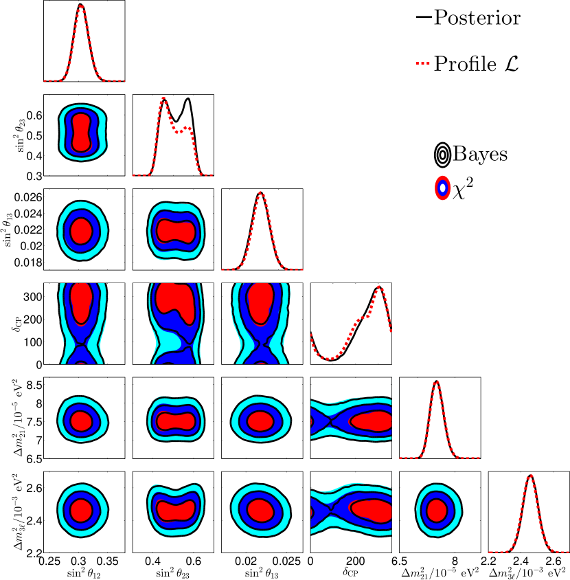
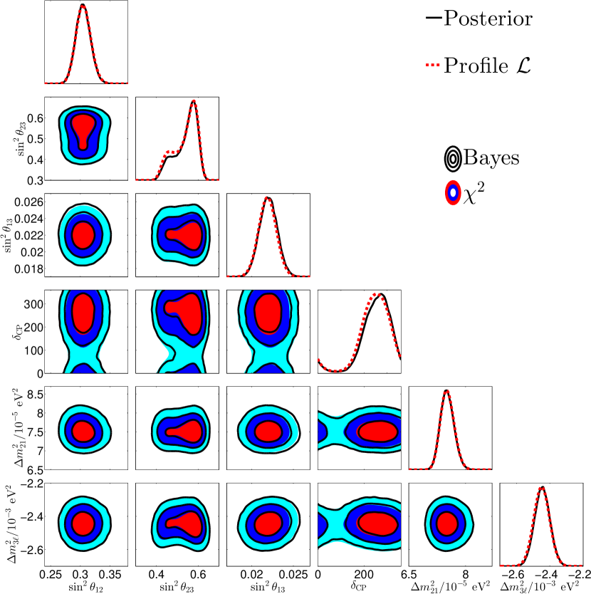
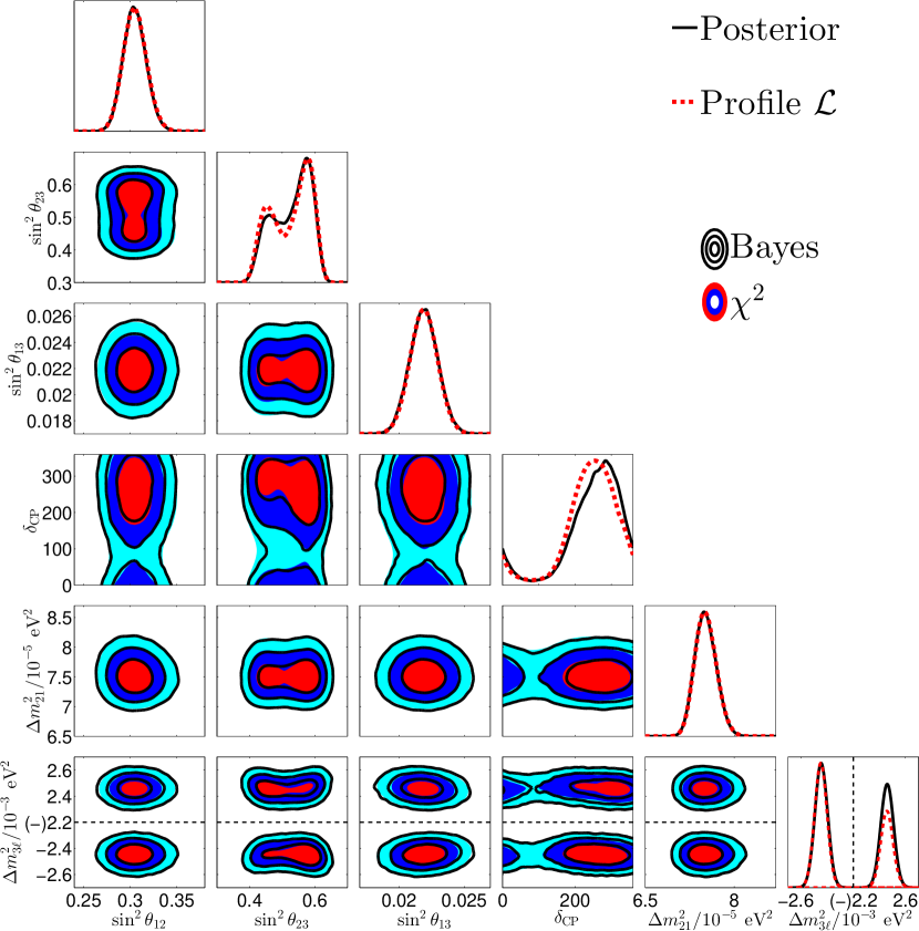
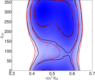
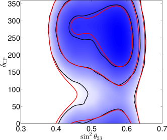
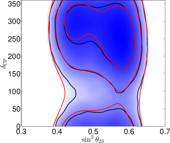
The results are shown in Fig. 1 for NO, Fig. 2 for IO, and Fig. 3 for MO. The posterior distribution for MO is simply the average of the NO and IO posteriors, weighted by the posterior probabilities of the orderings,

$$\Pr(\mathbf{\Theta}|\mathbf{D},{\rm MO})=\sum_{O={\rm NO,IO}}\Pr(\mathbf{\Theta}|\mathbf{D},O)\Pr(O|\mathbf{D}).$$ (10)

From these figures, we conclude that the absolute values of the two mass-square differences, as well as the mixing angles, $s^{2}_{12}$, and $s^{2}_{13}$, are well-measured and the posteriors of these parameters are Gaussian to a very good approximation.

We list in Tab. 2 different point estimates for each of these parameters: the global maximum likelihood (which is the best fit point, bfp, of the $\chi^{2}$ analysis), the point at which the marginal likelihood is maximal, and the posterior mean and median. The table also contains measures of the uncertainty of each parameter in the form of the 1$\sigma$ and 3$\sigma$ Bayesian credible intervals as well as the corresponding $\chi^{2}$ allowed regions at the same CL (which we also call $\chi^{2}$ intervals for simplicity) which are identical to those given in Ref. Gonzalez-Garcia:2014bfa . As seen in the table, for these four parameters their Bayesian point estimates and uncertainties are practically indistinguishable from their $\chi^{2}$ counterparts. Thus we conclude that the present determination of these four parameters is very robust under variations of the statistical analysis and prior assumptions.

Normal Ordering
	Point Estimates				$\chi^{2}$ Intervals		Bayes Credible Intervals
	bfp	$\begin{matrix}{\rm max\;of}\\[-5.69046pt] {\cal L}_{\rm marg}\end{matrix}$	mean	median	1$\sigma$ CI	3$\sigma$ CI	1$\sigma$ CI	3$\sigma$ CI
$\sin^{2}\theta_{12}$	0.304	0.304	0.305	0.305	[0.292,0.317]	[0.270,0.344]	[0.292,0.317]	[0.269, 0.344]
$\sin^{2}\theta_{13}$	0.0218	0.0218	0.0218	0.0218	[0.0208,0.0228]	[0.0186,0.0250]	[0.0207,0.0228]	[0.0187,0.0250]
$\frac{\Delta m^{2}_{21}}{10^{-5}{\rm eV}^{2}}$	7.5	7.5	7.5	7.5	[7.33,7.69]	[7.02,8.07]	[7.33,7.69]	[7.03,8.09]
$\frac{\Delta m^{2}_{3\ell}}{10^{-3}{\rm eV}^{2}}$	2.457	2.460	2.459	2.459	[2.417,2.504]	[2.317,2.607]	[2.414,2.506]	[2.320,2.601]
Inverted Ordering
$\sin^{2}\theta_{12}$	0.304	0.305	0.305	0.305	[0.292,0.317]	[0.270,0.344]	[0.292,0.317]	[0.269,0.344]
$\sin^{2}\theta_{13}$	0.0219	0.0219	0.0220	0.0220	[0.0209,0.0230]	[0.0188,0.0251]	[0.0209,0.0231]	[0.0189,0.0252]
$\frac{\Delta m^{2}_{21}}{10^{-5}{\rm eV}^{2}}$	7.5	7.5	7.5	7.5	[7.33,7.69]	[7.02,8.07]	[7.33,7.68]	[7.02,8.09]
$\frac{\Delta m^{2}_{3\ell}}{10^{-3}{\rm eV}^{2}}$	- 2.449	- 2.445	- 2.445	- 2.445	[-2.496,-2.401]	[-2.590,-2.307]	[-2.492,-2.400]	[-2.584,-2.308]

Table 2: Comparison of the results of $\chi^{2}$ and Bayesian analysis in the framework of three-flavor oscillations. For comparison of the determination of $\theta_{23}$ and $\delta_{\rm CP}$ see Sec. 4 and  5.

Considering the comparison between mass orderings, we find that, assuming the same prior probability for both, their posterior probabilities are also very similar, the posterior probability of IO in this case given by

$$\frac{\Pr(\mathbf{D}|\rm IO)}{\Pr(\mathbf{D}|\rm IO)+\Pr(\mathbf{D}|\rm NO)}=\frac{\mathcal{Z}_{\rm IO}}{\mathcal{Z}_{\rm IO}+\mathcal{Z}_{\rm NO}}=0.55.$$ (11)

The Bayes factor (which is independent of the prior on the ordering) is:

$$\log\mathcal{B}=\log\frac{\mathcal{Z}_{\rm NO}}{\mathcal{Z}_{\rm IO}}=\log\left(\frac{0.45}{0.55}\right)=-0.2,$$ (12)

i.e., there is a non-meaningful preference for inverted ordering. For comparison, the $\chi^{2}$ analysis finds $\Delta\chi^{2}=\chi^{2}_{\rm min}(\rm{NO})-\chi^{2}_{\rm min}(\rm{IO})\simeq 0.97$. Trivially, this gives $\Delta{\rm AIC}/2=0.5$ in favor of IO, which is also what $\log\mathcal{B}$ would be if the likelihoods would have identical shapes. In summary, both $\Delta\chi^{2}$ and the Bayesian model comparison agree that there is no evidence for any of the mass ordering in the present data. However one must not forget that since the mass ordering is not a continuous parameter, $\Delta\chi^{2}$ should not have a $\chi^{2}$ distribution, and hence the quantification of the degree of favouring/disfavouring of a given ordering based on the corresponding $\Delta\chi^{2}$ is not fully justified (see Ref. Blennow:2013oma for further discussion).

Finally we notice that figures 1–3 show some differences between the results of the $\chi^{2}$ and Bayesian analyses where $\delta_{\rm CP}$ or $s^{2}_{23}$ are involved. For example, we see that the marginalization over $\delta_{\rm CP}$ pulls the bulk of the posterior of $s^{2}_{23}$ more into the second octant. Motivated by these differences we present a more detailed study of the results on $s^{2}_{23}$, $\delta_{\rm CP}$, and CP-violation in the following sections.

Figure 1: One-dimensional posterior distributions (black full lines) and two-dimensional $1\sigma$, $2\sigma$ and $3\sigma$ Bayesian credible regions (black void contours). The figure also shows the one-dimensional profile likelihoods (red dashed curves) and two-dimensional $\chi^{2}$ regions (coloured filled regions) from Ref. Gonzalez-Garcia:2014bfa .

Figure 2: Same as Fig. 1 but for IO.

Figure 3: Same as Fig. 1 but for MO.

4 Determination of $s^{2}_{23}$

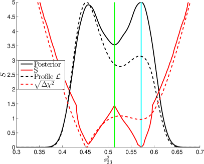
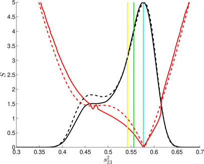
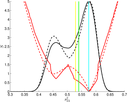
In this section we study the determination of $s^{2}_{23}$ in more detail. To do so, in Fig. 4 we plot the Bayesian marginal posterior distribution (which in this case is proportional to the marginal likelihood) of $s^{2}_{23}$ for all orderings together with the $S$ of the credible intervals (see Eqs. (7) and (8)), as well as the profile likelihood and $\sqrt{\Delta\chi^{2}}$ (the nominal significance under the assumption of a standard $\chi^{2}$ distribution).

We note that the Bayesian analysis generally prefers the second octant and it does so more than the $\chi^{2}$ analysis, in particular for NO. Although the credible and confidence levels differ in the vicinity of the two peaks, both peaks are within the $2\sigma$ region, and outside of that region the difference between the two analyses is rather small. Typically, the low-credibility Bayesian regions are larger than the small-$\chi^{2}$ regions, while the high-credibility Bayesian regions are smaller than the large-$\chi^{2}$ ones. This is just what is expected if the likelihood contains a relatively sharp peak on top of a broader plateau containing significant posterior probability.

For completeness, in addition to being displayed in Fig. 4, we also give the point estimates of $s^{2}_{23}$ in Tab. 3, namely, the global maximum likelihood, the maximum of the marginal likelihood, and the posterior mean and median. In Tab. 4 the measures of uncertainty are given in the form of the posterior standard deviation, as well as credible intervals corresponding to Fig. 4, and the regular $\chi^{2}$ intervals.

Figure 4: Bayesian posterior/marginal likelihood (black solid), plotted together with the profile likelihood (black dashed), from Ref. Gonzalez-Garcia:2014bfa (both normalized to their maximal value). The number number of $\sigma^{\prime}s$)(red solid), and $\sqrt{\Delta\chi^{2}}$ (red dashed). Posterior mean (yellow line), median (green), and maximum of the marginal likelihood (cyan). NO (top left), IO (top right), MO (bottom).

Ordering	Global max	max of $\mathcal{L}_{\rm marg}$	mean	median
NO	$0.452$	$0.571$	$0.515$	$0.516$
IO	$0.579$	$0.576$	$0.541$	$0.555$
MO	$0.579$	$0.576$	$0.529$	$0.542$

Table 3: Point estimates of $s^{2}_{23}$.

Ordering	Method	st. dev.	$1\sigma$ CI	$2\sigma$ CI	$3\sigma$ CI
NO	Bayes	$0.0585$	$[0.433,0.496],[0.530,0.594]$	$[0.415,0.613]$	$[0.389,0.637]$
	$\chi^{2}$	-	$[0.424,0.505],[0.554,0.582]$	$[0.402,0.622]$	$[0.381,0.643]$
IO	Bayes	$0.0534$	$[0.514,0.612]$	$[0.429,0.622]$	$[0.400,0.640]$
	$\chi^{2}$	-	$[0.541,0.604]$	$[0.416,0.625]$	$[0.388,0.644]$
MO	Bayes	$0.0574$	$[0.449,0.476],[0.516,0.607]$	$[0.422,0.618]$	$[0.393,0.638]$
	$\chi^{2}$	-	$[0.448,0.458],[0.541,0.604]$	$[0.407,0.625]$	$[0.385,0.644]$

Table 4: Standard deviations, credible intervals, and $\chi^{2}$ intervals for $s^{2}_{23}$.

4.1 Octants of $\theta_{23}$ and maximal mixing

A related question is that of which octant $\theta_{23}$ belongs to, i.e., whether $s_{23}^{2}$ is larger or smaller than $0.5$. With some similarity to the comparison of mass orderings, this is also a comparison of two non-nested models with the same number of parameters (although they are “adjacent”), and so one cannot expect difference between the $\chi^{2}$ minima between the two octants to have a $\chi^{2}$ distribution. In a Bayesian analysis, the comparison is however straightforward, by simply integrating the likelihoods over each of the octants.

In addition, one can also consider maximal mixing, $s_{23}^{2}=0.5$, as a realistic model, either exactly or approximately. From a statistical viewpoint, a model with a fixed value of a parameter can also be interpreted as a model where there is some non-zero, but negligible (compared to any experimental sensitivity) deviation from the fixed value hoeting1999 . Using any of these viewpoints, i.e., by either considering exact maximal mixing as a possible scenario, or alternatively as simply a very good approximation, one can make a comparison with the octants.

As always, a model with additional parameters will be punished for this extra complexity. In the present case, this punishment is uniquely fixed by the compactness of the space of the allowed values of $s^{2}_{23}$. The Bayes factors between the second and first octants, as well as between non-maximal and maximal mixing, are given in Tab. 5.

		NO	IO	MO
2nd octant vs. 1st	$\log\mathcal{B}$	$0.3$	$1.2$	$0.7$
	$\Delta{\rm AIC}/2$	$-0.5$	$1$	$0.5$
	$\Delta\chi^{2}$	$-0.9$	$2.0$	$1.0$
Non-maximal vs. maximal	$\log\mathcal{B}$	$-1.5$	$-1.2$	$-1.3$
	$\Delta{\rm AIC}/2$	$-0.5$	$0.0$	$0.0$
	$\Delta\chi^{2}$	$0.9$	$2.0$	$2.0$

Table 5: Model comparison for different assumptions on $s^{2}_{23}$. Logarithms of Bayes factors, the comparable differences in the AIC, and differences in $\chi^{2}$ minima. The sign is chosen such that positive values correspond to preference for first mentioned assumptions in each case, i.e., the 2nd octant and non-maximal mixing, respectively.

The second octant is weakly preferred over the first for the inverted ordering, but not in the normal and the mixed orderings. Using the AIC, with the values also given in Tab. 5, yields the same conclusions, although we remind the reader that interpreting the AIC as a model likelihood should be done with great care. Due to the relatively bad predictivity of the assumption of non-maximal mixing, maximal mixing is weakly preferred over non-maximal in all orderings. Note that $\Delta{\rm AIC}/2$ can never be smaller than $-1$ in this case, and these numbers close to that limit are simply saying that for no ordering is there any preference for non-maximal mixing.

If in the future the uncertainty on $s^{2}_{23}$ keeps on being reduced while maximal mixing continues to be allowed, at some point reducing the uncertainty further is pointless for the purpose of determining whether maximal-mixing is the correct model. Bayesian model comparison gives a quantification of at which point this is the case, which is when the evidence in favour of non-maximal mixing becomes strong.

5 Exploring $\delta_{\rm CP}$ and CP-violation

Figure 5: Left plots: same as Fig. 4 for $\delta_{\rm CP}$. Right plots: Same as left plots, but with only posterior and profile likelihood and plotted in polar coordinates. For clarity, half of the maximal radius corresponds to zero function value.

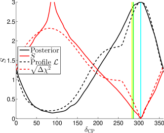
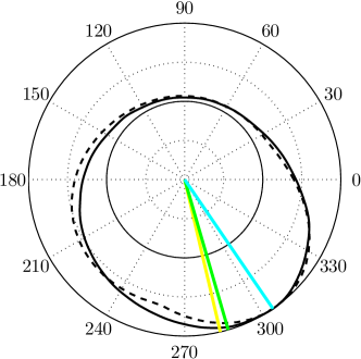
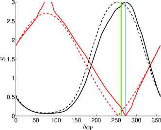
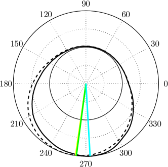
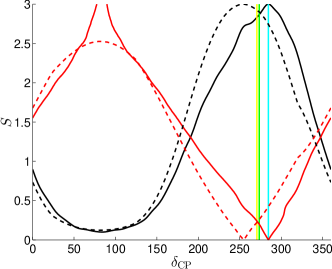
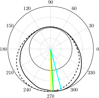
In this section we study the determination of $\delta_{\rm CP}$ in more detail. In the left panels of Fig. 5 we plot the Bayesian marginal posterior distribution of $\delta_{\rm CP}$ for all orderings together with the $S$ of the credible intervals, as well as the profile likelihood and $\sqrt{\Delta\chi^{2}}$. For NO, the marginal and profile likelihoods have their maximum at about the same value of $\delta_{\rm CP}$, but for IO and MO, the Bayesian analysis prefers larger $\delta_{\rm CP}$. Comparing $S$ with $\sqrt{\Delta\chi^{2}}$, the difference is not that large, apart from the shift just mentioned, and the fact that $S$ diverges near $\delta_{\rm CP}\simeq 90^{\circ}$, while $\sqrt{\Delta\chi^{2}}$ is bounded by about $2.5$.

In the right panels of Fig. 5 the marginal and profile likelihoods are plotted again, but in a polar coordinate system which better reflects its circular nature. We note that in a frequentist analysis the fact that $\delta_{\rm CP}$ is a phase and a circular, periodic variable will affect distributions of test statistics Blennow:2014sja ; Elevant:2015ska . For the present data $\sqrt{\Delta\chi^{2}}$ is expected to be a poor approximation of the frequentist significance, and typically the true significance will be higher than the naive expectation. Hence, Fig. 5 does not give a direct comparison of frequentist and Bayesian results.

In the Bayesian analysis, however, the circular nature of $\delta_{\rm CP}$ does not affect the posterior distributions or its interpretation. Nevertheless, it still needs to be taken into account if one wants to make summaries of the posterior in terms of point estimates such as the mean, median, or measures of dispersion such as the standard deviation. This is because the normal, linear definitions of these quantities will depend on the arbitrary choice of origin for $\delta_{\rm CP}$ Jammalamadaka:2001 ; Mardia:2009 ; Fisher:1995 .

In this respect a useful summary of the distribution of $\delta_{\rm CP}$ is given by the first moment,

$$m_{1}=\langle e^{i\delta_{\rm CP}}\rangle,$$ (13)

with $\langle\cdot\rangle$ denoting the mean (indeed, it is $e^{i\delta_{\rm CP}}$ which enters the mixing matrix). The appropriate analogues of the mean and median of $\delta_{\rm CP}$ are the circular mean and circular median. The first one is given by the argument of the first moment,

$$\overline{\delta_{\rm CP}}=\arg m_{1}=\arg\langle e^{i\delta_{\rm CP}}\rangle,$$ (14)

while the second is defined as the endpoint closer to mean of the diameter of the circle that has $0.5$ probability on each of its sides. These point estimates are summarized in Tab. 6 together with the likelihood maxima, and their values are plotted in Fig. 5.

In what respects characterization of the dispersion, besides the credible intervals, if one wants to have a characterization similar to that provided by the linear standard deviation, one can make use of the fact that $R=|m_{1}|$ gives a reasonable measure of dispersion, with $R=0$ for a uniform distribution and $R=1$ for a degenerate one. However, it could be preferable and more easily interpretable to have such a measure which is an expected deviation in radians. Noting that the standard linear variance is the expectation of the Euclidean distance squared from the mean, in general one could use

$$V=\langle d^{2}(\delta_{\rm CP},\overline{\delta_{\rm CP}})\rangle$$ (15)

to obtain a dispersion, where $d$ is some metric on the circle. The usual linear metric $d(\alpha,\beta)=|\alpha-\beta|$ is not invariant with respect to choice of origin, but one can take instead $d$ as the minimum arc length between $\alpha$ and $\beta$, also called the great-circle distance. Hence, one can simply take $\sigma=\sqrt{\langle d^{2}(\delta_{\rm CP},\overline{\delta_{\rm CP}})\rangle}$ as the variance.

Another metric one can use is the one inherited from the Euclidean embedding,

$$d^{\prime}(\alpha,\beta)^{2}=|e^{{\rm i}\alpha}-e^{{\rm i}\beta}|^{2}=(\sin\alpha-\sin\beta)^{2}+(\cos\alpha-\cos\beta)^{2}=2(1-\cos(\alpha-\beta)).$$ (16)

Then, the variance becomes

$$V=\langle d^{\prime}(\delta_{\rm CP},\overline{\delta_{\rm CP}})^{2}\rangle=\langle 2(1-\cos(\delta_{\rm CP}-\overline{\delta_{\rm CP}}))\rangle=2(1-R),$$ (17)

since $R=\langle\cos(\delta_{\rm CP}-\overline{\delta_{\rm CP}})\rangle$. To get the equivalent deviation as an angle away from the mean, we solve $V=2(1-\cos\sigma^{\prime})$, giving simply

$$\sigma^{\prime}=\arccos R,$$ (18)

which is then the deviation from the mean which has the same distance squared as the expectation over the distribution. These measures of dispersion, together with the corresponding credible intervals, are show in Tab. 7.

Ordering	Global max $[{}^{\circ}]$	Max of $\mathcal{L}_{\rm marg}$ $[{}^{\circ}]$	mean $[{}^{\circ}]$	median $[{}^{\circ}]$
NO	306	$304$	$289$	$286$
IO	254	$273$	$262$	$262$
MO	254	$289$	$271$	$272$

Table 6: Point estimates of $\delta_{\rm CP}$. The mean and median are the corresponding circular quantities.

Ordering	Method	$\sigma/\sigma^{\prime}[{}^{\circ}]$	$1\sigma$ CI $[{}^{\circ}]$	$2\sigma$ CI $[{}^{\circ}]$	$3\sigma$ CI $[{}^{\circ}]$
NO	Bayes	$65/58$	$[223,350]$	$[42,139]^{c}$	$[84,94]^{c}$
	$\chi^{2}$	-	$[234,346]$	$[33,131]^{c}$	-
IO	Bayes	$56/51$	$[207,319]$	$[9,146]^{c}$	$[70,90]^{c}$
	$\chi^{2}$	-	$[192,317]$	$[8,142]^{c}$	-
MO	Bayes	$61/55$	$[211,333]$	$[28,144]^{c}$	$[76,90]^{c}$
	$\chi^{2}$	-	$[192,317]$	$[16,142]^{c}$	-

Table 7: Measures of dispersion and credible intervals. Here, $I^{c}$ is the complement of $I$, i.e., all values of $\delta_{\rm CP}$ not contained in $I$.

Figure 6: Jarlskog invariant and its maximal value for all orderings. NO (top), IO (middle), MO (bottom).

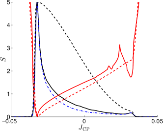
The presence of CP violation can also be studied in terms of the Jarlskog invariant, $J_{\rm CP}$, which, in the standard parameterization, is given by

$$J_{\rm CP}=J^{\rm max}_{\rm CP}\sin\delta_{\rm CP}=c_{12}s_{12}c_{23}s_{23}c_{13}^{2}s_{13}\sin\delta_{\rm CP}.$$ (19)

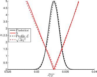
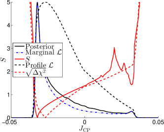
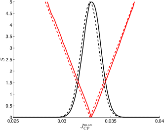
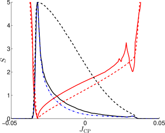
We plot in Fig. 6 the Bayesian marginal posterior distribution of $J_{\rm CP}$ and $J^{\rm max}_{\rm CP}$ for all orderings together with the $S$ of the credible intervals, as well as the profile likelihood and $\sqrt{\Delta\chi^{2}}$. We note that these are derived parameters, and so their priors and posteriors are determined by those of the free oscillation parameters. In particular, their priors are not exactly uniform. For $J^{\rm max}_{\rm CP}$ (the left panels) the prior is very close to uniform, and from the figure we see that it is so well constrained that it is perfectly Gaussian and agrees with the profile likelihood.

For $J_{\rm CP}$ (right panels of Fig. 6), we plot both the posterior and the marginal likelihood, and we observe a difference, although it is not very large. A much larger difference is observed between these and the profile likelihood, which translates into a difference in the corresponding CL’s ($S$ and $\sqrt{\Delta\chi^{2}}$). However, this difference is much smaller than one could naively expect form the differences in posterior versus the profile likelihood, the reason for this being that the Bayesian results are a function of the total probability contained in a region, and the sharp peak in the posterior still contains relatively little probability.

That the posterior of $J_{\rm CP}$ shows peaks towards the edges of the distribution is simply because the density of $|\sin\delta_{\rm CP}|$ is larger for those values. This is not canceled out in the marginal likelihood because $J^{\rm max}_{\rm CP}$ has a broad prior, which means that so has $J_{\rm CP}$. Of course, the symmetry around $J_{\rm CP}=0$ is broken by the information on $\delta_{\rm CP}$ supplied by the data, which then means that negative values of $J_{\rm CP}$ are preferred, and more strongly so than in the $\chi^{2}$ analysis. Note that since we do not have any freedom left in choosing our priors on the oscillation angles and phase, this is in some sense a robust consequence of using consistent Bayesian inference.

5.1 CP-violation vs CP-conservation

In the same way as maximal mixing, one can consider either exact CP-conservation as a possible scenario, or alternatively simply CP-conservation as a very good approximation, and compare the models:

• $M_{\rm CPC}^{1}$: $\delta=0$

• $M_{\rm CPC}^{2}$: $\delta=180^{\circ}$

• $M_{\rm CPC}:M_{\rm CPC}^{1}$ or $M_{\rm CPC}^{2}$ (with equal priors)

• $M_{\rm CPV}$: $\delta\in[0^{\circ},360^{\circ}]\setminus\{0^{\circ},180^{\circ}\}$, with prior $\pi(\delta_{\rm CP})=1/360^{\circ}$.

Note that these assumptions on CPC and CPV are unambiguously defined in the sense that they do not depend on a parameterization, and that the prior on $\delta_{\rm CP}$ in $M_{\rm CPV}$ is uniquely given by the Haar measure. Hence, there is essentially no flexibility remaining in the choice of prior. Due to this fact and the compact nature of the parameter space, the normal pitfalls of model comparison, i.e., the potentially large and prior dependent penalty acquired for additional parametric complexity, are avoided, or at least heavily mitigated.

This unusually robust (fixed in size) and small penalty for the additional parameter means that the Bayesian analysis is expected to be more powerful at detecting CPV than it normally is at detecting a new physical effect. Hence, when comparing with a $\chi^{2}$ analysis, a smaller significance or value of $\Delta\chi^{2}$ than normally should be needed for robust, Bayesian, detection of CPV. Equivalently, a certain value of $\Delta\chi^{2}$ would lead to a stronger Bayesian evidence of CPV than what the same $\Delta\chi^{2}$ would yield in a different setting.

Interestingly, also the true frequentist significance of CP-violation is expected to be stronger than the naive expectation Elevant:2015ska , although the details depend significantly on the (unknown) value of $s^{2}_{23}$ assumed to be true . This does not happen in a Bayesian analysis, which also does not depend on any distributions of test statistics under repeated experiments, but only on likelihood of the data which was actually observed.

The likelihoods of the different assumptions on $\delta_{\rm CP}$, in the usual form of logarithms of Bayes factors, $\log(\mathcal{Z}/\mathcal{Z}_{\rm CPV})$ relative to $M_{\rm CPV}$ are shown in Tab. 8, together with the AIC and difference in $\chi^{2}$. Although technically CP-violation is preferred in all cases, in none of the cases is the evidence even weak. Notice also that since $\delta_{\rm CP}$ is relatively unconstrained, the preference for CPV is even smaller using the AIC than in the Bayesian analysis.

		NO	IO	MO
$M_{\rm CPC}^{1}$	$\log\mathcal{B}$	$-0.1$	$-0.8$	$-0.4$
	$\Delta{\rm AIC}/2$	$0.1$	$-0.7$	$-0.4$
	$\Delta\chi^{2}$	$-1.8$	$-3.4$	$-2.8$
$M^{2}_{\rm CPC}$	$\log\mathcal{B}$	$-0.4$	$-0.1$	$-0.2$
	$\Delta{\rm AIC}/2$	$0.1$	$0.3$	$0.3$
	$\Delta\chi^{2}$	$-1.8$	$-1.5$	$-1.5$
$M_{\rm CPC}$	$\log\mathcal{B}$	$-0.2$	$-0.4$	$-0.3$
	$\Delta{\rm AIC}/2$	$0.1$	$0.3$	$0.3$
	$\Delta\chi^{2}$	$-1.8$	$-1.5$	$-1.5$

Table 8: Model comparison for different assumptions on $\delta_{\rm CP}$. Logarithms of Bayes factors relative to $M_{\rm CPV}$, the comparable differences in the AIC, and differences in $\chi^{2}$ as $\Delta\chi^{2}=\chi^{2}_{\rm M_{CPV}}-\chi^{2}_{\rm M^{i}_{CPC}}$. For all variables, positive values would indicate preference of the corresponding $M^{i}_{\rm CPC}$ over $M_{\rm CPV}$.

6 Correlation between $s_{23}^{2}$ and $\delta_{\rm CP}$

In this section we discuss the possible quantification of the correlation between $\sin^{2}\theta_{23}$ and $\delta_{\rm CP}$. The posterior in the $s^{2}_{23}-\delta_{\rm CP}$ plane for all the orderings is plotted in Fig. 7, together with the credible regions and $\chi^{2}$ contours. Although the difference between the Bayesian and $\chi^{2}$ analysis does not appear to be extremely large, there are some things which a Bayesian analysis makes possible which cannot be done in a $\chi^{2}$ analysis. In particular, as seen in the figure, it is clear that $s^{2}_{23}$ and $\delta_{\rm CP}$ are not independent, and it will be interesting to quantify if the degeneracy between them is something which persists in future experiments. In a $\chi^{2}$ analysis, quantifying the “correlation” between two parameters is typically limited to fitting a two dimensional Gaussian at the best-fit point. In a Bayesian analysis, global measures of association such as the standard Pearson product-moment correlation coefficient are available. However, this one only measures linear association, and is hence less useful when there are non-linear trends involved, including multi-modality. In particular it is possible for two highly dependent variables to have very small value of the Pearson correlation. Furthermore, in the present case, it fails in an even worse manner since the Pearson correlation is not circular invariant, i.e., its value depends on the arbitrary choice of origin for $\delta_{\rm CP}$. In what respects $\theta_{23}$ one can treat $\theta_{23}$ as circular variable or use instead the linear variable $s^{2}_{23}$.

Figure 7: Posterior in the $s^{2}_{23}-\delta_{\rm CP}$ plane (blue shading), $1\sigma$, $2\sigma$, $3\sigma$ credible regions (black) $\chi^{2}$ contours (red dashed). NO (top left), IO (top right), MO (bottom).

So let us focus on how to define a correlation coefficient which can overcome these limitations. Typically a correlation coefficient will aim to quantify how much of the variation in one variable can be explained by the variation in another one. For example, to what extent the linear relation $\langle Y|X=x\rangle=ax+b$ is responsible for the variation in $Y$ (which leads to the standard Pearson correlation coefficient). Similarly one can consider circular-circular associations between two circular variables $\Theta$ and $\Phi$ (in this case $\delta_{\rm CP}$ and $\theta_{23}$), circular-linear association, predicting the expectation of $\Theta$, given $X=x$ , or linear-circular association, predicting the expectation of $X$, given $\Theta=\theta$ (in these cases $X=\sin^{2}\theta_{23}$).

Many measures of correlation involving circular variables already exist in the literature (see Jammalamadaka:2001 ; Mardia:2009 ; Fisher:1995 ; Jones2006176 ). For two circular variables a simple one is

$$\rho_{\rm cc}=\frac{\langle\sin(\Theta-\bar{\Theta})\sin(\Phi-\bar{\Phi})\rangle}{\sqrt{\langle\sin^{2}(\Theta-\bar{\Theta})\rangle\langle\sin^{2}(\Phi-\bar{\Phi})\rangle}},$$ (20)

where the bar denotes the circular mean. This has many properties in common with the linear version, such as being confined to the interval $[-1,1]$, it is zero if the variables are independent, and it numerically agrees with the linear version for concentrated distributions.

An alternative, but slightly more complex, correlation coefficient for two circular variables is the T-linear one of Ref. Fisher:1983 ,

$$\rho_{\rm T}=\frac{\langle\sin(\Theta_{1}-\Theta_{2})\sin(\Phi_{1}-\Phi_{2})\rangle}{\sqrt{\langle\sin^{2}(\Theta_{1}-\Theta_{2})\rangle\langle\sin^{2}(\Phi_{1}-\Phi_{2})\rangle}},$$ (21)

where $\Theta_{1}$ and $\Theta_{2}$ are treated as two independent copies of $\Theta$, and similarly for $\Phi$.

Also for linear-circular association, one can split the circular variable into its sine and cosine and consider the multiple correlation coefficient between $X$ and $(\sin\Theta,\cos\Theta)$, giving

$$\rho^{2}_{\rm lc}=\frac{\rho^{2}_{xc}+\rho^{2}_{xs}-2\rho_{xs}\rho_{xc}\rho_{cs}}{1-\rho^{2}_{cs}},$$ (22)

with $\rho_{xc}=\rho(x,\cos y)$, $\rho_{xs}=\rho(x,\sin y)$, $\rho_{cs}=\rho(\cos y,\sin y)$ being standard linear coefficients. We notice that being defined by a square, only $|\rho_{\rm lc}|$ is known and hence gives no information on the “sign” or “direction” of the association.

While the above measures of association overcome the problem of the circular invariance they are still only sensitive to a limited kind of association, and it is possible for them to be zero even when the variables are highly dependent on each other. It could hence be of interest to have a measure which can quantify any type of dependence, and which will only be zero when the variables are independent. Such a measure, based on information theory, is the mutual information Murphy:2012 ; PhysRevE.69.066138 ; Moddemeijer1989233 ; Steuer01102002 . This is information gained by knowing the full distribution $P(x,y)$ rather than only the marginal distributions $P(x)$, and $P(y)$, or equivalently, the average information gained on $X$ by knowing the value of $Y$ (and vice versa). This can be expressed as the so-called Kullback-Liebler divergence between $P_{X,Y}$ and the product $P_{X}P_{Y}$,

$$I(X,Y)=\int P(x,y)\log\frac{P(x,y)}{P(x)P(y)}{\rm d}x{\rm d}y.$$ (23)

Using the natural logarithm gives the result in nats, while one obtains the results in bits by using base 2. It holds that $I(X,Y)\geq 0$ with equality if and only if $X$ and $Y$ are independent. Next, in order to make the connection with the standard correlation coefficient, we note that for a two-dimensional Gaussian distribution (for which no correlation is equivalent to independence), $I=\log(1/\sqrt{1-\rho^{2}})$, and so we define

$$\rho^{2}_{I}=1-e^{-2I}.$$ (24)

We now have constructed a correlation coefficient which is independent of any boundary conditions on the variables and is invariant under arbitrary univariate redefinitions of $x$ and $y$ (which the others are not). As the previous coefficients it also reduces to the standard Pearson coefficient in the limit of a concentrated Gaussian distribution. However, like $|\rho_{\rm cl}|$, it only measures the degree of dependence, but not any “direction” of the association.

Our estimates of the different correlation coefficients are given in Tab. 9. For all measures, we find stronger correlation in NO than in IO, typically significantly so (with the exception of $\rho_{\rm T}$). Furthermore, the two signed circular-circular measures have significantly smaller absolute values than the others, and for these we also find that in MO the correlation is actually larger than both NO and IO, which is not the case for the others. We note that all are smaller than or equal in size of $|\rho_{I}|$. This is somehow expected as $|\rho_{I}|$, in some sense, measures “all” the dependence between $\delta_{\rm CP}$ and $s^{2}_{23}$.

	NO	IO	MO
$\rho_{\rm cc}$	$-0.20$	$-0.15$	$-0.21$
$\rho_{\rm T}$	$-0.14$	$-0.13$	$-0.16$
$|\rho_{\rm cl}|$	$0.27$	$0.16$	$0.23$
$|\rho_{I}|$	$0.30$	$0.18$	$0.26$

Table 9: Different correlation coefficients between $s^{2}_{23}$ and $\delta_{\rm CP}$.

7 Summary

We have presented the results of a Bayesian global analysis of solar, atmospheric, reactor and accelerator neutrino data in the framework of three-neutrino oscillations and compared them with those from the standard $\chi^{2}$ analysis in NuFIT 2.0 nufit . The results are summarized Fig. 1 for NO, Fig. 2 for IO, and Fig. 3 for MO where we compare the relevant Bayesian quantities (the posterior distribution and two-dimensional Bayesian credible regions) with the profile-likelihood and the two dimensional $\chi^{2}$ allowed regions.

We found that the four parameters $\Delta m^{2}_{3\ell}$, $\Delta m^{2}_{21}$, $s^{2}_{12}$, and $s^{2}_{13}$, are well-measured and their posterior distributions are Gaussian to a very good approximation. The corresponding Bayesian credibility intervals at a given CL are also very similar to the $\chi^{2}$ allowed regions at the same CL, as seen in Table 2.

We found some differences between the results of the $\chi^{2}$ and Bayesian analysis where $\delta_{\rm CP}$ or $s^{2}_{23}$ are involved. In particular, the marginalization over $\delta_{\rm CP}$ pulls the bulk of the posterior of $s^{2}_{23}$ more into the second octant which has some effect on the ranges of parameter estimates and the quality of the description between octants. We study the determination of $\theta_{23}$ in more detail in Sec. 4 and we conclude that the Bayesian analysis generally prefer the second octant more so than the $\chi^{2}$ analysis, in particular for NO. The credible and confidence levels differ in the vicinity of the two peaks but both peaks are within the $2\sigma$ regions. Altogether the low-credibility Bayesian regions are larger than the small-$\chi^{2}$ regions, while the high-credibility Bayesian regions are smaller than the large-$\chi^{2}$ ones.

In what respects the present determination of $\delta_{\rm CP}$, presented in Sec. 5, we found that for NO, the marginal and profile likelihoods have their maximum at about the same value of $\delta_{\rm CP}$, but for IO and MO, the Bayesian analysis prefers slightly larger values of $\delta_{\rm CP}$. Also, unlike the $\chi^{2}$ interval, the 3$\sigma$ Bayesian credible interval do not contain the full range of $\delta_{\rm CP}$ but some values near $\pi/2$ are not included. We have also introduced and quantified two measures of the dispersion of $\delta_{\rm CP}$ equivalent to the linear standard deviations but valid for a circular variable.

In addition, we have studied the Jarlskog invariant, $J_{\rm CP}$, as well as its maximal value over $\delta_{\rm CP}$ and find that the posterior distribution of $J^{\rm max}_{\rm CP}$ is perfectly Gaussian and agrees with the profile likelihood. For $J_{\rm CP}$ large differences appear between the posterior distribution and the profile likelihood and lead to some difference in the corresponding CL intervals. In particular we find that negative values of $J_{\rm CP}$ are preferred in both analysis but more strongly in the Bayesian than in the $\chi^{2}$ analysis.

The possible quantification of the correlation between $\theta_{23}$ and $\delta_{\rm CP}$ taking into account their circular nature has been discussed in Sec. 6. In particular, we have introduced a new correlation coefficient, $\rho_{I}$, defined in terms of the mutual information, which is independent of any boundary conditions on the variables and is invariant under arbitrary univariate redefinitions of them. Quantitatively we always find stronger correlation between $\delta_{\rm CP}$ and $\theta_{23}$ in NO than in IO.

Finally, we note that a Bayesian analysis is particularly suited for comparing how much better one model describes the data compared to another model, a comparison which is quantified in terms of the Bayes factor of the two models (assuming both models to be equally probable a priori). We have applied this to the comparison between the mass orderings, the octant of $\theta_{23}$, and to the presence of CP violation with the following conclusions:

• In what regards the comparison between both orderings, we find that, assuming the same prior probability for both, their posterior probabilities are also very similar: 0.55 for IO and 0.45 for NO with a logarithm of Bayes factor of $-0.2$, which implies that slight preference for inverted ordering is not statistically meaningful.

• Applied to the preference for the octant of $\theta_{23}$ we find that the second octant is weakly preferred over the first for the inverted ordering, but not in the normal nor in the case of no assumption or knowledge on the ordering. Also due to the relatively bad predictivity of the assumption of non-maximal mixing, maximal mixing is weakly preferred over non-maximal in all orderings.

• As for CP violation we find that although technically CP-violation is preferred over CP conservation (either for $\delta_{\rm CP}=0$ or $\delta_{\rm CP}=\pi$), the corresponding value of the logarithm of the Bayes factor is always smaller than 1 in absolute value, i.e., the corresponding evidence is not even weak.

References

- (1) B. Pontecorvo, Neutrino experiments and the question of leptonic-charge conservation, Sov. Phys. JETP 26 (1968) 984–988
- (2) V. N. Gribov and B. Pontecorvo, Neutrino astronomy and lepton charge, Phys. Lett. B28 (1969) 493
- (3) M. C. Gonzalez-Garcia and M. Maltoni, Phenomenology with Massive Neutrinos, Phys. Rept. 460 (2008) 1–129, [arXiv:0704.1800]
- (4) Z. Maki, M. Nakagawa, and S. Sakata, Remarks on the unified model of elementary particles, Prog. Theor. Phys. 28 (1962) 870–880
- (5) M. Kobayashi and T. Maskawa, CP violation in the renormalizable theory of weak interaction, Prog. Theor. Phys. 49 (1973) 652–657
- (6) Particle Data Group Collaboration, J. Beringer et. al., Review of Particle Physics (RPP), Phys. Rev. D86 (2012) 010001
- (7) M. Gonzalez-Garcia, M. Maltoni, and T. Schwetz, Updated fit to three neutrino mixing: status of leptonic CP violation, JHEP 1411 (2014) 052, [arXiv:1409.5439]
- (8) F. Capozzi, G. Fogli, E. Lisi, A. Marrone, D. Montanino, et. al., Status of three-neutrino oscillation parameters, circa 2013, Phys.Rev. D89 (2014) 093018, [arXiv:1312.2878]
- (9) D. Forero, M. Tortola, and J. Valle, Neutrino oscillations refitted, Phys.Rev. D90 (2014), no. 9 093006, [arXiv:1405.7540]
- (10) NuFIT webpage, http://www.nu-fit.org
- (11) R. Trotta, Bayes in the sky: Bayesian inference and model selection in cosmology, Contemp. Phys. 49 (2008) 71--104, [arXiv:0803.4089]
- (12) M. Hobson et. al., eds., Bayesian methods in cosmology. Cambridge University Press, 2010
- (13) K. P. Burnham and D. R. Anderson, Model Selection and Multimodel Inference: A Practical Information-Theoretic Approach. Springer Science & Business Media, 2007
- (14) A. R. Liddle, Information criteria for astrophysical model selection, MNRAS 377 (May, 2007) L74--L78, [astro-ph/]
- (15) J. O. Berger, B. Liseo, and R. L. Wolpert, Integrated likelihood methods for eliminating nuisance parameters, Statistical Science 14 (02, 1999) 1--28
- (16) F. Feroz and M. Hobson, Multimodal nested sampling: an efficient and robust alternative to MCMC methods for astronomical data analysis, Mon. Not. Roy. Astron. Soc. 384 (2008) 449, [arXiv:0704.3704]
- (17) F. Feroz, M. Hobson, and M. Bridges, MultiNest: an efficient and robust Bayesian inference tool for cosmology and particle physics, Mon. Not. Roy. Astron. Soc. 398 (2009) 1601--1614, [arXiv:0809.3437]
- (18) F. Feroz, M. Hobson, E. Cameron, and A. Pettitt, Importance nested sampling and the MultiNest algorithm, arXiv:1306.2144
- (19) J. O. Berger, Statistical decision theory and Bayesian analysis. Springer-Verlag, 1985
- (20) N. Haba and H. Murayama, Anarchy and hierarchy, Phys. Rev. D63 (2001) 053010, [hep-ph/0009174]
- (21) B. T. Cleveland et. al., Measurement of the solar electron neutrino flux with the Homestake chlorine detector, Astrophys. J. 496 (1998) 505--526
- (22) F. Kaether, W. Hampel, G. Heusser, J. Kiko, and T. Kirsten, Reanalysis of the GALLEX solar neutrino flux and source experiments, Phys. Lett. B685 (2010) 47--54, [arXiv:1001.2731]
- (23) SAGE Collaboration, J. N. Abdurashitov et. al., Measurement of the solar neutrino capture rate with gallium metal. III: Results for the 2002–2007 data-taking period, Phys. Rev. C80 (2009) 015807, [arXiv:0901.2200]
- (24) Super-Kamiokande Collaboration, J. Hosaka et. al., Solar neutrino measurements in Super-Kamiokande-I, Phys. Rev. D73 (2006) 112001, [hep-ex/0508053]
- (25) Super-Kamiokande Collaboration, J. Cravens et. al., Solar neutrino measurements in Super-Kamiokande-II, Phys. Rev. D78 (2008) 032002, [arXiv:0803.4312]
- (26) Super-Kamiokande Collaboration, K. Abe et. al., Solar neutrino results in Super-Kamiokande-III, Phys. Rev. D83 (2011) 052010, [arXiv:1010.0118]
- (27) Y. Koshio, ‘‘Solar Results from Super-Kamiokande.’’ Talk given at the XXVI International Conference on Neutrino Physics and Astrophysics, Boston, USA, June 2--7, 2014
- (28) SNO Collaboration, B. Aharmim et. al., Combined Analysis of all Three Phases of Solar Neutrino Data from the Sudbury Neutrino Observatory, arXiv:1109.0763
- (29) Borexino Collaboration, G. Bellini et. al., Precision measurement of the 7Be solar neutrino interaction rate in Borexino, Phys.Rev.Lett. 107 (2011) 141302, [arXiv:1104.1816]
- (30) Borexino Collaboration, G. Bellini et. al., Measurement of the solar 8B neutrino rate with a liquid scintillator target and 3 MeV energy threshold in the Borexino detector, Phys. Rev. D82 (2010) 033006, [arXiv:0808.2868]
- (31) R. Wendell, ‘‘Atmospheric Results from Super-Kamiokande.’’ Talk given at the XXVI International Conference on Neutrino Physics and Astrophysics, Boston, USA, June 2--7, 2014
- (32) KamLAND Collaboration, A. Gando et. al., Constraints on from A Three-Flavor Oscillation Analysis of Reactor Antineutrinos at KamLAND, Phys. Rev. D83 (2011) 052002, [arXiv:1009.4771]
- (33) CHOOZ Collaboration, M. Apollonio et. al., Limits on Neutrino Oscillations from the CHOOZ Experiment, Phys. Lett. B466 (1999) 415--430, [hep-ex/9907037]
- (34) Palo Verde Collaboration, A. Piepke, Final results from the Palo Verde neutrino oscillation experiment, Prog.Part.Nucl.Phys. 48 (2002) 113--121
- (35) Double Chooz Collaboration, Y. Abe et. al., Reactor electron antineutrino disappearance in the Double Chooz experiment, Phys. Rev. D86 (2012) 052008, [arXiv:1207.6632]
- (36) C. Zhang, ‘‘Recent Results From Daya Bay.’’ Talk given at the XXVI International Conference on Neutrino Physics and Astrophysics, Boston, USA, June 2--7, 2014
- (37) S.-H. Seo, ‘‘New Results from RENO.’’ Talk given at the XXVI International Conference on Neutrino Physics and Astrophysics, Boston, USA, June 2--7, 2014
- (38) Y. Declais, H. de Kerret, B. Lefievre, M. Obolensky, A. Etenko, et. al., Study of reactor anti-neutrino interaction with proton at Bugey nuclear power plant, Phys.Lett. B338 (1994) 383--389
- (39) A. Kuvshinnikov, L. Mikaelyan, S. Nikolaev, M. Skorokhvatov, and A. Etenko, Measuring the cross-section and beta decay axial constant in a new experiment at Rovno NPP reactor. (In Russian), JETP Lett. 54 (1991) 253--257
- (40) Y. Declais, J. Favier, A. Metref, H. Pessard, B. Achkar, et. al., Search for neutrino oscillations at 15-meters, 40-meters, and 95-meters from a nuclear power reactor at Bugey, Nucl.Phys. B434 (1995) 503--534
- (41) G. Vidyakin, V. Vyrodov, I. Gurevich, Y. Kozlov, V. Martemyanov, et. al., Detection of anti-neutrinos in the flux from two reactors, Sov.Phys.JETP 66 (1987) 243--247
- (42) G. Vidyakin, V. Vyrodov, Y. Kozlov, A. Martemyanov, V. Martemyanov, et. al., Limitations on the characteristics of neutrino oscillations, JETP Lett. 59 (1994) 390--393
- (43) H. Kwon, F. Boehm, A. Hahn, H. Henrikson, J. Vuilleumier, et. al., Search for neutrino oscillations at a fission reactor, Phys.Rev. D24 (1981) 1097--1111
- (44) CALTECH-SIN-TUM Collaboration, G. Zacek et. al., Neutrino Oscillation Experiments at the Gosgen Nuclear Power Reactor, Phys.Rev. D34 (1986) 2621--2636
- (45) Z. D. Greenwood et. al., Results of a two position reactor neutrino oscillation experiment, Phys. Rev. D53 (1996) 6054--6064
- (46) A. Afonin, S. Ketov, V. Kopeikin, L. Mikaelyan, M. Skorokhvatov, et. al., A study of the reaction on a nuclear reactor, Sov.Phys.JETP 67 (1988) 213--221
- (47) MINOS Collaboration, P. Adamson et. al., Measurement of Neutrino and Antineutrino Oscillations Using Beam and Atmospheric Data in MINOS, Phys. Rev. Lett. 110 (2013) 251801, [arXiv:1304.6335]
- (48) MINOS Collaboration, P. Adamson et. al., Electron neutrino and antineutrino appearance in the full MINOS data sample, Phys. Rev. Lett. (2013) [arXiv:1301.4581]
- (49) T2K Collaboration, K. Abe et. al., Precise Measurement of the Neutrino Mixing Parameter from Muon Neutrino Disappearance in an Off-axis Beam, Phys. Rev. Lett. 112 (2014) 181801, [arXiv:1403.1532]
- (50) T2K Collaboration, K. Abe et. al., Observation of Electron Neutrino Appearance in a Muon Neutrino Beam, Phys. Rev. Lett. 112 (2014) 061802, [arXiv:1311.4750]
- (51) M. Blennow, P. Coloma, P. Huber, and T. Schwetz, Quantifying the sensitivity of oscillation experiments to the neutrino mass ordering, JHEP 1403 (2014) 028, [arXiv:1311.1822]
- (52) J. A. Hoeting, D. Madigan, A. E. Raftery, and C. T. Volinsky, Bayesian model averaging: a tutorial (with comments by m. clyde, david draper and e. i. george, and a rejoinder by the authors, Statistical Science 14 (11, 1999) 382--417
- (53) T2K Collaboration Collaboration, K. Abe et. al., Measurements of neutrino oscillation in appearance and disappearance channels by the T2K experiment with 6.6E20 [1502.01550] protons on target, arXiv:1502.0155
- (54) M. Blennow, P. Coloma, and E. Fernandez-Martinez, Reassessing the sensitivity to leptonic CP violation, JHEP 1503 (2015) 005, [arXiv:1407.3274]
- (55) J. Elevant and T. Schwetz, On the determination of the leptonic CP phase, arXiv:1506.0768
- (56) S. R. Jammalamadaka and A. SenGupta, Topics in circular statistics. World Scientific, 2001
- (57) K. V. Mardia and P. E. Jupp, Directional Statistics. John Wiley & Sons, 2009
- (58) N. I. Fisher, Statistical Analysis of Circular Data. Cambridge University Press, 1995
- (59) T. A. Jones, Matlab functions to analyze directional (azimuthal) data-ii: Correlation, Computers Geosciences 32 (2006), no. 2 176 -- 183
- (60) N. I. Fisher and A. J. Lee, A correlation coefficient for circular data, Biometrika 70 (1983), no. 2 pp. 327--332
- (61) K. P. Murphy, Machine Learning: A Probabilistic Perspective. MIT Press, 2012
- (62) A. Kraskov, H. Stögbauer, and P. Grassberger, Estimating mutual information, Phys. Rev. E 69 (Jun, 2004) 066138
- (63) R. Moddemeijer, On estimation of entropy and mutual information of continuous distributions, Signal Processing 16 (1989), no. 3 233 -- 248
- (64) R. Steuer, J. Kurths, C. O. Daub, J. Weise, and J. Selbig, The mutual information: Detecting and evaluating dependencies between variables, Bioinformatics 18 (2002), no. suppl 2 S231--S240