Equilibration and nonclassicality of a double-well potential

Steve Campbell Centre for Theoretical Atomic, Molecular and Optical Physics, Queen’s University Belfast, Belfast BT7 1NN, United Kingdom    Gabriele De Chiara Centre for Theoretical Atomic, Molecular and Optical Physics, Queen’s University Belfast, Belfast BT7 1NN, United Kingdom    Mauro Paternostro Centre for Theoretical Atomic, Molecular and Optical Physics, Queen’s University Belfast, Belfast BT7 1NN, United Kingdom
Abstract

A double well loaded with bosonic atoms represents an ideal candidate to simulate some of the most interesting aspects in the phenomenology of thermalisation and equilibration. Here we report an exhaustive analysis of the dynamics and steady state properties of such a system locally in contact with different temperature reservoirs. We show that thermalisation only occurs ‘accidentally’. We further examine the nonclassical features and energy fluxes implied by the dynamics of the double-well system, thus exploring its finite-time thermodynamics in relation to the settlement of nonclassical correlations between the wells.

The high degree of control available when dealing with ultracold atomic samples makes them ideal candidates for realising prototypical quantum technology devices Sanpera2012 ; review_optical_lattices . The range of practical applications that can be addressed using platforms based on the physics of ultracold atomic ensembles ranges from metrology and sensing to the achievement of quantum memories brennen , from ultra-stable atomic clocks andre to the simulation of difficult condensed-matter physics problems georgescu . Recently, such range has been extended to quantum thermometry mehboudi , while theoretical and experimental interest is emerging in the design and implementation of thermodynamic processes and (elementary) engines based on such systems brantut . The tuneable interactions among the elementary constituents of a cold-atom system, and the availability of effective ways of arranging non-equilibrium states of atomic systems confined in external optical potentials, provide an almost ideal scenario for the study and harnessing of thermodynamically relevant questions and tasks, indeed recently thermal and number fluctuations have been studied for ultracold atoms in two mode traps bruno .

For such endeavours to succeed, it is absolutely crucial to identify a suitable configuration to act as the basic building block for a thermodynamic device, and characterise its working principles in terms of fundamental quantities (such as heat and work), which will pave the way to the actual construction of the machine itself.

In this paper, we move exactly along these lines: Inspired by the experimental set up of Refs. brantut , where a cold atomic system is placed in contact with two different thermal reservoirs, we consider a slight modification in which the gate potential separating the two reservoirs is replaced by a double well potential loaded with a Bose-Einstein condensate (BEC), itself a system of vast experimental implementability smerzi ; albiez . We set and study explicitly its non-equilibrium dynamics. By assuming each well is initially thermalised to its own local reservoir, we will show that, in the tunnelling dominated regime, a temperature imbalance between the wells leads to the emergence of non-classicality, and study how this is linked to the equilibration dynamics of the atomic system. Remarkably, we show that the genuinely quantum nature of the state of the double well does not appear to affect the rate of equilibration of the open system at hand. By working in the weak coupling regime between each well and its reservoir, which allows us to identify clearly the contributions of each well to the total heat flux into/out of the local environments, we highlight a rather rich and complex dynamics of the heat exchange across the wells. Further, we examine its relation with the emergence of nonclassical correlations within the state of the atomic ensemble within a vast range of operating conditions.

I Description of the model

We are interested in studying the out of equilibrium dynamics and steady-state properties of a system of cold atoms loaded in a double-well potential and subject to the effects of two reservoirs at different energy. Our Hamiltonian is the two-site Bose-Hubbard model smerzi given by ^=^f+^si+^t^subscript^𝑓subscript^𝑠𝑖subscript^𝑡\hat{\cal H}=\hat{\cal H}_{f}+\hat{\cal H}_{si}+\hat{\cal H}_{t} with [we assume units such that =1Planck-constant-over-2-pi1\hbar=1 throughout]

^f=ω1(a^1a^1+12)+ω2(a^2a^2+12),subscript^𝑓subscript𝜔1subscriptsuperscript^𝑎1subscript^𝑎112subscript𝜔2subscriptsuperscript^𝑎2subscript^𝑎212\displaystyle\hat{\cal H}_{f}=\omega_{1}\left(\hat{a}^{\dagger}_{1}\hat{a}_{1}+\frac{1}{2}\right)+\omega_{2}\left(\hat{a}^{\dagger}_{2}\hat{a}_{2}+\frac{1}{2}\right), (1)
^si=U2(a^12a^12+a^22a^22),subscript^𝑠𝑖𝑈2subscriptsuperscript^𝑎absent21subscriptsuperscript^𝑎21subscriptsuperscript^𝑎absent22subscriptsuperscript^𝑎22\displaystyle\quad\hat{\cal H}_{si}=\frac{U}{2}\left(\hat{a}^{\dagger 2}_{1}\hat{a}^{2}_{1}+\hat{a}^{\dagger 2}_{2}\hat{a}^{2}_{2}\right),
^t=𝒥(a^1a^2+a^1a^2).subscript^𝑡𝒥subscriptsuperscript^𝑎1subscript^𝑎2subscript^𝑎1subscriptsuperscript^𝑎2\displaystyle\quad\hat{\cal H}_{t}=-{\cal J}\left(\hat{a}^{\dagger}_{1}\hat{a}_{2}+\hat{a}_{1}\hat{a}^{\dagger}_{2}\right).

Here ^fsubscript^𝑓\hat{\cal H}_{f} describes the free evolution of the atomic systems in the two wells, each occurring at the rate set by the single-atom energy ωjsubscript𝜔𝑗\omega_{j}, and with a^j,a^jsubscript^𝑎𝑗superscriptsubscript^𝑎𝑗\hat{a}_{j},~{}\hat{a}_{j}^{\dagger} the associated annihilation and creation operators for each well. The Hamiltonian term ^sisubscript^𝑠𝑖\hat{\cal H}_{si} accounts for the self-interaction (at rate U𝑈U) between atoms occupying the same well, while ^tsubscript^𝑡\hat{\cal H}_{t} stands for the tunnelling term, which occurs at rate 𝒥𝒥{\cal J}. We will focus mostly on the tunnelling-dominated regime associated with U=0𝑈0U=0. However, the interaction-dominated regime corresponding to 𝒥=0𝒥0{\cal J}=0, and the intermediate regime will also be addressed. The focus of our investigation will be the phenomenology of thermalisation of the system, both at the single and two-well level. We remark that model, Eq. (1), can be realised in a variety of settings including superconducting Josephson junctions schon , trapped ions ions , bimodal optical cavities larson and optomechanical setups markus .

While important insight will be gathered by addressing the unitary evolution induced by considering ^^\hat{\cal H}, the overarching goal of this work is the study of the open-system evolution created by the contact of the two wells with their respective reservoirs. We are interested in addressing the dynamics induced by the master equation breuer

ϱ˙t=i[^,ϱt]+j=12j(ϱt),subscript˙italic-ϱ𝑡𝑖^subscriptitalic-ϱ𝑡superscriptsubscript𝑗12subscript𝑗subscriptitalic-ϱ𝑡\dot{\varrho}_{t}=-i\left[\hat{\cal H},\varrho_{t}\right]+\sum_{j=1}^{2}\mathcal{L}_{j}(\varrho_{t}), (2)

where we have introduced the overall-system density matrix at a generic time t𝑡t, ϱtsubscriptitalic-ϱ𝑡\varrho_{t}, and the Lindblad super-operators

j(ϱt)=subscript𝑗subscriptitalic-ϱ𝑡absent\displaystyle\mathcal{L}_{j}(\varrho_{t})= γj(n¯j+1)(a^jϱta^j12{a^ja^j,ϱt})+limit-fromsubscript𝛾𝑗subscript¯𝑛𝑗1subscript^𝑎𝑗subscriptitalic-ϱ𝑡superscriptsubscript^𝑎𝑗12superscriptsubscript^𝑎𝑗subscript^𝑎𝑗subscriptitalic-ϱ𝑡\displaystyle\gamma_{j}(\overline{n}_{j}+1)\left(\hat{a}_{j}\varrho_{t}\hat{a}_{j}^{\dagger}-\frac{1}{2}\{\hat{a}_{j}^{\dagger}\hat{a}_{j},\varrho_{t}\}\right)+ (3)
γjn¯j(a^jϱta^j12{a^ja^j,ϱt}),subscript𝛾𝑗subscript¯𝑛𝑗superscriptsubscript^𝑎𝑗subscriptitalic-ϱ𝑡subscript^𝑎𝑗12subscript^𝑎𝑗superscriptsubscript^𝑎𝑗subscriptitalic-ϱ𝑡\displaystyle\gamma_{j}\overline{n}_{j}\left(\hat{a}_{j}^{\dagger}\varrho_{t}\hat{a}_{j}-\frac{1}{2}\{\hat{a}_{j}\hat{a}_{j}^{\dagger},\varrho_{t}\}\right),

which describe the incoherent particle-exchange process (occurring at rate γjsubscript𝛾𝑗\gamma_{j}) between a well and the respective reservoir (assumed to have a thermal occupation number n¯jsubscript¯𝑛𝑗\overline{n}_{j}). Eq. (2) is the key equation in our analysis to follow. We remark that in certain working conditions this description of the dynamics is not always valid. In particular, when the scattering length of the BEC is large, non-Markovian dynamics can play an important role haikka . We therefore assume that the scattering length is sufficiently small to ensure the validity of the Markovian approximation haikka .

II Exact solutions of the tunneling-dominated regime.

In order to gather insight into the basic coherent processes of the system in the case of tunnelling-dominated regimes, we set U=0𝑈0U=0 in ^^\hat{\cal H} and address the unitary evolution first. We define the canonical quadrature operators {x^1,p^1,x^2,p^2}subscript^𝑥1subscript^𝑝1subscript^𝑥2subscript^𝑝2\{\hat{x}_{1},\hat{p}_{1},\hat{x}_{2},\hat{p}_{2}\} as carmicheal ; walls

x^j=12(a^j+a^j),andp^j=i2(a^ja^j),formulae-sequencesubscript^𝑥𝑗12subscript^𝑎𝑗subscriptsuperscript^𝑎𝑗andsubscriptsuperscript^𝑝𝑗𝑖2subscriptsuperscript^𝑎𝑗subscript^𝑎𝑗\hat{x}_{j}=\frac{1}{\sqrt{2}}\left(\hat{a}_{j}+\hat{a}^{\dagger}_{j}\right),~{}~{}~{}\text{and}~{}~{}~{}\hat{p}^{\dagger}_{j}=\frac{i}{\sqrt{2}}\left(\hat{a}^{\dagger}_{j}-\hat{a}_{j}\right), (4)

and recast the Hamiltonian into the form

^=ω12(x^12+p^12+𝟙)+ω22(x^22+p^22+𝟙)𝒥(x^1x^2+p^1p^2),^subscript𝜔12superscriptsubscript^𝑥12superscriptsubscript^𝑝12𝟙subscript𝜔22superscriptsubscript^𝑥22superscriptsubscript^𝑝22𝟙𝒥subscript^𝑥1subscript^𝑥2subscript^𝑝1subscript^𝑝2\hat{\cal H}=\frac{\omega_{1}}{2}\left(\hat{x}_{1}^{2}+\hat{p}_{1}^{2}+\openone\right)+\frac{\omega_{2}}{2}\left(\hat{x}_{2}^{2}+\hat{p}_{2}^{2}+\openone\right)-{\cal J}\left(\hat{x}_{1}\hat{x}_{2}+\hat{p}_{1}\hat{p}_{2}\right), (5)

with 𝟙𝟙\openone the identity operator. By neglecting trivial constant terms, Eq. (5) can be thus interpreted as a quadratic form identified by the adjacency matrix

𝒜=(ω10𝒥00ω10𝒥𝒥0ω200𝒥0ω2),𝒜subscript𝜔10𝒥00subscript𝜔10𝒥𝒥0subscript𝜔200𝒥0subscript𝜔2{\cal A}=\left(\begin{array}[]{cccc}\omega_{1}&0&-{\cal J}&0\\ 0&\omega_{1}&0&-{\cal J}\\ -{\cal J}&0&\omega_{2}&0\\ 0&-{\cal J}&0&\omega_{2}\\ \end{array}\right), (6)

which has been written in the ordered operator basis {x^1,p^1,x^2,p^2}subscript^𝑥1subscript^𝑝1subscript^𝑥2subscript^𝑝2\{\hat{x}_{1},\hat{p}_{1},\hat{x}_{2},\hat{p}_{2}\}. In what follows, we rescale all the relevant frequencies with respect to ω1subscript𝜔1\omega_{1}. In these units, we have ω2ω2/ω1=1+Δsubscript𝜔2subscript𝜔2subscript𝜔11Δ\omega_{2}\rightarrow\omega_{2}/\omega_{1}=1+\Delta with ΔΔ\Delta a dimensionless bias between the two wells, and 𝒥J=𝒥/ω1𝒥𝐽𝒥subscript𝜔1{\cal J}\to J={\cal J}/\omega_{1}. The rescaled Hamiltonian ^/ω1^subscript𝜔1\hat{\cal H}/\omega_{1} can be diagonalised by means of a simple two-mode mixing transformation U^T(θ)=exp[iθ2(a^1a^2+a^1a^2)]subscript^𝑈𝑇𝜃𝑖𝜃2subscriptsuperscript^𝑎1subscript^𝑎2subscript^𝑎1subscriptsuperscript^𝑎2\hat{U}_{T}(\theta)=\exp[-i\tfrac{\theta}{2}(\hat{a}^{\dagger}_{1}\hat{a}_{2}+\hat{a}_{1}\hat{a}^{\dagger}_{2})] with θ=12arctan(2J/Δ)𝜃122𝐽Δ\theta=-\frac{1}{2}\arctan\left({2J}/{\Delta}\right), which leaves us with the new quadratic Hamiltonian

^q/ω1=Ω1(x^12+p^12)+Ω2(x^22+p^22),subscript^𝑞subscript𝜔1subscriptΩ1superscriptsubscript^𝑥12superscriptsubscript^𝑝12subscriptΩ2superscriptsubscript^𝑥22superscriptsubscript^𝑝22{{\hat{\cal H}}_{q}}/\omega_{1}=\Omega_{1}(\hat{x}_{1}^{2}+\hat{p}_{1}^{2})+\Omega_{2}(\hat{x}_{2}^{2}+\hat{p}_{2}^{2}), (7)

describing two freely evolving harmonic oscillators at the respective frequencies Ω1=1+(ΔΓ)/2,Ω2=1+(Δ+Γ)/2formulae-sequencesubscriptΩ11ΔΓ2subscriptΩ21ΔΓ2\Omega_{1}=1+({\Delta-\Gamma})/{2},~{}~{}\Omega_{2}=1+({\Delta+\Gamma})/{2}, with Γ=Δ2+4J2ΓsuperscriptΔ24superscript𝐽2\Gamma=\sqrt{\Delta^{2}+4J^{2}}. For a Gaussian initial state of the system walls , given the quadratic nature of the Hamiltonian, rather than tracking the evolution of the density matrix of the system, we can restrict our attention to the evolved form of the covariance matrix σ𝜎\sigma of entries σij={P^i,P^j}P^iP^jsubscript𝜎𝑖𝑗delimited-⟨⟩subscript^𝑃𝑖subscript^𝑃𝑗delimited-⟨⟩subscript^𝑃𝑖delimited-⟨⟩subscript^𝑃𝑗\sigma_{ij}=\langle\{\hat{P}_{i},\hat{P}_{j}\}\rangle-\langle\hat{P}_{i}\rangle\langle\hat{P}_{j}\rangle, where P^isubscript^𝑃𝑖\hat{P}_{i}’s are the elements of the vector of quadrature operators P^=(x^1p^1x^2p^2)superscript^𝑃topsubscript^𝑥1subscript^𝑝1subscript^𝑥2subscript^𝑝2\hat{P}^{\top}=(\hat{x}_{1}~{}\hat{p}_{1}~{}\hat{x}_{2}~{}\hat{p}_{2}) and the expectation value of such vector (calculated over the state of the system), which bear full information on the state of the system. Both are readily gathered as

σu(t)=Mσu(0)M,P^t=MP^0,formulae-sequencesubscript𝜎𝑢𝑡𝑀subscript𝜎𝑢0superscript𝑀topsubscriptdelimited-⟨⟩^𝑃𝑡𝑀subscriptdelimited-⟨⟩^𝑃0\sigma_{u}(t)=M\sigma_{u}(0)M^{\top},\qquad\langle{\hat{P}}\rangle_{t}=M\langle{\hat{P}}\rangle_{0}, (8)

with M=T(θ)R1(Ω1t)R2(Ω2t)T(θ)𝑀𝑇𝜃subscript𝑅1subscriptΩ1𝑡subscript𝑅2subscriptΩ2𝑡𝑇superscript𝜃topM=T(\theta)R_{1}(\Omega_{1}t)R_{2}(\Omega_{2}t)T(\theta)^{\top}, σu(0)subscript𝜎𝑢0\sigma_{u}(0) [P^0subscriptdelimited-⟨⟩^𝑃0\langle{\hat{P}}\rangle_{0}] the covariance matrix [vector of phase-space displacements] of the initial state of the system and σu(t)subscript𝜎𝑢𝑡\sigma_{u}(t) [P^tsubscriptdelimited-⟨⟩^𝑃𝑡\langle{\hat{P}}\rangle_{t}] its time-evolved version. In Eq. (8) Rj(Ωjt)(j=1,2)subscript𝑅𝑗subscriptΩ𝑗𝑡𝑗12R_{j}(\Omega_{j}t)~{}(j=1,2) and T(θ)𝑇𝜃T(\theta) are the symplectic transformations corresponding to the free evolution eiΩja^ja^jtsuperscript𝑒𝑖subscriptΩ𝑗subscriptsuperscript^𝑎𝑗subscript^𝑎𝑗𝑡e^{-i\Omega_{j}\hat{a}^{\dagger}_{j}\hat{a}_{j}t} and two-mode mixing U^T(θ)subscript^𝑈𝑇𝜃\hat{U}_{T}(\theta). Explicitly

Rj(Ωjt)=(cos(Ωjt)sin(Ωjt)sin(Ωjt)cos(Ωjt)),subscript𝑅𝑗subscriptΩ𝑗𝑡matrixsubscriptΩ𝑗𝑡subscriptΩ𝑗𝑡subscriptΩ𝑗𝑡subscriptΩ𝑗𝑡\displaystyle R_{j}(\Omega_{j}t)=\begin{pmatrix}\cos(\Omega_{j}t)&\sin(\Omega_{j}t)\\ -\sin(\Omega_{j}t)&\cos(\Omega_{j}t)\end{pmatrix}, (9)
T(θ)=(cosθ0sinθ00cosθ0sinθsinθ0cosθ00sinθ0cosθ).𝑇𝜃𝜃0𝜃00𝜃0𝜃𝜃0𝜃00𝜃0𝜃\displaystyle T(\theta)=\left(\begin{array}[]{cccc}\cos\theta&0&\sin\theta&0\\ 0&\cos\theta&0&\sin\theta\\ -\sin\theta&0&\cos\theta&0\\ 0&-\sin\theta&0&\cos\theta\\ \end{array}\right).

We now concentrate on the situation where the particles in each well are initially at thermal equilibrium with their local reservoirs. The initial covariance matrix will thus be that of a two-mode thermal state

σu(0)=(2n¯1+100002n¯1+100002n¯2+100002n¯2+1),subscript𝜎𝑢02subscript¯𝑛1100002subscript¯𝑛1100002subscript¯𝑛2100002subscript¯𝑛21\sigma_{u}(0)=\left(\begin{array}[]{cccc}2\overline{n}_{1}+1&0&0&0\\ 0&2\overline{n}_{1}+1&0&0\\ 0&0&2\overline{n}_{2}+1&0\\ 0&0&0&2\overline{n}_{2}+1\\ \end{array}\right), (10)

with n¯j=a^ja^jsubscript¯𝑛𝑗delimited-⟨⟩subscriptsuperscript^𝑎𝑗subscript^𝑎𝑗\overline{n}_{j}=\langle\hat{a}^{\dagger}_{j}\hat{a}_{j}\rangle the mean number of particles in the jthsuperscript𝑗thj^{\rm th} well. For such an initial state, the phase-space displacements are all null and full information on the evolved state is provided by the covariance matrix

σu(t)=(n10c1c20n1c2c1c1c2n20c2c10n2),subscript𝜎𝑢𝑡subscript𝑛10subscript𝑐1subscript𝑐20subscript𝑛1subscript𝑐2subscript𝑐1subscript𝑐1subscript𝑐2subscript𝑛20subscript𝑐2subscript𝑐10subscript𝑛2\sigma_{u}(t)=\left(\begin{array}[]{cccc}n_{1}&0&c_{1}&c_{2}\\ 0&n_{1}&-c_{2}&c_{1}\\ c_{1}&-c_{2}&n_{2}&0\\ c_{2}&c_{1}&0&n_{2}\\ \end{array}\right), (11)

with elements

c1=4JΔ(n¯1n¯2)sin(Γt/2)Γ2,c2=2J(n¯1n¯2)sin(Γt)Γ,formulae-sequencesubscript𝑐14𝐽Δsubscript¯𝑛1subscript¯𝑛2Γ𝑡2superscriptΓ2subscript𝑐22𝐽subscript¯𝑛1subscript¯𝑛2Γ𝑡Γ\displaystyle c_{1}=\frac{4J\Delta\left(\overline{n}_{1}-\overline{n}_{2}\right)\sin\left(\Gamma t/2\right)}{\Gamma^{2}},~{}c_{2}=\frac{2{J}\left(\overline{n}_{1}-\overline{n}_{2}\right)\sin\left(\Gamma t\right)}{\Gamma}, (12)
n1=4J2(n¯1n¯2)cos(Γt)+4J2(n¯1+n¯2+1)+Δ2(2n¯1+1)Γ2,subscript𝑛14superscript𝐽2subscript¯𝑛1subscript¯𝑛2Γ𝑡4superscript𝐽2subscript¯𝑛1subscript¯𝑛21superscriptΔ22subscript¯𝑛11superscriptΓ2\displaystyle n_{1}=\frac{{4J^{2}(\overline{n}_{1}-\overline{n}_{2})\cos\left(\Gamma t\right)+4J^{2}(\overline{n}_{1}+\overline{n}_{2}+1)+\Delta^{2}(2\overline{n}_{1}+1)}}{\Gamma^{2}},
n2=4J2(n¯2n¯1)cos(Γt)+4J2(n¯1+n¯2+1)+Δ2(2n¯2+1)Γ2.subscript𝑛24superscript𝐽2subscript¯𝑛2subscript¯𝑛1Γ𝑡4superscript𝐽2subscript¯𝑛1subscript¯𝑛21superscriptΔ22subscript¯𝑛21superscriptΓ2\displaystyle n_{2}=\frac{{4J^{2}(\overline{n}_{2}-\overline{n}_{1})\cos\left(\Gamma t\right)+4J^{2}(\overline{n}_{1}+\overline{n}_{2}+1)+\Delta^{2}(2\overline{n}_{2}+1)}}{\Gamma^{2}}.

If both wells are at the same initial temperature, i.e. n¯1=n¯2subscript¯𝑛1subscript¯𝑛2\overline{n}_{1}=\overline{n}_{2}, then c1=c2=0subscript𝑐1subscript𝑐20c_{1}=c_{2}=0 and n1=n2=2n¯1+1subscript𝑛1subscript𝑛22subscript¯𝑛11n_{1}=n_{2}=2\overline{n}_{1}+1, i.e. the system does not evolve in time and the two wells remain at their thermal equilibrium, notwithstanding the tunneling. This is a clear interference effect. Moreover, for identical single-atom energy in each well, i.e. Δ=0Δ0\Delta=0, c1subscript𝑐1c_{1} is null, showing that the position [momentum] x^1subscript^𝑥1\hat{x}_{1} [p^1subscript^𝑝1\hat{p}_{1}] gets correlated with p^2subscript^𝑝2\hat{p}_{2} [x^2subscript^𝑥2\hat{x}_{2}]. In general, such correlations do not imply necessarily the setting of entanglement between the wells Ferraro . Indeed, the tunneling term of the Hamiltonian, ^tsubscript^𝑡\hat{\cal H}_{t} in Eq. (1), can generate entanglement only when the state of at least one of the wells is sufficiently non-classical. In the context of our investigation here, this basically implies the preparation of squeezed states of the wells asboth . This can be understood by noticing the formal analogy between ^tsubscript^𝑡\hat{\cal H}_{t} and the generator of a two-mode mixing transformation and considering, for the sake of argument, the resonant case Δ=0Δ0\Delta=0. Under such conditions, moving to the interaction picture with respect to ^fsubscript^𝑓\hat{\cal H}_{f}, the time evolution operator would correspond to U^T(Jt)subscript^𝑈𝑇𝐽𝑡\hat{U}_{T}(Jt), which gives rise to no entanglement between the two wells when they are prepared in thermal states (even at different effective temperatures), as demonstrated in Ref. asboth . However, this does not imply that the dynamics of the two-well system is trivial. In fact, in general, quantum correlations (of a form weaker than entanglement) are set by U^(Jt)^𝑈𝐽𝑡\hat{U}(Jt) when acting on thermal states with n¯1n¯2subscript¯𝑛1subscript¯𝑛2\overline{n}_{1}\neq\overline{n}_{2}. We will address the emergence of discord-like quantum correlations zurek ; vedral ; discordreview and its relation to the inter-well exchange process in a later section.

We now move to solving the full dissipative dynamics governed by Eq. (2) for U=0𝑈0U=0. The problem can be efficiently solved by using a suitable Gaussian ansatz: We first translate Eq. (2) into the phase space by deriving a differential equation for the symmetrically ordered characteristic function χ(β1,β2,t)=Tr[D^1(β1)D^2(β2)ϱt]𝜒subscript𝛽1subscript𝛽2𝑡Trdelimited-[]tensor-productsubscript^𝐷1subscript𝛽1subscript^𝐷2subscript𝛽2subscriptitalic-ϱ𝑡\chi(\beta_{1},\beta_{2},t)=\text{Tr}[\hat{D}_{1}(\beta_{1})\otimes\hat{D}_{2}(\beta_{2})\varrho_{t}] carmicheal ; walls . Here D^j(βj)=exp[βja^jβja^j]subscript^𝐷𝑗subscript𝛽𝑗subscript𝛽𝑗subscriptsuperscript^𝑎𝑗superscriptsubscript𝛽𝑗subscript^𝑎𝑗\hat{D}_{j}(\beta_{j})=\exp[{\beta_{j}\hat{a}^{\dagger}_{j}-\beta_{j}^{*}\hat{a}_{j}}] is the Weyl displacement operator with amplitude βjsubscript𝛽𝑗\beta_{j}\in{\mathbb{C}} for system j=1,2𝑗12j=1,2. Using the phase-space relations walls

a^D^j(βj)(β+β2)D^j(βj),D^(βj)a^(ββ2)D^j(βj),a^D^j(βj)(β2β)D^j(βj),D^j(βj)a^(β2β)D^j(βj),superscript^𝑎subscript^𝐷𝑗subscript𝛽𝑗𝛽superscript𝛽2subscript^𝐷𝑗subscript𝛽𝑗^𝐷subscript𝛽𝑗superscript^𝑎𝛽superscript𝛽2subscript^𝐷𝑗subscript𝛽𝑗^𝑎subscript^𝐷𝑗subscript𝛽𝑗𝛽2superscript𝛽subscript^𝐷𝑗subscript𝛽𝑗subscript^𝐷𝑗subscript𝛽𝑗^𝑎𝛽2superscript𝛽subscript^𝐷𝑗subscript𝛽𝑗\begin{split}&\hat{a}^{\dagger}\hat{D}_{j}(\beta_{j})\leftrightarrow\left(\frac{\partial}{\partial\beta}+\frac{\beta^{*}}{2}\right)\hat{D}_{j}(\beta_{j}),\\ &\hat{D}(\beta_{j})\hat{a}^{\dagger}\leftrightarrow\left(\frac{\partial}{\partial\beta}-\frac{\beta^{*}}{2}\right)\hat{D}_{j}(\beta_{j}),\\ &\hat{a}\hat{D}_{j}(\beta_{j})\leftrightarrow\left(\frac{\beta}{2}-\frac{\partial}{\partial\beta^{*}}\right)\hat{D}_{j}(\beta_{j}),\\ &\hat{D}_{j}(\beta_{j})\hat{a}\leftrightarrow\left(-\frac{\beta}{2}-\frac{\partial}{\partial\beta^{*}}\right)\hat{D}_{j}(\beta_{j}),\end{split} (13)

after a lengthy but otherwise straightforward calculation, we find that Eq. (2) takes the form of the Fokker-Planck equation

tχ(β1,β2)subscript𝑡𝜒subscript𝛽1subscript𝛽2\displaystyle\partial_{t}\chi(\beta_{1},\beta_{2}) ={iJ(β1β2β2β1+β1β2+β2β1)\displaystyle=\left\{iJ\left(-\beta_{1}\frac{\partial}{\partial\beta_{2}}-\beta_{2}\frac{\partial}{\partial\beta_{1}}+\beta_{1}^{*}\frac{\partial}{\partial\beta_{2}^{*}}+\beta_{2}^{*}\frac{\partial}{\partial\beta_{1}^{*}}\right)\right. (14)
j=12[ωj(βjβjβjβj)+γj2(βjβj+βjβj)+γj(n¯j+12)|βj|2]}χ(β1,β2).\displaystyle\left.-\sum_{j=1}^{2}\left[\omega_{j}\left(\beta_{j}\frac{\partial}{\partial\beta_{j}}-\beta_{j}^{*}\frac{\partial}{\partial\beta_{j}^{*}}\right)+\frac{\gamma_{j}}{2}\left(\beta_{j}\frac{\partial}{\partial\beta_{j}}+\beta_{j}^{*}\frac{\partial}{\partial\beta_{j}^{*}}\right)+\gamma_{j}\left(\overline{n}_{j}+\frac{1}{2}\right)|\beta_{j}|^{2}\right]\right\}\chi(\beta_{1},\beta_{2}).

By letting βj=xj+ipjsubscript𝛽𝑗subscript𝑥𝑗𝑖subscript𝑝𝑗\beta_{j}=x_{j}+ip_{j} [so that χ(β1,β2,t)χ(x1,p1,x2,p2,t)𝜒subscript𝛽1subscript𝛽2𝑡𝜒subscript𝑥1subscript𝑝1subscript𝑥2subscript𝑝2𝑡\chi(\beta_{1},\beta_{2},t)\to\chi(x_{1},p_{1},x_{2},p_{2},t)] and expressing the characteristic function in terms of the entries of the vector of quadrature variables, we can write χ(x1,p1,x2,p2,t)=exp[iPX12Pσ~P]𝜒subscript𝑥1subscript𝑝1subscript𝑥2subscript𝑝2𝑡𝑖superscript𝑃top𝑋12superscript𝑃top~𝜎𝑃\chi(x_{1},p_{1},x_{2},p_{2},t)=\exp[{iP^{\top}X-\tfrac{1}{2}P^{\top}\tilde{\sigma}P}], where we have introduced the generic vector of {\mathbb{C}}-numbers X=(y1z1y2z2)superscript𝑋topsubscript𝑦1subscript𝑧1subscript𝑦2subscript𝑧2X^{\top}=(y_{1}~{}z_{1}~{}y_{2}~{}z_{2}) and matrix σ~~𝜎\tilde{\sigma} whose elements we aim at finding, which we do by solving Eq. (14). In Methods we provide the set of differential equations for the elements of X𝑋X and σ~~𝜎\tilde{\sigma} obtained when evaluating both sides of Eq. (14) and equating them term by term.

The explicit solution of the problem at hand leads to a time-evolved covariance matrix of the general block form

σ(t)=(m1𝟙𝒄𝒄m2𝟙),𝜎𝑡matrixsubscript𝑚1𝟙𝒄superscript𝒄topsubscript𝑚2𝟙\sigma(t)=\begin{pmatrix}m_{1}\openone&{\bm{c}}\\ {\bm{c}}^{\top}&m_{2}\openone\end{pmatrix}, (15)

where 𝒄𝒄{\bm{c}} is a 2×2222\times 2 matrix of correlations among the quadrature operators of the system. The diagonal structure of the blocks pertaining to the the individual wells shows that, locally, the system thermalises at temperatures determined by the explicit form of m1,2subscript𝑚12m_{1,2}. However, as 𝒄𝒄{\bm{c}} is, in general, not null, global thermalisation is not achieved: the overall system never thermalises, notwithstanding an explicitly dissipative evolution. This is clearly seen by looking at the general form of the steady state. Although the analytic form of the non-zero elements is readily achievable for any value of the parameters involved in the problem, they are, in general, too cumbersome to be reported here. However, assuming γ1=γ2=γsubscript𝛾1subscript𝛾2𝛾\gamma_{1}=\gamma_{2}=\gamma, the steady-state of the system is determined by the covariance matrix

σss=ζ(4J2(n¯1+n¯2+1)γ2+Δ2+(2n¯1+1)02JΔ(n¯1n¯2)γ2+Δ22Jγ(n¯1n¯2)γ2+Δ204J2(n¯1+n¯2+1)γ2+Δ2+(2n¯1+1)2Jγ(n¯1n¯2)γ2+Δ22JΔ(n¯1n¯2)γ2+Δ22JΔ(n¯1n¯2)γ2+Δ22Jγ(n¯1n¯2)γ2+Δ24J2(n¯1+n¯2+1)γ2+Δ2+(2n¯2+1)02Jγ(n¯1n¯2)γ2+Δ22JΔ(n¯1n¯2)γ2+Δ204J2(n¯1+n¯2+1)γ2+Δ2+(2n¯2+1)),subscript𝜎𝑠𝑠𝜁4superscript𝐽2subscript¯𝑛1subscript¯𝑛21superscript𝛾2superscriptΔ22subscript¯𝑛1102𝐽Δsubscript¯𝑛1subscript¯𝑛2superscript𝛾2superscriptΔ22𝐽𝛾subscript¯𝑛1subscript¯𝑛2superscript𝛾2superscriptΔ204superscript𝐽2subscript¯𝑛1subscript¯𝑛21superscript𝛾2superscriptΔ22subscript¯𝑛112𝐽𝛾subscript¯𝑛1subscript¯𝑛2superscript𝛾2superscriptΔ22𝐽Δsubscript¯𝑛1subscript¯𝑛2superscript𝛾2superscriptΔ22𝐽Δsubscript¯𝑛1subscript¯𝑛2superscript𝛾2superscriptΔ22𝐽𝛾subscript¯𝑛1subscript¯𝑛2superscript𝛾2superscriptΔ24superscript𝐽2subscript¯𝑛1subscript¯𝑛21superscript𝛾2superscriptΔ22subscript¯𝑛2102𝐽𝛾subscript¯𝑛1subscript¯𝑛2superscript𝛾2superscriptΔ22𝐽Δsubscript¯𝑛1subscript¯𝑛2superscript𝛾2superscriptΔ204superscript𝐽2subscript¯𝑛1subscript¯𝑛21superscript𝛾2superscriptΔ22subscript¯𝑛21\sigma_{ss}=\zeta\left(\begin{array}[]{cccc}\tfrac{4J^{2}(\overline{n}_{1}+\overline{n}_{2}+1)}{\gamma^{2}+\Delta^{2}}+(2\overline{n}_{1}+1)&0&-\tfrac{2J\Delta(\overline{n}_{1}-\overline{n}_{2})}{\gamma^{2}+\Delta^{2}}&\tfrac{2J\gamma\left(\overline{n}_{1}-\overline{n}_{2}\right)}{\gamma^{2}+\Delta^{2}}\\ 0&\tfrac{4J^{2}(\overline{n}_{1}+\overline{n}_{2}+1)}{\gamma^{2}+\Delta^{2}}+(2\overline{n}_{1}+1)&-\tfrac{2J\gamma\left(\overline{n}_{1}-\overline{n}_{2}\right)}{\gamma^{2}+\Delta^{2}}&-\tfrac{2J\Delta(\overline{n}_{1}-\overline{n}_{2})}{\gamma^{2}+\Delta^{2}}\\ -\tfrac{2J\Delta(\overline{n}_{1}-\overline{n}_{2})}{\gamma^{2}+\Delta^{2}}&-\tfrac{2J\gamma\left(\overline{n}_{1}-\overline{n}_{2}\right)}{\gamma^{2}+\Delta^{2}}&\tfrac{4J^{2}(\overline{n}_{1}+\overline{n}_{2}+1)}{\gamma^{2}+\Delta^{2}}+(2\overline{n}_{2}+1)&0\\ \tfrac{2J\gamma\left(\overline{n}_{1}-\overline{n}_{2}\right)}{\gamma^{2}+\Delta^{2}}&-\tfrac{2J\Delta(\overline{n}_{1}-\overline{n}_{2})}{\gamma^{2}+\Delta^{2}}&0&\tfrac{4J^{2}(\overline{n}_{1}+\overline{n}_{2}+1)}{\gamma^{2}+\Delta^{2}}+(2\overline{n}_{2}+1)\\ \end{array}\right), (16)

with ζ=γ2+Δ24J2+γ2+Δ2𝜁superscript𝛾2superscriptΔ24superscript𝐽2superscript𝛾2superscriptΔ2\zeta=\frac{\gamma^{2}+\Delta^{2}}{4J^{2}+\gamma^{2}+\Delta^{2}}. Clearly, only for n¯1=n¯2subscript¯𝑛1subscript¯𝑛2\overline{n}_{1}=\overline{n}_{2} the structure of the global covariance matrix takes a thermal-like form. However, this does not preclude the possibility to achieve accidental thermalisation, i.e. situations such that the state of the system either becomes globally/locally thermal, or closely approximates an equilibrium configuration. This will be the focus of the following analysis.

(a)                                  (b)
Refer to caption
 Refer to caption

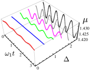
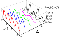
Figure 1: (a) Maximum fidelity between the instantaneous state of the system and a globally thermal state, plotted against the dimensionless evolution time and the (dimensionless) bias between the energies of the wells ΔΔ\Delta. (b) Corresponding estimate of the mean energy μ𝜇\mu of the target globally thermal state. In both panels, we have taken J=2𝐽2J=2, n¯1=n¯2/2=1subscript¯𝑛1subscript¯𝑛221\overline{n}_{1}=\overline{n}_{2}/2=1.

III Assessment of dynamical thermalisation

We shall start with the study of the unitary case. Dynamical thermalisation in closed-system dynamics is a topic of vast interest, which has recently attracted considerable attention at both the theoretical and experimental level Trotzky . Our approach is based on the assessment of the distance between the time-dependent state of the system and a generic (either global or local) thermal state. Quantitatively, as a measure of the distance between two states ρ1,2subscript𝜌12\rho_{1,2}, we use the Ulhmann fidelity uhlmann

F(ρ1,ρ2)=(Trρ1ρ2ρ1)2.𝐹subscript𝜌1subscript𝜌2superscriptTrsubscript𝜌1subscript𝜌2subscript𝜌12F(\rho_{1},\rho_{2})=\left({\rm Tr}\sqrt{\sqrt{\rho_{1}}\rho_{2}\sqrt{\rho_{1}}}\right)^{2}. (17)

For Gaussian states, it can be conveniently evaluated using the covariance matrices σ1,2subscript𝜎12\sigma_{1,2} associated to the states under scrutiny. The explicit formula, which has been recently reported in Ref. marian , reads

F(σ1,σ2)=4(x+x1)2det(σ1+σ1),𝐹subscript𝜎1subscript𝜎24superscript𝑥𝑥12detsubscript𝜎1subscript𝜎1F(\sigma_{1},\sigma_{2})=4\frac{(\sqrt{x}+\sqrt{x-1})^{2}}{\sqrt{{\rm det}(\sigma_{1}+\sigma_{1})}}, (18)

where Ω=i(σyσy)Ω𝑖direct-sumsubscript𝜎𝑦subscript𝜎𝑦\Omega=i(\sigma_{y}\oplus\sigma_{y}) is the two-mode symplectic matrix (σysubscript𝜎𝑦\sigma_{y} being the y𝑦y-Pauli matrix) and x=21+22+1/2𝑥2subscript12subscript212x=2\sqrt{{\cal I}_{1}}+2\sqrt{{\cal I}_{2}}+1/2 with

1=det(Ωσ1Ωσ1𝟙𝟜)16det(σ1+σ2),2=det(σ1+iΩ)det(σ2+iΩ)16det(σ1+σ2).formulae-sequencesubscript1detΩsubscript𝜎1Ωsubscript𝜎1subscript𝟙416detsubscript𝜎1subscript𝜎2subscript2detsubscript𝜎1𝑖Ωdetsubscript𝜎2𝑖Ω16detsubscript𝜎1subscript𝜎2{\cal I}_{1}=\frac{{\rm det}(\Omega\sigma_{1}\Omega\sigma_{1}-\openone_{4})}{16{\rm det}(\sigma_{1}+\sigma_{2})},~{}~{}{\cal I}_{2}=\frac{{\rm det}(\sigma_{1}+i\Omega){\rm det}(\sigma_{2}+i\Omega)}{16{\rm det}(\sigma_{1}+\sigma_{2})}. (19)

In our case we consider σ1=σu(t)subscript𝜎1subscript𝜎𝑢𝑡\sigma_{1}=\sigma_{u}(t) [cf. Eq. (11)] and σ2subscript𝜎2\sigma_{2} given by either σ2G=(2μ+1)𝟙𝟜subscriptsuperscript𝜎𝐺22𝜇1subscript𝟙4\sigma^{G}_{2}=(2\mu+1)\openone_{4}, i.e. the covariance matrix of a globally thermal state with mean number of excitations μ𝜇\mu, or σ2L=(2μ1+1)𝟙𝟚(𝟚μ𝟚+𝟙)𝟙𝟚subscriptsuperscript𝜎𝐿2direct-sum2subscript𝜇11subscript𝟙22subscript𝜇21subscript𝟙2\sigma^{L}_{2}=(2\mu_{1}+1)\openone_{2}\oplus(2\mu_{2}+1)\openone_{2}, which is the one associated with the tensor product of locally thermal states (each with mean number of excitations μjsubscript𝜇𝑗\mu_{j}). For clarity, we have indicated with 𝟙𝕟subscript𝟙𝕟\openone_{n} the identity matrix of dimension n𝑛n.

We present the case of global thermalisation first: after calculating the time behaviour of F(σu(t),σ2G)𝐹subscript𝜎𝑢𝑡subscriptsuperscript𝜎𝐺2F(\sigma_{u}(t),\sigma^{G}_{2}) for various choices of ΔΔ\Delta, we have numerically evaluated the value of μ𝜇\mu that achieves the maximum of F(σu(t),σ2G)𝐹subscript𝜎𝑢𝑡subscriptsuperscript𝜎𝐺2F(\sigma_{u}(t),\sigma^{G}_{2}). In Fig. 1 we show both such value and the corresponding estimate for μ𝜇\mu. The state fidelity remains evidently quite large, being only partially depleted by an increasing value of ΔΔ\Delta (the dependence on such parameter is quite non-trivial, given that for Δ=2.5Δ2.5\Delta=2.5, for instance, values very close to those associated with Δ=0Δ0\Delta=0 can be achieved, at suitable times in the evolution). However, while at small values of ΔΔ\Delta the target state changes very little with time, this is not the case for increasing bias: the value of μ𝜇\mu corresponding to a non-zero ΔΔ\Delta oscillates with a non-negligible amplitude as this parameter grows. In any case, perfect thermalisation is never achieved, a result that is strengthened by the analysis that we will report in the next Section.

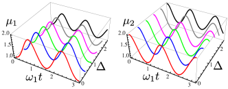
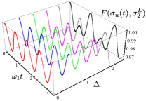
The situation is somehow different when locally thermal target states are considered [cf. Fig. 2]: besides the expected times at which a full period of the evolution is achieved, it is possible to identify instants of time at which the state of the double-well system is indeed very close to a locally thermal state (F(σu(t),σ2L)0.999𝐹subscript𝜎𝑢𝑡subscriptsuperscript𝜎𝐿20.999F(\sigma_{u}(t),\sigma^{L}_{2})\geq 0.999), which would suggest the occurrence of accidental dynamical thermalisation.

(a)
Refer to caption
(b)
                      (c)
Refer to caption

Figure 2: (a) Maximum fidelity between the instantaneous state of the system and a locally thermal state, plotted against the dimensionless evolution time and the (dimensionless) bias between the energies of the wells ΔΔ\Delta. (b) & (c) Estimate of the corresponding mean number of excitations μ1,2subscript𝜇12\mu_{1,2} of the target locally thermal state. In both panels, we have taken J=2𝐽2J=2, n¯1=n¯2/2=1subscript¯𝑛1subscript¯𝑛221\overline{n}_{1}=\overline{n}_{2}/2=1.

(a)
Refer to caption
(b)
Refer to caption

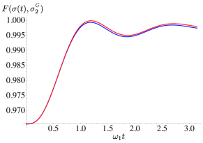
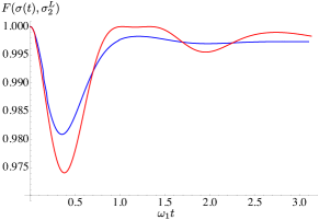
Figure 3: Open-system dynamics. (a) Fidelity with a globally thermal state for J=2𝐽2J=2, n¯1=1subscript¯𝑛11\overline{n}_{1}=1, n¯2=2subscript¯𝑛22\overline{n}_{2}=2, γ1/ω1=γ2/ω1=1subscript𝛾1subscript𝜔1subscript𝛾2subscript𝜔11\gamma_{1}/\omega_{1}=\gamma_{2}/\omega_{1}=1. We have taken Δ=0Δ0\Delta=0 (blue line) and Δ=0.5Δ0.5\Delta=0.5 (red line). (b) Fidelity with locally thermal states for J=2𝐽2J=2, n¯1=1subscript¯𝑛11\overline{n}_{1}=1, n¯2=2subscript¯𝑛22\overline{n}_{2}=2, and Δ=0Δ0\Delta=0. We have taken γ1/ω1=γ2/ω1=1subscript𝛾1subscript𝜔1subscript𝛾2subscript𝜔11\gamma_{1}/\omega_{1}=\gamma_{2}/\omega_{1}=1 (red line) and γ1/ω1=1subscript𝛾1subscript𝜔11\gamma_{1}/\omega_{1}=1 with γ2/ω1=3subscript𝛾2subscript𝜔13\gamma_{2}/\omega_{1}=3 (blue line).

In the open-system dynamics case, a similar calculation allows us to evaluate the fidelity with both a globally thermal and locally thermal state as shown in Fig. 3, which studies the effects of both the energy bias [panel (a)] and a difference in the damping rates of the two wells [panel (b)]. Quite evidently, both effects spoil the state fidelity, which however achieves values that are either precisely 1 or very close to it. Indeed, focusing on the unbiased case with Δ=0Δ0\Delta=0 and γ1=γ2subscript𝛾1subscript𝛾2\gamma_{1}=\gamma_{2}, we know that the solution is given in the form of Eq. (15). Moreover, the off-diagonal block matrix 𝐜𝐜\bf{c} turns out to be anti-diagonal with entries equal in modulus but opposite in sign. Therefore, in order to determine if the system has accidentally thermalised, we need only to determine if, at some value of t𝑡t, these entries are identically zero. After some manipulation, this condition reduces to the transcendental equation

eγ1t=cos(2𝒥t)2𝒥γ1sin(2𝒥t).superscript𝑒subscript𝛾1𝑡2𝒥𝑡2𝒥subscript𝛾12𝒥𝑡e^{\gamma_{1}t}=\cos\left(2{\cal J}t\right)-\frac{2{\cal J}}{\gamma_{1}}\sin\left(2{\cal J}t\right). (20)

Interestingly, this ‘accidental’ thermalisation is independent of the temperature of either well and only concerned with the tunnelling strength and the damping rate. For the same parameters taken to obtain the red curve in Fig. 3 (b), we find Eq. (20) has two solutions: t1.03438ω11similar-to𝑡1.03438superscriptsubscript𝜔11t\sim 1.03438\omega_{1}^{-1} and t1.33749ω11similar-to𝑡1.33749superscriptsubscript𝜔11t\sim 1.33749\omega_{1}^{-1}, clearly corresponding to the two instances of local thermalisation in Fig. 3 (b). Furthermore, we find the thermal occupation numbers of the wells at the first instance of thermalisation are n¯1=1.597subscript¯𝑛11.597\overline{n}_{1}=1.597 and n¯2=1.403subscript¯𝑛21.403\overline{n}_{2}=1.403, and at the second are n¯1=1.422subscript¯𝑛11.422\overline{n}_{1}=1.422 and n¯2=1.578subscript¯𝑛21.578\overline{n}_{2}=1.578, thus suggesting that the two instants of accidental thermalisation correspond to an almost swap of the two local thermal states. Increasing J𝐽J leads to more instances of accidental thermalisation occurring before the system equilibrates to its steady state.

IV Assessment of the non-classical nature of the state of the system.

Values of fidelity so close to unity should not lead to misinterpretation of the actual nature of the state of the two-well system. In fact, any assessment of fidelity should be accompanied by the study of problem-specific figures of merit able to provide a more fine-grained characterisation of the state at hand. For the sake of a study on thermalisation, a significant class of such quantifiers is embodied by measures of quantum correlations.

In this respect, it is important here to assess the role, if any, various forms of quantum correlations play in the dynamics highlighted above. It is quickly confirmed that, as anticipated before, the system never becomes entangled. While this is expected in light of the nature of the interaction and initial state being considered, nothing prevents the settlement of weaker forms of quantum correlations, such as quantum discord (QD) discordreview . QD is the difference between two classically equivalent definitions of mutual information when applied to a quantum system zurek ; vedral . A non-zero degree of QD implies that, in a bipartite system composed of parties A and B, information can be gathered on system A by interrogating party B. For Gaussian states, QD is captured by the Gaussian quantum discord adesso ; olivares ; paris , which entails that the interrogation of B only involves Gaussian measurements. For a generic covariance matrix S=(ACCB)𝑆𝐴𝐶superscript𝐶top𝐵S=\left(\begin{array}[]{cc}A&C\\ C^{\top}&B\end{array}\right), QD is then defined following Ref. adesso (to be consistent with the definition of the vacuum state used throughout)

𝒟G=h(I1)h(d)h(d+)+h(Emin),subscript𝒟𝐺subscript𝐼1subscript𝑑subscript𝑑superscript𝐸min\mathcal{D}_{G}=h\left(\sqrt{I_{1}}\right)-h\left(d_{-}\right)-h\left(d_{+}\right)+h\left(\sqrt{E^{\text{min}}}\right), (21)

with

Emin={1(I11)2[2I32+(I11)(I4I2)+2|I3|I32+(I11)(I4I2)]for(I4I1I2)2I32(I2+I4)(I1+1),12I1[I1I2I32+I4I34+(I4I1I2)22I32(I1I2+I4)]otherwise,superscript𝐸mincases1superscriptsubscript𝐼112delimited-[]2superscriptsubscript𝐼32subscript𝐼11subscript𝐼4subscript𝐼22subscript𝐼3superscriptsubscript𝐼32subscript𝐼11subscript𝐼4subscript𝐼2forsuperscriptsubscript𝐼4subscript𝐼1subscript𝐼22superscriptsubscript𝐼32subscript𝐼2subscript𝐼4subscript𝐼11otherwiseotherwiseotherwise12subscript𝐼1delimited-[]subscript𝐼1subscript𝐼2superscriptsubscript𝐼32subscript𝐼4superscriptsubscript𝐼34superscriptsubscript𝐼4subscript𝐼1subscript𝐼222superscriptsubscript𝐼32subscript𝐼1subscript𝐼2subscript𝐼4otherwiseotherwiseE^{\text{min}}=\begin{cases}\dfrac{1}{(I_{1}-1)^{2}}\left[{2I_{3}^{2}+(I_{1}-1)(I_{4}-I_{2})+2|I_{3}|\sqrt{I_{3}^{2}+(I_{1}-1)(I_{4}-I_{2})}}\right]\quad\text{for}~{}(I_{4}-I_{1}I_{2})^{2}\leq I_{3}^{2}(I_{2}+I_{4})(I_{1}+1),\\ ~{}~{}\\ \dfrac{1}{2I_{1}}\left[{I_{1}I_{2}-I_{3}^{2}+I_{4}-\sqrt{I_{3}^{4}+(I_{4}-I_{1}I_{2})^{2}-2I_{3}^{2}(I_{1}I_{2}+I_{4})}}\right]\quad\text{otherwise},\end{cases}

where

h(x)=(x+12)log(x+12)(x12)log(x12),𝑥𝑥12𝑥12𝑥12𝑥12\displaystyle h(x)=\left(\frac{x+1}{2}\right)\log\left(\frac{x+1}{2}\right)-\left(\frac{x-1}{2}\right)\log\left(\frac{x-1}{2}\right), (22)
d±2=12(Λ±Λ24I4),superscriptsubscript𝑑plus-or-minus212plus-or-minusΛsuperscriptΛ24subscript𝐼4\displaystyle d_{\pm}^{2}=\frac{1}{2}\left(\Lambda\pm\sqrt{\Lambda^{2}-4I_{4}}\right),
Λ=I1+I2+2I3,Λsubscript𝐼1subscript𝐼22subscript𝐼3\displaystyle\Lambda=I_{1}+I_{2}+2I_{3},

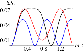
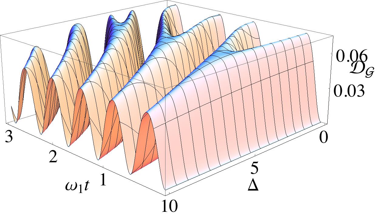
and I1=detAsubscript𝐼1𝐴I_{1}=\det A, I2=detBsubscript𝐼2𝐵I_{2}=\det B, I3=detCsubscript𝐼3𝐶I_{3}=\det C, and I4=detSsubscript𝐼4𝑆I_{4}=\det S. In Fig. 4 (a) we study QD against the energy bias for the case of the unitary solution Eq. (11). Intuitively we would expect that for Δ=0Δ0\Delta=0, owing to the full symmetry enforced in the system, QD will be maximised. This is indeed the case, as it can be seen in Fig. 4 (a). However, an interesting feature appears as we increase the bias. At Δ/J2.5similar-toΔ𝐽2.5\Delta/J\sim 2.5, n¯1=1subscript¯𝑛11\overline{n}_{1}=1, and n¯2=5subscript¯𝑛25\overline{n}_{2}=5, QD exhibits a plateau, which implies the existence of an ‘optimal’ value of the bias, dependent on the temperature difference, that helps amplify the non-classicality of the system. Further increase of ΔΔ\Delta pushes the systems too far off resonance, and the coherence decays. In Fig. 4 (b) we examine this phenomenon closer, for a fixed temperature difference and small biasing, Δ/J=1,Δ𝐽1\Delta/J=1, (red), we see the oscillatory behaviour changes and the first zero-point is lifted. At the optimal value of ΔΔ\Delta (solid black) the plateau is clearly evident. When we increase the bias further, we see the decay in the non-classicality, as well as a change in the periodicity of the system.

(a)
Refer to caption
(b)

Refer to caption

Figure 4: (a) Discord versus bias and evolution time for the case of closed-system dynamics. We have taken n¯1=1subscript¯𝑛11\overline{n}_{1}=1, n¯2=5subscript¯𝑛25\overline{n}_{2}=5, J=2𝐽2J=2. (b) Behaviour of quantum discord in the open-system scenario for n¯1=1subscript¯𝑛11\overline{n}_{1}=1, n¯2=5subscript¯𝑛25\overline{n}_{2}=5, J=2𝐽2J=2 and the bias choices Δ=1Δ1\Delta=1 (red curve), 5 (black curve), and 10 (blue curve).

(a)
Refer to caption
(b)
Refer to caption
(c)
Refer to caption

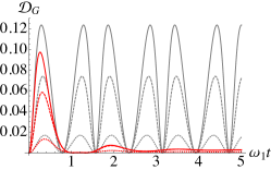
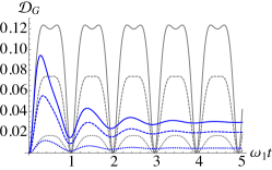
Figure 5: (a) Dynamical discord for the unitary (gray) and dissipative (red) cases. For both J=2𝐽2J=2, n¯1=1subscript¯𝑛11\overline{n}_{1}=1, and n¯2=subscript¯𝑛2absent\overline{n}_{2}= 2 (dotted), 5 (dashed), and 10 (solid). For all the dissipative cases γ1/ω1=γ2/ω1=1subscript𝛾1subscript𝜔1subscript𝛾2subscript𝜔11\gamma_{1}/\omega_{1}=\gamma_{2}/\omega_{1}=1. (b) As for panel (a) but with the optimal bias (for n¯1=1subscript¯𝑛11\overline{n}_{1}=1, n¯2=5subscript¯𝑛25\overline{n}_{2}=5) between the wells, Δ=5Δ5\Delta=5. (c) Dissipative dynamical discord J=2𝐽2J=2, Δ=4Δ4\Delta=4, γ1/ω1=γ2/ω1=1subscript𝛾1subscript𝜔1subscript𝛾2subscript𝜔11\gamma_{1}/\omega_{1}=\gamma_{2}/\omega_{1}=1, n¯1=1subscript¯𝑛11\overline{n}_{1}=1, and n¯2=2subscript¯𝑛22\overline{n}_{2}=2, with self interaction term U=0𝑈0U=0, U=1𝑈1U=1 and U=3𝑈3U=3 going from top to bottom.

Turning our attention to the dissipative case, in Fig. 5 we compare the unitary dynamics with the dissipative case for unbiased wells [panel (a)], and biased ones [panel (b)] at various differences in temperature. For unbiased wells, we see dissipation quickly suppresses the the oscillations and we reach a steady state with non-vanishing QD. As we increase the temperature between the wells we see an increase in the QD for the unitary case and the steady state QD is larger for increasing temperature difference. When we bias the wells, taking Δ/J=2.5Δ𝐽2.5\Delta/J=2.5 for all temperature differences, we see the dissipative dynamics clearly show the enhanced non-classicality. While the time to reach equilibrium appears unaffected, the steady state is significantly more non-classical than in the unbiased situation. This may imply that in this situation the non-classicality plays no role in reaching equilibrium. In Fig. 5 (c) we examine the effect that self-interaction has on the dynamics of nonclassicality. In order to do so, we compute the Gaussian discord of the hypothetical Gaussian state having, as covariance matrix, the one achieved by calculating the entries σijsubscript𝜎𝑖𝑗\sigma_{ij} over the non-Gaussian state resulting from a chosen non-zero values of U𝑈U. Evidently the larger the self interaction, the more self ordered each well becomes, diminishing the effect of the tunnelling and reducing the amount of nonclassicality present. Also we see the system tends to equilibrate faster.

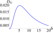
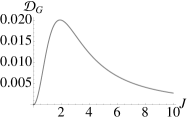
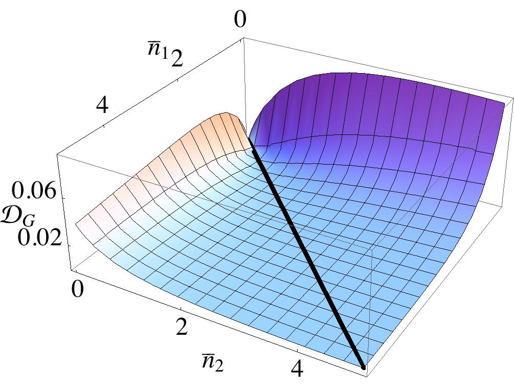
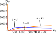
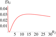
The nonclassicality of the steady state is delicately dependent on the temperature difference, as well as the tunneling rate and the bias. In Fig. 6 we examine this behaviour closer, fixing n¯1subscript¯𝑛1\overline{n}_{1} and γ1/ω1=γ2/ω1=1subscript𝛾1subscript𝜔1subscript𝛾2subscript𝜔11\gamma_{1}/\omega_{1}=\gamma_{2}/\omega_{1}=1 with J=2𝐽2J=2 and Δ=5Δ5\Delta=5. The only conditions for which the system does not exhibit nonclassical correlations is the trivial one of n¯2=n¯1subscript¯𝑛2subscript¯𝑛1\overline{n}_{2}=\overline{n}_{1}. As we increase the temperature imbalance we see that QD increases to a maximum value before slowly decaying [cf. Figs. 6 (a) and (e)]. If we fix the temperature difference such that n¯1=1subscript¯𝑛11\overline{n}_{1}=1 and n¯2=5subscript¯𝑛25\overline{n}_{2}=5, we see in panels (b) and (c) that there are optimal values of the remaining parameters that give the largest value of discord. While the reservoirs have been kept at moderately low energies, in panel (f) we significantly increase both n¯1subscript¯𝑛1\overline{n}_{1} and n¯2subscript¯𝑛2\overline{n}_{2} and see that large values of QD can still be achieved. An unbiased configuration leads to values of discord of the order of 105superscript10510^{-5}. Increasing the bias, such values are raised by up to one order of magnitude.

(a)                               (b)
Refer to caption
 Refer to caption
(c)                               (d)
Refer to caption
 Refer to caption
(e)                               (f)
Refer to caption
 Refer to caption

Figure 6: Steady-state discord between the two wells for γ1/ω1=γ2/ω1=1subscript𝛾1subscript𝜔1subscript𝛾2subscript𝜔11\gamma_{1}/\omega_{1}=\gamma_{2}/\omega_{1}=1, and n¯1=1subscript¯𝑛11\overline{n}_{1}=1. (a) Plotted against n¯2subscript¯𝑛2\overline{n}_{2} for J=2𝐽2J=2, Δ=5Δ5\Delta=5. (b) Against ΔΔ\Delta for J=2𝐽2J=2 and n¯2=5subscript¯𝑛25\overline{n}_{2}=5. (c) Against J𝐽J for n¯2=5subscript¯𝑛25\overline{n}_{2}=5 and Δ=5Δ5\Delta=5. (d) Maximum discord attainable for a given value of n¯2subscript¯𝑛2\overline{n}_{2} found by optimising with respect to both ΔΔ\Delta and J𝐽J when n¯1=1subscript¯𝑛11\overline{n}_{1}=1 and γ1/ω1=γ2/ω1=1subscript𝛾1subscript𝜔1subscript𝛾2subscript𝜔11\gamma_{1}/\omega_{1}=\gamma_{2}/\omega_{1}=1. (e) Steady-state discord studied against both n¯1subscript¯𝑛1\overline{n}_{1} and n¯2subscript¯𝑛2\overline{n}_{2} when J=2𝐽2J=2, Δ=5Δ5\Delta=5, and γ1/ω1=γ2/ω1=1subscript𝛾1subscript𝜔1subscript𝛾2subscript𝜔11\gamma_{1}/\omega_{1}=\gamma_{2}/\omega_{1}=1. The black line shows that 𝒟Gsubscript𝒟𝐺\mathcal{D}_{G} is identically null only when n¯1=n¯2subscript¯𝑛1subscript¯𝑛2\overline{n}_{1}=\overline{n}_{2}. (f) Steady-state discord against n¯2subscript¯𝑛2\overline{n}_{2} for n¯1=100subscript¯𝑛1100\overline{n}_{1}=100 with J=2𝐽2J=2, γ1/ω1=γ2/ω1=1subscript𝛾1subscript𝜔1subscript𝛾2subscript𝜔11\gamma_{1}/\omega_{1}=\gamma_{2}/\omega_{1}=1.

V Dynamics of the energy flux between the wells

It is important to gather insight into the details of the exchange of energy between the wells of the system, which is at the basis of the process of quasi-thermalisation highlighted so far and takes place in two forms: an exchange of particles between the wells and a similar process occurring at the interface between the double-well system and the reservoirs. The aim of this section is to identify the contribution coming from both such fluxes. We are thus interested in quantifying the flux into/from well j=1,2𝑗12j=1,2, which we label as 𝒬˙jsubscript˙𝒬𝑗\dot{\mathcal{Q}}_{j} , and the total flux 𝒬˙totsubscript˙𝒬𝑡𝑜𝑡\dot{\mathcal{Q}}_{tot}. These are given by the quantities

𝒬˙tot=Tr[^tϱ],𝒬˙j=Tr[^jtϱj],(j=1,2),formulae-sequencesubscript˙𝒬𝑡𝑜𝑡Trdelimited-[]^subscript𝑡italic-ϱsubscript˙𝒬𝑗Trdelimited-[]subscript^𝑗subscript𝑡subscriptitalic-ϱ𝑗𝑗12\dot{\mathcal{Q}}_{tot}=\text{Tr}[\hat{\cal H}\partial_{t}\varrho],\qquad\dot{\mathcal{Q}}_{j}=\text{Tr}[\hat{\cal H}_{j}\partial_{t}\varrho_{j}],~{}~{}(j=1,2),\\ (23)

where ^j=ωj(a^ja^j+1/2)subscript^𝑗subscript𝜔𝑗subscriptsuperscript^𝑎𝑗subscript^𝑎𝑗12\hat{\cal H}_{j}=\omega_{j}(\hat{a}^{\dagger}_{j}\hat{a}_{j}+1/2) is the free evolution of a single well and ϱjsubscriptitalic-ϱ𝑗\varrho_{j} is the density matrix of well j𝑗j. Conveniently, these quantities can be directly evaluated from the covariance matrix (and we will assume both wells to have the same damping rate, i.e. γ1/ω1=γ2/ω1=γsubscript𝛾1subscript𝜔1subscript𝛾2subscript𝜔1𝛾\gamma_{1}/\omega_{1}=\gamma_{2}/\omega_{1}=\gamma). We find

𝒬˙1=eγt[2J2(1+Δ)(n¯2n¯1)4J2+Δ2sin(4J2+Δ2t)],subscript˙𝒬1superscript𝑒𝛾𝑡delimited-[]2superscript𝐽21Δsubscript¯𝑛2subscript¯𝑛14superscript𝐽2superscriptΔ24superscript𝐽2superscriptΔ2𝑡\displaystyle\dot{\mathcal{Q}}_{1}=e^{-\gamma t}\left[\frac{2J^{2}(1+\Delta)(\overline{n}_{2}-\overline{n}_{1})}{\sqrt{4J^{2}+\Delta^{2}}}\sin\left(\sqrt{4J^{2}+\Delta^{2}}t\right)\right], (24)
𝒬˙2=(1+Δ)𝒬˙1,𝒬˙tot=0.formulae-sequencesubscript˙𝒬21Δsubscript˙𝒬1subscript˙𝒬𝑡𝑜𝑡0\displaystyle\dot{\mathcal{Q}}_{2}=-(1+\Delta)\dot{\mathcal{Q}}_{1},\qquad\dot{\mathcal{Q}}_{tot}=0.

From here it is easy to confirm that 𝒬˙1/ω1=𝒬˙2/ω2subscript˙𝒬1subscript𝜔1subscript˙𝒬2subscript𝜔2{\dot{\mathcal{Q}}_{1}}/{\omega_{1}}=-{\dot{\mathcal{Q}}_{2}}/{\omega_{2}} and clearly taking γ=0𝛾0\gamma=0 or Δ=0Δ0\Delta=0 recovers the unitary and unbiased limits respectively. However, this behaviour is only for the special case of the wells initially being thermalised with their baths, while taking a different initial state this behaviour no longer holds. Indeed, what is special about our initial state is that it conserves the total energy of the system. This is readily seen given that 𝒬˙tot=0subscript˙𝒬𝑡𝑜𝑡0\dot{\mathcal{Q}}_{tot}=0 and it is easy to confirm that

𝒬tot=1+Δ2+n¯1+(1+Δ)n¯2,subscript𝒬𝑡𝑜𝑡1Δ2subscript¯𝑛11Δsubscript¯𝑛2\mathcal{Q}_{tot}=1+\frac{\Delta}{2}+\overline{n}_{1}+(1+\Delta)\overline{n}_{2}, (25)

for all t𝑡t and J𝐽J. Of course, the energy of the individual wells changes dynamically (until settling into the same steady state).

We can gain further insight into the reason for this by examining closer the quantity we are calculating, i.e.

𝒬˙totsubscript˙𝒬𝑡𝑜𝑡\displaystyle\dot{\mathcal{Q}}_{tot} =Tr[^tϱ]absentTrdelimited-[]^subscript𝑡italic-ϱ\displaystyle=\text{Tr}[\hat{\mathcal{H}}\partial_{t}\varrho]
=Tr[^(i[^,ϱ]+i=12i(ϱ))]absentTrdelimited-[]^𝑖^italic-ϱsuperscriptsubscript𝑖12subscript𝑖italic-ϱ\displaystyle=\text{Tr}\left[\hat{\mathcal{H}}\left(-i[\hat{\mathcal{H}},\varrho]+\sum_{i=1}^{2}\mathcal{L}_{i}(\varrho)\right)\right]
=iTr[^(^ϱϱ^)]+Tr[^i=12i(ϱ)]absent𝑖Trdelimited-[]^^italic-ϱitalic-ϱ^Trdelimited-[]^superscriptsubscript𝑖12subscript𝑖italic-ϱ\displaystyle=-i\text{Tr}\left[\hat{\mathcal{H}}\left(\hat{\mathcal{H}}\varrho-\varrho\hat{\mathcal{H}}\right)\right]+\text{Tr}\left[\hat{\mathcal{H}}\sum_{i=1}^{2}\mathcal{L}_{i}(\varrho)\right]
=Tr[^i=12i(ϱ)].absentTrdelimited-[]^superscriptsubscript𝑖12subscript𝑖italic-ϱ\displaystyle=\text{Tr}\left[\hat{\mathcal{H}}\sum_{i=1}^{2}\mathcal{L}_{i}(\varrho)\right].

The tunnelling term in Eq. (1) commutes with isubscript𝑖\mathcal{L}_{i}, and when U=0𝑈0U=0 the only contribution to the total flux is from the free evolution of each well. Therefore we are interested in calculating

𝒬˙tot=Tr[(n¯1+n¯2)1(ϱ)]+Tr[(n¯1+n¯2)2(ϱ)].subscript˙𝒬𝑡𝑜𝑡Trdelimited-[]subscript¯𝑛1subscript¯𝑛2subscript1italic-ϱTrdelimited-[]subscript¯𝑛1subscript¯𝑛2subscript2italic-ϱ\dot{\mathcal{Q}}_{tot}=\text{Tr}\left[\left(\overline{n}_{1}+\overline{n}_{2}\right)\mathcal{L}_{1}(\varrho)\right]+\text{Tr}\left[\left(\overline{n}_{1}+\overline{n}_{2}\right)\mathcal{L}_{2}(\varrho)\right]. (26)

In a tedious but otherwise straightforward calculation, we can explicitly evaluate this expression when assuming the special initial condition ϱ=eβ1^1𝒵1eβ2^2𝒵2italic-ϱtensor-productsuperscript𝑒subscript𝛽1subscript^1subscript𝒵1superscript𝑒subscript𝛽2subscript^2subscript𝒵2\varrho=\frac{e^{-\beta_{1}\hat{\cal H}_{1}}}{\mathcal{Z}_{1}}\otimes\frac{e^{-\beta_{2}\hat{\cal H}_{2}}}{\mathcal{Z}_{2}}, with 𝒵j=Tr[eβj^j]subscript𝒵𝑗Trdelimited-[]superscript𝑒subscript𝛽𝑗subscript^𝑗{\cal Z}_{j}=\text{Tr}[e^{-\beta_{j}\hat{\cal H}_{j}}]. We find that both the terms entering Eq. (26) are identically zero, thus showing that, in the U=0𝑈0U=0 case, the net heat flux is null due to two special circumstances: on one hand our chosen initial state, on the other hand the tunnelling term commutes with the super operators.

(a)
Refer to caption
(b)
Refer to caption
(c)
Refer to caption

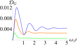
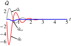
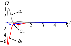
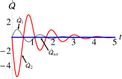
Figure 7: Steady-state discord between the two wells. In all panels J=2,γ=1,n¯1=1,n¯2=2,Δ=4.formulae-sequence𝐽2formulae-sequence𝛾1formulae-sequencesubscript¯𝑛11formulae-sequencesubscript¯𝑛22Δ4J=2,~{}\gamma=1,~{}\overline{n}_{1}=1,~{}\overline{n}_{2}=2,~{}\Delta=4. Red Line: hotter well (well 2), gray line cooler well (well 1), and blue the total flux. With (a) U=0.𝑈0U=0. (b) U=1.𝑈1U=1. (c) U=3.𝑈3U=3.

In Fig. 7 (a) we show the dynamics of the various energy fluxes given in Eq. (23). We notice how the flux into the cooler well is proportional to the flux out of the hotter well, which results in a null net flux. Needless to say, the single-well fluxes only account for the net intake/outtake of particles for one of the wells and do not provide information on the actual balance between the contribution due to the coupling to the reservoir and that due to the coherent inter-well interaction.

We can study the intermediate dynamical regime where the self-interaction is non-zero and comparable with the tunnelling by numerically solving Eq. (2) and examining the behaviour of the heat fluxes, of which we illustrate some examples in Fig. 7 (b) and (c) [we refer to the caption for an account of the parameters used in the simulations]. The total flux is now non-zero, and the energy is not conserved. However, the average occupation number is conserved, i.e. a^1a^1/ω1=a^2a^2/ω2delimited-⟨⟩superscriptsubscript^𝑎1subscript^𝑎1subscript𝜔1delimited-⟨⟩superscriptsubscript^𝑎2subscript^𝑎2subscript𝜔2{\langle\hat{a}_{1}^{\dagger}\hat{a}_{1}\rangle}/{\omega_{1}}=-{\langle\hat{a}_{2}^{\dagger}\hat{a}_{2}\rangle}/{\omega_{2}}, which follows directly from the previous arguments.

VI Discussion

The analysis above shows that neither global nor local thermalisation with the reservoirs is achieved. The fidelity between the density matrices of the time-evolved state and the target thermal one (whether globally or locally) connects the closeness of the populations of the energy levels of the former to the statistics of the latter. However, the interaction between the wells establishes strong quantum coherence between the particles of the systems, which in turn results in the generation of a substantive degree of quantum correlations, albeit of a nature weaker than entanglement, which prevents the thermal character of the resulting state.

The analysis reported here also has the merit of providing rather deep insight into the phenomenology of quantum correlations between the wells. We have qualitatively and quantitatively examined the dynamics and steady state of a BEC loaded into a double well potential. While the wells remain separable at all times, thus sharing no entanglement, by exploring the behaviour of the quantum discord we find the system to be always non-classical, except under trivial, uninteresting conditions. Furthermore, the degree of nonclassicality of the system is dependent on the energy bias between the two wells. For identical wells, a significant amount of QD is possible, provided that a large temperature imbalance is established. Such nonclassicality can be greatly enhanced by taking a suitable value of tunnelling, which must be a function of the given bias. The transfer of heat in the system is equally complex.

VII Methods

Differential Equations. Here we provide the complete set of differential equations that describe the dissipative dynamics considered throughout.

ty1=Jz2γ12y1+ω1z1,ty2=Jz1γ22y2+ω2z2,tz1=Jy2γ12z1ω1y1,tz2=Jy1γ22z2ω2y2,tσ1x=γ1+2n¯1γ12Jσ12xpγ1σ1x+2ω1σ1xp,tσ2x=γ2+2n¯2γ22Jσ12pxγ2σ2x+2ω2σ2xp,tσ1p=γ1+2n¯1γ1+2Jσ12pxγ1σ1p2ω1σ1xp,tσ2p=γ2+2n¯2γ2+2Jσ12xpγ2σ2p2ω2σ2xp,tσ1xp=J(σ12xσ12p)γ1σ1xpω1(σ1xσ1p),tσ2xp=J(σ12xσ12p)γ2σ2xpω1(σ2xσ2p),tσ12x=J(σ1xp+σ2xp)γ1+γ22σ12x+ω1σ12px+ω2σ12xp,tσ12p=J(σ1xp+σ2xp)γ1+γ22σ12pω1σ12xpω2σ12px,tσ12xp=J(σ1xσ2p)γ1+γ22σ12xp+ω1σ12pω2σ12x,tσ12px=J(σ2xσ1p)γ1+γ22σ12pxω1σ12x+ω2σ12p.matrixformulae-sequencesubscript𝑡subscript𝑦1𝐽subscript𝑧2subscript𝛾12subscript𝑦1subscript𝜔1subscript𝑧1subscript𝑡subscript𝑦2𝐽subscript𝑧1subscript𝛾22subscript𝑦2subscript𝜔2subscript𝑧2formulae-sequencesubscript𝑡subscript𝑧1𝐽subscript𝑦2subscript𝛾12subscript𝑧1subscript𝜔1subscript𝑦1subscript𝑡subscript𝑧2𝐽subscript𝑦1subscript𝛾22subscript𝑧2subscript𝜔2subscript𝑦2subscript𝑡superscriptsubscript𝜎1𝑥subscript𝛾12subscript¯𝑛1subscript𝛾12𝐽superscriptsubscript𝜎12𝑥𝑝subscript𝛾1superscriptsubscript𝜎1𝑥2subscript𝜔1superscriptsubscript𝜎1𝑥𝑝subscript𝑡superscriptsubscript𝜎2𝑥subscript𝛾22subscript¯𝑛2subscript𝛾22𝐽superscriptsubscript𝜎12𝑝𝑥subscript𝛾2superscriptsubscript𝜎2𝑥2subscript𝜔2superscriptsubscript𝜎2𝑥𝑝subscript𝑡superscriptsubscript𝜎1𝑝subscript𝛾12subscript¯𝑛1subscript𝛾12𝐽superscriptsubscript𝜎12𝑝𝑥subscript𝛾1superscriptsubscript𝜎1𝑝2subscript𝜔1superscriptsubscript𝜎1𝑥𝑝subscript𝑡superscriptsubscript𝜎2𝑝subscript𝛾22subscript¯𝑛2subscript𝛾22𝐽superscriptsubscript𝜎12𝑥𝑝subscript𝛾2superscriptsubscript𝜎2𝑝2subscript𝜔2superscriptsubscript𝜎2𝑥𝑝subscript𝑡superscriptsubscript𝜎1𝑥𝑝𝐽superscriptsubscript𝜎12𝑥superscriptsubscript𝜎12𝑝subscript𝛾1superscriptsubscript𝜎1𝑥𝑝subscript𝜔1superscriptsubscript𝜎1𝑥superscriptsubscript𝜎1𝑝subscript𝑡superscriptsubscript𝜎2𝑥𝑝𝐽superscriptsubscript𝜎12𝑥superscriptsubscript𝜎12𝑝subscript𝛾2superscriptsubscript𝜎2𝑥𝑝subscript𝜔1superscriptsubscript𝜎2𝑥superscriptsubscript𝜎2𝑝subscript𝑡superscriptsubscript𝜎12𝑥𝐽superscriptsubscript𝜎1𝑥𝑝superscriptsubscript𝜎2𝑥𝑝subscript𝛾1subscript𝛾22superscriptsubscript𝜎12𝑥subscript𝜔1superscriptsubscript𝜎12𝑝𝑥subscript𝜔2superscriptsubscript𝜎12𝑥𝑝subscript𝑡superscriptsubscript𝜎12𝑝𝐽superscriptsubscript𝜎1𝑥𝑝superscriptsubscript𝜎2𝑥𝑝subscript𝛾1subscript𝛾22superscriptsubscript𝜎12𝑝subscript𝜔1superscriptsubscript𝜎12𝑥𝑝subscript𝜔2superscriptsubscript𝜎12𝑝𝑥subscript𝑡superscriptsubscript𝜎12𝑥𝑝𝐽superscriptsubscript𝜎1𝑥superscriptsubscript𝜎2𝑝subscript𝛾1subscript𝛾22superscriptsubscript𝜎12𝑥𝑝subscript𝜔1superscriptsubscript𝜎12𝑝subscript𝜔2superscriptsubscript𝜎12𝑥subscript𝑡superscriptsubscript𝜎12𝑝𝑥𝐽superscriptsubscript𝜎2𝑥superscriptsubscript𝜎1𝑝subscript𝛾1subscript𝛾22superscriptsubscript𝜎12𝑝𝑥subscript𝜔1superscriptsubscript𝜎12𝑥subscript𝜔2superscriptsubscript𝜎12𝑝\begin{matrix}\partial_{t}y_{1}=-Jz_{2}-\frac{\gamma_{1}}{2}y_{1}+\omega_{1}z_{1},\quad\partial_{t}y_{2}=-Jz_{1}-\frac{\gamma_{2}}{2}y_{2}+\omega_{2}z_{2},&\partial_{t}z_{1}=Jy_{2}-\frac{\gamma_{1}}{2}z_{1}-\omega_{1}y_{1},\quad\partial_{t}z_{2}=Jy_{1}-\frac{\gamma_{2}}{2}z_{2}-\omega_{2}y_{2},\\ \partial_{t}\sigma_{1}^{x}=\gamma_{1}+2\overline{n}_{1}\gamma_{1}-2J\sigma_{12}^{xp}-\gamma_{1}\sigma_{1}^{x}+2\omega_{1}\sigma_{1}^{xp},&\partial_{t}\sigma_{2}^{x}=\gamma_{2}+2\overline{n}_{2}\gamma_{2}-2J\sigma_{12}^{px}-\gamma_{2}\sigma_{2}^{x}+2\omega_{2}\sigma_{2}^{xp},\\ \partial_{t}\sigma_{1}^{p}=\gamma_{1}+2\overline{n}_{1}\gamma_{1}+2J\sigma_{12}^{px}-\gamma_{1}\sigma_{1}^{p}-2\omega_{1}\sigma_{1}^{xp},&\partial_{t}\sigma_{2}^{p}=\gamma_{2}+2\overline{n}_{2}\gamma_{2}+2J\sigma_{12}^{xp}-\gamma_{2}\sigma_{2}^{p}-2\omega_{2}\sigma_{2}^{xp},\\ \partial_{t}\sigma_{1}^{xp}=J\left(\sigma_{12}^{x}-\sigma_{12}^{p}\right)-\gamma_{1}\sigma_{1}^{xp}-\omega_{1}\left(\sigma_{1}^{x}-\sigma_{1}^{p}\right),&\partial_{t}\sigma_{2}^{xp}=J\left(\sigma_{12}^{x}-\sigma_{12}^{p}\right)-\gamma_{2}\sigma_{2}^{xp}-\omega_{1}\left(\sigma_{2}^{x}-\sigma_{2}^{p}\right),\\ \partial_{t}\sigma_{12}^{x}=-J\left(\sigma_{1}^{xp}+\sigma_{2}^{xp}\right)-\frac{\gamma_{1}+\gamma_{2}}{2}\sigma_{12}^{x}+\omega_{1}\sigma_{12}^{px}+\omega_{2}\sigma_{12}^{xp},&\partial_{t}\sigma_{12}^{p}=J\left(\sigma_{1}^{xp}+\sigma_{2}^{xp}\right)-\frac{\gamma_{1}+\gamma_{2}}{2}\sigma_{12}^{p}-\omega_{1}\sigma_{12}^{xp}-\omega_{2}\sigma_{12}^{px},\\ \partial_{t}\sigma_{12}^{xp}=J\left(\sigma_{1}^{x}-\sigma_{2}^{p}\right)-\frac{\gamma_{1}+\gamma_{2}}{2}\sigma_{12}^{xp}+\omega_{1}\sigma_{12}^{p}-\omega_{2}\sigma_{12}^{x},&\partial_{t}\sigma_{12}^{px}=J\left(\sigma_{2}^{x}-\sigma_{1}^{p}\right)-\frac{\gamma_{1}+\gamma_{2}}{2}\sigma_{12}^{px}-\omega_{1}\sigma_{12}^{x}+\omega_{2}\sigma_{12}^{p}.\end{matrix} (27)

Discussions on self interaction dominated limit. While the main analysis treated the tunnelling dominated regime, the opposite extreme is determined setting J=0𝐽0J=0 and exploring the situation where self-interaction dominates. In this instance, the two wells are completely decoupled from one another. We can directly solve Eq. (2) by projecting onto the number states |nket𝑛\left|n\right\rangle. Since these states are eigenstates of the Hamiltonian for J=0𝐽0J=0 the steady-state will be entirely independent of U𝑈U. In fact, regardless of the initial state we find the steady state for each well to be ρj=1𝒵jeβjωjn^jsubscript𝜌𝑗1subscript𝒵𝑗superscript𝑒subscript𝛽𝑗subscript𝜔𝑗subscript^𝑛𝑗\rho_{j}=\frac{1}{\mathcal{Z}_{j}}e^{-\beta_{j}\omega_{j}\hat{n}_{j}} with eβjωj=n¯jn¯j+1superscript𝑒subscript𝛽𝑗subscript𝜔𝑗subscript¯𝑛𝑗subscript¯𝑛𝑗1e^{-\beta_{j}\omega_{j}}=\frac{\overline{n}_{j}}{\overline{n}_{j}+1}, which is the Boltzmann distribution for a harmonic oscillator with thermal occupation n¯jsubscript¯𝑛𝑗\overline{n}_{j}. Clearly then, if our initial states are already thermalised with their local reservoir we see no dynamics. For any other initial state, the two wells thermalise independently to their respective reservoir temperatures.

Acknowledgements.
SC is grateful to Simon Pigeon, Lorenzo Fusco, and Alessandro Ferraro for helpful and enlightening discussions. The authors acknowledge support from the UK EPSRC (EP/L005026/1, EP/M003019/1), the John Templeton Foundation (grant ID 43467), and the EU Collaborative Project TherMiQ (Grant Agreement 618074).

References

  • (1) Lewenstein, M., Sanpera, A. & Ahufinger, V. in Ultra-cold Atoms in Optical Lattices: Simulating quantum many-body systems, (Oxford University Press, Oxford, U.K, 2012)
  • (2) See for example: Bloch, I., Dalibard, J. & Zwerger, W. Many-body physics with ultracold gases Rev. Mod. Phys. 80, 885 (2008).
  • (3) Brennen, G., Giacobino, E. & Simon, Ch. Focus on Quantum Memories, New J. Phys. 17, 050201 (2015).
  • (4) André, A., Srensen, A. S. & Lukin, M. D. Stability of atomic clocks based on entangled atoms Phys. Rev. Lett. 92, 230801 (2004).
  • (5) Georgescu, I. M., Ashhab, S. & Nori, F. Quantum simulation, Rev. Mod. Phys. 86, 47 (2014).
  • (6) Mehboudi, M., Moreno-Cardoner, M., De Chiara, G. & Sanpera, A. Thermometry Precision in Strongly Correlated Ultracold Lattice Gases, New J. Phys. 17, 055020 (2015); McDonald, M., McGuyer, B. H., Iwata, G. Z. & Zelevinsky, T. Thermometry via Light Shifts in Optical Lattices Phys. Rev. Lett. 114, 023001 (2015); Hangleiter, D., Mitchison, M. T., Johnson, T. H., Bruderer, M., Plenio, M. B., & Jaksch, D. Nondestructive selective probing of phononic excitations in a cold Bose gas using impurities, Phys. Rev. A 91, 013611 (2015).
  • (7) Stadler, D., Krinner, S., Meineke, J., Brantut, J.-P. & Esslinger, T. Observing the drop of resistance in the flow of a superfluid Fermi gas Nature 491, 736 739 (2012); Brantut, J.-P. Grenier, C., Meineke, J. Stadler, D., Krinner, S., Kollath, C., Esslinger, T. & Georges, A. A thermoelectric heat engine with ultracold atoms Science 342, 713 (2013).
  • (8) Sinatra, A. & Castin, Y. Phase dynamics of Bose-Einstein condensates: Losses versus revivals, Eur. Phys. J. D 4, 247-260 (1998); Sinatra, A., Castin, Y. & Li, Y. Particle number fluctuations in a cloven trapped Bose gas at finite temperature, Phys. Rev. A 81, 053623 (2010); Juliá-Díaz, B., Gottlieb, A. D., Martorell, J. & Polls, A. Quantum and thermal fluctuations in bosonic Josephson junctions, Phys. Rev. A 88, 033601 (2013).
  • (9) Smerzi, A., Fantoni, S., Giovanazzi, S. & Shenoy, S. R. Quantum Coherent Atomic Tunneling between Two Trapped Bose-Einstein Condensates Phys. Rev. Lett. 79, 4950 (1997).
  • (10) Albiez, M., Gati, R., Fölling, J., Hunsmann, S., Cristiani, M. & Oberthaler, M.K. Direct observation of tunneling and nonlinear self-trapping in a single bosonic Josephson junction Phys. Rev. Lett. 95, 010402 (2005).
  • (11) Makhlin, Y., Schön, G. & Shnirman A. Quantum-state engineering with Josephson-junction devices, Rev. Mod. Phys. 73, 357 (2001).
  • (12) Porras, D. & Cirac, J. I. Bose-Einstein Condensation and Strong-Correlation Behavior of Phonons in Ion Traps, Phys. Rev. Lett. 93, 263602 (2004).
  • (13) Larson, J. Anomalous decoherence and absence of thermalization in a photonic many-body system, Phys. Rev. A 83, 052103 (2011).
  • (14) Aspelmeyer, M., Kippenberg, T. J. & Marquardt, F. Cavity Optomechanics, Rev. Mod. Phys. 86, 1391 (2014).
  • (15) Breuer, H. P. & Petruccione, F. The Theory of Open Quantum Systems (Oxford University Press, Oxford, 2002).
  • (16) Haikka, P., McEndoo, S., De Chiara, G., Palma, G. M., & Maniscalco, S. Quantifying, characterizing and controlling information flow in ultracold atomic gases, Phys. Rev. A 84, 031602 (2011).
  • (17) Carmichael, H. J. Statistical Methods in Quantum Optics 1 (Springer-Verlag Berlin Heidelberg, 1999).
  • (18) Walls, D. F. & Milburn, G. J. Quantum optics (Springer-Verlag Berlin Heidelberg, 2008).
  • (19) Ferraro, A., Olivares, S. & Paris, M. G. A. Lecture Notes (Bibliopolis, Naples, 2005).
  • (20) Asbóth, J. K., Calsamiglia, J. & Ritsch, H. Computable measure of nonclassicality for light, Phys. Rev. Lett. 94, 173602 (2005).
  • (21) Ollivier, H. & Zurek, W. H. Quantum discord: a measure of the quantumness of correlations, Phys. Rev. Lett. 88, 017901 (2001).
  • (22) Henderson, L. & Vedral, V. Classical, quantum and total correlations, J. Phys. A 34, 6899 (2001).
  • (23) Modi, K., Brodutch, A., Cable, H., Paterek, T. & Vedral, V. The classical-quantum boundary for correlations: Discord and related measures, Rev. Mod. Phys. 84, 1655 (2012).
  • (24) Trotzky, S., Chen, Y.-A., Flesch, A., McCulloch, I. P., Schollwöck, U., Eisert, J. & Bloch, I. Probing the relaxation towards equilibrium in an isolated strongly correlated one-dimensional Bose gas, Nature Phys. 8, 325 (2012); Gogolin, C., Müller, M. P. & Eisert, J. Absence of thermalization in nonintegrable systems, Phys. Rev. Lett. 106, 040401 (2011); Polkovnikov, A., Sengupta, K., Silva, A. & Vengalattore, M. Nonequilibrium dynamics of closed interacting quantum systems, Rev. Mod. Phys. 83, 863 (2011); Polkovnikov, A., Microscopic diagonal entropy and its connection to basic thermodynamic relations Annals Phys. 326, 486 (2011); Masanes, L., Roncaglia, A. J. & Acin, A. Complexity of energy eigenstates as a mechanism for equilibration, Phys. Rev. E 87, 032137 (2013).
  • (25) Uhlmann, A. The transition probability in the state space of a A-algebra, Rep. Math. Phys. 9, 273 (1976).
  • (26) Marian, P. & Marian, T. A. Uhlmann fidelity between two-mode Gaussian states, Phys. Rev. A 86, 022340 (2012).
  • (27) Adesso, G. & Datta, A. Quantum versus classical correlations in Gaussian states, Phys. Rev. Lett. 105, 030501 (2010).
  • (28) Olivares, S. Quantum optics in the phase space, Eur. Phys. J. Special Topics 203, 3-24 (2012).
  • (29) Giorda, P. & Paris, M. G. A. Gaussian quantum discord, Phys. Rev. Lett. 105, 020503 (2010).