Now at ]South Dakota School of Mines and Technology, Rapid City, South Dakota 57701, USA.
Now at ]North Dakota State University, Fargo, North Dakota 58108, USA.
The MINOS Collaboration, NIST, and USNO
Precision measurement of the speed of propagation of neutrinos using the MINOS detectors
Abstract
We report a two-detector measurement of the propagation speed of neutrinos over a baseline of 734 km. The measurement was made with the NuMI beam at Fermilab between the near and far MINOS detectors. The fractional difference between the neutrino speed and the speed of light is determined to be , consistent with relativistic neutrinos.
pacs:
14.60.Lm, 06.30.GvI Introduction
A cornerstone of the theory of relativity is that there is a single limiting speed, the speed of light in a vacuum , which cannot be exceeded. Observations of neutrinos from SN1987A Hirata et al. (1987); Bionta et al. (1987); Alekseev et al. (1987) and accelerator experiments Kalbfleisch et al. (1979); Adamson et al. (2007a) have set limits on the difference between the speed of neutrino propagation and that of light, all consistent with . In September 2011, the OPERA experiment reported a measurement Adam et al. (2011), in striking conflict with both theory and experiment, which has since been revised to resolve the inconsistency Adam et al. (2012). The initial OPERA news motivated a number of further measurements Antonello et al. (2012a); Agafonova et al. (2012); Antonello et al. (2012b); Adam et al. (2013); Alvarez Sanchez et al. (2012). We report here a new precision measurement of the speed of neutrinos using the NuMI muon neutrino beam at the Fermi National Accelerator Laboratory (Fermilab) Adamson et al. (2015) and the two MINOS detectors Michael et al. (2008), using a significantly upgraded time synchronization system and an exposure of protons on target in March and April of 2012. This measurement has similar precision to the CERN to LNGS measurements referenced above, but with two significant differences in addition to being made in a different lab with different dominant uncertainties. First, the NuMI beam has a mean neutrino energy of 2.8 GeV, almost an order of magnitude lower than the 17 GeV CNGS beam. Second, the measurement presented here measures the neutrino time-of-flight using two neutrino detectors, rather than using proton bunches in the accelerator to obtain the start time and neutrinos for the stop time. This neutrino time-of-flight measurement is the most precise ever, although the velocity precision is more limited by distance uncertainties.
The neutrino velocity measurement is conceptually straightforward, consisting of a measurement of the distance between the two detectors and the time it takes for a neutrino to pass between them. We can never observe the same neutrino in both detectors since the process of detection is destructive. We address this issue by making two separate measurements with respect to the same time reference. Specifically, we first make a measurement of the time of arrival of a bunch of neutrinos in the MINOS Near Detector (ND) referenced to a time marker derived from the proton beam current near the neutrino production target and then of that bunch’s arrival at the MINOS Far Detector (FD), also with respect to the proton time reference. Subtraction of these two measurements, corrected for various offsets from the detection process, gives the time-of-flight of the neutrinos over the distance between the two detectors. Care is taken so that when the subtraction of the two times is made, the major part of the uncertainties in the detection cancels, leaving a high precision determination of the time the neutrinos took to travel from the near detector to the far detector.
The measurement uses a system of time transfer between the beam current measurement and each detector with sets of periodically calibrated Global Positioning System (GPS) receivers and atomic clocks. Two Way Satellite Time and Transfer (TWSTT) is also used as an independent technique to calibrate the time offsets. The combination of these techniques allowed reliable estimates of the time synchronization errors, yielding a very robust measurement that has the smallest error for the flight time of neutrinos ever achieved.
II Beam and Detectors
The neutrino beam Adamson et al. (2015) is produced at Fermilab by 120 GeV/ protons striking a graphite target. The resulting positively charged pions and kaons are focused by pulsed magnetic horns and then allowed to decay in a 675 m long helium-filled volume, producing a dominated neutrino beam with a peak in the event energy spectrum at about 3 GeV and a tail at higher energies Adamson et al. (2013). The time structure of the beam is illustrated in Fig. 1. During acceleration, the protons are grouped into six batches, each approximately 1.6 s long and separated by about 100 ns. Each batch consists of 81 bunches which are 0.8 ns RMS wide (3.5 ns full width at base), spaced at 18.83 ns intervals, resulting from the Main Injector’s 53.103480 MHz synchrotron acceleration.
II.1 The MINOS Detectors
The two MINOS detectors Michael et al. (2008) are steel and scintillator tracking calorimeters with toroidal magnetic fields averaging 1.3 T in the steel. Each detector consists of 2.54 cm thick steel plates interleaved with 1 cm thick plastic scintillator planes. The scintillator planes are composed of 4.1 cm wide strips. Scintillation light is read out by multi-anode photomultiplier tubes (PMTs) via wavelength-shifting fibers. The 0.98 kton ND is located 1.04 km downstream of the production target and 104 m underground. The 5.4 kton FD is approximately 735 km downstream of the target and 705 m underground.
Muon neutrinos are identified in the detectors through their charged-current interactions, where is the target nucleus (normally Fe) and represents the final state which may contain pions, other hadrons, and nuclear fragments. The muon typically leaves a well-defined energy deposit in the detector, crossing tens of scintillator planes that can be reconstructed as a muon track. Due to the high rate of neutrino interactions within the near detector there are differences in the way the times of the individual pulses are recorded in the two detectors. The subsequent reconstruction and selection of the interactions, however, are done in an identical way. The time and position of the neutrino interaction vertex is calculated using the TDC (time-to-digital converter) times of the PMT pulses, combined with the known spatial geometry of the scintillator strips producing the light.
The resolution on the time of the neutrino interaction is 1.5 ns within both detectors. To achieve this, the detectors are calibrated by first applying a “time-walk” time-slew correction for the variation of time with pulse height and then a strip-by-strip offset obtained by minimizing the residual offset in an ensemble of muon tracks. The FD time resolution capabilities and calibration Blake (2005) were established to distinguish upward atmospheric neutrino events from downward cosmic rays Adamson et al. (2007b), verified in the CalDet test-beam experiment Cabrera et al. (2009), and the detailed calibration constants were obtained with cosmic ray muon events collected over a number of years. The ND calibration was performed in a similar way using secondary muons from the beam and was cross-checked with cosmic rays. The time resolution of both detectors is sufficient to resolve the bunch structure shown in Fig. 1 and was cross-checked with portable counters Cao (2014). A study of the broadening of the spill structure by the detector resolution was made at the ND by looking at the reconstructed times of neutrino interactions within the same accelerator spill to resolve the beam time structure.
The MINOS experiment has previously reported a measurement of neutrino speed in Ref. Adamson et al. (2007a). Since then, the experiment has collected a factor of 8.5 times more data. Additionally, a comprehensive study of the components of the original MINOS timing systems was conducted and several new corrections have been applied to this larger dataset. Some of these studies required components of the new timing system, described below, to be operated in parallel with the original system; or by specific tests, comparing measurements between signals in the new and original systems. In particular, it was found that a random offset on the order of 20 ns was introduced each time the original GPS receivers were powered on, which is not unknown in GPS receivers not specifically designed for precise time. An offset of this size was covered by the systematic errors quoted in Adamson et al. (2007a). The analysis of the full MINOS data sample, using the original MINOS timing system and new corrections, yields a systematic error dominated fractional neutrino speed of .
The order-of-magnitude more precise measurement described in this paper uses a new timing apparatus, making it insensitive to the variations of the old system. The rest of this paper describes this new system and a new analysis based only on the data taken after the new system was installed.
II.2 Proton Beam Measurement
The time profile of the proton beam is measured using a resistive wall current monitor (RWCM) Crisp and Fellenz (2011) situated along the beam pipe, which is between the extraction point from the Main Injector sli and the NuMI target. The RWCM consists of a resistive network bridged across an electrically insulating ceramic break in the stainless-steel pipe. As the beam passes, an image current is induced on the surface of the pipe, creating a measurable voltage across the resistive network. The voltage signal from the device is measured for each spill with a waveform digitizer with 1.5 GHz analog bandwidth, which is the limiting bandwidth of the system.
II.3 Event Timing
The data presented here use timing components shown in Fig. 2. Original local timing systems used to internally synchronize different parts of each detector are retained, as they are integral to the experiment’s data acquisition system. The new timing system is used to time stamp the old system’s timing markers, allowing more precise calculations of neutrino interaction times without disturbing the well-tested and robust means of acquiring the data. The new system’s GPS units and its overall synchronization are significantly upgraded, as shown in the upper part of Fig. 2. Stable atomic reference clocks are installed at each detector location. The manner in which timing synchronization is transferred between the surface and the underground detector locations is also upgraded with optical fibers operating in both directions, transferring both 1 Hz (or pulse-per-second, PPS) and 10 MHz signals and allowing continuous monitoring of the delays in the links.
A local Cs atomic clock is installed at each detector, and a Rb clock is installed at the RWCM site to establish free running PPS and 10 MHz time references at each site. Distribution amplifiers (high output-to-output isolation and low-jitter signal fan-outs) are used to define the reference points and provide multiple ports to make timing measurements. The internal time synchronization of each detector is measured with respect to these timing reference points using interval timers. A number of these interval timers are installed permanently in the experiment and used for the duration of the time-of-flight experiment as shown in Fig. 2. The offsets between the three atomic clocks at the different sites are continuously measured with the new system of GPS receivers and interval timers.
At the FD, the time synchronization within the detector uses a 40 MHz clock and PPS boundary markers derived from the original FD GPS receiver, which runs independently of the new timing equipment. The PPS are encoded on the 40 MHz clock signals to allow distribution to the 46 readout boards in the detector over a single network of same-length cables. The times of the scintillator pulses in the detectors are measured using a TDC implemented by multiplying the 40 MHz to give 160 MHz, then using four delayed versions of this clock to generate an effective 640 MHz clock.
The offset between the new local Cs clock and the PPS from the original FD GPS receiver (used for the internal detector time synchronization) is measured and recorded each second with an interval timer. For each neutrino interaction, for which data acquisistion is started using a simple activity trigger, we correct the measured detector time to the new local Cs clock time using the interval timer measurement closest in time to the neutrino event. Variations in the frequency of the 40 MHz FD clock are monitored by measuring the interval between successive PPS signals with the Cs clock which is observed to vary smoothly by typically ns in the short term. As a cross-check of the stability of the timing distribution system, signals were read from one of the readout boards and compared with the new time reference system using an interval timer.
At the ND, the acquisition of data is started by a trigger signal from the accelerator which arrives about 20 s before the neutrino beam. The arrival time of this trigger signal within the ND time distribution electronics is measured against the local Cs clock reference point with an interval timer. The ND measures the time of the PMT pulses from neutrino interactions relative to the trigger signal using a local 53.1 MHz clock from a crystal oscillator that is distributed to the readout boards at the ND. Cross-checks were also made with interval timer measurements between points in the old and new timing systems.
The 53.1 MHz clock was found to have a 100 Hz variation synchronous to the accelerator cycle. However, this clock is only used to measure short time intervals of , so the effect is around 40 ps at worst and is thus neglected.
Similarly, at the RWCM, the same 20 s accelerator signal used to start digitization at the ND is also used to trigger the RWCM digitizer and is measured against the Rb clock with an interval timer. The early accelerator trigger signals at both the ND and RWCM are derived from the same source, although this is not necessary for the time-of-flight measurement. This is simply a signal which precedes the arrival of the neutrinos by a small amount, used to trigger the detectors, and measured with respect to the local timing reference point by the interval counter.
II.4 Detector Time Offset
The mechanisms by which the detectors operate cause systematic time delays (latencies) between the neutrino interaction time in the detector and the time when it is recorded. A separate portable detector is used to measure the latency of each MINOS detector. The portable detector consists of a pair of planes, each of active area constructed from eight plastic-scintillator strips left over from the original MINOS construction plus eight similar 3 cm wide newly constructed strips. The two parallel planes are stacked and oriented so their strips are rotated by from each other. Coincident signals from the two planes are timed with respect to the PPS from the local Cs clock reference point.
The portable detector was first placed immediately behind the ND where some of the muons created in the ND volume by beam neutrinos could pass through it. By matching PMT pulses in time and correcting for longitudinal position, we obtain a relative latency measurement between the portable detector and the ND. This is measured to be ns. Following this, the portable detector was transported to the FD and by using cosmic ray muons which passed through both the FD and the portable detector, the relative latency between the portable detector and FD was measured to be ns. Most of that up to 4 ns unknown latency comes from uncertainties on the propagation time of the signals in the portable detector itself: but the same detector and electronics were used at both ND and FD. Thus, when comparing the ND and FD latencies quoted above, the unknown delays in the portable detector itself subtract out, leaving a relative ND-FD latency of ns. The error assigned covers the jitter on the latency measurements, small drifts observed over time, differences in magnetic fields at the PMTs at the two locations, and the somewhat different energies of the different samples of muons used in the measurement. A second identical portable detector was used together with the first one at the ND for studies to characterize the resolution and stability of the counters and electronics.
II.5 Detector and Baseline Survey
The straight-line distance between the front faces of the near and far detectors has been determined to 70 cm precision. This section describes how this precision is achieved.
Survey control networks have been established on the surface and underground at the ND and FD sites. Both detectors have been located relative to their respective underground survey control networks to within 0.5 cm. The two surface control networks are connected via high precision GPS measurements to an overall accuracy of about 1 cm. The tie between the surface network and the ND underground control network is straightforward and has been accomplished utilizing standard optical survey methods with millimeter accuracy. These measurements are described in Refs. Michael et al. (2008); Bocean (1999); Soler et al. (2000).
For the FD however, there is no direct plumb line down the sloped shaft and issues with atmospheric stratification prohibit optical surveys. Therefore, a Honeywell Inertial Navigation Unit (INS) containing three gyroscopes and three accelerometers was utilized to connect the surface and underground control networks. The INS was mounted in the elevator cage and traveled multiple times up and down the mine shaft, stopping each time at four approximately equal distance positions to reset accumulated velocity errors in the INS. Limiting factors of the accuracy include: the relatively high vibration rate of the elevator cage; the fact that the cage stops at slightly different places each time; and residual oscillations as the cage came to a stop. The INS measurement is detailed in Ref. Skaloud and Schwarz (2000).
Observations from the gyroscopes and accelerometers of the INS were used to connect the FD’s underground coordinates to the surface and establish the detector’s NAD83 Craymer et al. (2000) coordinates. NAD83 is the horizontal control datum for North America, and the GRS80 Mortiz (1980) reference ellipsoid was used in these conversions. The position coordinates of the centers of the front faces of each detector were both converted to these geocentric coordinates in order to compute the Euclidean distance between the two detectors. Two independent coordinate transforms were done, agreeing with each other to 0.2 ns. The resulting longitudinal uncertainty from the front face of the ND to the front face of the FD of 70 cm is dominated by the limited INS repeatability measurements in the mine shaft.
The resulting time-of-flight uncertainty caused by the positional uncertainties in this distance is dominated by the INS error and totals 2.3 ns: this is the dominant systematic error in the final neutrino speed calculation. If we instead take the speed of highly relativistic neutrinos to be given as , we can turn this measurement around to make a neutrino-based survey of the location of the FD. This interpretation of the time-of-flight data presented in the conclusion of this paper below (Sec. IV) suggests that the FD is (0.720.030.39) m closer to Fermilab than the inertial survey indicates.
III Time Synchronization
The time synchronization between sites was implemented using several independent techniques (GPS, two-way fiber-based and two-way satellite-based) and also two different processing methods (code-based common view and carrier-phase based common-view for GPS data) ref . This redundancy ensured robustness and allowed for assessment of systematics. The timing systems used in the experiment are shown schematically in Fig. 2. Two GPS receivers were deployed at each of the three locations (RWCM, ND, and FD) and a two-way time transfer (TWTT) system using fiber links was installed between the RWCM and ND. A two-way satellite time transfer (TWSTT) synchronization was also performed over a 36 hour period during the data taking period using a dedicated satellite link between the ND and FD. The ND and FD atomic clock time references are underground and were transferred to secondary references on the surface using TWTT fiber links. The three fiber links in the experiment are similar and transfer both PPS and 10 MHz signals on independent sets of fibers. All the timing instruments (distribution amplifiers, optical link transmitters and receivers, interval timers) were commercial units specifically intended for transferring or measuring time accurately. Cables were high quality RG/316-DS using SMA or BNC connectors, and obtained specifically for this measurement.
III.1 Fiber links
The TWTT technique is used in the three fiber links shown on Fig. 2 by employing a second fiber in the same bundle, so the fiber is therefore susceptible to the same environmental changes. The timing signal is sent out from the reference point at the first location to the second location where it is used to establish a second reference point. It is then sent back on the second fiber to the first location. At the first location, the delay between the arriving signal and the first reference point is continuously recorded using an interval timer and used to correct the data.
The largest variability in the round-trip time is in the FD surface-underground link, which shows a thermal day/night effect of 200 ps round-trip and a similar overall variability during the run. This is corrected to better than 50 ps by continuous monitoring of the round trip time of the PPS along this link. The differences in delays of the communication fibers, transmitters and receivers are determined by swapping modules.
A portable Cs clock was used to verify the calibration of the surface to underground links by measuring the offset between portable and reference clocks, first on the surface, then underground, then on the surface again and correcting for the relative clock drift. The measurements show an average discrepancy of 400 ps at the ND. At the FD, the internal delays in the optical receivers were not measured directly, but corrected using the average of a series of three portable clock measurements made on different days, and the ps maximum deviations of the three measurements is applied as the systematic uncertainty of this correction.
III.2 Global Positioning System
The GPS timing infrastructure consists of eight similar dual-frequency GPS receivers: six identical receivers (Novatel OEMV) and two newer versions from the same manufacturer (Novatel OEM6). All receivers use antennas from Novatel with Andrew FSJ1-50A antenna cables with small (-0.028 to +0.036 ps/m/∘C) temperature coeficients. The antenna cables were annealed for temperature stability of the propagation delay before installation. The group delays of the antenna cables were measured at both the L1 (1575.42 MHz) and L2 (1227.60 MHz) GPS signal frequencies prior to installation and confirmed using time-domain reflectometry. The measured cable delays are used to calculate the time difference between the two locations.
Two receivers are located at each of the three sites. The antennas are located so as to minimize “multipath” errors from reflected GPS satellite signals arriving at slightly later times. The two remaining receivers were transported (with their antenna and antenna cable), between the three MINOS sites and the National Institute of Standards (NIST) in Boulder, CO, to provide multiple differential calibrations of the fixed GPS systems. The two mobile receivers were used at all the sites in different orders. They were moved at approximately weekly intervals, spending about three active days at each site. When two co-located GPS receivers are calibrated, the difference between the local time as measured by each receiver is corrected for the internal delays of the two receivers. The GPS timing infrastructure is described in ste ; phi .
At each location, the timing reference signal from the atomic clock is input to the GPS receivers. Each receiver makes measurements of the time offsets between the timing reference signal and the time obtained from the GPS satellites which are visible. The GPS data were processed in Common-View (CV) mode using GPS L1 C/A code-based data to compute the calibrated differences between the atomic clocks at the various locations ste . The processing of carrier phase-based data was done via PPP (precise point positioning) algorithms that also provide an accurate position of each GPS antenna through the corrections computed by the International GNSS Service (IGS). The GPS data reductions were done by the authors at the National Institute of Standards and Technology (NIST) using Natural Resources Canada’s CSRS-PPP online service Tètreault et al. (2005) and confirmed by the authors at the US Naval Observatory (USNO) using both NRCan and the JPL automated data reduction service, which has independent software (GIPSY/OASIS Webb and Zumberge (1995)). These reductions provide a large standard set of corrections including relativistic effects and the “IGS Final” corrections for the orbit and atomic-clock time of the satellite.
The CV code-based processing of the difference between two co-located receivers gives an estimate of the hardware stability (GPS receiver, antenna, and cable). The time differences over the time-of-flight measurement period showed better than 200 ps (1) stability at the RWCM and ND. The GPS receivers and other timing equipment at the FD are in an environmental chamber that holds the temperature to K. This results in a time stability of better than 90 ps, estimated using the RMS and the total time deviation ste .
III.3 Synchronization Between Sites
An estimate of the stability and accuracy for the actual synchronization between sites is obtained by differencing data from independent time-transfer links between each pair of sites, and where possible between independent units at the same site. Effectively this is calculating a double-difference, since each link is already a difference between the pair of clocks at each location. Each technique and each deployed system can have a bias due to a variety of causes, such as multipath reflected signals, temperature, humidity, and mismodeling of the atmosphere, satellite orbit, or ionosphere. These errors can occur during the initial link calibration, and can also vary over time. Double-differences wherein the two links are based on different techniques (i.e. GPS CV and TWSTT or GPS CV and fiber-based TWTT) are particularly useful in constraining the biases, since they are expected to be independent.
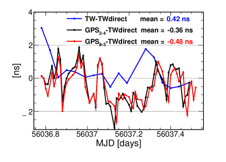
A dedicated two-way satellite link was used by US Naval Observatory (USNO) personnel to measure the time difference between ND and FD references using TWSTT. This involves exchanging signals between locations on a bi-directional satellite link, so that environmental and atmospheric effects are almost the same in each direction. The time difference calculated by double-differencing time-transfer between ND and FD with one GPS-based link and with the TWSTT link shows stability better than 800 ps and a mean difference (accuracy) of -480 ps. A secondary TWSTT mode was also employed using the USNO’s facility in Washington DC as a transfer point, and measuring FD-ND by the double-difference between USNO-ND and USNO-FD. No truly relativistic corrections are required in the TWSTT analysis apart from the formalism to correct for the rotation of the Earth (the Sagnac correction) Landau and Lifshitz (1962). Figure 3 shows the comparison between these time transfer techniques.
The same double difference computed between one GPS-based link and the TWSTT link can be performed between two GPS-based links, one using a pair of GPS receivers (one at each end of the link) and the other using the other pair. The comparison of the two GPS receivers at each location also allows the detection of eventual discrepancies between them. Since the calibration method simultaneously sets all GPS links between the two sites, the GPS-only double-differences constrain the calibration variation between calibrations. On the ND to FD link, the stability over the entire neutrino data collection period is better than 200 ps (). The mean difference of 205 ps, suggests a systematic uncertainty of 150 ps (half the error attributed to each link). We apply an overall systematic error of 500 ps due to the uncertainty in the overall FD-ND synchronization during the neutrino data collection period.
By using the two traveling GPS units it is possible to perform repeated calibrations of the stationary receivers at the various locations. Use of more than one calibration and the presence of a second receiver at each location allows the determination of possible time steps in any of the receiver’s internal time base. As an example, the double-difference between ND and FD, when calculated using the result of the same calibration over approximately eight months, showed a step of 2 ns. When the values of subsequent calibrations were considered, it became clear that the internal time base of one of the stationary receivers at the ND had a step of about the same magnitude. Two different calibration values were thus used for this receiver to remove the step from the double-difference, eliminating it from the error analysis for the synchronization.
IV Data Analysis
We select two categories of events whose selection criteria are described in Ref. Adamson et al. (2011): contained charged-current (CC) events, which originate in the fiducial region of each detector, and, for the FD only, partially reconstructed events. Partially reconstructed events are either CC neutrino interactions in the rock surrounding the FD producing an entering muon, or events where the neutrino interaction point occurred outside the detectors’ fiducial region. Partially reconstructed events usually arrive later than contained events, as the neutrino produces a muon at an angle, resulting in a trigonometric increase to the muon path-length (the muons are highly relativistic and their slightly slower-than-light speed does not contribute significantly to the later arrival). Both samples are subject to a further track-fit quality cut to ensure that we only use events with a well-measured interaction time. During March and April 2012, an exposure of protons on target was collected, yielding 195 fully contained and 177 partially reconstructed events which are selected at the FD.
The data analysis proceeds by using the measured time distribution of the protons in the RWCM to form a likelihood distribution for the time-of-flight of each neutrino event to each detector. A likelihood distribution is required because, for a given neutrino, we do not know which part of the accelerator spill (as shown in Fig. 1) is responsible for producing the observed neutrino. The RWCM timing waveform is convolved with a 1.5 ns (RMS) wide Gaussian distribution representing the detector timing resolution and shifted by the predicted time-of-flight to form a probability distribution function for the contained events. For partially reconstructed events, the probability density function is further convolved with a delay distribution to take account of the increased muon path length calculated using Monte Carlo simulations.
We multiply the event likelihoods of all the observed events together to obtain an overall probability as a function of the time-of-flight parameter. The time-of-flight which gives the maximum combined probability is then our measurement of the overall neutrino flight time from the RWCM to the detector. This procedure is followed at each of the two detectors.
To obtain the final result for the ND to FD time-of-flight, the two times obtained are subtracted, eliminating any systematic offset associated with the beam measurement and the portable detector measurement. Having two neutrino detectors, near and far, is unique to this measurement, as other neutrino time-of-flight analyses must rely on beam measurements.
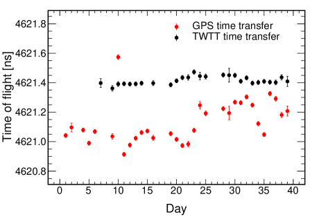
At the ND, the neutrino interaction rate is sufficient to measure the time-of-flight for each day with statistical error below 50 ps, permitting a test of the long-term stability of both the GPS and the TWTT timing systems using neutrinos directly, over the short baseline between RWCM and ND. The results from both these methods are shown in Fig. 4. The surveyed distance between the RWCM and the ND is combined with the absolute latency of the ND measured with the portable detector to create an expected time-of-flight of ns, where the uncertainty comes from the absolute latency of the portable detector and the RWCM-ND synchronization. Also included is a small effect of from the protons and pions traveling slightly below the speed of light and away from the beam axis.
| Systematic Uncertainty | Value |
|---|---|
| Inertial survey of the FD location | 2.3 ns |
| Relative ND-FD latency | ns |
| FD TWTT between surface and underground | 0.6 ns |
| GPS time-transfer accuracy | 0.5 ns |
Figure 4 shows that the daily measurements from both methods are contained within a 1 ns range consistent with this expectation. Note that the precision of this test is not as good as on the final time-of-flight result which benefits from the cancellation of uncertainty in the subtraction technique. Figure 4 shows that the time-of-flight measurements are stable to about 200 ps when using the GPS for time-transfer and to better than 50 ps when using the TWTT for time transfer. As the GPS time was common to both detectors and crosschecked by the USNO TWSTT measurement, the mean GPS-based value of 4621.1 ns is used later in calculating the final time-of-flight, with the difference being covered by the systematic error described in Sec.III.3.
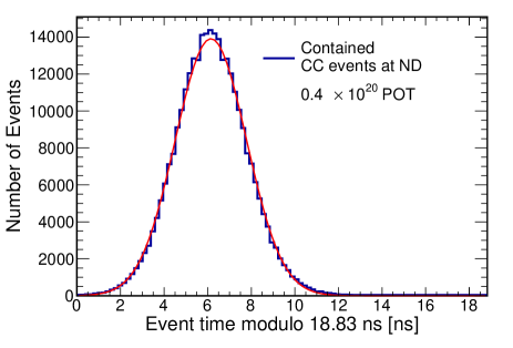
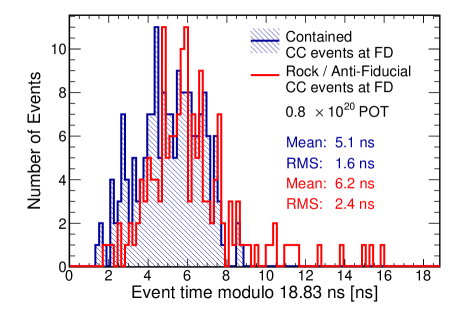
Figure 5 shows the neutrino arrival time distribution at the ND after the end of the preceding 18.83 ns long bunch, and Fig. 6 the same at the FD. The high neutrino statistics available at the ND illustrate that the neutrino production in a bunch is well fit by a Gaussian with a 1.6 ns sigma: this width is driven by the per-event 1.5 ns detector time resolution rather than the bunch width itself. The contained event sample at the FD is consistent with that distribution, confirming the resolution and stability of the time measurement system. The partially reconstructed events at the FD are also shown in Fig. 6 and are seen to arrive later and with a bigger spread as expected.
Combining the contained and partially reconstructed samples, the time-of-flight between the RWCM and FD is found to be ns, considering only statistical errors. Subtracting the measured time-of-flight (using GPS) between RWCM and ND of 4621.1 ns we obtain the time-of-flight between ND and FD as ns (statistical error only): the most precise measurement of the neutrino time-of-flight ever achieved, and the only one obtained directly using two neutrino detectors. The time required to traverse the distance between the front face of the Near and Far detectors at the speed of light, including the Sagnac correction, is ns, where the dominant uncertainty comes from the inertial survey of the FD location. Combining these, together with the other sources of systematic error listed in Table 1, yields a value for the difference in arrival time of the neutrino and the speed of light prediction of ns. The fractional neutrino speed is therefore found to be , consistent to 1 with relativistic neutrinos.
Acknowledgments
This work was supported by the U.S. DOE; the United Kingdom STFC; the U.S. NSF; the State and University of Minnesota; Brazil’s FAPESP, CNPq and CAPES. We are grateful to the Minnesota Department of Natural Resources and the personnel of the Soudan Laboratory, Fermilab, and USNO. We thank Texas Advanced Computing Center at The University of Texas at Austin for the provision of computing resources. Fermilab is Operated by Fermi Research Alliance, LLC under Contract No. De-AC02-07CH11359 with the United States Department of Energy.
References
- Hirata et al. (1987) K. Hirata et al. (KAMIOKANDE-II), Phys. Rev. Lett. 58, 1490 (1987).
- Bionta et al. (1987) R. Bionta et al. (IMB), Phys. Rev. Lett. 58, 1494 (1987).
- Alekseev et al. (1987) E. Alekseev et al. (Baksan), JETP Lett. 45, 589 (1987).
- Kalbfleisch et al. (1979) G.R. Kalbfleisch, N. Baggett, E.C. Fowler, and J. Alspector, Phys. Rev. Lett. 43, 1361 (1979).
- Adamson et al. (2007a) P. Adamson et al. (MINOS), Phys. Rev. D76, 072005 (2007a).
- Adam et al. (2011) T. Adam et al. (OPERA) (2011), eprint 1109.4897v2.
- Adam et al. (2012) T. Adam et al. (OPERA), JHEP 1210, 093 (2012), eprint 1109.4897v4.
- Antonello et al. (2012a) M. Antonello et al. (ICARUS), Phys. Lett. B713, 17 (2012a).
- Agafonova et al. (2012) N. Y. Agafonova et al. (LVD), Phys. Rev. Lett. 109, 070801 (2012).
- Antonello et al. (2012b) M. Antonello et al. (ICARUS), JHEP 1211, 049 (2012b).
- Adam et al. (2013) T. Adam et al. (OPERA), JHEP 1301, 153 (2013).
- Alvarez Sanchez et al. (2012) P. Alvarez Sanchez et al. (Borexino), Phys. Lett. B716, 401 (2012), eprint 1207.6860.
- Adamson et al. (2015) P. Adamson et al. (2015), eprint 1507.06690.
- Michael et al. (2008) D. G. Michael et al. (MINOS), Nucl. Instrum. Meth. A 596, 190 (2008).
- Adamson et al. (2013) P. Adamson et al. (MINOS Collaboration), Phys. Rev. Lett. 110, 251801 (2013).
- Blake (2005) A. Blake, Ph.D. Thesis, U. of Cambridge (2005).
- Adamson et al. (2007b) P. Adamson et al. (MINOS), Phys. Rev. D 75, 092003 (2007b).
- Cabrera et al. (2009) A. Cabrera et al. (MINOS), Nucl. Instrum. Meth. A609, 106 (2009).
- Cao (2014) S. Cao, Ph.D. Thesis, U. of Texas at Austin (2014).
- Crisp and Fellenz (2011) J. Crisp and B. Fellenz, JINST 6, T11001 (2011).
- (21) K. Seiya et. al. Proc. PAC09 (2009) p1424.
- Bocean (1999) V. Bocean (1999), prepared for 6th International Workshop on Accelerator Alignment (IWAA 99), Grenoble, France, 18-21 Oct 1999.
- Soler et al. (2000) T. Soler, R. H. Foote, D. Hoyle, and V. Bocean, Geophysical Research Letters 27, 3921 (2000).
- Skaloud and Schwarz (2000) J. Skaloud and K. Schwarz, Zeitschrift fuer Vermessungswesen (ZfV) (2000).
- Craymer et al. (2000) M. Craymer, R. Ferland, and R. Snay, in Towards an integrated global geodetic observing system (IGGOS) (Springer, 2000), pp. 118–121.
- Mortiz (1980) H. Mortiz, Bulletin Geodesique 54 (1980).
- (27) David W. Allan and Marc A. Weiss, Proc. 34th Ann. Freq. Control Symposium, USAERADCOM, Ft. Monmouth, NJ 07703, May 1980.
- (28) S. Römisch, et. al. Proc. 44th PTTI (2012) p99.
- (29) P. Adamson, et. al. Proc. 44th PTTI (2012) p119.
- Tètreault et al. (2005) P. Tètreault, J. Kouba, P. Hèroux, and P. Legree, Geomatica 59, 17 (2005).
- Webb and Zumberge (1995) F. Webb and J. Zumberge, Tech. Rep. JPL D-11088, Jet Propulsion Lab., Calif. Inst. of Technol., Pasadena (1995).
- Landau and Lifshitz (1962) L. D. Landau and E. M. Lifshitz, in Classical Theory of Fields (Pergamon Press, 1962), pp. 296–297.
- Adamson et al. (2011) P. Adamson et al. (MINOS), Phys. Rev. Lett. 106, 181801 (2011).