Universal spatial correlations in the anisotropic Kondo screening cloud: analytical insights and numerically exact results from a coherent state expansion

Abstract

We analyze the spatial correlation structure of the spin density of an electron gas in the vicinity of an antiferromagnetically-coupled Kondo impurity. Our analysis extends to the regime of spin-anisotropic couplings, where there are no quantitative results for spatial correlations in the literature. We use an original and numerically exact method, based on a systematic coherent-state expansion of the ground state of the underlying spin-boson Hamiltonian. It has not yet been applied to the computation of observables that are specific to the fermionic Kondo model. We also present an important technical improvement to the method, that obviates the need to discretize modes of the Fermi sea, and allows one to tackle the problem in the thermodynamic limit. As a result, one can obtain excellent spatial resolution over arbitrary length scales, for a relatively low computational cost, a feature that gives the method an advantage over popular techniques such as the Numerical and Density-Matrix Renormalization Groups. We find that the anisotropic Kondo model shows rich universal scaling behavior in the spatial structure of the entanglement cloud. First, SU(2) spin-symmetry is dynamically restored in a finite domain in parameter space in vicinity of the isotropic line, as expected from poor man’s scaling. More surprisingly, we are able to obtain in closed analytical form a set of different, yet universal, scaling curves for strong exchange asymmetry, which are parametrized by the longitudinal exchange coupling. Deep inside the cloud, i.e. for distances smaller than the Kondo length, the correlation between the electron spin density and the impurity spin oscillates between ferromagnetic and antiferromagnetic values at the scale of the Fermi wavelength, an effect that is drastically enhanced at strongly anisotropic couplings. Our results also provide further numerical checks and alternative analytical approximations for the Kondo overlaps that were recently computed by Lukyanov, Saleur, Jacobsen, and Vasseur [Phys. Rev. Lett. 114, 080601 (2015)] .

I Introduction

The spin $1/2$ Kondo model describes a localized magnetic moment interacting with an electron gas, via an antiferromagnetic exchange coupling.Hewson Despite a long history, and even an exact solution, it has not yet surrendered all its secrets. It is well established that the ground state is a spin singlet in which the impurity spin is quenched by the electron gas, and the spatial region where the electron gas is correlated with the impurity is referred to as the Kondo screening cloud.Affleck1 Even for an isotropic system, its precise spatial profile is not known analytically, except asymptotically,Affleck2 and it is only in the past few years that it has been calculated numerically.Gubernatis ; Borda ; Lechtenberg Despite wide-ranging proposals,Affleck3 ; Cornaglia ; Hand ; Pereira ; Park ; Nishida ; Bauer it has eluded direct measurement, partly because of the difficulty in measuring spin correlations.

In the isotropic case, the screening cloud is characterized by the ground state correlation function $X(x)=4\left<\vec{S}^{\rm imp}\cdot\vec{\mathcal{S}}^{\rm el}(x)\right>$ where $\vec{S}^{\rm imp}$ is the impurity spin operator, and $\vec{\mathcal{S}}^{\rm el}(x)$ is the electron spin density at $x$. When the Kondo temperature is much lower than the Fermi energy, the screening cloud can be decomposed into a forward scattering contribution $X_{0}(x)$ and a backscattering contribution $X_{2k_{F}}(x)$, so that $X(x)=X_{0}(x)+\cos(2k_{F}x)X_{2k_{F}}(x)$, where the two functions $X_{0}(x)$ and $X_{2k_{F}}(x)$ vary slowly on the scale of the Fermi wavelength $2\pi/k_{F}$. In the scaling regime and for spin-isotropic Kondo exchange, the profile of the screening cloud displays a universal line shape,Affleck4 ; Mitchell which is dependent on the value of Kondo coupling $J$ only through an emergent length $\xi$ that is inversely proportional to the Kondo temperature.Holzner ; Busser To be specific, if $X_{k}(x)$ and $X_{k}^{\prime}(x)$, with $k\in\{0,2k_{F}\}$, are correlation functions corresponding to different values $J$ and $J^{\prime}$ of the Kondo coupling, and $\xi$ and $\xi^{\prime}$ are the corresponding Kondo lengths, then

$$X_{k}^{\prime}(x)=\frac{\xi}{\xi^{\prime}}X_{k}(\xi^{\prime}x/\xi),$$ (1)

for all $x\gg 2\pi/k_{F}$.

Recently, we have realized that it may be possible to measure the longitudinal forward scattering ($k=0$) component of the screening cloud (a precise definition is given below) in a chain of tunnel-coupled superconducting islands.Snyman It turns out that the Hamiltonian describing the charge and phase degrees of freedom in this system is equivalent to the spin-anisotropic Kondo model in one dimension,Goldstein described by two coupling constants: The $z$-components of the impurity and electron spins couple with a strength $J_{\parallel}$, while the components perpendicular to the $z$-axis couple with a different strength $J_{\perp}$. A detailed study of the screening cloud in the anisotropic Kondo model has to our knowledge not been performed before, and is therefore timely.

In the anisotropic case, there are four correlation functions of interest, namely $X^{\parallel}_{k}(x)$, that measures the correlation between $z$-components of the impurity and electron spins (both in the forward $k=0k_{F}$ and backward $k=2k_{F}$ scattering channels), and $X^{\perp}_{k}(x)$, that measures correlations between components perpendicular to the $z$ axis (in each channel). Clearly, an anisotropic Kondo interaction, characterized by two coupling constants $J_{\parallel}$ and $J_{\perp}$, will affect the universal scaling picture non-trivially.

The universal scaling of the isotropic model has been confirmed using the Numerical Renormalization Group (NRG), a popular method to study the Kondo model.Borda ; Lechtenberg However, there is still room to improve the accuracy of existing results. For instance, it is predicted analytically Affleck1 that backscattering dominates forward scattering inside the screening cloud. This produces oscillations from ferromagnetic to antiferromagnetic correlations between the impurity and the electron gas, on the scale of half the Fermi wavelength. The first numerical calculation of the universal scaling functions were reported in Ref. Borda, . However, the predominance of the backscattering component over the forward scattering component inside the cloud was not resolved. This was probably due to the fact that results were obtained at relatively large Kondo temperatures, so that there was not a sufficient separation of scales between the size $\xi$ of the cloud, and the short distance ultraviolet cut-off scale. In a more recent work,Lechtenberg the NRG method of Ref. Borda, was refined, and the alternation of ferro- and antiferromagnetic correlations inside the cloud clearly be seen. However, results were only presented for distances up to $10$ Fermi wavelengths from the impurity. At these scales, the correlation functions show non-universal modulations.

In this Article, we perform numerical calculations that are sufficiently accurate to investigate the universal scaling behavior in regimes ranging from isotropic to strongly anisotropic Kondo couplings. At the same time, we can clearly resolve the predominace of the backscattering component over the forward scattering component inside the cloud. In precise terms, we investigate the the following questions: Let $X^{j}_{k}(x)$ and $(X^{j}_{k})^{\prime}(x)$, with $j\in\{\parallel,\perp\}$ and $k\in\{0,2k_{F}\}$, be correlation functions at distinct values $(J_{\perp},J_{\parallel})$ and $(J_{\perp}^{\prime},J_{\parallel}^{\prime})$. Under which conditions are there constants $\lambda_{1}$ and $\lambda_{2}$ such that $(X_{k}^{j})^{\prime}(x)=\lambda_{1}X_{k}^{j}(\lambda_{2}x)$, for all $x\gg 2\pi/k_{F}$, and what are the line shapes of these universal scaling curves? Our general numerical findings show that scaling is typically obeyed for fixed values of $J_{\parallel}$. In other words, correlators at the same $J_{\parallel}$ but different $J_{\perp}$ can be scaled onto each other. This statement holds as long as $J_{\perp}\lesssim 1$ (in dimensionless units of the inverse density of states), while for transverse couplings of order one, the Kondo temperature becomes comparable to the Fermi energy, and universality is lost. For $J_{\parallel}\gg J_{\perp}$, we find that the line shapes of the cloud correlation functions acquire a $J_{\parallel}$-dependence that cannot be scaled away. However, as $J_{\parallel}$ approaches $J_{\perp}$, the $J_{\parallel}$ dependence rapidly becomes very weak. One thus find a sizable region of parameter space, located around the strict spin-isotropic line $J_{\parallel}=J_{\perp}\lesssim 1$, in which the universal curves have little discernible $J_{\parallel}$ dependence. In this region, correlators calculated at $J_{\perp}\not=J_{\perp}^{\prime}$ and $J_{\parallel}\not=J_{\parallel}^{\prime}$ can to a very good approximation be scaled onto the unique universal curve of the isotropic model. These conclusions are consistent with poor man’s scaling arguments Chakravarty at small $J_{\perp}$, as we will explain in detail.

Our work also elaborates on a different but related topic, that was raised very recently by Lukyanov et al. in Ref. luk, , where the overlap between two Kondo wave functions with different Kondo couplings was computed analytically using integrability techniques, and numerically with the Density Matrix Renormalization Group. We complement these interesting results, by providing a simpler (approximate) analytical expression for the Kondo overlaps in the spin-anisotropic limit. We also show that our numerical method reproduces the full analytical result, as it should.

Regarding methodology, our approach combines both analytics and numerically exact calculations. In the case of strong spin-anisotropy, $J_{\parallel}\gg J_{\perp}$, we provide asymptotically exact formulas, that were not discussed in previous literature, for the fermionic Kondo cloud. For a general choice of parameters, we employ a recent approach using a coherent state expansion of the wave function, Bera1 ; Bera2 that has not yet been applied to the computation of purely fermionic observables that pertain to the Kondo model. This method relies on a variational Ansatz, formulated in the language of the spin-boson model, which describes a two-level system coupled to a multi-mode ohmic bosonic bath.Leggett ; Weiss This spin-boson model is known to be equivalent to the anisotropic Kondo model,Guinea with bosonization providing an exact mapping between the two.Kotliar ; Costi We exploit this mapping to apply the coherent-state expansion to the Kondo model. In addition, the flexible structure of the Ansatz allows one to add progressively more contributions to it, so that the method converges rapidly to the exact ground state with arbitrary accuracy.

Historically, the systematic coherent state expansion proposed by Bera et al. Bera1 ; Bera2 builds on seminal works of Emery and Luther,EmeryLuther and of Silbey and Harris,Silbey ; Harris in the language of the spin-boson model, and on independent works by Anderson,Anderson1 ; Anderson2 and Bergmann and ZhangBergmann in the language of the Kondo model. The approach of Emery and Luther, Silbey and Harris, and Anderson corresponds to the lowest order approximation, involving a single coherent state, and provides quantitatively accurate results only in the limit $J_{\parallel}\gg J_{\perp}$. Bergmann and Zhang took a step in the direction of a two coherent-state Ansatz by adding an extra term to the lowest order approximation, but constrained its form sub-optimally compared to the full solution with two coherent states. We stress that this type of approach differs from the well-known method pioneered by Yosida,Yosida1 that takes as starting point a state in which a single electron binds into a singlet with the impurity, while the rest of the Fermi sea is unaffected. The wave function of the bound electron is chosen to maximize the binding energy. The relationship between the Yosida approximation and the single-coherent state Ansatz is reminiscent of the relationship in superconductivity between the single Cooper pair on top of a Fermi sea on the one hand, and the full BCS wave function on the other. Yosida’s approach gives qualitatively correct results, but even when the effect of additional particle-hole excitations are included,Okiji ; Yosida2 it cannot yield arbitrarily accurate results for the correlations inside the Kondo screening cloud.

In this Article, we also contribute an important innovation to the coherent-state expansion methodology. In previous implementations, the bosonic bath was limited to a finite number of modes, because the number of variational parameters in the Ansatz scaled linearly with the number of bath modes. Here, we first partially solve the variational problem analytically, so that the number of remaining variational parameters that have to be determined numerically is independent of the number of bath oscillators. This allows us to take the thermodynamic limit before we optimize the energy numerically, and probe arbitrarily large distances. In the Kondo language, this means that we work directly with an infinite conductor.

With NRG, probing large length scales comes at the cost of losing information about shorter lengths scales. In order to maintain good spatial resolution, one has to introduce a fictitious impurity at the position where correlators are evaluated. Each position considered then requires the solution of a given two-channel Kondo impurity problem, so that a high-resolution computation of the Kondo cloud with NRG is quite expensive numerically. Our method remarkably deals with all length scales on an equal footing, so that the Kondo cloud can be calculated in a single step, once the many-body ground state is known. The coherent state expansion thus nicely complements the existing tools for studying the Kondo model.

The rest of the Article is structured as follows. In Sec. II we define the anisotropic Kondo Hamiltonian. We also state the equivalent spin-boson model, and the relation between the parameters of the two models. The precise mapping between them is reviewed in Appendix A. In Sec. III we define the spatial correlation functions, that contain information on the entanglement cloud around the spin impurity, and that we will study. We first consider the correlations in the fermionic language of the Kondo model and then in the bosonic language of the spin-boson model. The bosonic observables are derived from the fermionic ones in Appendix B. Sec. IV introduces the systematic coherent state expansion. The innovation we mentioned in the previous paragraph, that reduces the number of variational parameters to solve for numerically, is presented in Sec. V. In Sec. VI we take the thermodynamic limit for the energy, and express it in terms of the remaining variational parameters. The correlation functions that we study are expressed in terms of the remaining variational parameters in Sec. VII. Next, we find the optimal values for the variational parameters by minimizing the energy, and we present our results in Sec. VIII. We first confirm the accuracy of the method and then study in great detail the various correlation functions describing the Kondo cloud, as well as the Kondo wavefunction overlaps. Finally, in Sec. IX we summarize our main findings and, where applicable, compare them to results in the literature.

II Kondo and spin-boson Hamiltonians

In this section we write down the two related models that we study, and make explicit the deep connection between them. The first Hamiltonian is the anisotropic spin-$1/2$ Kondo model in one dimension, that describes a spin-1/2 impurity coupled to a Fermi sea. The Fermi sea does not necessarily represent electrons confined to one dimension. If the electron gas is higher dimensional, but the impurity is a point-like scatterer, it only interacts with electronic $s$-waves. Such $s$-waves in the electron gas can then be described by a one-dimensional Kondo Hamiltonian, where the spatial coordinate is the radial distance from the impurity. The second Hamiltonian is the ohmic spin-boson model, that appears in many area of physics, from superconducting nano-circuits to biological systems. Below an ultraviolet energy scale set by the Fermi energy, the two models are equivalent.Guinea ; Kotliar ; Costi The full mapping is reviewed in Appendix A.

The anisotropic spin-$1/2$ Kondo model in one dimension reads $H=H_{0}+H_{\parallel}+H_{\perp}$, where:

$$H_{0} = \sum_{k\sigma}(\varepsilon_{k}-\mu)\tilde{c}^{\dagger}_{k\sigma}\tilde{c}_{k\sigma},$$

$$H_{\parallel} = \frac{J_{\parallel}^{B}}{4}\sigma_{z}\left[\tilde{\psi}_{\uparrow}^{\dagger}(0)\tilde{\psi}_{\uparrow}(0)-\tilde{\psi}_{\downarrow}^{\dagger}(0)\tilde{\psi}_{\downarrow}(0)\right],$$

$$H_{\perp} = \frac{J_{\perp}^{B}}{2}\left[\tilde{\psi}^{\dagger}_{\uparrow}(0)\tilde{\psi}_{\downarrow}(0)\sigma^{-}+\tilde{\psi}^{\dagger}_{\downarrow}(0)\tilde{\psi}_{\uparrow}(0)\sigma^{+}\right].$$ (2)

Here $\tilde{c}_{k\sigma}$ annihilates an electron of wave number $k$ and spin direction $\sigma$ on a ring of length $L$, and $\tilde{\psi}_{\sigma}(x)=\sum_{k}e^{ikx}\tilde{c}_{k\sigma}/\sqrt{L}$. We denote these operators with tildes, because we will denote the useful slow modes (defined below) without tildes. We assume $\varepsilon_{k}=\varepsilon_{-k}$, so that there are both left and right-movers at the Fermi energy. The superscript $B$ indicates the bare values of the coupling constants $J^{B}_{\parallel}$ and $J^{B}_{\perp}$.

Integrating out high energy degrees of freedom towards the Fermi surface, we end up with a linear dispersion relation, and an effective low energy Hamiltonian:

$$H_{0} = \sum_{k\sigma}k\left(c^{\dagger}_{k\sigma}c_{k\sigma}+\bar{c}_{k\sigma}^{\dagger}\bar{c}_{k\sigma}\right),$$

$$H_{\parallel} = \frac{J_{\parallel}}{2}\sigma_{z}\left[\psi_{\uparrow}^{\dagger}(0)\psi_{\uparrow}(0)-\psi_{\downarrow}^{\dagger}(0)\psi_{\downarrow}(0)\right],$$

$$H_{\perp} = J_{\perp}\left[\psi^{\dagger}_{\uparrow}(0)\psi_{\downarrow}(0)\sigma^{-}+\psi^{\dagger}_{\downarrow}(0)\psi_{\uparrow}(0)\sigma^{+}\right],$$ (3)

in units where the Fermi velocity $v_{F}=1$. We have defined slow modes

$$c_{k\sigma} = \frac{1}{\sqrt{2}}\left(\tilde{c}_{k_{F}+k,\sigma}+\tilde{c}_{-k_{F}-k,\sigma}\right),$$

$$\bar{c}_{k\sigma} = \frac{1}{\sqrt{2}}\left(\tilde{c}_{k_{F}+k,\sigma}-\tilde{c}_{-k_{F}-k,\sigma}\right),$$

$$\psi_{\sigma}(x) = \frac{1}{\sqrt{L}}\sum_{k}e^{ikx}e^{-a|k|/2}c_{k\sigma},$$ (4)

and a similar relation between $\bar{\psi}_{\sigma}(x)$ and $\bar{c}_{k\sigma}$. Here $1/a$ is the ultraviolet cut-off energy. Operators without over-bars are associated with even-parity single particle wave functions, so that $c_{k\sigma}^{\dagger}$ creates an electron in the state $\sqrt{2/L}\cos[(k_{F}+k)x]$. In $D>1$ dimensions, an equivalent role is played by $s$-waves. For negative $x$, $\psi^{\dagger}_{\sigma}(x)$ creates an electron in an even-parity state consisting of two wave packets centered around $\pm x$ and propagating in opposite directions towards the impurity. For positive $x$ on the other hand, it creates an electron in a state consisting of two wave packets propagating away from the impurity. Because $\psi^{\dagger}_{\sigma}(x)$ and $\psi^{\dagger}_{\sigma}(-x)$ create electrons localized to the same physical regions in space, we refer to (3) as the unfolded representation. Operators with over-bars are associated with odd-parity single particle wave functions, so that $\bar{c}_{k\sigma}^{\dagger}$ creates an electron in the state $i\sqrt{2/L}\sin[(k_{F}+k)x]$. Since the even and odd modes decouple, and only the even modes couple to the impurity, we focus on electrons in even orbitals and drop the $\bar{c}^{\dagger}\bar{c}$ terms in $H_{0}$.

In the process of linearizing the spectrum (integrating out fast modes), the bare couplings $J^{B}_{\parallel}$ and $J^{B}_{\perp}$ are renormalized to new values $J_{\parallel}$ and $J_{\perp}$, that depend on the ultraviolet scale $1/a$. Note however that SU(2) symmetry, if present, is preserved under renormalization. Thus, if $J^{B}_{\perp}=J^{B}_{\parallel}$ (isotropic limit), then $J_{\perp}=J_{\parallel}$.

In this work, we will make extensive use of the well-known fact, reviewed in Appendix A, that the Kondo Hamiltonian (3) can be mapped onto an ohmic spin-boson model:

$$H_{\rm SB}=\sum_{q>0}qb_{q}^{\dagger}b_{q}-\sum_{q>0}\frac{g_{q}}{2}(b_{q}^{\dagger}+b_{q})s_{z}+\frac{\Delta}{2}s_{x}.$$ (5)

Here $b_{q}$ are bosonic operators such that $[b_{q},b_{q^{\prime}}]=0$ and $[b_{q},b_{q^{\prime}}^{\dagger}]=\delta_{q,q^{\prime}}$, while $s_{x}$ and $s_{z}$ are Pauli matrices. These pseudo-spin operators are not the physical angular momentum operators of the Kondo impurity, but are related to them. The parameters of the spin-boson model are related to those of the Kondo model by

$$g_{q}=2\sqrt{\frac{\alpha\pi q}{L}}e^{-aq/2},~{}\alpha=\left(1-\frac{J_{\parallel}}{2\pi}\right)^{2},~{}\Delta=\frac{J_{\perp}}{\pi a}.$$ (6)

III Screening cloud observables

Having defined the system we investigate, we now write down the observables that we will study. We are interested here in ground state correlation functions between the impurity spin and the electron spin density at a distance $x$ from the impurity, which we refer to collectively as the Kondo screening cloud (or cloud for short).Affleck1 We give equivalent expressions for the cloud correlators as ground state expectation values in both the fermionic and the bosonic pictures. In Appendix B the bosonic expressions are derived starting from the fermionic expressions.

In the fermionic picture, the cloud correlation functions is defined as:

$$X^{\parallel}(x)=4\left<S^{\rm imp}_{z}\mathcal{S}^{\rm el}_{z}(x)\right>_{\rm K},$$

$$X^{\perp}(x)=4\left<S^{\rm imp}_{x}\mathcal{S}^{\rm el}_{x}(x)+S^{\rm imp}_{y}\mathcal{S}^{\rm el}_{y}(x)\right>_{\rm K},$$ (7)

where $S_{j}^{\rm imp}=\sigma_{j}/2$ is the $j\in\{x,y,z\}$ component of the impurity spin operator, and

$$\mathcal{S}_{j}^{\rm el}(x)=\frac{1}{2}\sum_{\sigma\sigma^{\prime}}\tilde{\psi}_{\sigma}^{\dagger}(x)[\sigma_{j}]_{\sigma\sigma^{\prime}}\tilde{\psi}_{\sigma^{\prime}}(x)$$ (8)

is the $j$ component of the electron spin density at $x$. The subscript K indicates that the expectation value is with respect to the fermionic Kondo ground state. We refer to $X^{\parallel}$ as the longitudinal and $X^{\perp}$ as the transverse cloud. Both consist of a component $X^{j}_{0}$ that varies slowly on the scale of the Fermi wavelength, and a component that oscillates with wave vector $2k_{F}$, and has an amplitude $X^{j}_{2k_{F}}$ . The former is the result of scattering events that change the electron momentum by an amount that is small compared to $k_{F}$, while the latter results from scattering between the Fermi points at $\pm k_{F}$. Explicitly, one has:

$$X^{\perp}(x)=X^{\perp}_{0}(x)+\cos(2k_{F}x)X^{\perp}_{2k_{F}}(x),$$

$$X^{\parallel}(x)=X^{\parallel}_{0}(x)+\left[\cos(2k_{F}x)-\frac{a}{2x}\sin(2k_{F}x)\right]X^{\parallel}_{2k_{F}}(x).$$ (9)

For $x\gg a$, both the transverse and longitudinal $2k_{F}$ components are proportional to $\cos(2k_{F}x)$. In the bosonic language, and in the thermodynamic limit $|x|\ll L$, one finds using standard bosonization identities:

$$X^{\perp}_{0}(x)=\frac{a}{\pi(x^{2}+a^{2})}{\rm Re}\left<s^{-}e^{\varphi^{\dagger}(x)-i\varrho^{\dagger}(x)}e^{-\varphi(x)+i\varrho(x)}\right>+(x\to-x),$$

$$X^{\perp}_{2k_{F}}=\frac{2a}{\pi(x^{2}+a^{2})}{\rm Re}\left<s^{-}e^{\varphi^{\dagger}(x)}e^{-\varphi(x)}\right>,$$

$$X^{\parallel}_{0}(x)=\frac{\partial_{x}}{2\pi}\left<s_{z}\left[\varrho^{\dagger}(x)+\varrho(x)\right]\right>-\frac{a}{\pi(x^{2}+a^{2})},$$

$$X^{\parallel}_{2k_{F}}(x)=\frac{2x}{\pi(a^{2}+4x^{2})}{\rm Im}\left<s_{z}\left(\frac{a+ix}{a-ix}\right)^{s_{z}}e^{i\varrho^{\dagger}(x)}e^{i\varrho(x)}\right>,$$ (10)

with the bosonic fields:

$$\varphi(x)=2\sum_{q>0}\sqrt{\frac{\pi}{Lq}}e^{-aq/2}\left[\cos(qx)-1\right]b_{q},~{}~{}~{}\varrho(x)=2\sum_{q>0}\sqrt{\frac{\pi}{Lq}}e^{-aq/2}\sin(qx)b_{q}.$$ (11)

At $x<a$, the behavior of these expressions depend strongly on ultraviolet physics that our model does not attempt to represent accurately. The regime of physical significance is $x\gg a$ where the behavior of the cloud is insensitive to ultraviolet details of the model. None the less, we delay taking the $a/x\to 0$ limit until the end of the calculation, reasoning that it is of some interest to see how a particular cut-off scheme regularizes ultraviolet singularities.

We presented expressions for a one-dimensional cloud. However, the generalization to a higher dimensional electron gas is trivial, assuming a point impurity that therefore only scatters $s$-waves.Affleck1 In this case, one interprets the coordinate $x$ as a radial distance and divides the one-dimensional correlator by the area of a spherical shell of radius $x$. One also reverses the sign of the $2k_{F}$ components, because the radial part of the higher dimensional problem is defined on the half-line, with a $\pi$ phase shift between left- and right movers.

To make further progress in the computation of the cloud observables, we need an accurate approximation for the ground state of the spin-boson model. That is the topic of the next section.

IV Coherent-state expansion of the spin-boson ground state

We will use here a systematic coherent-state decomposition Bera1 ; Bera2 of the many-body ground state of the Ohmic spin-boson model. Physically, coherent states appear as natural degrees of freedom, because, in the absence of spin-tunneling $\Delta$, the two spin configurations are associated with a displacement of the bath modes from $0$ to $\pm f_{q}=\pm\sqrt{\pi\alpha/Lq}$. Indeed, at $\Delta=0$, there are two degenerate ground states

$$\left|f_{+}\right>\otimes\left|\uparrow\right>,~{}~{}~{}\left|f_{-}\right>\otimes\left|\downarrow\right>,$$ (12)

where

$$\left|f_{\pm}\right>=\exp\left[\pm\sum_{q>0}f_{q}(b_{q}^{\dagger}-b_{q})\right]\left|0\right>,$$ (13)

$\left|0\right>$ is the bosonic vacuum, and $\{\left|\uparrow\right>,\left|\uparrow\right>\}$ are the spin eigenstates of $s_{z}$. The single coherent-state Ansatz (usually dubbed the Silbey-Harris state) includes the effect of tunneling by promoting $f_{q}$ to a variational parameter and taking as trial state the linear combination $\left|f\right>=(\left|f_{+}\right>\otimes\left|\uparrow\right>-\left|f_{-}\right>\otimes\left|\downarrow\right>)/\sqrt{2}$. This results readily in the simple expression $f_{q}^{\mathrm{SH}}=\sqrt{\pi\alpha q/L}g_{q}/(q+\Delta_{R})$ with the self-consistency condition $\Delta_{R}=\Delta\left<f_{+}|f_{-}\right>=\Delta\left<f|-f\right>$. This trial wavefunction provides an excellent approximation to the true ground state provided the shifted equilibrium positions $f_{q}^{\mathrm{SH}}$ of most oscillators are not too far apart, i.e. if $\alpha$ is small compared to unity.

For larger $\alpha$, the overlap $\left<f\right|\left.-f\right>$, with $f_{q}$ determined variationally, becomes exponentially small, and this strongly underestimates the tunneling energy $\Delta\left<\sigma_{x}\right>/2$. The coherent-state expansion addresses this issue by extending the Silbey-Harris form to a more general linear superposition of coherent states:

$$\left|\psi\right>=\sum_{m=1}^{M}c_{m}\frac{\left|f^{(m)}\right>\otimes\left|\uparrow\right>-\left|-f^{(m)}\right>\otimes\left|\downarrow\right>}{\sqrt{2}},$$ (14)

with the set of displacement $f_{q}^{(m)}$ parametrizing a family of Silbey-Harris states:

$$\left|f^{(m)}\right>=\exp\left[\sum_{q>0}f^{(m)}_{q}(b_{q}^{\dagger}-b_{q})\right]\left|0\right>.$$ (15)

Here $M$ is the maximal number of allowed coherent states in the decomposition (14), and sets the level of approximation. The displacements $f^{(m)}_{q}$ and coefficients $c_{m}$ are determined by minimizing

$$\mathcal{E}=\left<\psi\right|H_{\rm SB}\left|\psi\right>-\lambda\left<\psi\right|\left.\psi\right>,$$ (16)

where $\lambda$ is a Lagrange multiplier that is used to enforce normalization. These parameters are generically found to be real in the ground state.

The coherent-state expansion already dramatically improves the estimate for the tunneling energy $\Delta\left<\psi\right|\sigma_{x}\left|\psi\right>/2$ for $M=2$, by allowing for cross-terms $\left<f^{(m)}\right|\sigma_{x}\left|f^{(n)}\right>$, in which the displacements $f_{q}^{(m)}$ and $f_{q}^{(n)}$ are anti-correlated at low $q$. Such cross-terms are therefore not exponentially small in $\alpha$, and allow a sizable energy gain compared to the Silbey-Harris approximation.

It is important to note that an arbitrary state of the spin-boson Hamiltonian can be written as an infinite but discrete sum of the form (14), at least if the bosonic bath contains a finite number of modes. This follows from a theorem, proved by Cahill,Cahill that for a single bosonic mode, countable sets $\left\{\left|f^{(m)}\right>,\,m=1,\,2,\,\ldots\right\}$ of (real) coherent states exist, that form a complete basis. For a finite number of bosonic modes, a general state can therefore be approximated to any required accuracy, by making $M$ sufficiently large. It is in this sense that the coherent state expansion is numerically exact, provided in practice that good convergence to the true many-body ground state occurs. Previous investigations Bera2 , as well as the extensive comparisons made in Sec. VIII, demonstrate indeed that the expansion (14) rapidly approaches the exact ground state of the spin-boson model as $M$ is increased to moderate values, also for an infinite bath.

V Reducing the number of variational parameters

In previous implementations of the coherent expansion (14-15), the bosonic bath was restricted to a large but finite number $N$ of modes, and each of the $M\times N$ displacements $f_{q}^{(m)}$ was treated as an independent variational parameter. In this work, we want to calculate the Kondo screening cloud, which requires a high spatial resolution from short to possibly exponentially large distances, so that a huge number of bath modes needs to be included. It is therefore desirable to have an implementation of the method in which the number of variational parameters does not depend on the number of included modes. Such an implementation would also allow for computations for a continuous spectral density (thermodynamic limit), which numerical techniques like NRG are not able to perform. In this section, we derive such an implementation, which is the the main technical innovation of our work.

We show that the algebraic structure of the variational equations constrains the functional dependence of the displacements $f^{(m)}_{q}$ with respect to momentum $q$ to such an extent that there are in fact only $M^{2}+M-1$ variational parameters, independently of the number of modes $N$ of the bosonic bath. To stress that the argument does not require a linear bath spectrum, we replace the term $\sum_{q>0}qb^{\dagger}_{q}b_{q}$ in the spin-boson Hamiltonian, with the more general kinetic energy expression $\sum_{q>0}\omega_{q}b_{q}^{\dagger}b_{q}$ for the remainder of this section. In subsequent sections, we will specialize again to the linear bath spectrum.

Exploiting the coherent state structure of the Ansatz, we can express the total energy $\mathcal{E}$ in terms of $f^{(m)}_{q}$ and $c_{m}$ as:

$$\mathcal{E}=\sum_{m,n=1}^{M}c_{m}c_{n}\left\{\left<f^{(m)}\right|\left.f^{(n)}\right>\sum_{q>0}\left[\omega_{q}f_{q}^{(m)}f_{q}^{(n)}-\frac{g_{q}}{2}\left(f_{q}^{(m)}+f_{q}^{(n)}\right)-\lambda\right]-\frac{\Delta}{2}\left<f^{(m)}\right|\left.-f^{(n)}\right>\right\},$$ (17)

where

$$\left<f^{(m)}\right|\left.\pm f^{(n)}\right>=\exp\left[-\frac{1}{2}\sum_{q>0}\left(f_{q}^{(m)}\mp f_{q}^{(n)}\right)^{2}\right].$$ (18)

Considering the minimization condition $\partial\mathcal{E}/\partial f_{q}^{(m)}=0$ with the use of (17) and (18), this leads to

$$\sum_{n=1}^{M}\left\{U_{mn}\omega_{q}+V_{mn}\right\}f_{q}^{(n)}=W_{m}g_{q},$$ (19)

where the entries of the $M\times M$ matrices $U$ and $V$, and the $M$-dimensional column vector $W$ are:

$$U_{lm}=2c_{m}\left<f^{(l)}\right|\left.f^{(m)}\right>,$$

$$V_{lm}=P_{lm}+Q_{lm}-\delta_{lm}\sum_{n}\left(P_{ln}-Q_{ln}\right),$$

$$P_{lm}=c_{m}\left<f^{(l)}\right|\left.f^{(m)}\right>$$

$$~{}~{}~{}~{}~{}~{}~{}~{}~{}~{}~{}~{}\times\sum_{k>0}\left[\omega_{k}f_{k}^{(l)}f_{k}^{(m)}-\frac{g_{k}}{2}\left(f^{(l)}_{q}-f^{(m)}_{q}\right)-\lambda\right],$$

$$Q_{lm}=c_{m}\frac{\Delta}{2}\left<f^{(l)}\right|\left.-f^{(m)}\right>,$$

$$W_{l}=\frac{1}{2}\sum_{m}U_{lm}.$$ (20)

It is crucial to note that $U$, $V$ and $W$ in (19) do not depend on the value of the momentum $q$ labelling the displacement $f_{q}^{(m)}$ that we consider within the variational equation. These matrices and vectors however depend non-linearly on the complete set of displacements, through summations over a dummy momentum index as in Eq. (18). From (19), it readily follows that $f_{q}^{(m)}$ is given by:

$$f_{q}^{(m)}=g_{q}\sum_{n=1}^{M}\left[(U\omega_{q}+V)^{-1}\right]_{mn}W_{n}.$$ (21)

Since $U\omega_{q}+V$ is linear in $\omega_{q}$,

$$\sum_{n=1}^{M}\left[(U\omega_{q}+V)^{-1}\right]_{mn}W_{n}=\frac{N^{(m)}(\omega_{q})}{D(\omega_{q})},$$ (22)

where $N^{(m)}(z)$ is a polynomial of order $M-1$ in $z$ and $D(z)={\rm det}(Uz+V)$ is a polynomial of order $M$ in $z$. Note that the denominator $D(z)$ is common to all sets of displacements $f^{(m)}$ for $m=1,\ldots,M$. Using the expression (20) for $W$ in terms of $U$, we see that for large $z$, $\frac{N^{(m)}(z)}{D(z)}\to 1/2z$ independent of $m$. Thus we arrive at the form:

$$f_{q}^{(m)}=\frac{g_{q}}{2}h_{m}(q),$$

$$h_{m}(q)=\frac{\sum_{n=0}^{M-1}\mu_{mn}\omega_{q}^{n}}{\prod_{n=1}^{M}(\omega_{q}-\omega_{n})},$$ (23)

where $\mu_{m\,M-1}=1$, and in general $\mu_{mn}$ is real. The poles $\omega_{n}$ that are not real come in complex conjugate pairs. The optimal state $\left|\psi\right>$ can be obtained by numerically minimizing the energy with respect to the $M\times(M-1)$ unknown coefficients $\mu_{mn}$, the $M$ poles $\omega_{n}$, and the $M-1$ weights $c_{m}$ (accounting for wavefunction normalization), so that there are $M^{2}+M-1$ parameters to be found in total, independently of the number of bosonic modes in the problem.

Since the dimension of the search space does not depend on the number of bath modes, the main obstacle in considering a bath with a very large number of modes has been removed. The next question is whether the energy, which involves sums over all bath modes, can be calculated efficiently for a large number of modes. Only single sums over the momentum have to be computed in the energy functional, and in the worst case, the total numerical cost is linear in the number of modes. This is a major improvement with respect to a brute force diagonalization of the model, where scaling of the Hilbert space dimension is exponential with the number of degrees of freedom. In order to reach the continuum limit, the discrete momentum sums are replaced by integrals, which fortunately can be performed analytically rather than numerically, as we now demonstrate.

VI Thermodynamic limit and the analytical evaluation of momentum integrals

In this section we specialize again to the case of a linear bath spectrum $\omega_{q}=q$, and analytically perform the momentum integrals involved in the calculating the energy for given set of variational parameters $\mu_{mn}$, $\omega_{m}$ and $c_{m}$. We do so for the smooth ultraviolet cut-off $g_{q}\propto e^{-aq/2}$ that the bosonization of the Kondo model naturally introduces. Although we do not work out the details here, we note that the momentum integrals can also be performed analytically in the case of a sharp cut-off $g_{q}\propto\theta(1/a-q)$. In the $L\to\infty$ (thermodynamic) limit, momentum sums are replaced by integrals according to

$$\frac{2\pi}{L}\sum_{q>0}\to\int_{0}^{\infty}dq.$$ (24)

With $f^{(m)}_{q}$ of the form (23), and $g_{q}$ of the form (6) dictated by the mapping from the Kondo model, the energy

$$E=\frac{\left<\psi\right|H_{\rm SB}\left|\psi\right>}{\left<\psi\right|\left.\psi\right>}$$ (25)

can be written as a functional of the variational parameters as:

$$E=\frac{\sum_{mn=1}^{M}c_{m}c_{n}\left(\alpha I_{mn}^{0}e^{-\frac{\alpha}{4}I^{-1}_{mn}}-\Delta e^{-\frac{\alpha}{4}I_{mn}^{+1}}\right)}{2\sum_{mn=1}^{M}c_{m}c_{n}e^{-\frac{\alpha}{4}I^{-1}_{mn}}},$$ (26)

which involves the Laplace transforms

$$I^{\lambda}_{mn}=\int_{0}^{\infty}dk\,e^{-ak}J^{\lambda}_{mn}(k)$$ (27)

of the rational functions

$$J_{mn}^{\pm 1}(k) = k\left[h_{m}(k)\pm h_{n}(k)\right]^{2},$$

$$J_{mn}^{0}(k) = \left[kh_{m}(k)-1\right]\left[kh_{n}(k)-1\right].$$ (28)

Note that we have omitted here a constant term

$$E_{0}=-\frac{\alpha}{2a},$$ (29)

that does not depend on the variational parameters. The functions $J_{mn}^{\lambda}(k)$ have $M$ second order poles of the type $(k-\omega_{l})^{-2}$. For large $k$, the behavior is

$$J_{mn}^{\lambda}(k)\simeq k^{-2+\lambda}.$$ (30)

The Laplace transforms can be performed analytically, using the following method. In general, we consider integrals of the form

$$I=\int_{0}^{\infty}dk\,e^{-ak}R(k),$$ (31)

where the function $R(k)$ is a ratio of polynomials, and all poles are of second order, i.e.

$$R(k)=\frac{p(k)}{\prod_{n=1}^{M}(k-\omega_{n})^{2}}.$$ (32)

This excludes the possibility of poles on the positive real line, which yields $E=+\infty$. Furthermore, the numerator $p(k)$ is a polynomial of at most order $2M-1$.

Figure 1: Chosen deformation of the contour for the integral (31).

It would be useful if we could replace the integration contour in (31) by a closed contour such as the one in Figure 1. We can do so, provided we multiply the integrand by a function $\mathcal{F}(k)$ with a branch cut along the positive real line such that $\mathcal{F}(k+i0^{+})-\mathcal{F}(k-i0^{+})\propto\theta(k)$. Furthermore, $\mathcal{F}$ must be such that the contribution to the integral that comes from closing the contour at large $k$ is negligible. A function that exactly meets these requirements is $\Gamma(0,-ak)$, where $\Gamma(0,z)$ is the incomplete Gamma function of order zero.nist It is defined as

$$\Gamma(0,z)=\int_{z}^{\infty}dt\,\frac{e^{-t}}{t},$$ (33)

where the integration path does not intersect the negative real line and excludes the origin. Its main relevant properties are

$$\Gamma(0,-(x+i0^{+}))-\Gamma(0,-(x-i0^{+}))=2\pi i,$$ (34)

for $x>0$, and

$$\Gamma(0,-z)\sim-\frac{e^{z}}{z},$$ (35)

for large $|z|$. Furthermore $\Gamma(0,-z)$ is analytical except in the neighborhood of the positive real line. Thus we find

$$\int_{0}^{\infty}dk\,e^{-ak}R(k)=\int_{C}\frac{dk}{2\pi i}\,R(k)e^{-ak}\Gamma(0,-ak)$$

$$=\sum_{n}{\rm Res}\left\{R(k)e^{-ak}\Gamma(0,-ak),\omega_{n}\right\}.$$ (36)

In the first line, $C$ is the contour depicted in Figure 1.

Returning to the integrals $I^{\lambda}_{mn}$ , one then has

$$I_{mn}^{\lambda}=\sum_{l=1}^{M}{\rm Res}\left\{J_{mn}^{\lambda}(k)e^{-ak}\Gamma(0,-ak),\omega_{l}\right\}.$$ (37)

Setting

$$F(z)=e^{-z}\Gamma(0,-z),$$ (38)

and noting that

$$\frac{d}{dz}F(z)=-\left[F(z)+\frac{1}{z}\right],$$ (39)

evaluation of the residues yield

$$I_{mn}^{\lambda}=\sum_{l}\dot{K}_{mnl}^{\lambda}F(\omega_{l}a)-K_{mnl}^{\lambda}\left(aF(\omega_{l}a)+\frac{1}{\omega_{l}}\right),$$ (40)

where

$$K_{mnl}^{\lambda} = \lim_{k\to\omega_{l}}(k-\omega_{l})^{2}J_{mn}^{\lambda}(k),$$

$$\dot{K}_{mnl}^{\lambda} = \lim_{k\to\omega_{l}}\frac{d}{dk}\left[(k-\omega_{l})^{2}J_{mn}^{\lambda}(k)\right].$$ (41)

To relate the $K$ parameters to the coherent state displacements explicitly, we define

$$h_{mn} = \lim_{k\to\omega_{n}}(k-\omega_{n})h_{m}(k)$$ (42)

$$= \frac{\sum_{l=0}^{M-1}\mu_{ml}\omega_{n}^{~{}l}}{\prod_{l=1\not=n}^{M}(\omega_{n}-\omega_{l})}$$

and

$$\dot{h}_{mn} = \lim_{k\to\omega_{n}}\frac{d}{dk}\left[(k-\omega_{n})h_{m}(k)\right]$$

$$= \frac{\sum_{l=1}^{M-1}l\mu_{ml}\omega_{n}^{~{}l-1}}{\prod_{l=1\not=n}^{M}(\omega_{n}-\omega_{l})}-h_{mn}\sum_{l=1\not=n}\frac{1}{\omega_{n}-\omega_{l}}.$$

This gives

$$K_{mnl}^{\pm 1} = \omega_{l}(h_{ml}\pm h_{nl})^{2},$$

$$K_{mnl}^{0} = \omega_{l}^{2}h_{ml}h_{nl},$$

$$\dot{K}^{\pm 1}_{mnl} = (h_{ml}\pm h_{nl})^{2}+2\omega_{l}(h_{ml}\pm h_{nl})(\dot{h}_{ml}\pm\dot{h}_{nl}),$$

$$\dot{K}^{0}_{mnl} = \omega_{l}(h_{ml}+\omega_{l}\dot{h}_{ml}-1)h_{nl}$$ (44)

$$~{}~{}+\omega_{l}h_{ml}(h_{nl}+\omega_{l}\dot{h}_{nl}-1).$$

Substitution of (44) into (40), and (40) into (26) yields an explicit expression for the energy in terms of the variational parameters.

As a consistency check, we can work out the single coherent state theory ($M=1$) to make sure that we recover the results of Silbey and Harris. This approximation is accurate for $\alpha\ll 1$, which, in the Kondo language, corresponds to the strongly anisotropic $J_{\parallel}\gg J_{\perp}$ regime. For $M=1$, there is only one variational parameter, which is conventionally defined as $\Delta_{R}=-\omega_{1}$. This translates to $h_{11}=1$ and $\dot{h}_{11}=0$ [see Eqs. (42) and (LABEL:defhd)]. The energy of the Silbey-Harris state then reads

$$E=-\frac{1}{2}\left[\alpha\Delta_{R}^{2}\partial_{\Delta_{R}}F(-\Delta_{R}a)+\Delta\left<f\right|\left.-f\right>\right],$$ (45)

with

$$\left<f\right|\left.-f\right>=\exp\left\{-\alpha\left[F(-\Delta_{R}a)+\Delta_{R}\partial_{\Delta_{R}}F(-\Delta_{R}a)\right]\right\},$$ (46)

and we have used the identity (39) to relate $F$ and its derivative. Minimizing $E$ with respect to $\Delta_{R}$, we recover the known self-consistency condition

$$\Delta_{R}=\Delta\left<f\right|\left.-f\right>.$$ (47)

Assuming than $\Delta_{R}\ll 1/a$, and using the fact that for small $z$,

$$F(-z)=-{\rm ln}(z)-\gamma_{E}+\mathcal{O}(z),$$ (48)

where $\gamma_{E}=0.577$ is the Euler-Mascheroni constant, one can solve the self-consistency condition for $\Delta_{R}$ to obtain

$$\Delta_{R}=\Delta\left(e^{1+\gamma_{E}}a\Delta\right)^{\frac{\alpha}{1-\alpha}}.$$ (49)

Up to a pre-factor, $\Delta_{R}$ corresponds to the Kondo temperature in the regime of small $\alpha$, where the single coherent state Ansatz is accurate.

In general, it is far more efficient to evaluate the energy analytically, as was done in this section, than to do the integrals in (26) numerically. There are however small regions of the search space where the analytical evaluation of the energy is not stable. These are regions in which two or more of the poles $\omega_{m}$ lie close to each other. In these regions, there are large cancellations between individual terms in the sum over residues in (37), and this leads to large numerical errors when individual residues are calculated separately before they are summed. We circumvent the problem as follows. When the minimization algorithm searches a dangerous region of the search space, it does not try to evaluate the residues at the offending poles individually. It rather takes the slow but safe option of numerically integrating around a loop that circles all closely spaced poles at a safe distance. Fortunately, one does not have to fall back on this contingency plan too often, as the problematic regions of the search space are small and do not seem to be particularly favored in the actual optimal solution.

VII Expressing the cloud with coherent states

In the previous section, we obtained an analytical expression for the energy in terms of $M^{2}+M-1$ variational parameters. This result allows for a significant speed-up of the numerical minimization of the energy. In this section, we apply the same analytical technique to evaluate the momentum integrals involved in the calculation of the Kondo screening cloud, in terms of bosonic displacements. Evaluating the four different cloud correlators (10) for the $M$-coherent state wavefunction can be done using straight-forward coherent-state algebra:

$$X_{0}^{\perp}(x) =-\frac{a}{\pi(x^{2}+a^{2})}\sum_{m,n=1}^{M}e^{\sqrt{\alpha}\left[A(0)_{mn}-A(x)_{mn}\right]}\cos(\sqrt{\alpha}B(x)_{mn})c_{m}c_{n}\left<f_{m}\right|\left.-f_{n}\right>,$$

$$X_{2k_{F}}^{\perp}(x) =-\frac{a}{\pi(x^{2}+a^{2})}\sum_{m,n=1}^{M}e^{\sqrt{\alpha}[A(0)_{mn}-A(x)_{mn}]}c_{m}c_{n}\left<f_{m}\right|\left.-f_{n}\right>,$$

$$X^{\parallel}_{0}(x) =-(1-\sqrt{\alpha})\frac{a}{\pi(x^{2}+a^{2})}+\frac{\sqrt{\alpha}}{2\pi}\sum_{m,n=1}^{M}C(x)_{mn}c_{m}c_{n}\left<f_{m}\right|\left.f_{n}\right>,$$

$$X^{\parallel}_{2k_{F}}(x) =\frac{2x}{\pi(4x^{2}+a^{2})}{\rm Im}\left[\frac{a+ix}{a-ix}\sum_{m,n=1}^{M}e^{i\sqrt{\alpha}D(x)_{mn}}c_{m}c_{n}\left<f_{m}\right|\left.f_{n}\right>\right],$$ (50)

together with the normalization condition

$$\sum_{m,n=1}^{M}c_{m}c_{n}\left<f_{m}\right|\left.f_{n}\right>=1.$$ (51)

The matrices $A$, $B$, $C$, and $D$ are defined as:

$$A(x)_{mn} =\int_{0}^{\infty}dq\,\cos(qx)e^{-aq}[h_{m}(q)+h_{n}(q)],$$

$$B(x)_{mn} =\int_{0}^{\infty}dq\,\sin(qx)e^{-aq}[h_{m}(q)-h_{n}(q)],$$

$$C(x)_{mn} =\int_{0}^{\infty}dq\,\cos(qx)e^{-aq}[qh_{m}(q)+qh_{n}(q)-2],$$

$$D(x)_{mn} =\int_{0}^{\infty}dq\,\sin(qx)e^{-aq}[h_{m}(q)+h_{n}(q)].$$ (52)

Note that $B$, $C$ and $D$ remain finite if the limit $a\to 0$ followed by $x\to 0$ is taken, while $A$ diverges logarithmically. The method we used to evaluate $\left<f_{m}\right|\left.\pm f_{n}\right>=\exp(-\alpha I_{mn}^{\mp 1}/4)$ analytically can be extended to evaluate the above integrals as well. The detail of the calculation can be found in Appendix C. The resulting expressions are:

$$A(x)_{mn} ={\rm Re}\sum_{l=1}^{M}(h_{ml}+h_{nl})F(\omega_{l}(a-ix)),$$

$$B(x)_{mn} ={\rm Im}\sum_{l=1}^{M}(h_{ml}-h_{nl})F(\omega_{l}(a-ix)),$$

$$C(x)_{mn} ={\rm Re}\sum_{l=1}^{M}\omega_{l}(h_{ml}+h_{nl})F(\omega_{l}(a-ix)),$$

$$D(x)_{mn} ={\rm Im}\sum_{l=1}^{M}(h_{ml}+h_{nl})F(\omega_{l}(a-ix)),$$ (53)

where $F(z)$ is defined in (38).

For future reference, we now consider the large (compared to the Kondo length) $x$ asymptotic behavior of the expressions (50) for the screening cloud. At $|z|\gg 1$,

$$F(z)\simeq\frac{-1}{z}-\frac{1}{z^{2}}.$$ (54)

The residue theorem can be used to derive the identities

$$\sum_{l=1}^{M}h_{ml}=1,~{}~{}~{}~{}\sum_{l=1}^{M}\frac{h_{ml}}{\omega_{l}}=-h_{m}(0).$$ (55)

With the aid of the above equations, the cloud correlators (50) are found to decay like $1/x^{2}$ at large $x$. Explicitly, one finds for $x\gg\xi_{\parallel}$:

$$X_{2k_{F}}^{\perp}(x)=X_{0}^{\perp}(x)=-\frac{2\xi_{\perp}}{x^{2}},$$

$$X_{2k_{F}}^{\parallel}(x)=X_{0}^{\parallel}(x)+\frac{a}{\pi x^{2}}=-\frac{\xi_{\parallel}}{x^{2}}$$ (56)

where the lengths $\xi_{\perp}$ and $\xi_{\parallel}$ are given by

$$\xi_{\perp}=\frac{a}{2\pi}\sum_{m,n=1}^{M}e^{\sqrt{\alpha}\sum_{l=1}^{M}(h_{ml}+h_{nl})F_{l}(a)}c_{m}c_{n}\left<f_{m}\right|\left.-f_{n}\right>,$$

$$\xi_{\parallel}=\frac{\sqrt{\alpha}}{2\pi}\sum_{m,n=1}^{M}[h_{m}(0)+h_{n}(0)]c_{m}c_{n}\left<f_{m}\right|\left.f_{n}\right>.$$ (57)

The above expression establishes a very direct connection between the $q=0$ behavior of the coherent state displacements and the large $x$ behavior of the longitudinal cloud. The small contribution $\mathcal{O}(a/x^{2})$ to $X^{\parallel}_{0}$ is a feature of the smooth ultraviolet cut-off $\sim e^{-aq}$, and will be ignored in what follows. Note that the $0k_{F}$ and $2k_{F}$ components of the cloud become equal at large $x$. Furthermore, there are two emergent length scales $\xi_{\perp}$ and $\xi_{\parallel}$ in the problem, which are in general not equal, unless spin-isotropy is restored.

In the single coherent-state approximation, which is accurate for small $\alpha$, the cloud correlators can be explicitly computed:

$$X_{0}^{\perp}(x)=X_{2k_{F}}^{\perp}(x)=-\frac{a\Delta_{R}}{\pi\Delta(x^{2}+a^{2})}e^{2\sqrt{\alpha}\left[F(-\Delta_{R}a)-{\rm Re}\,F(-\Delta_{R}(a-ix))\right]},$$

$$X_{0}^{\parallel}(x)=-(1-\sqrt{\alpha})\frac{a}{\pi(x^{2}+a^{2})}-\frac{\sqrt{\alpha}\Delta_{R}}{\pi}{\rm Re}\,F(-\Delta_{R}(a-ix)),$$

$$X_{2k_{F}}^{\parallel}(x)=\frac{2x}{\pi(a^{2}+4x^{2})}{\rm Im}\left[\frac{a+ix}{x-ix}e^{2i\sqrt{\alpha}{\rm Im}\,F(-\Delta_{R}(a-ix))}\right].$$ (58)

where, as noted in Sec. VI, $\Delta_{R}=-\omega_{1}$ is the Kondo energy scale. The two correlation lengths $\xi_{\perp}$ and $\xi_{\parallel}$ [cf. (57)] are in this anisotropic limit:

$$\xi_{\perp}=\frac{a\Delta_{R}}{2\pi\Delta}e^{2\sqrt{\alpha}F(-\Delta_{R}a)},~{}~{}~{}\xi_{\parallel}=\frac{\sqrt{\alpha}}{\pi\Delta_{R}}.$$ (59)

These simple analytical expressions for the Kondo cloud, valid in the limit of strong spin-anisotropy, have not appeared in the literature before. We will analyze them further in the next section, along with numerical results obtained for larger $\alpha$ values from the systematic coherent state expansion.

VIII Results

In Sec. VI and Sec. VII, we have collected the tools to calculate the average energy and the components of the screening cloud, for an $M$ coherent-state wavefunction, in terms of only $\mathcal{O}(M^{2})$ variational parameters. In order to find the variational parameters, the energy must be minimized, and for this purpose we use a standard simulated annealing algorithm.Corana ; Goffe Clearly, the quality of the approximation is limited by the maximum number of coherent states that can be handled with the available computational resources. Using a single personal computer and simulated annealing minimization, we have found it possible to go up to $M=7$ coherent states, which is enough for our purposes here, although an improved algorithm combining global and local optimization Bera2 can reach values as large as $M=24$. In fact, the required number of numerical operations is not a limitation per se here. Rather, the main difficulty is that the energy landscape in the space of variational parameters is very shallow and contains several low lying minima.

This section is divided into three extended sub-parts. First, we benchmark the coherent state method, both against previous results, and also by studying the convergence properties of the coherent state expansion, establishing its domain of validity for the computation of the screening cloud. Then, we consider the Kondo overlaps proposed in Ref. luk, , which we compute both analytically in the spin-anisotropic regime, and numerically for the nearly spin-isotropic case. Our results quantitatively agree with recent field theoretic calculations.luk We finally perform an extensive study of the Kondo cloud correlators over a wide range of parameter values by a combination of analytical arguments and extensive coherent state simulations. This allows us to uncover the precise universal features of the screening cloud of the anisotropic Kondo model.

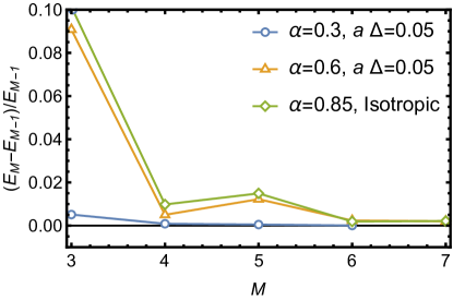
Figure 2: (color online) Fractional improvement $(E_{M}-E_{M-1})/E_{M-1}$ in the minimum energy $E_{M}$ as the number of coherent states $M$ is increased, at three different points in parameter space. Circles correspond to a strongly spin-anisotropic point $(\alpha=0.3,\Delta=0.05/a)$, triangles to a moderately spin-anisotropic point $(\alpha=0.6,\Delta=0.05/a)$, and diamonds to a perfectly spin-isotropic point $(\alpha=0.85,\Delta=0.156/a)$, associated to equal Kondo exchange couplings $J_{\perp}=J_{\parallel}=0.49$.

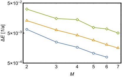
Figure 3: (color online) Energy uncertainty $\Delta E$ as a function of the number $M$ of coherent states, for the same three points in parameter space as the data in Figure 2.

VIII.1 Convergence properties of the coherent state expansion

In this subsection, we present strong evidence for the rapid convergence of the wavefunction (14) as the number $M$ of coherent states increases, using various observable quantities. In Refs. Bera1, and Bera2, , convergence was established only for a spin-boson model containing a large but finite number of modes, and we demonstrate here that fast convergence also occurs for a continuous bath spectrum.

We start by plotting in Figure 2 the fractional improvement $(E_{M}-E_{M-1})/E_{M-1}$ in the minimum energy $E_{M}$ obtained by adding an extra coherent state in the Ansatz, as a function of $M$. Note that, as in Sec. VI, we do not include the constant $E_{0}=-\alpha/{2a}$ in the definition of $E_{M}$. This convention leads to a denominator in $(E_{M}-E_{M-1})/E_{M-1}$ that is closer to zero, and therefore to a more stringent measure of convergence. Figure 2 shows results for three points in parameter space. One of the points, $(\alpha=0.3,\Delta=0.05/a)$, corresponds to a strongly anisotropic situation where convergence is very rapid. Another curve $(\alpha=0.6,\Delta=0.05/a)$ corresponds to a less anisotropic situation, where the convergence is slower. The remaining point $(\alpha=0.85,\Delta=0.156/a)$ corresponds to the isotropic coupling $J_{\perp}=J_{\parallel}=0.49$, or a Kondo temperature $T_{K}=\exp(-\pi/J)/a\simeq 1.6\times 10^{-3}/a$. For $(\alpha=0.3,\Delta=0.05/a)$, the minimum energy changes by an amount comparable to the accuracy goal of the minimization module, by the time that $M$ reaches $6$. For the other two points in parameter space, the marginal change in the minimum energy is a fraction of a percent at $M=7$. All the results that we present below are at least as converged as these last two cases.

As a complementary test, we can also verify that the multiple coherent state $\left|\psi\right>$ converges to an eigenstate of $H$ as the number of coherent states increases. To do so, we calculate the energy uncertainty

$$\Delta E=\sqrt{\left<\psi\right|H^{2}\left|\psi\right>-\left<\psi\right|H\left|\psi\right>^{2}},$$ (60)

for the optimal coherent states Ansatz $\left|\psi\right>$, as a function of $M$. For this purpose, an expression for the overlap $\left<f^{(m)}\right|H^{2}\left|f^{(n)}\right>$ is needed. It turns out that the same integrals $I^{\lambda}_{mn}$ as in Sect. VI are involved. In terms of these integrals, the overlap is expressed analytically as:

$$\left<f^{(m)}\right|H^{2}\left|f^{(n)}\right>$$

$$=\left\{\left(\frac{\alpha}{2}\right)^{2}\left(I_{mn}^{0}-\frac{1}{a}\right)^{2}+\left(\frac{\Delta}{2}\right)^{2}-\frac{\alpha}{2}\partial_{a}I_{mn}^{0}\right\}e^{-\frac{\alpha}{4}I_{mn}^{-1}}$$

$$+\frac{\alpha\Delta}{8}e^{-\frac{\alpha}{4}I_{mn}^{+1}}\partial_{a}\left(I_{mn}^{+1}-I_{mn}^{-1}\right).$$ (61)

The rest of the calculation can then proceed with the technology developed in Sect. VI for evaluating the integrals $I_{mn}^{\lambda}$. Note that derivatives $\partial_{a}I_{mn}^{\lambda}$, refer to partial derivatives with respect to the explicit $a$ dependence of the integrals, and not to total derivatives involving the implicit $a$-dependence of the variational parameters. The energy uncertainty $\Delta E$ is showed in Figure 3, as a function of coherent state number $M$, for the same three points in parameter space for which we have investigated the energy convergence above. In all three cases the energy uncertainty decreases monotonically, and roughly as a power law $\propto M^{-1.7}$. The fact that the uncertainty clearly tends to zero as $M$ increases, shows that the trial wavefunction (14) converges to the true ground state as the number of coherent states is increased.

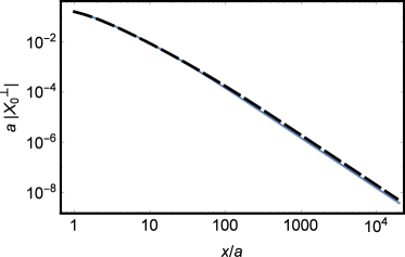
Figure 4: (color online) The $0k_{F}$ transverse component $X_{0}^{\perp}$ of the screening cloud, versus distance $x$ from the impurity, for $\alpha=0.1$, $\Delta=0.05/a$. The black dashed curve is the (fully converged) result of a $6$ coherent state calculation. The solid blue curve corresponds to the single coherent state result (58). In the spin-anisotropic limit $\alpha\ll 1$, the single coherent state approximation is thus very accurate.

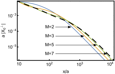
Figure 5: (color online) Convergence of the cloud for the $0k_{F}$ transverse component $X_{0}^{\perp}$ versus distance $x$, for $\alpha=0.85$, $\Delta=0.156/a$. This parameter choice corresponds to an isotropic Kondo coupling $J_{\perp}=J_{\parallel}=0.49$. The black dashed line represents the result of a $M=7$ coherent state calculation, while solid curves represent results for $M=2,\,3$ and $5$ coherent states.

Next, we investigate the convergence of the screening cloud itself. In Figure 4 we show an instance of very rapid convergence in the case of strong spin-anisotropy, and in Figure 5 an example where there is a noticeable change between $M=1$ and $M=7$ coherent states (note also that this data set is one of the least converged ones included in this work). In both figures we plot the $0k_{F}$ transverse correlator $X_{0}^{\perp}(x)$, as we found this component to show the most dramatic change as $M$ is increased. Figure 4 corresponds to $\alpha=0.1$ and $\Delta=0.05$ (strong spin-anisotropy), and the comparison to a $M=6$ coherent state calculation shows that the single coherent state (Silbey-Harris Ansatz) is nearly exact in this limit. The results in Figure 5 were obtained at $\alpha=0.85$ and $\Delta=0.156/a$, which corresponds to an isotropic Kondo coupling $J_{\perp}=J_{\parallel}=0.49$, for $M=2,\,3,\,5$ and $7$ coherent states. Good convergence is clearly ensured by the computation with $M=7$ coherent states.

VIII.2 Comparison to exact results based on integrability: ground state energy and Kondo overlaps

In this subsection, we give further evidence that ground state properties of the Kondo model can be calculated accurately using the coherent state expansion. In particular, we focus here on several physical quantities that can be computed exactly via the Bethe Ansatz or related integrability techniques.

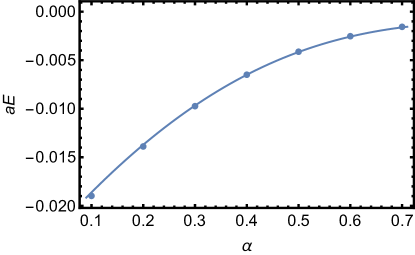
Figure 6: (color online) Ground state energy versus $\alpha$ as obtained via the multiple coherent state approximation (dots) and the exact Bethe Ansatz solution (solid line), for $\Delta=0.05/a$.

In Figure 6, we compare the multiple coherent state estimate for the ground state energy to results obtained via the exact Bethe Ansatz hur , at $\Delta=0.05/a$ and various $\alpha$ values. The high energy cutoff $1/a$ corresponds to the parameter $\omega_{c}$ in Ref. hur, , and we used from this reference expression (C.9) for the ground state energy and equation (8) for the Kondo temperature $T_{K}$, with the relationship between $D$ and $\omega_{c}$ given in (C.8). Although our calculation is variational, the energy is typically converged to about 0.1% (see Figure 2). One has to bear in mind however that, in the ultraviolet, the model for which the Bethe Ansatz yields the exact solution differs from the model we consider here. The Bethe Ansatz result is only valid if all relevant energy scales in the problem are much smaller than the ultraviolet cut-off scale. For finite $\Delta a$, the Bethe Ansatz expressions even present spurious divergences around $\alpha=(2n+1)/(2n+2)$, for $n=1,\,2,\,\ldots.$ As a result, exact agreement can only be expected at $|Ea|\ll 1$, and this explains why our variational result is slightly off the Bethe Ansatz result for small $\alpha$, although the variational approach presents better convergence in this regime. In general, the numerical data agrees so closely with the Bethe Ansatz result that it is impossible to distinguish between errors resulting from truncation of the coherent state expansion at $M=7$ and errors due to ultraviolet differences between the models.

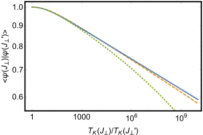
Figure 7: (color online) Kondo overlap $\left<\psi(J_{\perp})\right|\left.\psi(J_{\perp}^{\prime})\right>$ between ground states at different and varying values of $J_{\perp}$, but with the same fixed value of $J_{\parallel}$, versus the ratio $T_{K}(J_{\perp})/T_{K}(J_{\perp}^{\prime})$. Here, the strongly spin-anisotropic regime is considered with $\alpha=0.1$, i.e. $J_{\parallel}=4.30$. The solid line shows the single coherent state formula (65), whereas the dashed line is the exact analytical result (62). The dotted line is the small $\alpha$, small $|z|$ approximation (66).

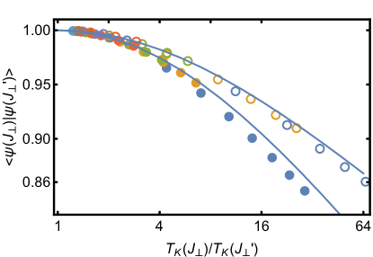
Figure 8: (color online) Kondo overlap $\left<\psi(J_{\perp})\right|\left.\psi(J_{\perp}^{\prime})\right>$ at intermediate $\alpha$ values. Open symbols in various colors show the $M=6$ coherent state results for $J_{\parallel}=0.905$ (i.e. $\alpha=0.3$) for several values of $J_{\perp}$ and $J_{\perp}^{\prime}\in[0.016,0.346]$ (i.e. $\Delta\in[0.005/a,0.110/a]$). Closed symbols show the $M=7$ coherent state results for $J_{\parallel}=0.451$ (i.e. $\alpha=0.6$) for several values of $J_{\perp}$ and $J_{\perp}^{\prime}\in[0.016,0.346]$ (i.e. $\Delta\in[0.236/a,0.785/a]$). Solid curves represent the exact analytical result (62). The Kondo temperature was taken from the approximate identification $T_{K}=1/\xi_{\parallel}$.

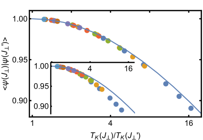
Figure 9: (color online) Kondo overlap $\left<\psi(J_{\perp})\right|\left.\psi(J_{\perp}^{\prime})\right>$ at $\alpha=0.8$ ($J_{\parallel}=0.663$). Open symbols in various colors show the $M=7$ coherent state results for several values of $J_{\perp}$ and $J_{\perp}^{\prime}\in[0.377,0.880]$ (i.e. $\Delta\in[0.12/a,0.28/a]$). Solid curves represent the exact analytical result (62). In the main panel, the improved renormalization group estimate (64) was used for $T_{K}$. In the inset, the less accurate value $T_{K}=1/\xi_{\parallel}$ was used.

Another interesting quantity for which an exact analytical result has recently been obtained luk , and which gives some indirect information on the Kondo cloud, is the overlap $\left<\psi(J_{\perp})\right|\left.\psi(J_{\perp}^{\prime})\right>$ of two Kondo ground states with different transverse exchange couplings, as a function of the Kondo temperature ratio $T_{K}(J_{\perp})/T_{K}(J_{\perp}^{\prime})$. Here $\left|\psi(J_{\perp})\right>$ and $\left|\psi(J_{\perp}^{\prime})\right>$ denote the full many-body ground states obtained at different $J_{\perp}$ but for the same $J_{\parallel}$, while $T_{K}(J_{\perp})$ and $T_{K}(J_{\perp}^{\prime})$ are the associated Kondo temperatures. With the definition $z={\rm ln}[T_{K}(J_{\perp}^{\prime})/T_{K}(J_{\perp})]$, the exact result reads:

$$\left<\psi(J_{\perp})\right|\left.\psi(J_{\perp}^{\prime})\right>=\frac{1}{1-\alpha}\frac{\sinh[(1-\alpha)z/2]}{\sinh(z/2)}g_{\alpha}(z),$$

$$g_{\alpha}(z)=\exp\left[\int_{0}^{\infty}\frac{dt}{t}\frac{\sin^{2}(zt/\pi)}{\sinh(2t)\cosh(t)}\frac{\sinh\left(\frac{\alpha t}{1-\alpha}\right)}{\sinh\left(\frac{t}{1-\alpha}\right)}\right].$$ (62)

When comparing our numerical results to this analytical formula, a subtle issue arises. The Kondo temperature is certainly related to the inverse of the size of the screening cloud, but the exact relation may well involve an $\mathcal{O}(1)$ factor that is $J_{\perp}$ dependent. We have therefore tried various definitions of the Kondo temperature. For small to moderate $\alpha$, we find that $T_{K}\propto 1/\xi_{\parallel}$, as defined in Eq. (56), with a $J_{\perp}$-independent proportionality constant, works well. Indeed, in the Silbey-Harris regime, this correspondence is exact (see below). For larger $\alpha$ however, this definition seems to incur a systematic error. For $J_{\parallel}$ and $J_{\perp}$ relatively small, as is exemplified by the data we collected at $\alpha=0.8$, we have found it better to estimate the Kondo scale from direct integration of the standard weak-coupling in $J_{\perp}$ and $J_{\parallel}$ poor man’s scaling equations:

$$\frac{dJ_{\perp}}{dl}=\frac{1}{\pi}J_{\parallel}J_{\perp},~{}~{}~{}\frac{dJ_{\parallel}}{dl}=\frac{1}{\pi}J_{\perp}^{2},$$ (63)

which lead to an expression of the Kondo scale for the spin-anisotropic Kondo model that is valid for $J_{\parallel}\ll 1$ and $J_{\perp}\ll 1$:

$$T_{K}=\frac{1}{a}\exp\left[-\frac{\pi}{\sqrt{J_{\perp}^{2}-J_{\parallel}^{2}}}\arctan\left(\frac{\sqrt{J_{\perp}^{2}-J_{\parallel}^{2}}}{J_{\parallel}}\right)\right].$$ (64)

Let us first consider the regime of small $\alpha$. Here we have seen that single coherent state results are already well-converged. In the single coherent state approximation, the overlap is given by:

$$\left<\psi(J_{\perp})\right|\left.\psi(J_{\perp}^{\prime})\right>=\exp\frac{\alpha}{2}\left[1-\frac{\bar{z}}{2}\coth(\bar{z}/2)\right],$$ (65)

where $\bar{z}=\ln\,[\Delta_{R}(J_{\perp}^{\prime})/\Delta_{R}(J_{\perp})]$. For small $\alpha$, Ref. luk, quotes the “semi-classical” result,

$$\left<\psi(J_{\perp})\right|\left.\psi(J_{\perp}^{\prime})\right>=1+\frac{\alpha}{2}\left[1-\frac{z}{2}\coth(z/2)\right],$$ (66)

which can be obtained by expanding the exact result (62) to first order in $\alpha$. Since $z\coth(z/2)$ grows linearly in $z$ for large $z$, the semi-classical result can at best only be valid for $z$ sufficiently smaller than $1/\alpha$. Referring back to the single coherent state result (59) for the correlation lengths, we see that if we make the identification $T_{K}\propto 1/\xi_{\parallel}$, the single coherent state approximation (65) is nothing but a resummation of the small $\alpha$ result in Ref. luk, , in which $\ln\left<\psi(J_{\perp})\right|\left.\psi(J_{\perp}^{\prime})\right>$ is calculated to second order in the impurity interaction, and then exponentiated. In Figure 7 we compare the single coherent state approximation to the exact result (62). we see that, unlike the semiclassical formula (66), the single coherent state approximation remains valid up to large ratios of the Kondo temperatures, because the ground state is well captured for any value of the Kondo temperature (provided $\alpha$ is small enough).

We now turn to the regime of larger dissipation, and in Figure 8 we show multiple coherent state results for the Kondo overlap at $\alpha=0.3$ and $\alpha=0.6$, again using the (now approximate) identification $T_{K}\propto 1/\xi_{\parallel}$, together with the exact result (62). Data points of the same color were obtained by keeping $J_{\perp}$ fixed and varying $J_{\perp}^{\prime}<J_{\perp}$. If two data points have different colors, they correspond to distinct $J_{\perp}$ and $J_{\perp}^{\prime}$. It is therefore already nontrivial that the differently colored points fall on the same curve, confirming the universality predicted by the exact analytical expression (62). Generally, good agreement with the analytical result (62) is seen, with only a small systematic error pushing the numerical curves slightly below the analytical ones, which increases as $\alpha$ increases. A small part of the error is likely due to an error of a few percent in the numerical estimation of $\xi_{\parallel}$, and to $T_{K}$ being only an order of magnitude or so less than the ultraviolet scale $1/a$ at large $J_{\perp}$. These errors would be reduced if we could use more coherent states and smaller $J_{\perp}$. However, as pointed out earlier, the main discrepancy comes from the chosen definition of the Kondo temperature in Ref. luk, , which is not exactly equivalent to $1/\xi_{\parallel}$ at larger $\alpha$. Indeed, Figure 9 shows the multiple coherent state results for the overlap at $\alpha=0.8$, using both the naive identification $T_{K}\propto 1/\xi_{\parallel}$ (inset) and the renormalization improved estimate (64). The latter choice leads clearly to a substantial reduction of the error. Our conclusion is that the actual Kondo overlap $\left<\psi(J_{\perp})\right|\left.\psi(J_{\perp}^{\prime})\right>$ is calculated quite accurately in the coherent state expansion, and that the (modest) observed errors are associated with the extraction procedure of the Kondo temperature from the size of the cloud.

VIII.3 Comparison to the exact longitudinal forward-component of the cloud at the Toulouse point

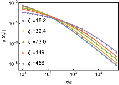
Figure 10: (color online) The longitudinal $0k_{F}$ component of the screening cloud at the Toulouse point $\alpha=1/2$. Five different values of $\Delta$ ranging from $0.02/a$ to $0.1/a$ were used. The symbols correspond to results obtained with the coherent state expansion (truncated at $M=7$ terms) for a choice of discrete positions, while the solid lines represent the exact result (67). Also indicated for each curve is the associated Kondo length $\xi_{\parallel}$, ranging from $18.2a$ at $\Delta=0.1/a$ to $456a$ at $\Delta=0.02/a$.

In this subsection provide strong evidence that the coherent state expansion (14) captures the full spatial structure of the Kondo cloud, using an exact analytical result at the so-called Toulouse point. Indeed, at $J_{\parallel}=2\pi(1-1/\sqrt{2})$ or equivalently, $\alpha=1/2$, the Kondo model is equivalent to a fermionic non-interacting resonant level model [Zarand, ]. An exact result for the longitudinal $0k_{F}$ component of the screening cloud can be obtained following the route set out in Refs. Posske1, and Posske2, . We review this calculation in Appendix D. The result is given by the simple formula

$$X_{0}^{\parallel}(x)=-\frac{\sqrt{2}}{\pi^{2}}\frac{J_{\perp}^{2}}{4\pi a}F\left(-\frac{J_{\perp}^{2}|x|}{4\pi a}\right)^{2},$$ (67)

with $F$ as defined in Eq. (38). From the point of view of the coherent state expansion, there is nothing special about the Toulouse point. In the coherent state expansion, $X_{0}^{\parallel}$ is expressed as a linear combination of $F$ functions with different position dependent arguments, cf. Eq. (53), and an infinite number of terms are required to approximate $F^{2}$ exactly. In Figure 10, we compare the exact expression to results obtained with the coherent state expansion, truncated at $M=7$ terms. For clarity, we show here results of the coherent state expansion only for a discrete set of $x$ values, because the complete curves would have completely covered the exact result. We clearly find near perfect agreement between the coherent state expansion and the exact result. Since the coherent state expansion does not exploit any special features of Toulouse point, we expect similar accuracy at a similar cost ($M=7$) to be achievable at other values of $\alpha$.

VIII.4 Detailed analysis of the screening cloud

Having thoroughly established the accuracy of the coherent state approximation for the Kondo ground state, we now proceed to investigate the physical features of the Kondo screening cloud, both for isotropic and anisotropic regimes.

VIII.4.1 Summary of known results

We first briefly recall the available analytical results regarding the isotropic screening cloud. In the isotropic case ($J_{\perp}=J_{\parallel}$), the transverse components of the screening cloud equal twice the longitudinal components, i.e.

$$X_{0}^{\parallel}=X_{0}^{\perp}/2\equiv X_{0},~{}~{}X_{2k_{F}}^{\parallel}=X_{2k_{F}}^{\perp}/2\equiv X_{2k_{F}}.$$ (68)

For $x\gg a$, both $X_{0}(x)$ and $X_{2k_{F}}(x)$ are expected to be universal scaling functions

$$\xi X_{k}(x)=\tilde{X}_{k}(\tilde{x}),~{}~{}\tilde{x}=x/\xi,~{}~{}k=0,\,2k_{F}.$$ (69)

Here $\tilde{X}_{k}$ is independent of $J$, and all parameter dependence is contained in the Kondo length $\xi$. The Kondo length is expected to be inversely proportional to the Kondo temperature, but the exact relation may contain a $J$-dependent proportionality factor of order unity, as we discussed previously. The following asymptotic results for $\tilde{X}_{0}$ and $\tilde{X}_{2kF}$ have been derived analytically Affleck1 :

$$\tilde{X}_{0}(\tilde{x})\propto-\frac{1}{\tilde{x}(\ln\tilde{x})^{2}},~{}~{}\tilde{X}_{2k_{F}}(\tilde{x})\propto\frac{1}{\tilde{x}\ln\tilde{x}},~{}~{}~{}\mathrm{for}~{}\tilde{x}\ll 1$$

$$\tilde{X}_{0}(\tilde{x})\simeq\tilde{X}_{2k_{F}}(\tilde{x})\simeq-\frac{1}{\tilde{x}^{2}}~{}~{}~{}\mathrm{for}~{}\tilde{x}\gg 1.$$ (70)

The regime of small $\tilde{x}$ is perturbatively accessible with a calculation using renormalization group techniques, while the large $\tilde{x}$ regime is treated using Fermi liquid theory. Note that at small $\tilde{x}$, the $2k_{F}$-oscillatory component of the cloud dominates the $0k_{F}$ component slightly. This implies that the total correlation function $X(x)=X_{0}(x)+\cos(2k_{F}x)X_{2kF}$ oscillates between positive and negative values, with wavelength $\pi/k_{F}$ at small $x$. In other words, close to the impurity, the spin correlations between the electron gas and the impurity alternate between being ferromagnetic and being antiferromagnetic, on the scale $\pi/k_{F}$. The crossover from slower than $1/\tilde{x}$ decay inside the cloud to $1/\tilde{x}^{2}$ decay at large $x$ is expected to occur at $x\sim\xi$, i.e. $\tilde{x}\sim 1$. Our goal in the next paragraph is to confirm these results for the isotropic cloud, and to compute the full crossover curve from the coherent state expansion. In a second step, we will examine how the cloud correlations change when the Kondo couplings are not isotropic ($J_{\perp}\not=J_{\parallel}$).

VIII.4.2 Kondo cloud in the isotropic case

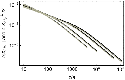
Figure 11: The four components of the isotropic screening cloud: the top panel represents the longitudinal (black) and transverse (gray) $0k_{F}$ components, while the bottom panel represents the longitudinal (black) and transverse (gray) $2k_{F}$ components. The calculation was performed for the choice of Kondo couplings $J=0.42,\,0.49,\,0.66,$ and $0.84$, which correspond to $\alpha=0.87,\,0.85,\,0.8,$ and $0.75$. The various curves can be identified from the fact that the crossover to faster $1/x^{2}$ decay occurs on an increasing length scale $\xi$ as $\alpha$ is increased (or equivalently $J$ is decreased). For $\alpha=0.75$ convergence was achieved with $M=5$ coherent states, while for the other values of $\alpha$, $M=7$ was required.

As a first step, we present results in Figure 11 for the screening cloud calculated for several parameters on the isotropic line $J_{\perp}=J_{\parallel}$, or equivalently $\alpha=(1-a\Delta/2)^{2}$. The correlation functions are plotted in units of $1/a$ on the vertical axis and in units of $a$ on the horizontal axis. When considering the small $\tilde{x}$ regime numerically, one must remember that $x$ has to remain sufficiently larger than the short distance ultraviolet cut-off $a$, since the limits $a\to 0$ and $x\to 0$ do not commute. This restriction is implied whenever we consider the asymptotic $\tilde{x}\to 0$ limit. The transverse and longitudinal components are plotted in the same panel, and we expect $X_{k}^{\parallel}=X_{k}^{\perp}/2$ for both the $k=0k_{F}$ and $k=2k_{F}$ components due to strict spin-isotropy. The numerical results of Figure 11 reveal this isotropy to a high degree, and this is a non-trivial check of our method, since rotational symmetry in the bosonic model is only emergent. It is violated by the ultraviolet regularization (see Appendix A). This fact also explains the small differences that are still visible between the transverse and longitudinal components.

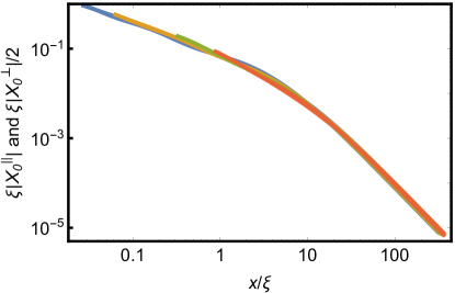
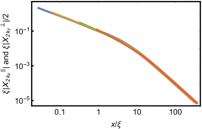
Figure 12: (color online) The isotropic correlation functions of Figure 11, in rescaled units $1/\xi$ on the vertical axis and $\xi$ on the horizontal axis. The Kondo length $\xi=\xi_{\parallel}$ was estimated from Eq. (57).

In Figure 12 we plot the same data as in Figure 11, but now in rescaled units, according to (69). We ignored small differences between the large distance behavior of the transverse and longitudinal components, and scaled all components with $\xi=\xi_{\parallel}$, where the Kondo length $\xi_{\parallel}$ was calculated using Eq. (57). We clearly see that it is possible to scale correlation functions calculated at different $J$ onto universal curves. As expected, we observe that the cross-over from slower than $1/x$ decay inside the cloud to $1/x^{2}$ decay at large $x$ occurs around $x\sim\xi$. The precise behavior of the Kondo length $\xi$ as a function of $J$ will be analyzed further in the next subsection. At this point we note that it varies from $11a$ at $J=0.84$ to $366a$ at $J=0.42$. Such a large variation in the spatial scale implies that the observed scaling is non-trivial and reflects the universality of the Kondo problem.

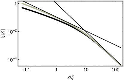
Figure 13: Universal scaling curves on the isotropic line: the black curve represents the longitudinal component $\tilde{X}_{0}$, and the gray curve represents the transverse component $\tilde{X}_{2k_{F}}$. These two single curves were obtained by fitting high order polynomials through the rescaled data set of Figure 12. Thinner straight lines indicate the pure power laws $X(x)\propto 1/x$ and $X(x)\propto 1/x^{2}$.

In Figure 13 we compare the universal scaling functions for the $0k_{F}$ and the $2k_{F}$ components of the cloud, by plotting them on top of each other. We determined the single universal scaling functions by fitting high order polynomials through the scaled data set of Figure 12. We clearly see that the $2k_{F}$ component dominates the $0k_{F}$ component at small $\tilde{x}$, consistent with the known small $x$ asymptotics of Eq. 70.

VIII.4.3 Kondo cloud in the anisotropic case

Having confirmed that the cloud displays the expected universal scaling for isotropic couplings, we move on to the general anisotropic case. The existence of two independent couplings $J_{\parallel}$ and $J_{\perp}$, or equivalently $\alpha$ and $\Delta$, implies that the universal scaling picture is less straightforward. To guide our investigation, let us review known results obtained by an improved poor man’s scaling argument, applicable with greater generality in the anisotropic case. (Standard poor man’s equations (63) can only be trusted when both Kondo exchange couplings are small.)Chakravarty In the language of the spin-boson model, it is known that to leading order in $\Delta$, but arbitrary $\alpha$, increasing the short-distance scale $a$ by $a\,dl$ is approximately equivalent to changing $\alpha$ to $\alpha+d\alpha$ and $\Delta$ to $\Delta+d\Delta$, where

$$\frac{d\alpha}{dl}=-\left(a\Delta\right)^{2}\alpha,~{}~{}~{}\frac{d}{dl}(a\Delta)=(1-\alpha)(a\Delta).$$ (71)

Integration of these flow equations yields scaling trajectories

$$\frac{(a\Delta)^{2}}{2}-\alpha+\ln(\alpha)=\mbox{constant},$$ (72)

or equivalently, in the language of the Kondo model

$$J_{\perp}^{2} -J_{\parallel}^{2}+(2\pi)^{2}\left[\ln\left(1-\frac{J_{\parallel}}{2\pi}\right)+\frac{J_{\parallel}}{2\pi}+\frac{1}{2}\left(\frac{J_{\parallel}}{2\pi}\right)^{2}\right]$$

$$=\mbox{constant}.$$ (73)

A few of these trajectories in the $J_{\parallel}$ - $J_{\perp}$ plane are plotted in Figure 14. We stress that the standard weak coupling renormalization equations (63) cannot be trusted in the regime where $J_{\parallel}\gtrsim 1$, and that is why we have to work non-perturbatively in $\alpha$. It is also important to remember that these trajectories are only meaningful at $J_{\perp}$ sufficiently smaller than $\pi$. Always bearing this proviso in mind, the following statement holds: screening clouds associated with two Kondo Hamiltonians, whose parameters lie on the same scaling trajectory, can be scaled onto the same universal line shape.

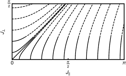
Figure 14: Scaling trajectories that derive from the improved poor man’s scaling equations (71), that are correct to leading order in $J_{\perp}$. In order to emphasize that only the small $J_{\perp}$ part of trajectories are to be trusted, dashed lines are used for $J_{\perp}/2\pi>0.1$.

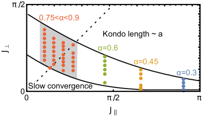
Figure 15: (color online) Map of the parameter space of the Kondo model, where dots indicate points where we have collected data to investigate the scaling behavior of the screening cloud. Below the lower solid curve, $T_{K}\lesssim 10^{-3}/a$ and we generally find that more than $M=7$ coherent states are required for a converged result. Above the upper solid curve, $T_{K}\gtrsim 1/a$ and the screening cloud is poorly resolved because of non-universal ultraviolet effects. At the points included in the shaded region, we find that the screening cloud is nearly isotropic down to distances deep inside the cloud.

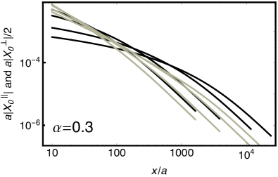
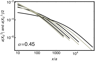
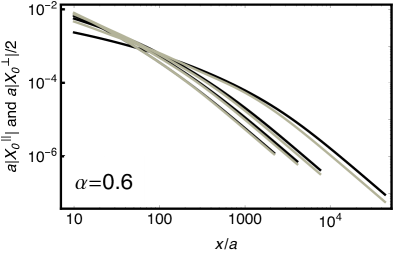
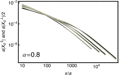
Figure 16: Onset of spin-isotropy in the $0k_{F}$ component of the Kondo cloud, black curves corresponding to the longitudinal correlator $a|X_{0}^{\parallel}|$ and gray curves to the transverse correlator $a|X_{0}^{\perp}|/2$. Top left panel is $\alpha=0.3$, top right panel is $\alpha=0.45$, bottom left panel is $\alpha=0.6$, and bottom right panel is $\alpha=0.8$. In each panel, different curves of the same shade correspond to a few selected values of $\Delta$.

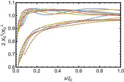
Figure 17: (color online) The ratio $2X_{0}^{\parallel}/X_{0}^{\perp}$ of longitudinal and transverse cloud components plotted against the scaled distance $x/\xi_{\parallel}$. Perfect isotropy corresponds to $2X_{0}^{\parallel}/X_{0}^{\perp}=1$. Solid curves correspond to $\alpha=0.85$ and various values of $\Delta$ ranging from $0.156/a$ to $0.305/a$. Dashed curves correspond to $\alpha=0.75$ and various values of $\Delta$ ranging from $0.120/a$ to $0.268/a$. The Kondo length $\xi_{\parallel}$ was calculated for each curve from Eq. (57). For the set of data at $\alpha=0.85$, $\xi_{\parallel}$ varies from $18.0a$ to $158a$, while for $\alpha=0.75$, $\xi_{\parallel}$ varies from $12.6a$ to $108a$.

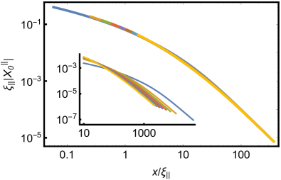
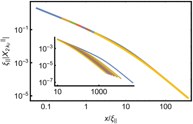
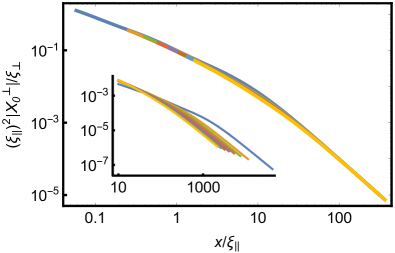
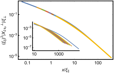
Figure 18: Scaling curves for the four component of the Kondo cloud computed at fixed $\alpha=0.6$ ($J_{\parallel}=1.42$). Raw data is shown in the insets, with different curves correspond to eight different values of $\Delta$ collected in the interval $\Delta\in[0.05/a,0.25/a]$ (i.e. $J_{\perp}\in[0.157,0.785]$). Excellent scaling behavior is obtained for all components.

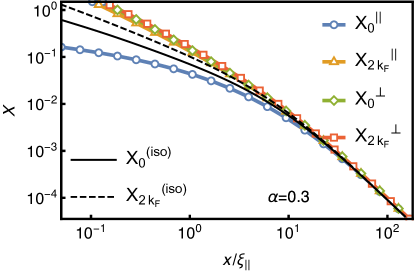
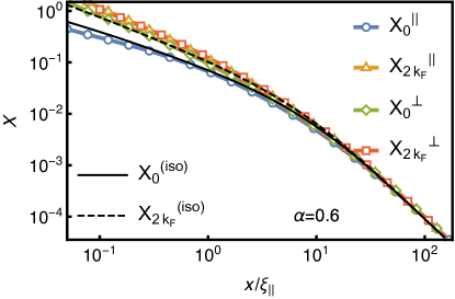
Figure 19: (color online) Comparison between the universal line shapes of the scaled cloud (symbols in color), at $\alpha=0.3$ (top panel) and at $\alpha=0.6$ (bottom panel), to the universal isotropic line shapes (full and dashed black lines). The curves were obtained by fitting data sets such as those displayed in the main panels of Fig. 18 to polynomials of high degree. On the vertical axis, the longitudinal components are plotted in units of $1/\xi_{\parallel}$, while the transverse components are plotted in units of $\xi_{\perp}/\xi_{\parallel}^{2}$. The isotropic curves are those of Figure 13.

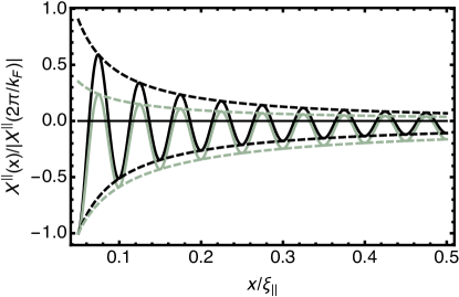
Figure 20: The full longitudinal cloud $X^{\parallel}(x)=X^{\parallel}_{0}(x)+\cos(2k_{F}x)X^{\parallel}_{2k_{F}}(x)$ at $\alpha=0.3$ (black) and on the isotropic line (gray), as shown by full lines (dashed lines are the respective envelope functions $X^{\parallel}_{0}(x)\pm X^{\parallel}_{2k_{F}}(x)$). Both curves were normalized using their magnitude at $x=2\pi/k_{F}$. For the purpose of showing the oscillations, we took $k_{F}=20\pi/\xi_{\perp}$.

Below, our work will be guided by two qualitative features of Figure 14. The first is that the flow trajectories intersect the $J_{\parallel}$-axis at $90^{\circ}$. For large $J_{\parallel}$, the parts of the trajectories that may reasonably be trusted, run nearly parallel to the $J_{\perp}$ axis. Going beyond the small $J_{\perp}$ regime of the figure, we know that, at the Toulouse point $J_{\parallel}=2\pi(1-1/\sqrt{2})$, the scaling trajectory runs exactly parallel to the $J_{\perp}$ axis. (See Appendix D.) Universality at fixed $J_{\parallel}$ is also an obvious feature of the exact analytical expression for the Kondo overlap (62). For $J\gtrsim 0.45\pi$ ($\alpha\leq 0.6$), we will therefore try to scale clouds at fixed $J_{\parallel}$, but different $J_{\perp}$, onto each other.

The second pertinent feature of Figure 14 is that for $J_{\perp},J_{\parallel}\lesssim\pi/2$, trajectories are approximately hyperbolas $J_{\parallel}^{2}-J_{\perp}^{2}=c$. In other words, the isotropic line $J_{\parallel}=J_{\perp}$ is an attractor for the renormalization flow. This implies that at sufficiently large distances $x>x_{\rm iso}$, the cloud must tend to the isotropic cloud. However, for $x<x_{\rm iso}$, the poor man’s scaling picture of Figure 14 indicates pronounced anisotropic behavior. This short distance region corresponds to the scales that have to be integrated out for an anisotropic point $(J_{\parallel},J_{\perp})$ to flow close to the isotropic line. Note, furthermore that the above discussion only applies to points that are in the general vicinity of the isotropic line, and are associated with a Kondo temperature sufficiently lower than $1/a$. If a point is too far from the isotropic line to start with, or if the initial Kondo temperature is too large, the size of the cloud renormalizes down to the ultraviolet scale, before the renormalized couplings become isotropic. At this point the notion of flow trajectories in a two-dimensional parameter space breaks down, and Kondo physics mixes with ultraviolet physics. Based on these observations, we will compare the cloud calculated at $J_{\parallel},J_{\perp}\lesssim\pi/3$ (i.e. reasonably close to the isotropic line and with a decent Kondo length) with the isotropic cloud.

We start the presentation of our results in the regime of small $\alpha$ (large $J_{\parallel}$). This regime does not overlap with the isotropic Kondo regime, because the size of the screening cloud flows to the short distance cut-off $a$ before the renormalized couplings come close to the isotropic line. For small $\alpha$, the single coherent state (Silbey-Harris) approximation is accurate (see Figure 4), and we have derived simple analytical expressions (58) for the cloud correlation functions, that reveal the following universality. By appropriately rescaling the four cloud components and the coordinate $x$, clouds calculated at different $J_{\perp}\ll\pi$ but fixed $J_{\parallel}$ (i.e. fixed $\alpha$) have the same line shape: For the longitudinal components $X_{j}^{\parallel}$, $j\in\{0,2k_{F}\}$ one defines

$$\tilde{X}_{j}^{\parallel}(\alpha,\tilde{x})=\xi_{\parallel}X_{j}(x),~{}~{}~{}\tilde{x}=x/\xi_{\parallel},$$ (74)

and finds from the Silbey-Harris result the simple analytical formulas:

$$\tilde{X}_{0}^{\parallel}(\alpha,\tilde{x}) =-{\rm Re}\,F\left(\frac{i\sqrt{\alpha}\tilde{x}}{\pi}\right),$$

$$\tilde{X}_{2k_{F}}^{\parallel}(\alpha,\tilde{x}) =-\frac{1}{2\pi\tilde{x}}\sin\left[2\sqrt{\alpha}{\rm Im\,}F\left(\frac{i\sqrt{\alpha}\tilde{x}}{\pi}\right)\right].$$ (75)

In the small $\alpha$ regime, the two transverse components $X_{j}^{\perp}$, $j\in\{0,2k_{F}\}$, are equal. One defines

$$\tilde{X}_{j}^{\perp}(\alpha,\tilde{x})=\xi_{\parallel}^{2}X_{j}(x)/\xi_{\perp},~{}~{}~{}\tilde{x}=x/\xi_{\parallel},$$ (76)

and finds the analytical expression:

$$\tilde{X}_{j}^{\perp}(\alpha,\tilde{x})=-\frac{2}{\tilde{x}^{2}}\exp\left[-2\sqrt{\alpha}{\rm Re\,}F\left(\frac{i\sqrt{\alpha}\tilde{x}}{\pi}\right)\right].$$ (77)

The expression for $\tilde{X}_{0}^{\parallel}(x)$ could suggest a further rescaling $\bar{x}=\sqrt{\alpha}\tilde{x}$ that would lead to an $\alpha$ independent line shape for $X_{0}^{\parallel}$. However, one cannot simultaneously get rid of the $\alpha$ dependence in the other components of the cloud. Furthermore, it turns out that $\tilde{X}^{\parallel}(\alpha,z/\sqrt{\alpha})$ is no longer $\alpha$-independent beyond $\alpha\gtrsim 0.4$ (as shown by our numerical simulations below).

The two pertinent facts to emerge from this discussion are the following. Firstly, whereas the magnitudes of the longitudinal and transverse components of the cloud have to be rescaled by different inverse lengths $1/\xi_{\parallel}$ and $\xi_{\perp}/(\xi_{\parallel})^{2}$, the coordinate $x$ is always rescaled by $\xi_{\parallel}$. In other words, the longitudinal and transverse clouds have different characteristic magnitudes $1/\xi_{\parallel}$ and $\xi_{\perp}/(\xi_{\parallel})^{2}$, but the same characteristic size $\xi_{\parallel}$. Secondly, the universal scaling curves depend in general on $\alpha$. Thus, as expected from poor man’s scaling, clouds at the same $J_{\parallel}$ but different $J_{\perp}$ have the same shape, whereas clouds at different $J_{\parallel}$ in general have different shapes.

The differences in scaling behavior between the small $\alpha$ and isotropic clouds are thrown into sharp relief when one considers the small $x$ asymptotic form of the cloud correlators. At $\tilde{x}\ll 1$, the small $\alpha$ results (75) and (77) lead to asymptotic behavior:

$$\tilde{X}^{\perp}_{0}=\tilde{X}^{\perp}_{2k_{F}}\sim-\tilde{x}^{-2(1-\sqrt{\alpha})},$$

$$\tilde{X}_{0}^{\parallel}\sim\ln\tilde{x},~{}~{}~{}\tilde{X}_{2k_{F}}^{\parallel}\sim-\tilde{x}^{-1}.$$ (78)

The $\tilde{X}_{0}^{\parallel}$ component diverges much more slowly in the $\tilde{x}\to 0$ limit than is the case at isotropic couplings ($\ln\tilde{x}$ vs. $-1/\tilde{x}(\ln\tilde{x})^{2}$), whereas the $\tilde{X}_{2k_{F}}^{\parallel}$ component diverges more rapidly than in the isotropic case ($-1/\tilde{x}$ vs. $1/\tilde{x}\ln\tilde{x}$). Thus, the alternation between ferro- and antiferromagnetic correlations close to the impurity is enhanced in the longitudinal direction. This is not surprising, as small $\alpha$ implies $J_{\parallel}\gg J_{\perp}$. Furthermore we see that the small $x$ asymptotic behavior of the transverse cloud is explicitly $\alpha$-dependent, displaying power-law behavior with an exponent $-2(1-\sqrt{\alpha})=-J_{\parallel}/\pi$, implying a divergence as $\tilde{x}\to 0$ that is closer to $1/x^{2}$, than to $1/x$.

The next obvious question is how the small $\alpha$ scaling picture evolves as $\alpha$ increases. In order to investigate this, we calculated the cloud correlators at the points in parameter space shown in Figure 15. The most obvious feature of the data, is that the cloud becomes more and more isotropic as $\alpha$ increases. This is revealed in Figure 16, where we plot $X_{0}^{\parallel}(x)$ and $X_{0}^{\perp}(x)/2$ on top of each other for respectively $\alpha=0.3$, $\alpha=0.45$, $\alpha=0.6$, and $\alpha=0.8$, in separate panels. Each panel contains curves for several values of $J_{\perp}$. At $\alpha=0.3$, the transverse and longitudinal clouds are very different. As $\alpha$ increases, the differences become smaller. By the time we reach $\alpha=0.8$, the cloud is isotropic to a high degree of accuracy for all values of $J_{\perp}$ considered. The behavior of the $X_{2k_{F}}^{\parallel}(x)$ and $X_{2k_{F}}^{\perp}(x)$ components of the cloud (not shown) present very similar behavior. We find similarly isotropic clouds at all the points in Figure 15 inside the shaded region.

Poor man’s scaling suggests that for anisotropic exchange couplings, there is a scale $x_{\rm iso}$ below which isotropy breaks down. To investigate this, we plot the ratio $2X_{0}^{\parallel}/X_{0}^{\perp}$ as a function of $x/\xi_{\parallel}$ (Figure 17). We do so for the data collected at $\alpha=0.75$ and for $\alpha=0.85$. In both cases we see that $2X_{0}^{\parallel}/X_{0}^{\perp}$ reaches a plateau that is within 10% of unity. This is the same degree of isotropy as we obtain on the isotropic line itself. In both cases, the plateau is reached at a distance that is a small fraction of the Kondo length $\xi_{\perp}$. In other words, isotropy extends deep inside the cloud. The ratio $x_{\rm iso}/\xi_{\parallel}$ between the scale where isotropy sets in, and the Kondo length, is more or less constant at fixed $\alpha$, while the Kondo length itself varies by an order of magnitude. From the figure one can read off that $x_{\rm iso}/\xi_{\parallel}\sim 0.2$ for $\alpha=0.75$ and $x_{\rm iso}/\xi_{\parallel}\sim 0.05$ for $\alpha=0.85$.

Next, we investigate the precise scaling behavior of the data. For $\alpha\leq 0.6$, we take our cue from the small $\alpha$ results we obtained above, together with the understanding from poor man’s scaling, and we thus scale correlation functions according to the Ansatz (74) and (76). In Fig. 18, we show raw and scaled results for $\alpha=0.6$. Similar figures for $\alpha=0.3$ and $0.45$ can be found in the supplementary material.supmat For all values of $\alpha$ that we considered, the data nicely scale onto single universal curves. We conclude that for practical purposes, scaling Ansatz of the form (74) and (76) hold for all values of $\alpha<0.6$.

These universal scaling curves are $\alpha$-dependent and differ from the isotropic scaling curves. This can clearly be seen in Figure 19, where we compare the universal line shapes of the scaled cloud at $\alpha=0.3$ (top panel) and at $\alpha=0.6$ (bottom panel) to the universal isotropic line shapes obtained in Sec. VIII.4.2. Although the single coherent state (Silbey-Harris) approximation underestimates the Kondo length $\xi_{\parallel}$ by $50\%$ at $\alpha=0.3$, the simple equations (75-77) still predict the universal line shape of the screening cloud very well. Inside the cloud ($x<\xi_{\parallel}$), these universal curves are very different from the universal isotropic curves. As $\alpha$ increases, deviations from the Silbey-Harris line-shape set in, and scaling curves start to resemble the isotropic curves more closely, as can be seen for $\alpha=0.6$ in the bottom panel of Figure 19.

A prominent feature of the anisotropic scaling curves is that, at small distances, there is a stronger suppression of the $X_{0}^{\parallel}$ component over the $X_{2k_{F}}^{\parallel}$ component, than in the isotropic case. As a result, the alternation from ferro- to antiferromagnetic correlations between the impurity and the electron gas inside the cloud is enhanced in the longitudinal direction. This is illustrated in Figure 20, where we compare the full longitudinal cloud $X^{\parallel}(x)=X^{\parallel}_{0}(x)+\cos(2k_{F}x)X^{\parallel}_{2k_{F}}(x)$ calculated at $\alpha=0.3$ with the result on the isotropic line.

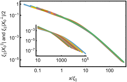
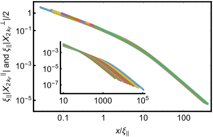
Figure 21: (color online) The screening cloud calculated at all points inside the shaded region ($0.75\leq\alpha\leq 0.9$) in Figure 15. Insets show the raw data, while the main panels show data in units of $\xi_{\parallel}$ on the horizontal axis and units of $1/\xi_{\parallel}$ on the vertical axis. The top panel contains the transverse and longitudinal $0k_{F}$ components plotted together. The bottom panel contains the transverse and longitudinal $2k_{F}$ components.

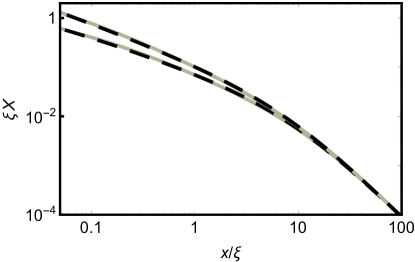
Figure 22: The solid gray curves represent the (isotropic) universal scaling curves inferred using all the data of Figure 21, i.e. clouds calculated at all the points inside the shaded region in Figure 15. These curves were obtained as the best fit of a high order polinomial through the scaled data of Figure 21. The dashed black curves are the universal scaling curves inferred using only clouds calculated at perfectly isotropic couplings (See Figure 13).

To complete the scaling analysis, we consider the screening cloud at $0.75\leq\alpha\leq 0.9$ (the shaded region in Figure 15). In this region, we have seen that the cloud is approximately isotropic. In Figure 21, we therefore plot the transverse and longitudinal components of the cloud on the same graph. Insets show raw results in units of $a$ on the horizontal and $1/a$ on the vertical axes. The main panels show data in rescaled units of $\xi_{\parallel}$ on the horizontal and $1/\xi_{\parallel}$ on the vertical axes. We see that the scaled data collapse very well onto single scaling curves. As before, the Kondo length $\xi_{\parallel}$ was calculated using Eq. (57), i.e. no fitting parameters were used to obtain the high degree of collapse. It is instructive to compare the main panels of Figure 21 for all the data collected, to Figure 12, that shows scaled data only for the subset of points that lie on the isotropic line $J_{\perp}=J_{\parallel}$. We see the same degree of collapse onto single curves in both figures. In other words, within the numerical accuracy of our calculation, the universal line shape of the screening cloud is the same for all points in the shaded region of Figure 15. To further confirm this conclusion, we fitted a high order polynomial through the complete scaled data sets of Figure 21. In Figure 22 we compare this fit to the universal scaling curves we obtained previously by only considering the cloud on the isotropic line (Figure 13). We see nearly perfect agreement. Of course, the screening cloud at an anisotropic value of the exchange couplings, $J_{\perp}\not=J_{\parallel}$, only follows this universal line shape for distances larger than $x_{\rm iso}$, the scale at which isotropy sets in. However, as we have seen in Figure 17, there is a sizable region around the isotropic line where isotropy already sets in deep inside the cloud.

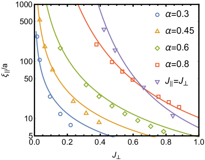
Figure 23: (color online) The Kondo length $\xi_{\parallel}$ as a function of $J_{\perp}$ for several $\alpha$ values. The solid lines shows $\xi=c/T_{K}$, with $T_{K}$ the standard poor man’s scaling estimate (64) and $c$ a fitting parameter. The same value of $c=0.3$ we used for all five curves.

Finally, we plot in Figure 23 the Kondo length $\xi_{\parallel}$, which corresponds to the characteristic size of the cloud, for some of the data we have collected. The large range over which $\xi_{\parallel}$ varies for each value of $\alpha$, confirms that the scaling behavior we see is non-trivial. We compare the calculated value of $\xi_{\parallel}$ to $\xi\propto 1/T_{K}$, with $T_{K}$ the standard poor man’s scaling estimate (64) of the Kondo temperature. With a logarithmic scale on the vertical axis, which hides mismatches by factors of order unity, we find good agreement for the isotropic and the $\alpha=0.8$ data sets. That these sets yield the best agreement is expected, as they are closer to the point $J_{\perp}=J_{\parallel}=0$ in parameter space than the other sets, and the version of poor man’s scaling that leads to the estimate (64) for $T_{K}$ assumes small exchange couplings.

IX Summary of results and conclusion

This paper has provided a very extensive study of the Kondo screening cloud for a wide range of parameter values, including the spin-isotropic and strongly spin-anisotropic regimes. Methodologically, we derived simple but controlled analytical expressions in the case of strong anisotropy, and developed an original and very powerful numerical technique to tackle the problem in its complete generality. This allowed us to investigate the $0k_{F}$ and $2k_{F}$ component of the Kondo cloud correlator separately, both for the longitudinal and transverse response. In addition, we have examined, again both analytically and numerically, the structure of Kondo overlaps introduced in recent works.luk

Our main results concern the universal scaling of correlations between the impurity spin and the electron spin density in the anisotropic Kondo model. They can be summarized as follows. At large $x$, transverse correlators equal $X_{k}^{\perp}(x)=-\xi_{\perp}/x^{2}$ while longitudinal correlators equal $X_{k}^{\parallel}(x)=-\xi_{\parallel}/x^{2}$ (here $k=0,\,2k_{F}$ refer to respectively the forward or backscattering component of the correlator). In general, the two emergent length scales $\xi_{\perp}$ and $\xi_{\parallel}$ are not equal, and we find the following universal scaling behavior:

$$X_{k}^{\perp}(x)=\frac{\xi_{\perp}}{\xi_{\parallel}^{2}}\tilde{X}_{k}^{\perp}(\alpha,x/\xi_{\parallel}),$$

$$X_{k}^{\parallel}(x)=\frac{1}{\xi_{\parallel}}\tilde{X}_{k}^{\parallel}(\alpha,x/\xi_{\parallel}).$$ (79)

The scaling curves are $J_{\perp}$-independent, but remain $\alpha$-dependent (and therefore $J_{\parallel}$-dependent). As can be seen from the scaling equations, the two lengths $\xi_{\perp}$ and $\xi_{\parallel}$ have fundamentally different roles. The length $\xi_{\parallel}$ sets the size of the screening cloud, whereas the ratio $\xi_{\perp}/\xi_{\parallel}$ sets the relative magnitude of transverse correlations, compared to longitudinal correlations.

As $J_{\parallel}$ decreases, the explicit $J_{\parallel}$ dependence of the scaling curves becomes weaker and weaker. For $J_{\parallel}\ll 1$, we find no discernible $J_{\parallel}$-dependence anymore, and the universal scaling curves become those of the isotropic model. In this region of parameter space, we find that isotropy already sets in deep inside the cloud. We managed to calculate the universal scaling curves down to distances $x/\xi=0.1$ or less. This far inside the cloud, the backscattering ($2k_{F}$) component of the longitudinal correlator dominates the forward scattering ($0k_{F}$) component. Inside the cloud, correlations between the impurity spin and the electron spin density therefore alternate with wave vector $2k_{F}$ between being ferro- and antiferromagnetic. The effect is more pronounced in the regime $J_{\parallel}\gg J_{\perp}$, but we can still clearly resolve it when the cloud becomes isotropic.

In previous numerical studies, results were obtained using the numerical renormalization group (NRG). This required solving a two-impurity problem, where the position of the second (fictitious) impurity represents the point $x$ where the correlator is evaluated. An independent two channel Kondo problem must be solved by NRG at every position where the correlator is evaluated, making the calculation computationally expensive. In addition, it proved difficult to resolve in NRG the dominance of the backscattering components of the cloud over the forward scattering components inside the cloud.

We have shown that the coherent state expansion, the method we employed in this Article, complements previous numerical renormalization group studies, and even offers simple analytical insights in the regime of strong spin-anisotropy. Thanks to a technical improvement that dramatically reduces the number of variational parameters, it offers excellent accuracy at a reduced computational cost, and does not require one to discretize the bath degrees of freedom. Yet, we note that the numerical renormalization group was successfully used to study finite temperature Borda and time-dependentLechtenberg features of the Kondo cloud. We envisage future work to extend the coherent state expansion into these domains as well.

Appendix A Mapping between the Kondo and Spin-Boson Models

In this Appendix, we review the mapping from the Kondo Hamiltonian (3) to the spin-boson Hamiltonian (5). The first step is to express the (even) fermionic degrees of freedom in terms of bosonic ones $b_{q\sigma}$, $q=2\pi n/L$, $n\in\{1,\,2,\,3,\,\ldots\}$ with $[b_{q\sigma},b_{q^{\prime}\sigma^{\prime}}^{\dagger}]=\delta_{qq^{\prime}}\delta_{\sigma\sigma^{\prime}}$. For this purpose, we invoke the bosonization identities

$$b_{q\sigma}=\sqrt{\frac{2\pi}{Lq}}\int_{-L/2}^{L/2}dx\,e^{-iqx}\psi^{\dagger}_{\sigma}(x)\psi_{\sigma}(x),$$ (80)

and

$$\psi^{\dagger}_{\sigma}(x)=\frac{F^{\dagger}_{\sigma}}{\sqrt{2\pi a}}e^{-i\phi_{\sigma}(x)},$$

$$\phi_{\sigma}(x)=i\sum_{q>0}\sqrt{\frac{2\pi}{qL}}e^{-(a/2+ix)q}b_{q\sigma}^{\dagger}+\mbox{h.c.}.$$ (81)

Here $F_{\sigma}^{\dagger}$ denotes the unitary Klein factor operator associated with increasing the number of $\sigma$ electrons by one.

We separate spin and charge degrees of freedom by defining:

$$a_{q}=(b_{q\uparrow}+b_{q\downarrow})/\sqrt{2},~{}~{}~{}b_{q}=(b_{q\uparrow}-b_{q\downarrow})/\sqrt{2}.$$ (82)

We also define new SU(2) operators, in which fermion number and impurity degrees of freedom are mixed.

$$s^{-}=F^{\dagger}_{\uparrow}F_{\downarrow}\sigma^{-},~{}~{}~{}s^{+}=(s^{-})^{\dagger},~{}~{}~{}s_{z}=\sigma_{z}.$$ (83)

In the bosonic representation, the Hamiltonian reads

$$H_{0}=\sum_{q>0}q(a_{q}^{\dagger}a_{q}+b_{q}^{\dagger}b_{q}),$$

$$H_{\parallel}=\frac{J_{\parallel}}{2}\sum_{q>0}\sqrt{\frac{q}{\pi L}}e^{-aq/2}(b_{q}^{\dagger}+b_{q})s_{z},$$

$$H_{\perp}=\frac{J_{\perp}}{2\pi a}\left[e^{-\sqrt{2}i\phi}s^{-}+e^{\sqrt{2}i\phi}s^{+}\right],$$ (84)

where

$$\phi =\frac{\phi_{\uparrow}(0)-\phi_{\downarrow}(0)}{\sqrt{2}}=i\sum_{q>0}\sqrt{\frac{2\pi}{Lq}}e^{-aq/2}(b_{q}^{\dagger}-b_{q}).$$ (85)

We note that spin ($b_{q}$) and charge ($a_{q}$) degrees of freedom are decoupled, and that only spin degrees of freedom couple to the impurity. We restrict the Hamiltonian to the vacuum of the charge sector and drop the $a^{\dagger}a$ terms in future expressions.

Finally, we bring the Hamiltonian into the standard form of the (unbiased) spin-boson model, via a unitary transform

$$U=\exp(-is_{z}\phi/\sqrt{2}).$$ (86)

Under the action of $U$,

$$Ub_{q}U^{\dagger}=b_{q}-\sqrt{\frac{\pi}{Lq}}e^{-aq/2}s_{z},~{}~{}~{}Us^{-}U^{\dagger}=e^{\sqrt{2}i\phi}s^{-},$$ (87)

so that $UHU^{\dagger}=H_{\rm SB}+\mbox{const}$, where $H_{\rm SB}$ is given by (5).

Appendix B Correlation functions in the bosonic representation

In this Appendix, we transform the fermionic cloud correlators (7) onto their bosonic counterparts (10). To do so, we represent the electron spin density in terms of bosonic degrees of freedom, and subsequently perform the unitary transformation of (86) on these operators. To this end, it is useful to note from (4) the following identities:

$$\frac{1}{\sqrt{2}}\left[\tilde{\psi}_{\sigma}(x)+\tilde{\psi}_{\sigma}(-x)\right]\simeq e^{ik_{F}x}\psi_{\sigma}(x)+e^{-ik_{F}x}\psi_{\sigma}(-x),$$

$$\frac{1}{\sqrt{2}}\left[\tilde{\psi}_{\sigma}(x)-\tilde{\psi}_{\sigma}(-x)\right]\simeq e^{ik_{F}x}\bar{\psi}_{\sigma}(x)-e^{-ik_{F}x}\bar{\psi}_{\sigma}(-x).$$ (88)

The ‘approximately equal’ signs in these equations indicate that the operators on the right hand side represent versions of the point operators on the left, that have been broadened by an amount $\sim a$, inversely proportional to the ultraviolet cut-off. Now consider the expectation value $X^{\perp}(x)$, which, from (7), can also be written as

$$X^{\perp}(x)=4{\rm Re}\left<\sigma^{-}\tilde{\psi}^{\dagger}_{\uparrow}(x)\tilde{\psi}_{\downarrow}(x)\right>_{\rm K}.$$ (89)

Because the ground state has good spatial parity, $X^{\perp}(x)$ is an even function, and we may write

$$X^{\perp}(x)=2{\rm Re}\left<\sigma^{-}\left[\tilde{\psi}^{\dagger}_{\uparrow}(x)\tilde{\psi}_{\downarrow}(x)+\tilde{\psi}^{\dagger}_{\uparrow}(-x)\tilde{\psi}_{\downarrow}(-x)\right]\right>_{\rm K}.$$ (90)

The last expression is manipulated to become

$$X^{\perp}(x)={\rm Re}\left\{\left<\sigma^{-}\left[\tilde{\psi}^{\dagger}_{\uparrow}(x)+\tilde{\psi}^{\dagger}_{\uparrow}(-x)\right]\left[\tilde{\psi}_{\downarrow}(x)+\tilde{\psi}_{\downarrow}(-x)\right]\right>_{\rm K}+\underbrace{\left<\sigma^{-}\left[\tilde{\psi}^{\dagger}_{\uparrow}(x)-\tilde{\psi}^{\dagger}_{\uparrow}(-x)\right]\left[\tilde{\psi}_{\downarrow}(x)-\tilde{\psi}_{\downarrow}(-x)\right]\right>_{\rm K}}_{=0}\right\}.$$ (91)

The term marked with the underbrace is zero because of the following reason: $\tilde{\psi}^{\dagger}_{\uparrow}(x)-\tilde{\psi}^{\dagger}_{\uparrow}(-x)$ creates an electron in an odd parity single particle orbital, and these orbitals do not couple to the impurity, so that:

$$\left<\sigma^{-}\left[\tilde{\psi}^{\dagger}_{\uparrow}(x)-\tilde{\psi}^{\dagger}_{\uparrow}(-x)\right]\left[\tilde{\psi}_{\downarrow}(x)-\tilde{\psi}_{\downarrow}(-x)\right]\right>_{\rm K}=\left<\sigma^{-}\right>_{\rm K}\left<\left[\tilde{\psi}^{\dagger}_{\uparrow}(x)-\tilde{\psi}^{\dagger}_{\uparrow}(-x)\right]\left[\tilde{\psi}_{\downarrow}(x)-\tilde{\psi}_{\downarrow}(-x)\right]\right>_{\rm K}.$$ (92)

Since the antiferromagnetic Kondo ground state is a singlet, $\left<\sigma^{-}\right>_{\rm K}=0$. Substituting from (88) into the first line of (91), we obtain

$$X^{\perp}(x)=2{\rm Re}\left<\sigma^{-}\left[\psi^{\dagger}_{\uparrow}(x)\psi_{\downarrow}(x)+\psi^{\dagger}_{\uparrow}(-x)\psi_{\downarrow}(-x)+e^{-2ik_{F}x}\psi^{\dagger}_{\uparrow}(x)\psi_{\downarrow}(-x)+e^{2ik_{F}x}\psi^{\dagger}_{\uparrow}(-x)\psi_{\downarrow}(x)\right]\right>_{\rm K}.$$ (93)

Performing a similar calculation for $X^{\parallel}(x)$, we find

$$X^{\parallel}(x)=\frac{1}{2}\sum_{\sigma}{\rm sgn}(\sigma)\left<\sigma_{z}\left[\psi^{\dagger}_{\sigma}(x)\psi_{\sigma}(x)+\psi^{\dagger}_{\sigma}(-x)\psi_{\sigma}(-x)+e^{-2ik_{F}x}\psi^{\dagger}_{\sigma}(x)\psi_{\sigma}(-x)+e^{2ik_{F}x}\psi^{\dagger}_{\sigma}(-x)\psi_{\sigma}(x)\right]\right>_{\rm K},$$ (94)

where ${\rm sgn}(\uparrow)=+$ and ${\rm sgn}(\downarrow)=-$. We finally manipulate the above expressions as follows:

1. The fermion operators are bosonized.

2. We apply the unitary transformation that maps the Kondo Hamiltonian onto the spin-boson model. In the resulting expressions, expectation values are with respect to the ground state of the spin-boson model, indicated without a subscript.

3. We normal order the bosonic operators. In the resulting expressions, the operators $a_{q}^{\dagger}$ and $a_{q}$, are replaced by zeros, since $a_{q}$ annihilates the ground state.

Finally, we take the large system limit, which allows us to make replacements such as $1-e^{-(a+ix)2\pi/L}\to 2\pi(a+ix)/L$. The resulting expressions are those presented in the main text (10).

Appendix C Contour integral for cloud calculation

The integrals involved in calculating the cloud are of the form:

$$\int_{0}^{\infty}dqe^{-(a\pm ix)q}r(q),$$ (95)

where the function $r(q)$ goes to zero as least as fast as $1/q$ for large $q$. Furthermore, the only non-analyticities that $r(q)$ possesses in the complex $q$ plane are (first order) poles at $\omega_{n}$, $n=1,\,\ldots,\,M$. These integrals can be performed by extending the method employed in Sec. VI, where the energy was calculated.

Define $z=a\pm ix$ and $\theta=-{\rm arg}(z)$. Integrating around the shaded area $A$, whose azimuthal boundary is understood to lie at $|q|\to\infty$ in Figure 24, we obtain

$$\int_{0}^{\infty}dq\,e^{-zq}r(q)=e^{i\theta}\int_{0}^{\infty}dp\,e^{-|z|p}r(pe^{i\theta})$$

$$+2\pi i\sum_{\omega_{n}\in A}{\rm Res}\left[e^{-zq}r(q),\omega_{n}\right].$$ (96)

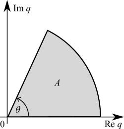
Figure 24: Integration contour used in Appendix C.

The integral on the right hand side on the first line is of precisely the same form as those considered in Sec. VI. We also note that the summation on the second line vanishes if there are no poles $\omega_{n}$ with positive real parts. Using the results of Sec. VI, we obtain:

$$\int_{0}^{\infty}dq\,e^{-zq}r(q)=\sum_{m=1}^{N}{\rm Res}\left[e^{-zq}E_{1}(-zq)r(q),\omega_{n}\right]$$

$$+2\pi i\sum_{\omega_{n}\in A}{\rm Res}\left[e^{-zq}r(q),\omega_{n}\right].$$ (97)

Appendix D Exact results at the Toulouse point

In this appendix, we review the mapping between the Kondo model at the Toulouse point $\alpha=1/2$ (i.e. $J_{\parallel}=2\pi(1-1/\sqrt{2})$), and the non-interacting fermionic resonant level model, following Ref. Zarand, . We also derive an exact expression for the longitudinal $0k_{F}$ component of the screening cloud. The derivation takes the same route as that set out in Refs. Posske1, and Posske2, .

The starting point is the bosonic representation (84) of the Kondo hamiltonian. The fermionic non-interacting resonant level $H_{\rm rlm}$ is obtained, by applying the unitary transform $H_{\rm rlm}=U^{\prime}H(U^{\prime})^{\dagger}$, where

$$U^{\prime}=\exp\left\{i\sigma_{z}\left[\frac{\pi}{2}N_{-}-\left(1-\frac{1}{\sqrt{2}}\right)\frac{\phi}{\sqrt{2}}\right]\right\}.$$ (98)

The bosonic field $\phi$ is defined in Eq. (85), and the operator

$$N_{-}=(N_{\uparrow}-N_{\downarrow})/2,$$ (99)

is the $z$-component of the total spin of the electron gas. New degrees of freedom

$$\bar{\psi}(x)^{\dagger} = \exp\left[-\frac{2\pi i}{L}\left(N_{-}-\frac{1}{2}\right)x-i\phi(x)\right]\frac{F_{\uparrow}^{\dagger}F_{\downarrow}}{\sqrt{2\pi a}}$$

$$= \frac{1}{\sqrt{L}}\sum_{k}e^{-ikx}e^{-a|k|/2}\bar{c}_{k}^{\dagger}$$

$$d^{\dagger} = \exp\left[i\pi\left(N_{-}\frac{1}{2}\right)\right]\sigma^{+},$$ (100)

emerge, that obey the usual fermionic commutation relations. Here

$$\phi(x)=\frac{\phi_{\uparrow}(x)-\phi_{\downarrow}(x)}{\sqrt{2}},$$ (101)

with $\phi_{\uparrow(\downarrow)}(x)$ defined in Eq. (81), and $F_{\uparrow(\downarrow)}^{\dagger}$ denote Klein factors. In terms of these new fermions, $H_{\rm rlm}$ reads

$$H_{\rm rlm}=\sum_{q}q\bar{c}_{q}^{\dagger}\bar{c}_{q}+\frac{J_{\perp}}{\sqrt{2\pi a}}\left[\bar{\psi}(x)^{\dagger}d+d^{\dagger}\bar{\psi}(x)\right].$$ (102)

At the Toulouse point, the unitary transformation $U^{\prime}$ maps the ground state of the Kondo Hamiltonian onto the ground state of $H_{\rm rlm}$. Since $H_{\rm rlm}$ is a quadratic Hamiltonian, ground state correlation functions can be calculated straight-forwardly for transformed observables, provided they are expressed simply in terms of the new fermionic degrees of freedom. Here we focus on the longitudinal $0k_{F}$ component $X_{0}^{\parallel}$ for which this is easily accomplished.

Applying the unitary mapping to the $z$-components of the impurity spin and the electron spin density operators, one finds

$$X_{0}^{\parallel}(x)= \sqrt{2}\left<\left(d^{\dagger}d-\frac{1}{2}\right)\left[\bar{\psi}(x)^{\dagger}\bar{\psi}(x)+\bar{\psi}(-x)^{\dagger}\bar{\psi}(-x)\right]\right>$$

$$-(2-\sqrt{2})\frac{a}{x^{2}+a^{2}},$$ (103)

where the expectation value on the right hand side of the first line is with respect to the ground state of $H_{\rm rlm}$. This expression is further simplified using Wick’s theorem and noting that the occupation probability for the resonant level is one half, i.e. $\left<d^{\dagger}d\right>=1/2$. In terms of the original degrees of freedom, this corresponds to $\left<\sigma_{z}\right>=0$ which is guaranteed by the singlet nature of the Kondo ground state. Working directly with $H_{\rm rlm}$, this follows from particle-hole symmetry. (Note that the energy of the resonant level co-incides with the Fermi energy.) To be more precise, $H_{\rm rlm}$ is invariant under the combined action of particle-hole and spatial inversion. Owing to the same symmetry, $\left<d^{\dagger}\bar{\psi}(x)\right>=\left<d^{\dagger}\bar{\psi}(-x)\right>^{*}$. Putting everything together, one obtains

$$X_{0}^{\parallel}(x)=-2\sqrt{2}\left|\left<d^{\dagger}\bar{\psi}(x)\right>\right|^{2}-(2-\sqrt{2})\frac{a}{x^{2}+a^{2}}.$$ (104)

The expectation value $\left<d^{\dagger}\bar{\psi}(x)\right>$ can be calculated from the known single particle Green’s functions of the resonant level model. In the thermodynamic limit ($L\to\infty$) the exact result is

$$\left<d^{\dagger}\bar{\psi}(x)\right>$$

$$=\frac{J_{\perp}}{\sqrt{2\pi a}}\int_{-\infty}^{0}\frac{d\omega}{2\pi}e^{i\omega x}\left[\frac{\theta_{R}(x)}{\omega-\Sigma(\omega)}-\frac{\theta_{R}(-x)}{\omega-\Sigma(\omega)^{*}}\right],$$ (105)

where $\theta_{R}(x)$ is a regularized step function

$$\theta_{R}(x)=i\int_{-\infty}^{\infty}\frac{dk}{2\pi}\frac{e^{i(k-\omega)x-a|k|}}{\omega^{+}-k}$$

$$=e^{\omega a}\left[\theta(x)+\frac{i\Gamma(0,\omega(ix+a))}{2\pi}\right]-e^{-\omega a}\frac{i\Gamma(0,\omega(ix-a))}{2\pi},$$ (106)

with $\omega^{+}=\omega+i0^{+}$, and $\Sigma(\omega)$ is the retarded resonant level self-energy

$$\Sigma(\omega)=\frac{J_{\perp}^{2}}{4\pi^{2}a}\int_{-\infty}^{\infty}dk\,\frac{e^{-a|k|}}{\omega^{+}-k},$$

$$=\frac{J_{\perp}^{2}}{4\pi^{2}a}\left[e^{a\omega}\Gamma(0,a\omega^{+})-e^{-a\omega}\Gamma(0,-a\omega^{+})\right].$$ (107)

In general, the integral (105) has to be evaluated numerically. However, for $|x|\gg a$, the following approximations are valid, which yields an analytical result. As a function of (negative) $\omega$, the regularized step function $\theta_{R}(x)$ is suppressed as $e^{\omega a}$ for $x>0$. As a result, the integrand of (105) is strongly suppressed for $-\omega\gtrsim 1/a$. As a function of $x$, the regularized step function is smoothed at a scale $|x|\lesssim a$. For $-\omega<1/a$ and $|x|\gg a$, the regularized step function can be replaced with the sharp step function $\theta(x)$. For $x\gg a$, the rapidly oscillating factor $e^{i\omega x}$ then cuts off the integral at $\omega\sim 1/x\ll 1/x$, so that the self-energy $\Sigma(\omega)$, that varies on the scale of $1/a$, can be evaluated at $\omega=0$

$$\Sigma(0)=-\frac{iJ_{\perp}^{2}}{4\pi a}.$$ (108)

For $|x|\gg a$, one then finds

$$\left<d^{\dagger}\bar{\psi}(x)\right> =\frac{J_{\perp}}{\sqrt{2\pi a}}\int_{-\infty}^{0}\frac{d\omega}{2\pi}\frac{e^{i\omega|x|}}{\omega+i\frac{J_{\perp}^{2}}{4\pi a}}$$

$$=-\frac{J_{\perp}}{\sqrt{2\pi a}}\frac{F\left(-\frac{J_{\perp}^{2}|x|}{4\pi a}\right)}{2\pi},$$ (109)

where $F(z)$ is defined in Eq. (38). We substitute this into (104) and also drop the second term in that equation, which is valid for $|x|\gg a$, to obtain

$$X_{0}^{\parallel}(x)=-\frac{\sqrt{2}}{\pi^{2}}\frac{J_{\perp}^{2}}{4\pi a}F\left(-\frac{J_{\perp}^{2}|x|}{4\pi a}\right)^{2}.$$ (110)

The Kondo length $\xi_{\parallel}$ is defined as in (56) in the main text, i.e. $\xi_{\parallel}=\lim_{x\to\infty}x^{2}X_{0}^{\parallel}(x)$. This yields

$$\xi_{\parallel}=\frac{\sqrt{2}}{\pi^{2}}\frac{4\pi a}{J_{\perp}^{2}},$$ (111)

and a universal scaling function (cf. Eq. (74))

$$\tilde{X}^{\parallel}_{0}(\alpha=1/2,\tilde{x})=-\frac{2}{\pi^{4}}F\left(-\frac{\sqrt{2}\tilde{x}}{\pi^{2}}\right)^{2}.$$ (112)

Supplementary information for “Universal spatial correlations in the anisotropic Kondo screening cloud: analytical insights and numerically exact results from a coherent state expansion”

Scaling analysis of the anisotropic cloud

In the main text, we showed extensive data at $\alpha=0.6$ (i.e. $J_{\parallel}=1.42$) demonstrating that cloud correlation functions calculated at different values of $\Delta=J_{\perp}/\pi a$ scaled onto the same universal functions (Figure 18). Here, we show for completeness data that demonstrate scaling at $\alpha=0.3$ (Figure S1), $\alpha=0.45$ (Figure S2), and $\alpha=0.8$ (Figure S3).

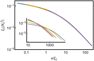
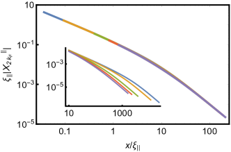
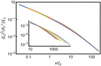
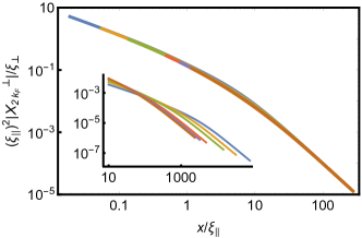
Figure S1: Scaling curves for the four components of the Kondo cloud computed at fixed $\alpha=0.3$ ($J_{\parallel}=2.84$). Raw data is shown in the insets, with different curves correspond to five different values of $\Delta$ collected in the interval $\Delta\in[0.005/a,0.07/a]$ (i.e. $J_{\perp}\in[0.0157,0.220]$).

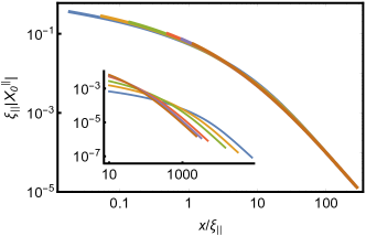
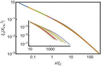
Figure S2: Scaling curves for the four components of the Kondo cloud computed at fixed $\alpha=0.45$ ($J_{\parallel}=2.07$). Raw data is shown in the insets, with different curves correspond to six different values of $\Delta$ collected in the interval $\Delta\in[0.01/a,0.125/a]$ (i.e. $J_{\perp}\in[0.0314,0.393]$).

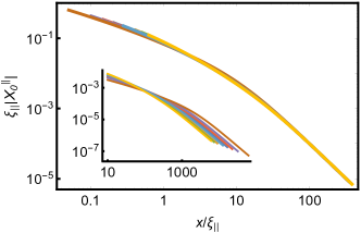
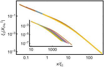
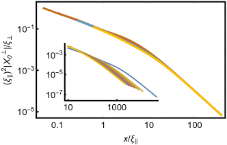
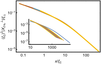
Figure S3: Scaling curves for the four component of the Kondo cloud computed at fixed $\alpha=0.8$ ($J_{\parallel}=0.663$). Raw data is shown in the insets, with different curves correspond to eight different values of $\Delta$ collected in the interval $\Delta\in[0.12/a,0.28/a]$ (i.e. $J_{\perp}\in[0.377,0.880]$).