Prospects for detecting decreasing exoplanet frequency with main sequence age using PLATO

Abstract

The space mission PLATO will usher in a new era of exoplanetary science by expanding our current inventory of transiting systems and constraining host star ages, which are currently highly uncertain. This capability might allow PLATO to detect changes in planetary system architecture with time, particularly because planetary scattering due to Lagrange instability may be triggered long after the system was formed. Here, we utilize previously published instability timescale prescriptions to determine PLATO’s capability to detect a trend of decreasing planet frequency with age for systems with equal-mass planets. For two-planet systems, our results demonstrate that PLATO may detect a trend for planet masses which are at least as massive as super-Earths. For systems with three or more planets, we link their initial compactness to potentially detectable frequency trends in order to aid future investigations when these populations will be better characterized.

1 Introduction

Nearly all exoplanets orbit stars whose ages are poorly constrained. This situation is unfortunate because the potential to learn about the dynamical evolution of planetary systems through the host star’s evolution has yet to be realized. Accurate stellar ages may provide key constraints and insights on the formation and fate of planets.

Tidally-influenced, hot exoplanets highlight the importance of this link. Hundreds of confirmed planets have orbital periods less than 10 days, where tidal interactions between the planet and star can affect the planet’s orbital parameters in a myriad of ways (e.g. see Fig. 4 of Ogilvie, 2014). Because the timescales for shrinking an orbit are sensitively dependent on the orbital period, accurate stellar ages would crucially constrain the dynamical histories of these systems. Further, the details of tidal theory are controversial and recent analyses (e.g. Efroimsky & Makarov, 2013) demonstrate the dangers of adopting the heretofore widely-used constant quality factor. Adding stellar age to the list of known system parameters would enable greater resolution on this topic.

However, the insights obtained from accurate stellar ages are not restricted to substellar companions with such close orbits. Single planets or brown dwarfs which are out of the reach of stellar tides (with semimajor axes beyond about 0.1 au) but within the ellipsoid of the gravitational influence of the parent star within the Milky Way (within about $10^{5}$ au) could attain currently-observed orbital properties from (i) a relic planet formation process such as core accretion, gravitational instability or disc migration (see Baruteau et al., 2013; Helled et al., 2013, for recent reviews), (ii) a relic star formation process such as star-planet scattering in birth clusters (Pfahl & Muterspaugh, 2006; Spurzem et al., 2009; Malmberg et al., 2011; Parker & Quanz, 2012; Hao et al., 2013), (iii) gravitational interaction with other planets during a star’s main sequence lifetime (see Davies et al., 2014, for a recent review) or/and (iv) perturbations from Galactic field star flybys (Zakamska & Tremaine, 2004; Fregeau et al., 2006; Boley et al., 2012; Veras & Moeckel, 2012) and Galactic tides (Heisler & Tremaine, 1986; Brasser, 2001; Veras & Evans, 2013).

All these processes are time-dependent and hence could benefit from accurate stellar ages. Techniques are being developed to constrain stellar ages (Lebreton & Goupil, 2014) to within 10 per cent of a typical main sequence lifetime of a Solar-mass star by utilizing astroseismology. Although these techniques can be applied to high-precision photometric data taken from the CoRoT (Baglin et al., 2002) and Kepler (Borucki et al., 2010; Koch et al., 2010) space missions, the number of suitable stars from these missions is just a handful.

The PLATO space mission (Rauer et al., 2014), due for launch in 2024, will achieve similarly tight age constraints, but for a much larger sample of stars. One of the main aims of PLATO is to achieve 10% precision in the age of 20,000 main sequence stars of spectral types F5-K7. In order to achieve this goal, PLATO will produce internal stellar mass distributions for different stars by combining radius measurements derived from Gaia data with the oscillation frequencies observed in the PLATO light curves.

Other techniques which will be used to derive stellar ages, such as gyrochronology, will be assessed and calibrated from this “primary” sample and then applied to the hundreds of thousands of main sequence stars that PLATO will observe during the course of its 6 year mission (albeit at a lower age precision). Moreover, PLATO will, for the primary sample, allow for direct testing of stellar evolution tracks.

Such a large sample will enable us to detect trends in exoplanetary science that remain currently hidden in the noise. One of these trends is frequency of planets versus main sequence age. Not all systems with multiple planets will remain stable over their main sequence lifetimes. In our own Solar system, Mercury has a one to few per cent chance of destabilizing the inner planets (Laskar & Gastineau, 2009; Zeebe, 2015). Other systems are closer to instability; Section 6.3 of Veras et al. (2013) discuss specific examples for planets discovered by Doppler radial velocity with semimajor axes that exceed 1 au. Overall, the frequency of planets might decrease with time.

The trend for planets detected by transit photometry within 1 au but beyond the limit at which tidal forces cease to become significant (at about 0.1 au) should not be qualitatively different. On 9 Jul 2015, the Exoplanets Data Explorer (http://exoplanets.org) listed 509 substellar objects in this semimajor axis range that are components of multiple-planet systems. Overall, Fang & Margot (2012) and Ballard & Johnson (2014) both estimate that about half of Kepler systems are multiple-planet systems, the latter considering only M dwarfs. Seven examples of potential planets in multi-planet systems are the seven candidate planets of KIC 11442793, all of which transit between 0.074 au and 1.0 au but do not have measured masses (Cabrera et al., 2014). In fact, those authors conclude that the two outermost candidates are indeed planets due to dynamical stability constraints on their masses, highlighting how close to instability some of these systems might reside.

In this brief paper, we combine stability prescriptions from previous investigations with the detection capabilities of the PLATO mission. Section 2 identifies these prescriptions and Section 3 performs the analysis. We conclude in Section 4.

2 Stability of planetary systems

Two-planet systems represent a robust starting point with which to study decreasing planet frequency with time along the main sequence. Observers have identified hundreds of these systems, and theorists have established analytical constraints which would otherwise be unattainable with additional planets.

2.1 Two-planet stability

A two-planet system is a generally-unsolvable three-body problem. However, Marchal & Saari (1975) and Marchal & Bozis (1982) identified allowable regions of motion in this problem based on the angular momentum and energy of the system. This categorization proved particularly valuable after the confident discovery of extrasolar planets (Wolszczan & Frail, 1992) for assessing their stability. Many subsequent studies, summarized in Georgakarakos (2008), considered relevant special cases and extensions.

The allowable regions of motions are partially partitioned by the concept of Hill stability. Two planets are said to be Hill stable if their orbits never cross. This requirement does not preclude the inner planet from crashing into the star, nor the outer planet from escaping from the system. If the planets do remain ordered and do not suffer a collision nor ejection, then the system is said to be Lagrange stable. In Hill unstable cases, when the initial orbits do cross, then the outcome is uncertain: the system could destabilize or alternatively the planets might remain inside of a mean motion resonance (like Neptune and Pluto). This latter possibility presupposes the planets were originally captured into a resonance, most likely due to protoplanetary disc dissipation, but not necessarily (Raymond et al., 2008).

Nevertheless, in most cases (as a fraction of available parameter space), planets which cross orbits will become violently unstable. In this respect, the critical separation $\Delta_{\rm H}$ of the initial planetary orbits that determines the Hill stability boundary has occasionally been treated, erroneously, as a type of global stability boundary. Marzari (2014) has demonstrated why Hill stability should not be treated as a global boundary through a frequency map analysis. In some cases though, the Hill stability boundary may be considered a dividing line between “quick instability” and “slow instability”. This notion may be carried further: one can then define a Lagrange stability boundary $\Delta_{\rm L}>\Delta_{\rm H}$ beyond which Lagrange instability does not occur, or occurs on a timescale which exceeds the main sequence stellar lifetime.

The lack of quantification in these statements results from a dearth of dedicated studies of Lagrange instability. We summarize previous investigations as follows: Chapter 11 of Marchal (1990), Anosova (1996) and Li et al. (2009) focused on the escape of the outer body; Kholshevnikov & Kuznetsov (2011) considered the mass dependence; Deck et al. (2013) linked Lagrange instability (albeit defined slightly differently) with mean motion resonance overlap; and Barnes & Greenberg (2006, 2007), Raymond et al. (2009), Kopparapu & Barnes (2010), Veras et al. (2013) and Veras & Mustill (2013) evaluated the extent of Lagrange instability beyond the Hill stability limit. Recently Petrovich (2015) unveiled a fairly general Lagrange instability criterion for two unequal-mass, highly eccentric and nearly coplanar planets that performs significantly better than previous widely-used criteria from stellar dynamics (Eggleton & Kiseleva, 1995; Mardling & Aarseth, 2001). Although excellent analytic approximations to $\Delta_{\rm H}$ exist (Donnison, 2011), the same is not true for $\Delta_{\rm L}$. One must find $\Delta_{\rm L}$ empirically through simulations. However, simulations have revealed that this Lagrange stability boundary is nebulous.

Veras & Mustill (2013) found that although $\Delta_{\rm L}$ is difficult to constrain, the minimum time to Lagrange instability is well-established empirically as a function of planet mass only, for equal-mass planets. They defined the Lagrange instability timescale as the time at which either the inner planet collided with the stellar surface or when the outer planet’s orbit became hyperbolic. If $x_{\rm uns}$ represents the minimum number of initial orbits of the inner planet before the onset of Lagrange instability, then

$$\log_{10}{\left(x_{\rm uns}\right)}\sim\left(5.23\pm 0.04\right)\left(\frac{\mu}{M_{\rm J}/M_{\odot}}\right)^{-0.181\pm 0.003},$$ (1)

where $\mu$ is the planet/star mass ratio, for both planets, and $M_{\rm J}$ is the mass of Jupiter. This formula appears to hold true for any separation in-between $\Delta_{\rm H}$ and $\Delta_{\rm L}$, for, at least, orbits with initial eccentricities less than 0.3, and is valid for both planets and brown dwarfs. The equation is based on a fit down to masses of $0.1M_{\rm J}$, and will be used directly in conjunction with PLATO sensitivities in Section 3.

2.2 Stability of three or more planets

In systems with three or more planets, there is no known analytical constraint on Hill stability, and the distinction between Hill instability and Lagrange instability is rarely asserted. Instead, researchers have relied on empirical fits to $N$-body simulations to help characterize the potential future stability of a system. Analytical motivation for establishing these fits is also rare. For an exception, see Section 3 of Zhou et al. (2007), who demonstrate how an analytical treatment from first principles can reproduce the same scalings obtained from their empirical fits.

The functional form predominately chosen for the global instability fit for three or more planets is equivalent to (Chambers et al., 1996; Smith & Lissauer, 2009; Funk et al., 2010; Pu & Wu, 2015)

$$\log_{10}\left({x_{\rm uns}}\right)\sim b\beta+c,$$ (2)

although slight variations exist (Faber & Quillen, 2007; Zhou et al., 2007; Chatterjee et al., 2008; Quillen, 2011; Mustill et al., 2014). In equation (2), $b$ and $c$ are fitted constants and $\beta$ refers to the number of mutual Hill radii by which consecutive pairs of planets are separated. A mutual Hill radius is a distance that is not defined uniformly throughout the literature (contrast, e.g., Chambers et al. 1996 and Marzari & Weidenschilling 2002 with Smith & Lissauer 2009, and see the discussion at the end of Section 2 of Mustill et al. 2014). Regardless, effectively, $\beta$ determines the extent of packing in a planetary system (Barnes & Raymond, 2004; Barnes et al., 2008; Raymond et al., 2009; Veras & Gänsicke, 2015), and can be expressed through masses and semimajor axes. Although the exact definition of $\beta$ varies (see also the sentence containing equation 5 in Pu & Wu, 2015), overall if $\beta$ is too small, then the system will become unstable almost immediately. Alternatively, if $\beta$ is too large, the system will not experience instability during the star’s main sequence lifetime.

Like Equation (1), Equation (2) is applicable only for equal-mass planets. However, Equation (2) is more versatile, having been applied to systems with for example 3, 5, 10 and even 20 planets. The unequal-planet mass case greatly increases the available phase space to explore, and has so-far largely been ignored (we do so here as well). Although Equation (2) may be more versatile, this general form does not appear to constrain stability as well as Equation (1), because the latter is for the specific case of two equal-mass planets.

Whereas $\beta$ typically represents a variable user-defined proxy for initial separations, the values of $b$ and $c$ are considered to be fixed and are computed only after a suite of $N$-body simulations has finished running. Both the number of planets as well as the planet mass / star mass ratio under the assumption of initially circular orbits sets both $b$ and $c$; these values might also be weakly dependent on $a_{1}$ and on $\beta$. In fact, the LHS of Equation (2) is more often expressed as an unscaled time.

The wide applicability of Equation (2) for systems with at least three planets is useful for our purposes. Although that equation does not let us directly relate PLATO sensitivities with planetary mass, as in the two-planet case, the relation provides an indirect pathway to do so depending on the architecture a reader might consider.

3 Link with PLATO

Assume that PLATO will be able to constrain a star’s age to $\Delta t_{\rm PLATO}$, such that PLATO will be able to distinguish $(t_{\rm MS}/\Delta t_{\rm PLATO})$ time bins over a star’s main sequence lifetime $t_{\rm MS}$. At the level of approximation we are aiming for, we need not require that the number of time bins is an integer, and may also treat $\Delta t_{\rm PLATO}$ as constant in time. With these assumptions, we can then write the number of initial inner planetary orbits whose total duration encompasses one time bin as

$$x_{\rm min}\equiv\frac{\sqrt{GM_{\star}}\Delta t_{\rm PLATO}}{2\pi a_{1}^{3/2}}.$$ (3)

One can consider $x_{\rm min}$ to be the minimum number of orbits needed to resolve a trend of planet frequency with stellar age.

However, no resolution is possible if the planets (i) fail to become unstable, or (ii) all become unstable too early. In the first case, instability must occur before the start of the last time bin, such that we require

$$x_{\rm uns}<\left(\frac{t_{\rm MS}}{\Delta t_{\rm PLATO}}-1\right)x_{\rm min}.$$ (4)

This condition alone may be sufficient to detect a trend of decreasing planet mass with stellar age. If, however, the instability occurs almost exclusively within the first time bin, then equation (4) is not restrictive enough. In this case, we should also impose the condition

$$x_{\rm uns}>x_{\rm min}.$$ (5)

We choose to leave $\Delta t_{\rm PLATO}$ as an independent variable to allow for the possibility of variations in the stellar constraints on a star-by-star basis. Further, we consider 9 different main sequence stellar masses ($0.7,0.8,0.9,1.0,1.1,1.2,1.3,1.4,1.5M_{\odot}$), corresponding to the range in which asteroseismology with PLATO can be effective at constraining stellar ages. Because we are interested only in Lagrange instability on the main sequence , we must compute the main sequence lifetime $t_{\rm MS}$ of these stars. To do so, we use the sse code (Hurley et al., 2000), and assume Solar metallicity. We obtain $t_{\rm MS}=10948,7646,5607,4237,3355,$ and 2716 Myr for $M_{\star}=1.0,1.1,1.2,1.3,1.4,1.5M_{\odot}$, respectively. The lower mass stars are on the main sequence for a duration greater than the current age of the Universe. Consequently, for added clarity, we do not draw curves in the figures of this paper for the $0.8M_{\odot}$ and $0.9M_{\odot}$ tracks, as they are so similar to the $0.7M_{\odot}$ track.

3.1 Two-planet systems

First consider equation (4) in the context of two-planet systems. Combining that with equation (1) yields the following specific condition on the planet/star mass ratio as a function of $\Delta t_{\rm PLATO}$

$$\frac{\mu}{M_{J}/M_{\odot}}\gtrsim 0.026\bigg{[}1+0.10\log_{10}{}\bigg{\{}$$

$$\ \ \ \ \ \ \ \ \ \ \ \ \ \left(\frac{M_{\star}}{M_{\odot}}\right)^{\frac{1}{2}}\left(\frac{a_{1}}{0.2\ {\rm au}}\right)^{-\frac{3}{2}}\left(\frac{\Delta t_{\rm PLATO}}{1\ {\rm Gyr}}\right)$$

$$\ \ \ \ \ \ \ \ \ \ \ \ \ \times\left(\frac{t_{\rm MS}}{\Delta t_{\rm PLATO}}-1\right)\bigg{\}}\bigg{]}^{-5.55}.$$

(6)

Figure 1: The minimum planet-star mass ratio $\mu$ for which PLATO can detect a decreasing trend of planet frequency versus time for packed, Hill-stable two-planet systems. The $x$-axis refers to the (variable) magnitude of the stellar age constraints PLATO may provide. In the lower panel, the first time bin is excluded, emphasizing its importance at detecting potential trends (shaded regions only). If ages are constrained to within 1 Gyr, then a trend should be detectable for planets at least as massive as $10^{-2}M_{\rm J}$.

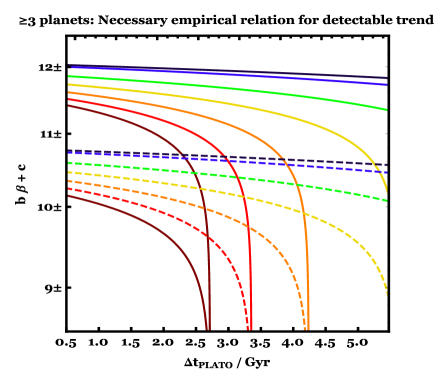
Figure 2: Values of the empirical planet instability relation $(b\beta+c)$ for systems with at least three planets for which PLATO will detect a decreasing trend of planet frequency versus time. The solid and dashed lines coloured lines in the upper panel have the same designations as those in the upper panel of Figure 1. In the lower panel, the first time bin is excluded, such that a detectable trend is possible only in the shaded regions. The $\pm$ symbols in the $y$-axis labels indicate that the demarcated regions may be smeared out in an unpredictable fashion. If the packing parameter $\beta$ is too great, then the systems will not produce a detectable trend.

The upper panel of Figure 1 illustrates the minimum planet masses for which PLATO will be able to detect a trend of decreasing planet frequency with main sequence age, provided that PLATO can discover enough planets at these given masses to build up a large-enough sample. From the PLATO primary sample of stars, we expect many thousands of terrestrial planets with orbital periods up to about one year to be detectable. For a significant proportion of these planets, stellar activity signals will complicate the determination of their masses. However, by just crudely binning observations, PLATO will be able to recover many of these systems. Disentangling stellar activity signals is an ongoing area of research (e.g. Bastien et al., 2014) that will, no doubt, further improve the situation over the next decade.

The first time bin is particularly important, and will contain a large sample of instabilities with which to compare. Consider the consequences of excluding that time bin; the lower panel of Figure 1 also imposes the restriction of Equation (5). If PLATO were to look for trends of planet frequency with stellar age only between the first and last time bins, then the planet mass range for which this technique would be successful is less than an order of magnitude.

In any case, if we assume that PLATO will constrain stellar ages to within 10 per cent for stars of spectral type K7 or earlier, then we can obtain some broad estimates for the planet masses for which a decreasing frequency would be detectable. Consider our model stars for which $M_{\star}\geq 1.0M_{\odot}$. Their values of $t_{\rm MS}$ imply $\Delta t_{\rm PLATO}\lesssim 1$ Gyr always. Therefore, in the equal-mass case (upper panel), PLATO should be able to detect a decreasing frequency trend for planet masses $\sim 10^{-2}M_{\rm J}$ and larger. This statement is also true for $0.7M_{\odot}\leq M_{\star}<1.0M_{\odot}$ because of the flatness of the lowest-mass curve. The bottom panel of Figure 1 also suggests that the trend is detectable for planet masses as low as those found in super-Earths. PLATO will be able to detect these bodies, as well as even sub-Earth planetary radii, and thereby improve our understanding of the currently poorly-constrained radius and mass distributions of the lowest mass planets. Determining masses for the lightest planets is difficult. Recent studies, e.g. Wu & Lithwick (2013) and Weiss & Marcy (2014), have shown potentially tantalising correlations but remain somewhat controversial due to the lack of directly-measured planetary masses.

3.2 Systems with three or more planets

For more complex systems with higher numbers of planets, we cannot make as direct a link with planetary mass as in the two-planet case. Instead, the key constraint is on the quantity $(b\beta+c)$. By using equation (4) we obtain

$$b\beta+c<10.05+\log_{10}{}\bigg{\{}\left(\frac{M_{\star}}{M_{\odot}}\right)^{\frac{1}{2}}\left(\frac{a_{1}}{0.2\ {\rm au}}\right)^{-\frac{3}{2}}\left(\frac{\Delta t_{\rm PLATO}}{1\ {\rm Gyr}}\right)$$

$$\ \ \ \ \ \ \ \ \ \ \ \ \ \ \ \ \ \ \ \ \ \ \ \ \times\left(\frac{t_{\rm MS}}{\Delta t_{\rm PLATO}}-1\right)\bigg{\}}.$$ (7)

We emphasize that the applicability of Equation (7) is limited. The intrinsic scatter in system stability causes so-far-unpredictable deviations from this formula. For example, Fig. 2 of Smith & Lissauer (2009) indicates that for a given set of $(b,c)$, unstable systems can occur for different values of $\beta$ which vary by more than unity.

We plot the curves resulting from Equation (7) in the upper panel of Fig. 2. The $y$-axes labels deliberately contain the symbol $\pm$ in order to indicate the uncertainty described in the last paragraph. Equation (7) implies that if the system is too widely separated initially (with $\beta$ too large), then the instability will never occur quickly enough for a trend to be detectable. Alternatively, $\beta$ can never be too small, because the resulting quick instabilities will be included in the first time bin.

If we exclude this time bin, then the result is the bottom panel of Fig. 2. In this panel, the quantity $(b\beta+c)$ is restricted to just about a few; too small of a range to even encompass the different fits from multiple authors to instability timescales in a similar region of parameter space (see Fig. 3 of Pu & Wu, 2015).

Nevertheless, and despite large phase space of systems with three or more planets, we can make some concrete statements. Consider the study of Smith & Lissauer (2009), whose equation 6 is in the same form as our Equation (2) and who derive sets of $(b,c)$ based on extensive suites of $N$-body numerical integrations. They found that for 5-planet systems where $\mu=3.0035\times 10^{-6}$ (corresponding to Earth-mass planets orbiting a Solar-mass star), $(b,c)=(1.012,-1.686)$ holds for $3.4\lesssim\beta\lesssim 8.4$. These values correspond to $(b\beta+c)\approx\left\{1.8,6.8\right\}$, lower than the ranges presented in Fig. 2. Consequently, instabilities produced from that setup would occur within the first time bin.

Smith & Lissauer (2009) also considered many other system types; for systems with three Earth-mass planets, they fit values of $(b,c)=(1.496,-3.142)$ for $\beta\geq 3.0$, which would give $(b\beta+c)\approx\left\{10,11,12\right\}$ for $\beta\approx\left\{8.78,9.45,10.12\right\}$. These values of $\beta$ would place the systems in other time bins (besides the first). Comparing their 5-planet and 3-planet fits in their fig. 1 reveals that the functional form of the fit might change for $\beta\gtrsim 8.5$. Quantifying how, even for just the equal-mass case, is difficult because of computational limitations. Using $N$-body simulations to predict the very long term ($\sim$Gyrs) evolution of transiting planets (such as those which will be discovered by PLATO) pose an additional challenge because their semimajor axes would be on the scale of hundredths or tenths of an au (whereas Smith & Lissauer 2009 adopted $a_{1}=1$ au).

4 Summary

Compared to previous experiments, the PLATO space mission will significantly improve robust stellar age estimates by developing separate internal mass distributions for thousands of individual stars. Consequently, PLATO will unveil currently undetectable trends in planetary systems. In this work, we demonstrated one such potential trend: decreasing planetary frequency with main sequence age for marginally unstable equal-mass multi-planet systems. For two-planet systems, this trend could be most secure for planetary masses which are on the order of ten Earth masses, well within PLATO’s planet detection capabilities. Detection of this trend could also help constrain formation mechanisms and test the theory (Pu & Wu, 2015; Volk & Gladman, 2015) that tightly packed inner planets were more prevalent in the initial stages of the lifetime of planetary systems.

References

- Anosova (1996) Anosova, J. 1996, AP&SS, 238, 223
- Baglin et al. (2002) Baglin, A., Auvergne, M., Barge, P., et al. 2002, Stellar Structure and Habitable Planet Finding, 485, 17
- Ballard & Johnson (2014) Ballard, S., & Johnson, J. A. 2014, Submitted to ApJ, arXiv:1410.4192
- Barnes & Raymond (2004) Barnes, R., & Raymond, S. N. 2004, ApJ, 617, 569
- Barnes & Greenberg (2006) Barnes, R., & Greenberg, R. 2006, ApJL, 647, L163
- Barnes & Greenberg (2007) Barnes, R., & Greenberg, R. 2007, ApJL, 665, L67
- Barnes et al. (2008) Barnes, R., Goździewski, K., & Raymond, S. N. 2008, ApJL, 680, L57
- Baruteau et al. (2013) Baruteau, C., Crida, A., Paardekooper, S.-J., et al. 2013, arXiv:1312.4293
- Bastien et al. (2014) Bastien, F. A., Stassun, K. G., Pepper, J., et al. 2014, AJ, 147, 29
- Boley et al. (2012) Boley, A. C., Payne, M. J., & Ford, E. B. 2012, ApJ, 754, 57
- Borucki et al. (2010) Borucki, W. J., Koch, D., Basri, G., et al. 2010, Science, 327, 977
- Brasser (2001) Brasser, R. 2001, MNRAS, 324, 1109
- Cabrera et al. (2014) Cabrera, J., Csizmadia, S., Lehmann, H., et al. 2014, ApJ, 781, 18
- Chambers et al. (1996) Chambers, J. E., Wetherill, G. W., & Boss, A. P. 1996, Icarus, 119, 261
- Chambers (1999) Chambers, J. E. 1999, MNRAS, 304, 793
- Chatterjee et al. (2008) Chatterjee, S., Ford, E. B., Matsumura, S., & Rasio, F. A. 2008, ApJ, 686, 580
- Davies et al. (2014) Davies, M. B., Adams, F. C., Armitage, P., et al. 2014, Protostars and Planets VI, 787
- Deck et al. (2013) Deck, K. M., Payne, M., & Holman, M. J. 2013, ApJ, 774, 129
- Donnison (2011) Donnison, J. R. 2011, MNRAS, 415, 470
- Efroimsky & Makarov (2013) Efroimsky, M., & Makarov, V. V. 2013, ApJ, 764, 26
- Eggleton & Kiseleva (1995) Eggleton, P., & Kiseleva, L. 1995, ApJ, 455, 640
- Faber & Quillen (2007) Faber, P., & Quillen, A. C. 2007, MNRAS, 382, 1823
- Fang & Margot (2012) Fang, J., & Margot, J.-L. 2012, ApJ, 761, 92
- Fregeau et al. (2006) Fregeau, J. M., Chatterjee, S., & Rasio, F. A. 2006, ApJ, 640, 1086
- Funk et al. (2010) Funk, B., Wuchterl, G., Schwarz, R., Pilat-Lohinger, E., & Eggl, S. 2010, A&A, 516, A82
- Georgakarakos (2008) Georgakarakos, N. 2008, Celestial Mechanics and Dynamical Astronomy, 100, 151
- Hao et al. (2013) Hao, W., Kouwenhoven, M. B. N., & Spurzem, R. 2013, MNRAS, 433, 867
- Heisler & Tremaine (1986) Heisler, J., & Tremaine, S. 1986, Icarus, 65, 13
- Helled et al. (2013) Helled, R., Bodenheimer, P., Podolak, M., et al. 2013, In Press, Protostars and Planets VI, arXiv:1311.1142
- Hurley et al. (2000) Hurley, J. R., Pols, O. R., & Tout, C. A. 2000, MNRAS, 315, 543
- Kholshevnikov & Kuznetsov (2011) Kholshevnikov, K. V., & Kuznetsov, E. D. 2011, Celestial Mechanics and Dynamical Astronomy, 109, 201
- Koch et al. (2010) Koch, D. G., Borucki, W. J., Basri, G., et al. 2010, ApJL, 713, L79
- Kopparapu & Barnes (2010) Kopparapu, R. K., & Barnes, R. 2010, ApJ, 716, 1336
- Koriski & Zucker (2011) Koriski, S., & Zucker, S. 2011, ApJL, 741, LL23
- Laskar & Gastineau (2009) Laskar, J., & Gastineau, M. 2009, Nature, 459, 817
- Lebreton & Goupil (2014) Lebreton, Y., & Goupil, M. J. 2014, A&A, 569, A21
- Li et al. (2009) Li, P. J., Fu, Y. N., & Sun, Y. S. 2009, A&A, 504, 277
- Lissauer et al. (2011) Lissauer, J. J., Fabrycky, D. C., Ford, E. B., et al. 2011, Nature, 470, 53
- Lissauer et al. (2013) Lissauer, J. J., Jontof-Hutter, D., Rowe, J. F., et al. 2013, ApJ, 770, 131
- Malmberg et al. (2011) Malmberg, D., Davies, M. B., & Heggie, D. C. 2011, MNRAS, 411, 859
- Marchal (1990) Marchal, C. 1990, Studies in Astronautics, Studies in Aeronautics, 4. Amsterdam: Elsevier, 1990
- Marchal & Saari (1975) Marchal, C., & Saari, D. G. 1975, Celestial Mechanics, 12, 115
- Marchal & Bozis (1982) Marchal, C., & Bozis, G. 1982, Celestial Mechanics, 26, 311
- Mardling & Aarseth (2001) Mardling, R. A., & Aarseth, S. J. 2001, MNRAS, 321, 398
- Marois et al. (2010) Marois, C., Zuckerman, B., Konopacky, Q. M., Macintosh, B., & Barman, T. 2010, Nature, 468, 1080
- Marzari & Weidenschilling (2002) Marzari, F., & Weidenschilling, S. J. 2002, Icarus, 156, 570
- Marzari (2014) Marzari, F. 2014, MNRAS, 442, 1110
- Masuda (2014) Masuda, K. 2014, ApJ, 783, 53
- Mustill & Villaver (2012) Mustill, A. J., & Villaver, E. 2012, ApJ, 761, 121
- Mustill et al. (2014) Mustill, A. J., Veras, D., & Villaver, E. 2014, MNRAS, 437, 1404
- Nordhaus & Spiegel (2013) Nordhaus, J., & Spiegel, D. S. 2013, MNRAS, 432, 500
- Ogilvie (2014) Ogilvie, G. I. 2014, ARA&A, 52, 171
- Parker & Quanz (2012) Parker, R. J., & Quanz, S. P. 2012, MNRAS, 419, 2448
- Pearce & Wyatt (2014) Pearce, T. D., & Wyatt, M. C. 2014, MNRAS, 443, 2541
- Petrovich (2015) Petrovich, C. 2015, ApJ, In Press, arXiv:1506.05464
- Pfahl & Muterspaugh (2006) Pfahl, E., & Muterspaugh, M. 2006, ApJ, 652, 1694
- Pu & Wu (2015) Pu, B., & Wu, Y. 2015, In Press, ApJ, arXiv:1502.05449
- Quillen (2011) Quillen, A. C. 2011, MNRAS, 418, 1043
- Rauer et al. (2014) Rauer, H., Catala, C., Aerts, C., et al. 2014, Experimental Astronomy, 41
- Raymond et al. (2008) Raymond, S. N., Barnes, R., Armitage, P. J., & Gorelick, N. 2008, ApJL, 687, L107
- Raymond et al. (2009) Raymond, S. N., Barnes, R., Veras, D., et al. 2009, ApJL, 696, L98
- Smith & Lissauer (2009) Smith, A. W., & Lissauer, J. J. 2009, Icarus, 201, 381
- Spurzem et al. (2009) Spurzem, R., Giersz, M., Heggie, D. C., & Lin, D. N. C. 2009, ApJ, 697, 458
- Swift et al. (2013) Swift, J. J., Johnson, J. A., Morton, T. D., et al. 2013, ApJ, 764, 105
- Veras & Evans (2013) Veras, D., & Evans, N. W. 2013, MNRAS, 430, 403
- Veras & Moeckel (2012) Veras, D., & Moeckel, N. 2012, MNRAS, 425, 680
- Veras et al. (2013) Veras, D., Mustill, A. J., Bonsor, A., & Wyatt, M. C. 2013, MNRAS, 431, 1686
- Veras & Mustill (2013) Veras, D., & Mustill, A. J. 2013, MNRAS, 434, L11
- Veras & Gänsicke (2015) Veras, D., Gänsicke, B. T. 2015, MNRAS, 447, 1049
- Villaver et al. (2014) Villaver, E., Livio, M., Mustill, A. J., & Siess, L. 2014, ApJ, 794, 3
- Volk & Gladman (2015) Volk, K., & Gladman, B. 2015, ApJL, 806, L26
- Weiss & Marcy (2014) Weiss, L. M., & Marcy, G. W. 2014, ApJL, 783, LL6
- Wolszczan & Frail (1992) Wolszczan, A., & Frail, D. A. 1992, Nature, 355, 145
- Wolszczan (1994) Wolszczan, A. 1994, Science, 264, 538
- Wu & Lithwick (2013) Wu, Y., & Lithwick, Y. 2013, ApJ, 772, 74
- Zakamska & Tremaine (2004) Zakamska, N. L., & Tremaine, S. 2004, AJ, 128, 869
- Zeebe (2015) Zeebe, R. E. 2015, ApJ, 798, 8
- Zhou et al. (2007) Zhou, J.-L., Lin, D. N. C., & Sun, Y.-S. 2007, ApJ, 666, 423