Zentrum für Mathematische Physik, Universität Hamburg, Bundesstrasse 55, 20146 Hamburg, Germany bbinstitutetext: Institute for Theoretical Physics and Spinoza Institute, Utrecht University,
Leuvenlaan 4, 3584 CE Utrecht, The Netherlandsccinstitutetext: Hamilton Mathematics Institute and School of Mathematics,
Trinity College, Dublin 2, Ireland
Puzzles of -deformed
Abstract
We derive the part of the Lagrangian for the sigma model on the -deformed space which is quadratic in fermions and has the full dependence on bosons. We then show that there exists a field redefinition which brings the corresponding Lagrangian to the standard form of type IIB Green-Schwarz superstring. Reading off the corresponding RR couplings, we observe that they fail to satisfy the supergravity equations of motion, despite the presence of -symmetry. However, in a special scaling limit our solution reproduces the supergravity background found by Maldacena and Russo. Further, using the fermionic Lagrangian, we compute a number of new matrix elements of the tree level world-sheet scattering matrix. We then show that after a unitary transformation on the basis of two-particle states which is not one-particle factorisable, the corresponding T-matrix factorises into two equivalent parts. Each part satisfies the classical Yang-Baxter equation and coincides with the large tension limit of the -deformed S-matrix.
ITP-UU-15-10
TCD-MATH-15-05
ZMP-HH-15-19
1 Introduction and summary
In many instances a better understanding of a physical system or theory takes place once this system or theory is put under deformation. Recently there was an interesting proposal on how to deform the sigma model for strings on while keeping its classical integrability Delduc:2013qra . Deformations of this type constitute a general class of the so-called Yang-Baxter deformations Klimcik:2002zj ; Klimcik:2008eq , which in modern parlance comprise - Delduc:2013qra , Arutyunov:2013ega -Engelund:2014pla and -deformations Sfetsos:2013wia -Demulder:2015lva , as well as deformations related to solutions of the classical Yang-Baxter equation Kawaguchi:2014qwa -vanTongeren:2015uha . Our primary interest in studying these deformations is that they typically break (super)symmetries of the original string model, yet allowing for a possibility to solve them exactly.
Here we continue the studies of the -deformed sigma model based on a solution of the modified classical Yang-Baxter equation corresponding to the standard Dynkin diagram of the superalgebra. Recall that for this model the metric and the -field are explicitly known Arutyunov:2013ega . At the classical level the model exhibits a local fermionic -symmetry and a hidden symmetry Delduc:2014kha . It was shown Arutyunov:2013ega that its world-sheet bosonic tree-level scattering matrix factorises into two copies, each of which coincides under proper identification of the parameters with the large tension limit of the -deformed S-matrix found from quantum group symmetries, unitarity and crossing Beisert:2008tw ; Hoare:2011wr .
The aim of the present paper is to clarify an important question of whether or not the -deformed model is type IIB string sigma model. As we will show, under certain assumptions the answer turns out to be negative.
One way to approach this question would be to try to find an embedding of the given NSNS background into a full solution of type IIB supergravity. Given complexity of the NSNS background, this appears however a rather difficult task. First of all the equation for the dilaton has many solutions and also many components of the RR forms seem to be switched on. Surprisingly, -deformations and deformations based on solutions of the classical Yang-Baxter equation behave better in this respect, and some of the metrics could be completed to a full supergravity solution. Even if successful, this approach does not however guarantee that the string sigma model in the corresponding supergravity background will actually coincide with a deformed model.
Another way to proceed is to note that the Green-Schwarz action restricted to quadratic order in fermions contains all the information about the background fields. The corresponding Lagrangian has the form, see e.g. Tseytlin:1996hs ; Cvetic:1999zs ; Wulff:2013kga ,
where are two Majorana-Weyl fermions of the same chirality. The operator acting on fermions has the following expression
where constitute a vielbein, the spin connection and the field strength of a -field, while ’s are RR forms and is a dilaton. Note that the dilaton and RR forms appear only through the combination . An approach we undertake in this paper will be therefore to work out the quadratic fermionic action starting from the -deformed action of Delduc:2013qra and some conveniently chosen representative of the coset . Then we need to find a field redefinition which brings this action into the Green-Schwarz canonical form above. This would allow us to identify the background fields and further check if they satisfy the equations of motion of type IIB supergravity and, in particular, to find a solution for the dilaton. Such a strategy works perfectly, for instance, for the sigma model Metsaev:1998it .
We succeeded in constructing a field redefinition which brings the quadratic fermionic Lagrangian of the -deformed theory to the canonical form. However, reading off the corresponding RR couplings222Throughout the paper we loosely refer to -forms as to RR couplings although as found a posteriori they are not a part of a supergravity background. in section 2.3, we find that they fail to satisfy the supergravity equations! The next surprising observation is that these couplings do not meet the necessary conditions of the mirror duality Arutyunov:2014jfa , and, as the consequence, the mirror background Arutyunov:2014cra is not reproduced in the expected limit . Although this duality is a symmetry of the exact S-matrix, it involves rescaling of the string tension and therefore its absence in the classical Lagrangian might be explained by the order of limits problem.
Another interesting observation, which supports the correctness of our result, concerns a reproduction of a known string background. As was previously noted by one of us SF , there is a special scaling limit under which the -deformed metric and -field reproduce the NSNS part of the Maldacena-Russo background Maldacena:1999mh dual to a non-commutative Yang-Mills theory.333The NSNS part of the Maldacena-Russo background also appears in the context of deformations related to solutions of the classical Yang-Baxter equation Matsumoto:2014gwa . Now we observe that in this limit the RR couplings we found precisely reproduce the rest of the Maldacena-Russo background which is a genuine solution of type IIB supergravity.
In view of these surprising results it is time to ask how our findings are compatible with -symmetry, especially in view of the work Grisaru:1985fv ; Bergshoeff:1985su , where it was shown that the fulfilment of the supergravity constraints is sufficient for the Green-Schwarz action to be invariant under -symmetry. To answer this question, we have explicitly developed the -symmetry transformations of the -deformed model Delduc:2013qra to the leading order in fermions. We then find that the same field redefinition which brings the original Lagrangian to the canonical Green-Schwarz form also brings the -symmetry variations of the target-space coordinates to the standard form in type IIB theory. Then the variation of the world-sheet metric automatically acquires the standard form as well and contains RR couplings, allowing therefore for their independent determination. The RR couplings we read off from the -variations of the world-sheet metric coincide with what we found from the canonical Lagrangian. Clearly, at the level of the quadratic Lagrangian -symmetry cannot say anything about equations of motion for RR couplings. Indeed, the latter couple to fermion bilinears and their leading order -symmetry variations should be combined with variations of the quartic fermionic terms to produce differential constraints on ’s which guarantee invariance of the action. The failure of the RR couplings to satisfy the supergravity equations including the Bianchi identities suggests that -symmetry transformations in the -deformed theory will deviate from that of the Green-Schwarz superstring beyond the leading order.
Now we comment on the issue of field redefinitions. How can one be sure that no other field redefinitions exist which produce better results for RR couplings? Note that we already brought our Lagrangian to the canonical form where NSNS fields appear automatically to be the same as determined from the bosonic action. Thus, if we want to perform further field redefinitions we have to require that they keep the NSNS part of the fermionic action untouched and change exclusively the RR content. Moreover, in the limit such redefinitions should either trivialize or become a symmetry transformation of the undeformed model and the same must be true for the scaling limit to the Maldacena-Russo background. By performing an infinitesimal analysis we then show that there is no smooth -dependent transformation of fields which reduces to the identity in the limit and does not modify the NSNS part of the action. An existence of discrete, i.e. -independent transformations is much more difficult to rule out and, therefore, our result on non-existence of the supergravity background is only applied if no such transformation exists.
Since inclusion of fermions leads to a variety of puzzling results, we find it interesting to extend our earlier computation of the bosonic tree-level two-particle S-matrix Arutyunov:2013ega to include fermions. What we are computing is in fact T-matrix. In the purely bosonic case this T-matrix factorises into two parts, each satisfies the classical Yang-Baxter equation (i.e. it is a classical -matrix) and coincides with the leading term of the large tension expansion of the known -deformed S-matrix. In other words, this T-matrix has precisely the same properties as its undeformed counterpart. We then use our quadratic fermionic Lagrangian to compute new elements in the scattering matrix and discover that this time it does not factorise on two copies. This nice property is spoiled by Boson+Fermion Boson+Fermion scattering elements. However, there exists a unitary momentum-independent transformation of the basis of two-particle states which brings our T-matrix to a factorisable form. Each factor coincides with the large tension limit of the -invariant S-matrix. The transformation of the two-particle basis we found does not however admit a factorisation on transformations of one-particle states. A similar situation has been observed at the one- and two-loop level where integrability of the corresponding S-matrix obtained through unitarity-based methods also required a (momentum-dependent) one-particle-unfactorisable rotation on the basis of two-particle states Engelund:2014pla .444One important difference, though, is that in Engelund:2014pla factorisation of the T-matrix could be also achieved by performing a one-particle transformation which made however the spin and dimension of single-particle states complex. We note that one can think about our unitary transformation as acting on the Hamiltonian which then becomes highly non-local. Moreover, this transformation is -independent and is therefore a symmetry of the undeformed S-matrix.
The light-cone Hamiltonian has an important feature. Although the theory has only -deformed supersymmetry, the masses of bosons and fermions in the light-cone Hamiltonian appear to be the same and they both have a mild dependence of the deformation parameter. Thus, the BMN vacuum is supersymmetric just as it was in the undeformed case.
The paper is organised as follows. In the next section we recall the basic facts about the -deformed sigma model, describe the main steps in the derivation of the fermionic quadratic Lagrangian, present and discuss our main result on the RR couplings. Section 3 contains an alternative derivation of the RR couplings from -symmetry. Section 4 is devoted to the discussion of residual field redefinitions. In section 5 we present the T-matrix and discuss how to achieve its factorisation and fulfilment of the Yang-Baxter equation. Definitions and technical derivations are relegated to three appendices. For the reader’s convenience we also attach appendix D with the equations of motion of type IIB supergravity.
2 Quadratic fermionic Lagrangian and RR couplings
2.1 -deformed model
Let us recall that the Lagrangian density of the -deformed model is given by Delduc:2013qra
| (2.1) |
and the action is normalised as . We use the notations and conventions from Arutyunov:2009ga : ; , ; is the effective string tension. The current , where is a coset representative from . The operators and acting on the currents are defined as
where , , are projections on the corresponding components of the -graded decomposition of the superalgebra , see appendix A.1.
The operator acts on as follows
| (2.2) |
where is a linear operator on which in this paper we define as
| (2.3) |
where is an arbitrary matrix. This choice of corresponds to the standard Dynkin diagram of .
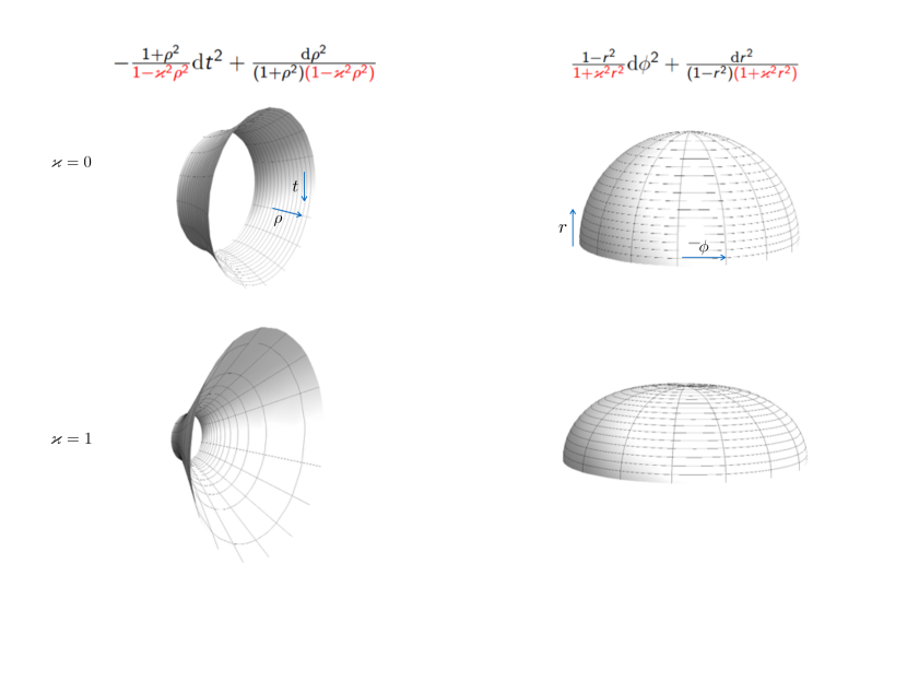
In our previous paper Arutyunov:2013ega the fermions were switched off, a particular choice of the bosonic coset element was made, and the operator was found and used to determine the bosonic part of the -deformed action. Introducing the convenient deformation parameter and , the -deformed metric and the -field can be written in the form
| (2.4) | ||||
| (2.5) | ||||
| (2.6) |
The effect of the deformation on the shape of AdS2 and is shown on Figure 1.
In what follows for convenience we are enumerating the coordinates as
| (2.7) | ||||||||
so that the non-vanishing components of the -field are and while the non-vanishing components of the field strength are and .
To find the part of the -deformed action quadratic in fermions we use the following coset element
| (2.8) |
where the bosonic element is the same as in Arutyunov:2013ega . The element which comprises fermionic degrees of freedom can be defined through the exponential map , or as . The two choices produce the same expression if we stop at quadratic order. The Lie algebra element is a linear combination of odd generators of the algebra555See appendix A.1 for the definition of the generators we use. .
The current can be decomposed in terms of linear combinations of the generators of the algebra
| (2.9) |
It is useful to look at the purely bosonic and purely fermionic currents separately, that are found by switching off fermions and bosons respectively. The purely bosonic current is a combination of even generators and
| (2.10) |
where is the vielbein and is the corresponding spin connection whose explicit expressions can be found in appendix A.4.
The purely fermionic current is decomposed in terms of even and odd generators
| (2.11) |
where we have defined the yet to-be-determined quantities . Expanding in powers of up to quadratic order in fermions we find
| (2.12) | ||||
where and refers to the quantities related to and , respectively, and the matrices are defined in (A.31). The computation of the full current is similar and one gets
where the operator acting on fermions is given by
| (2.14) |
Sometimes it is useful to split this operator as
| (2.15) |
where is the covariant derivative acting on fermions.
The action of the projections and on the current are found from the formulae
| (2.16) |
In particular, the -part of the current is irrelevant for the computation of the Lagrangian, since it is projected out when defining the coset.
The next step consists in constructing the inverse of the operator
| (2.17) |
To this end, we find convenient to expand it in powers of fermions as
| (2.18) |
where is the contribution at order . On generators of degree 0 the inverse operator acts as the identity, at any order in fermions. To find its action on the other generators, we invert it perturbatively in powers of fermions:
| (2.19) |
where is the contribution at order . The leading contribution was already derived in Arutyunov:2013ega . Demanding that we find
| (2.20) | ||||
We will not need higher order contributions. To keep the discussion transparent, for an explicit construction of up to quadratic order in fermions we refer the reader to appendix B.1.
2.2 Quadratic fermionic Lagrangian
Substituting now all the ingredients, that is the current (2.1) and into the Lagrangian (2.1), we expand it up to quadratic order in fermions. At leading order we find the already known Arutyunov:2013ega bosonic Lagrangian
| (2.21) |
where is the vielbein of and the coefficients are presented in appendix B.1, see eqs.(B.12) and (B.13). We can rewrite this result in the standard sigma model form recovering the deformed metric (2.4), (2.5) and the -field (2.6), which happens due to the identities
| (2.22) |
where is a vielbein for the deformed metric which we present in appendix A.4 and is the Minkowski metric (A.28).
In the expansion of the Lagrangian (2.1) in powers of fermions, contributions to a given power come from three sources: from the current , from the operator and from the current . Thus, the quadratic fermionic Lagrangian is a sum of six terms
| (2.23) | ||||
where three numbers in the brackets indicate powers of fermions coming from , and , respectively. For the first two contributions we find
| (2.24) | ||||
where . Note that the sum of gives a non-trivial contribution also to the Wess-Zumino term, since the matrix has a non-vanishing anti-symmetric part.
Concerning the contribution , in appendix B.2 we manipulate the initial result (B.24) to bring it to the form most close to the canonical one
| (2.25) |
which holds up to a total derivative.
Now we spell out the contributions stemming from the inverse operator taken at first order in the expansion. The two contributions can be naturally considered together666The result can be put in this form thanks to the properties (B.7).
| (2.26) | |||||
Finally, the last contribution to the Lagrangian is delivered by the term where the inverse operator is taken at order . We find
| (2.27) | |||||
The last two expressions involve the coefficients which are collected in appendix B.1.
Summing up all the above contributions, we discover that the result is not the standard Green-Schwarz Lagrangian, see the Introduction. Yet, in the undeformed limit it reduces to that one. Indeed, when , the contributions and vanish, while in eq.(2.24) becomes , so that (2.24) transforms into the standard kinetic term, while (2.25) provides its Wess-Zumino completion.777In particular, the self-dual five-form of the background arises from the term with in the definition (2.14) of the operator Metsaev:1998it . This is of course expected because the canonical form of the undeformed Lagrangian is intrinsically built in our construction based on global symmetries and the choice (2.8) of the coset representative. On the other hand in the deformed model the coset plays an auxiliary role because only six commuting isometries remain unbroken. It is thus clear that the Lagrangian we got describes couplings of bosons with fermion bilinears written with a more or less arbitrary choice of coordinates and that field redefinitions will in general modify its form. Our next task is therefore to find a field redefinition that will cast (2.23) in the desired canonical form.
To search for necessary field redefinitions we need a guidance principle. All terms in can be split into two parts: the kinetic part , which contains all couplings of the form , and the mass part , which constitutes the rest of the Lagrangian. The idea is to concentrate just on the kinetic part and find field redefinitions which bring it to the canonical form. In the process new mass terms will be generated and we look at all of them at the very end. Clearly, two types of field redefinitions are possible: rotations of fermions with coefficients depending on bosons and shifts of bosons by fermion bilinears. In the second case, the bosonic Lagrangian will generate contributions to and if we do not want to create higher derivatives of , the corresponding shifts should be of the form
| (2.28) |
with boson-dependent coefficients .
Next, all the terms in are naturally divided according to their symmetry properties into two categories and . Given an expression of the form , we classify it according to
| (2.29) | ||||
The symmetry properties are manifested through purely algebraic manipulations, not by integrating by parts. They are inherited from symmetries of gamma matrices contained in and from the behaviour of under the exchange of . We then show in appendix B.3 that there exists a choice of the coefficients in (2.28) such that the corresponding shift completely removes , leaving behind a bunch of new mass terms. As to , it remains untouched under this shift because the symmetry properties of the derivative couplings generated by (2.28) are opposite to that of . The only manipulations we are left with at this point are boson-dependent rotations of fermions. Since and the canonical kinetic term share the same symmetry (2.29), a rotation which transforms one into the other always exists and we find its explicit form in appendix B.3.
Through the shift of bosons and the rotation of fermions we generated quite a lot of new mass terms. It is now time to sum them up and group together according to their tensorial structures. Quite remarkably, after this is done, the mass part turns out to automatically fit the canonical arrangement. In terms of a -dimensional Majorana fermion of positive chirality (A.54), our Lagrangian is therefore
| (2.30) |
where the operator enjoys the canonical form888The -dimensional -matrices are given in (A.50).
| (2.31) | ||||
In the last equation is the same vielbein of the -deformed metric, c.f. appendix A.4, that features in the bosonic Lagrangian, while is the spin connection that is related to by the standard formula (A.62). Finally, for the 3-form we find the following two non-vanishing components
| (2.32) |
These are precisely the field strength components of the -field (2.6) written with the flat space indices. Thus, we completely restore the NSNS background of the -deformed theory at the level of the quadratic fermionic action, which is rather non-trivial by itself and provides a strong validity check of our computation.
Postponing the discussion of the RR couplings till the next section, we conclude by pointing out that the field redefinitions of we used do not involve world-sheet derivatives and, as such, they can be viewed as a certain -dependent reparametrisation of the original coset representative (2.8) of .
2.3 RR couplings
Here we present our main result – the RR couplings of the -deformed theory, and then discuss some of their features. From eq.(2.31) we find the following non-vanishing RR forms written with flat indices of the tangent space
| (2.33) |
| (2.34) | ||||||
| (2.35) | ||||||
For simplicity we have defined the common coefficient
| (2.36) |
For the five-form we presented here only half of all its non-vanishing components, namely those which involve the index . The other half is obtained from the self-duality equation for the five-form. The answer appears to be rather simple and in the limit all the components vanish except which reduces to the constant five-form flux of the background.
For the reader’s convenience we present the same results written in curved indices
| (2.37) |
| (2.38) | ||||||
| (2.39) | ||||||
Inspection of the found RR couplings reveals that contrary to the natural expectations they do not obey equations of motion of type IIB supergravity.
First of all for the Bianchi identities this is already obvious from the expression (2.37) for the 1-form. To fit the supergravity content this form must be exact , where is axion. One can verify that there is no way to split off an integrating factor in (2.37), such that the corresponding becomes exact.
Concerning other equations of motion, consider, for instance, the Einstein equations (D.12) which involve an unknown dilaton. One can show that to achieve vanishing of the off-diagonal components of the Einstein equations the dilaton must be of the form
| (2.40) |
where and are some functions. However, analysis of the diagonal components of the Einstein equations shows that a solution for and does not exist.
Now we will attempt to make contact of our findings with known supergravity solutions by considering special limits.
Mirror background
We first analyse a special limit . Rescaling the bosonic coordinates of the -deformed metric as
| (2.41) |
and then sending , yields upon an overall rescaling the metric for the mirror model Arutyunov:2014cra . The -field vanishes in this limit. The resulting metric can be then embedded into a full solution of type IIB supergravity by supplementing it with a dilaton and a five-form flux Arutyunov:2014cra .
Now we look at how the actual RR couplings behave in this limit. Upon rescaling (2.41) it is enough to keep only those components with tangent indices that are of order at large to compensate the power coming from the vielbein that multiplies the RR couplings in eq.(2.31). The surviving components are thus
| (2.42) | |||
This result does not match the proposed mirror background Arutyunov:2014cra , and the limiting couplings continue to displease the supergravity equations.
Maldacena-Russo background
Here we look at a special limit and show that the solution we found reproduces in this limit the Maldacena-Russo (MR) background Maldacena:1999mh which is a genuine solution of supergravity equations.
To achieve this limit, we first rescale the coordinates parameterising the deformed AdS space as
| (2.43) |
where is a parameter, and then send . Because the coordinates of the deformed S5 do not undergo any rescaling, the corresponding part of the metric just reduces in this limit to the underformed metric on S5, and the components of the -field in those directions vanish. The AdS part of the metric and the -field remain non-trivial and we find
| (2.44) | ||||
which is precisely the NSNS content of the MR background.
Now we apply the same limiting procedure to the components of the RR couplings (2.33), (2.34) and (2.35) and find that the axion vanishes, and only one component of and one of (plus its dual) survive
| (2.45) |
If we identify the dilaton as
| (2.46) |
where is a constant, we then find that the non-vanishing components for the RR fields, written both with tangent and curved indices, are
| (2.47) | ||||||
These are precisely the dilaton and the RR fields of the MR background Maldacena:1999mh . It is very interesting that despite incompatibility with supergravity equations for generic values of the deformation parameter, there exists a certain limit, different from , where this compatibility is retrieved.
3 RR couplings from -symmetry
As was shown in Delduc:2013qra ; Delduc:2014kha , the Lagrangian of the deformed model is invariant under -symmetry transformations. Recall that in the undeformed case -transformations are implemented by multiplying a group representative of a coset element from the right:
| (3.1) |
where is a local fermionic parameter which takes values in . Here on the right hand side is a new coset representative and is a compensating transformation from . For generic this transformation is not a symmetry of the action, but for a special choice
| (3.2) |
one can show that this is indeed the case Arutyunov:2009ga . The spinors and are local transformation parameters which under -decomposition have degree and , respectively.
In the deformed case one can still prove the existence of a local fermionic symmetry of the form (3.1). However, to achieve the invariance of the action the definition (3.2) has to be modified, in particular will no longer lie just in the odd part of the algebra, but will have a non-trivial overlap with the even part. Precisely, is written in terms of an odd element as Delduc:2013qra
| (3.3) |
where is the operator defined in (2.17) and the two projections are999Comparing to Delduc:2013qra we have dropped the factor of because we use “anti-hermitian” generators.
| (3.4) | ||||
where we defined
| (3.5) |
In appendix B.4 we explicitly derive the variations of bosonic and fermionic fields implied by the above definitions, and observe that they do not have the usual form of the -variations of type IIB superstring. However, after implementing the field redefinitions of appendix B.3, which were needed to put the Lagrangian in the canonical Green-Schwarz form, we find that also the kappa-variations become indeed standard
| (3.6) | ||||
where
| (3.7) |
and is related to as in (B.81). It is now instructive to also look at the kappa-variation for the world-sheet metric, as this provides an independent way to derive the couplings of the fermions to the background fields. The variation is given by Delduc:2013qra
| (3.8) |
where and the projections of a vector are defined as
| (3.9) |
As we show in appendix B.4, after taking into account the field redefinitions performed to get the canonical action, we find a standard kappa-variation also for the world-sheet metric
| (3.10) | ||||
where we have defined
| (3.11) |
The operator turns out to be the same as obtained earlier in the Lagrangian approach. It is given by eq.(2.31), and, in particular, it contains the same RR couplings as found in section 2.3.
We point out that at the level of the quadratic fermionic action, the requirement of -symmetry is unable to produce differential constraints on the RR fields, in particular, the Bianchi identities. Constraints will start to emerge from the quartic action, because to check its invariance, one has to vary the RR couplings entering the quadratic part of the fermionic action, which will lead to the appearance of their derivatives. Thus, if our result for the RR couplings is an ultimate one, i.e. if there are no further field redefinitions changing the RR couplings only, one could expect that at higher orders in fermions both -symmetry transformations and the corresponding Lagrangian start to deviate from the standard form in the theory of IIB Green-Schwarz superstring, and this could explain why our results are compatible with the work Grisaru:1985fv ; Bergshoeff:1985su . It is also worth stressing that in Grisaru:1985fv ; Bergshoeff:1985su it was shown that the supergravity constrains are sufficient for -symmetry of the Green-Schwarz action, whether they are also necessary is unknown to us.
4 On field redefinitions
In the previous section we were able to transform the original Lagrangian into the canonical form and further observed that the RR couplings derived from the latter do not satisfy the supergravity equations. On the other hand, the NSNS couplings in the quadratic fermionic action are properly reproduced and they are the same as found earlier from the bosonic Lagrangian. Therefore we are motivated to ask whether further field redefinitions could be performed which exclusively change the RR content of the theory. It appears to be rather difficult to answer this question in full generality. We will argue however that no field redefinition of this type, continuous in the deformation parameter exists.
We will work in the formulation with 32-dimensional fermions obeying the Majorana and Weyl conditions, see appendix A.3. We start with considering a generic rotation of fermions101010One could imagine more complicated redefinitions like , etc. They were not needed to bring the original Lagrangian to the canonical form and we do not consider them here. These redefinitions will generate higher derivative terms in the action, whose cancellation would imply further stringent constraints on their possible form.
| (4.1) |
where are rotation matrices which depend on bosonic fields. We write as an expansion over a complete basis in the space of -matrices
| (4.2) | ||||
where we have introduced
Next, the coefficients and are -matrices and they can be expanded over the complete basis generated by and identity, see appendix A.3 for the definition and properties of . Further, we require that the transformation preserves chirality and the Majorana condition. Conservation of chirality implies that the -matrices appearing in the expansion of must commute with , i.e. the expansion involves of even rank only
| (4.3) | ||||
In this expansion there are no matrices of higher rank, because those by virtue of duality relations are re-expressed via matrices of lower rank. The Majorana condition imposes the requirement
| (4.4) |
which implies that the coefficients are real. Coefficients of are then given by
| (4.5) |
Thus, the total number of degrees of freedom in the rotation matrix is
which is precisely the dimension of . This correctly reflects the freedom to perform general linear transformations on 32 real fermions of type IIB.
Under these rotations the kinetic part of the fermionic Lagrangian transforms into
| (4.6) | |||
The requirement that under rotations the kinetic part remains unchanged can be formulated as the following conditions on :
| (4.7) | ||||
where “removable terms” means terms which can be removed by shifting bosons in the bosonic action by fermion bilinears. The equations (4.7) should hold on chiral fermions, that is as sandwiched between two chirality projectors. To make the discussion simple, we will not indicate these projectors explicitly till the very end. In the following it is enough to analyse the first equation in (4.7) and, thus, we are led to understand the structure of , which in general has an expansion over a basis of odd rank . The strategy is to determine first the structure of removable terms. To this end we need to study the properties of fermion bilinears.
Suppose that , with . Now we take two sets of Majorana-Weyl fermions, that we call and in order to distinguish them. We consider odd rank -matrices (not to get vanishing expressions)
| (4.8) | ||||
see appendix A.3 for the definition of the numbers . The kinetic term for bosons under the shift, which can be schematically represented as
| (4.9) |
will generate the fermionic terms containing the terms
| (4.10) |
Clearly, for this expression to fit the structure of the fermionic kinetic term, the two terms in the right hand side of (4.10) must be equal. Identifying with and with in eq.(4.8) shows that removable structures in the fermionic action are those for which . Indeed, the structures with entering in the shift (4.9) simply vanish because of the same equation (4.8) considered for . Using the results of appendix A.3 one can determine for various and and the corresponding values are collected in Table 1.
According to this table, the condition that the kinetic term is invariant up to the terms removable by a shift of bosons can be now written as
| (4.11) | ||||
Here -tensors are arbitrary coefficients which parametrise the structures which can be removed from the action by shifting bosons. Obviously, putting a generic satisfying the Majorana-Weyl conditions in the left hand side of (4.11), one would expect an appearance on the right hand side of all these -tensors. But do they actually appear? As we show in a moment the answer is negative.
Combining equations (4.1) and (4.4), we get
| (4.12) |
Now collect all terms on the right hand side of (4.11) that are removable by shifting bosons into a tensor . This tensor has the following symmetry property111111Notice that to exhibit this symmetry property, one has to transpose also the indices , on top of transposition in the space.
| (4.13) |
Note that the tensor in the canonical kinetic term has exactly the opposite symmetry property
| (4.14) |
Putting this information together, let us consider (4.11) written as
| (4.15) |
We take transposition and we multiply by from the left and from the right
| (4.16) |
and further manipulate as
| (4.17) |
With the help of eqs.(4.12) , (4.13) and (4.14) and relabelling the indices and , we get
| (4.18) |
which shows that , that is this structure cannot appear because it is incompatible with the symmetry properties of the rotated kinetic term. It is clear that the same considerations are also applied to the second equation in (4.7), where replaces . Thus, to keep the kinetic term invariant, the rotation matrix must satisfy the following system of equations121212Would not be there indices , we would immediately conclude that the first equation in (4.19) has only a trivial solution , because form an irreducible representation of the Clifford algebra.
| (4.19) | ||||
We have also learned that we cannot shift bosons anymore, any shift would spoil the kinetic term in a way that cannot be fixed by rotations. In order not to deal with indices of the space, we can introduce -matrices
| (4.20) |
which allow us to rewrite the equations above in the form
| (4.21) | ||||
Here we reinstated the two chirality projectors .
Finally, we assume that is a smooth function of :
| (4.22) |
At first order in we get a system of linear equations for :
| (4.23) | ||||
This system appears to have no solution which acts non-trivially on chiral fermions. Thus, non-trivial field redefinitions of the type we considered here do not exists. Whether equation (4.21) has solutions which do not depend on is unclear to us. Finally, let us mention that similar considerations of field redefinitions can be done for -symmetry transformations with the same conclusion.
5 T-matrix and factorisation
To find the Lagrangian quadratic in fermions we used a coset element of the form
| (5.1) |
where depends on the transverse bosons and on the fermions. With this particular choice fermions are uncharged under bosonic isometries. On the other hand to impose a uniform l.c. gauge, one uses a coset element of the form . In the undeformed case this guarantees that the -gauge-fixed bosons and fermions transform in a bi-fundamental irreducible representation of the centrally-extended which is the symmetry algebra of the l.c. Lagrangian, and this also allows one to develop a perturbative expansion of the l.c. Lagrangian in inverse powers of string tension. It is clear that the two fermionic group elements are related as follows
| (5.2) |
This redefinition of the fermionic group element is obviously equivalent to the corresponding redefinition of the fermionic coordinates
| (5.3) |
The new version for the coset representative has the same form as the one used in the review Arutyunov:2009ga to construct the l.c. Lagrangian and develop the perturbative expansion, but it is not exactly the same choice. The reason is that the bosonic coset element used here and the one of the review differ by the action of a local Lorentz transformation
| (5.4) |
In the limit one does not get the same Lagrangian as in Arutyunov:2009ga . The Lagrangians are related by a nontrivial redefinition of bosons. This however does not change the physical quantities, and in particular both Lagrangians would give the same T-matrix.
5.1 T-matrix
Here we list the action of the T-matrix on two-particle states in the uniform light-cone gauge. Since we do not know the quartic fermionic Lagrangian the terms quadratic in fermions are missed in the scattering processes Fermion-Fermion Boson-Boson Fermion-Fermion. However if the T-matrix factorises then the missing matrix elements are fixed unambiguously. The derivation of the l.c. Hamiltonian and its quantisation is sketched in Appendix C. We follow the same notations and conventions as in Arutyunov:2009ga
so that we have, in particular
Then we introduce the rapidity related to the momentum and energy as follows
Boson-Boson Boson-Boson Fermion-Fermion
Fermion-Fermion Boson-Boson
Boson-Fermion Boson-Fermion
Here the coefficients are defined as follows131313Note that the coefficients and differ by sign from the ones in Engelund:2014pla if the signs of and are opposite.
| (5.5) |
5.2 Factorisation
Let us recall that in the undeformed case, as a consequence of invariance of with respect to two copies of the centrally extended superalgebra , there is a basis of two-particle states such that the -matrix elements with respect to this basis admit a factorisation
| (5.6) |
Here and , and dotted and undotted indices are referred to two copies of , respectively, while and describe statistics of the corresponding indices, i.e. they are zero for bosonic (Latin) indices and equal to one for fermionic (Greek) ones. The factor can be regarded as matrix.
As was shown in Arutyunov:2013ega , in the deformed model the bosonic T-matrix elements Boson-Boson Boson-Boson enjoy the same type of factorisation. It is not difficult to see that the T-matrix elements Boson-Boson Boson-Boson Fermion-Fermion, and Fermion-Fermion Boson-Boson also admit the same factorisation. In fact these T-matrix elements determine all the coefficients (LABEL:Tmatrcoef), and the elements of the -matrix
| (5.7) |
It is straightforward to check that this -matrix coincides with the first nontrivial term in the large expansion of the properly normalised q-deformed invariant S-matrix, i.e. with the corresponding classical -matrix.
Despite this promising agreement, the full T-matrix does not factorise. Indeed, by using (5.7), it is not difficult to see that the scattering elements Boson-Fermion Boson-Fermion listed in the previous subsection cannot be written in the same factorised form because they have wrong signs in front of . One can also check that there is no unitary transformation of the basis of one-particle states which would restore the factorisability. Nevertheless, there exists a change of the basis of 2-particle states which brings these T-matrix elements to the factorised form.141414Obviously, the resulting factorised satisfies the cYBE, while the original -matrix does not for some scattering processes. To be precise, those are the processes which involve Boson-Fermion to Boson-Fermion transmission amplitudes. Let us consider a 2-particle state made of one boson and one fermion. In any such a state there is exactly one pair of indices of the same type, e.g. or , for example
| (5.8) |
has the pair . For any such a state we perform the transformation which exchanges the indices or , or the corresponding dotted indices, and in addition multiplies each of these states by . This changes the sign in front of , and restores the factorisability. The existence of this transformation means that the T-matrix can be written in the form
| (5.9) |
where is a unitary operator which realises the transformation just described, and is the T-matrix which factorises in the standard way with the -deformed -matrix as its building block. It is clear that the restriction of the operator onto the space of one- and two-particle states satisfies the condition . The Hamiltonian which leads in a natural way to the -deformed scattering T-matrix is obviously given by
| (5.10) |
It is easy to construct an operator which satisfies the necessary properties. For example the operator which exchanges the indices 1 and 2 of two-particle states (5.8) while acting trivially on all the other two-particle states is given by
| (5.11) |
where the operators and are bosonic and fermionic parts of the generators
| (5.12) | ||||
The full operator is obviously given by the product
| (5.13) |
Since the exponential of is a linear combination of products of integrals, the Hamiltonian is seemingly highly nonlocal.
We conclude this section by pointing out that while we have found 16 non-vanishing RR couplings, the quartic Lagrangian we used to compute the T-matrix depends only on six of them
Other couplings will apparently contribute beyond the quartic order.
6 Conclusions
The main result of this paper is the calculation of the part of the Lagrangian of the -deformed model which is quadratic in fermions and has the full dependence on the bosonic fields.
We have shown that a field redefinition is necessary to cast the original Lagrangian in the standard form and that the simplest and natural redefinition leads to RR couplings which do not satisfy the equations of motion of type IIB supergravity. Moreover, the wide class of transformations considered in section 4 does not allow one to change the RR couplings while keeping the NSNS couplings untouched. We have not however analysed more involved changes of fields which depend for example on fermions and their derivatives, or even are nonlocal. One cannot also exclude the existence of a discrete transformation (maybe of the type considered in section 5?).
Assuming however that this is the final answer for the RR couplings the question is whether the -deformed sigma model can be considered as a string theory sigma model. The usual ways to address this question (the vanishing of conformal anomaly or the modular invariance of the partition function) are difficult to implement for a -symmetric Green-Schwarz sigma model. A related and more general question is – given a sigma model with 8 bosonic and 8 fermionic physical degrees of freedom how to determine whether it is a string theory.
The Lagrangian we found can be used to address many interesting questions. Let us list some of them.
There are many different choices of a light-cone gauge because there are three isometry directions on the -deformed sphere. We have shown that the standard choice leads to a vacuum which does not receive quantum corrections at least at one-loop level. It would be interesting to see what happens with other simple choices where one chooses the angle or as the light-cone gauge space isometry direction.
There are many explicit classical solutions for the -deformed model, see e.g. Arutyunov:2014cda -Banerjee:2015nha , which reduce to known string solutions. It would be interesting to compute one-loop corrections to the deformed solutions and compare them with the undeformed results. This may shed some light on the structure of the mysterious dual “field” theory. Since in the scaling limit discussed in section 3 the -deformed background reduces to the Maldacena-Russo background, the dual model should be a deformation of the non-commutative SYM.
We have mentioned that in the limit the RR couplings we found do not reduce to those of the mirror background. It would be interesting to compute and compare T-matrices for the background obtained from our Lagrangian, and from the mirror Lagrangian.
We found that to get a factorisable two-body S-matrix we have to perform the transformation (5.13). It would be interesting to investigate the scattering of 3 particles into 3 particles and find out if the same transformation would bring the three-body S-matrix to a factorisable form.
In this paper we considered the -operator corresponding to the standard Dynkin diagram of . It is believed however that in the undeformed case the so-called “all-loop” Dynkin diagrams BS05 give the only consistent choice for finite . It would be very interesting to investigate the -operator corresponding to these Dynkin diagrams, and determine how it influences the Lagrangian and T-matrix.
Let us finally mention that recently the - and -deformations were related by the Poisson-Lie duality Vicedo:2015pna ; Hoare:2015gda ; Sfetsos:2015nya . It would be interesting to understand how the Poisson-Lie duality acts on the background fields, and hopefully use it to rederive from it the RR couplings we found.
Acknowledgements
We would like to thank Niklas Beisert, Ben Hoare, Radu Roiban and Stijn van Tongeren for helpful discussions, and Ben Hoare, Stijn van Tongeren and Arkady Tseytlin for useful comments on the manuscript. G.A. is grateful to the organizers of the workshop “ and Deformations in Integrable Systems and Supergravity” at the ITP Bern where some of the present results were presented, for the stimulating discussions and kind hospitality. The work of G.A. is supported by the German Science Foundation (DFG) under the Collaborative Research Center (SFB) 676 Particles, Strings and the Early Universe. R.B. acknowledges support by the Netherlands Organization for Scientific Research (NWO) under the VICI grant 680-47-602. His work is also part of the ERC Advanced grant research programme No. 246974, “Supersymmetry: a window to non-perturbative physics”, and of the D-ITP consortium, a program of the NWO that is funded by the Dutch Ministry of Education, Culture and Science (OCW). During the first stages of this long-term project S.F. was supported by a DFG grant in the framework of the SFB 647 Raum - Zeit - Materie. Analytische und Geometrische Strukturen and by the Science Foundation Ireland under Grant 09/RFP/PHY2142.
Appendix A Conventions
A.1 Basis of
Here we introduce a basis of the superalgebra which we use throughout the paper, present the commutation relations between the corresponding generators and recall the -graded decomposition of .
Recall that the superalgebra is generated by matrices
| (A.1) |
where each above is a block. The matrix is required to have vanishing supertrace, defined as . The diagonal blocks are even, while the off-diagonal blocks are odd. The algebra is a real form of which is obtained by demanding the following reality condition
| (A.2) |
where the matrix is
| (A.3) |
and the diagonal matrix is defined in (A.6). The algebra is obtained from by projecting out a one-dimensional centre generated by .
Gamma matrices
The bosonic generators of are constructed with the help of and gamma matrices. We introduce the following matrices151515We find it useful to exchange the definition of in comparison to the one of Arutyunov:2009ga .
| (A.4) | ||||
These matrices are hermitian and satisfy the Clifford algebra . To describe embeddings of the anti-de Sitter space and the five-sphere into the group , we introduce the matrices and
| (A.5) | ||||
We have chosen to enumerate the gamma matrices for from 0 to 4 and the ones for from 5 to 9 to adopt a smooth transition to the 10-dimensional notation. The matrices and realise representations of the Clifford algebras and , respectively. We denote their matrix elements as and , where Greek and Latin indices are associated with AdS5 and , respectively.
Further, we introduce the matrices
| (A.6) |
The matrix elements of these matrices are assumed to carry upper indices , while the matrix elements of their inverses are defined with lower indices. The matrices generate the following automorphisms of the Clifford algebra
| (A.7) |
| (A.8) | |||||
It follows from the last line that . Note that if we keep the same notations as in Arutyunov:2009ga , it is the matrix , not , which plays the role of the charge conjugation matrix.
Even generators
The bosonic subalgebra of is . We spilt the generators of as with . Here generate the subalgebra . Analogously, the generators of are with , and generate . Explicitly we choose
| (A.13) | |||||
| (A.18) |
Here we defined and .
Odd generators
The 32 odd generators of will be represented by where and two spinor indices run correspond to fundamental representations of and , respectively. Explicitly we choose
| (A.19) |
where matrices are
| (A.20) |
and is defined in (A.6). The phase reflects the external automorphism of , and we set . The supermatrices do not satisfy the reality condition (A.2) but rather
| (A.21) |
These matrices can be however related to supermatrices satisfying (A.2) as
| (A.22) |
If we would take the linear combinations of ’s with Grassmann variables and require that is in , then we would have real fermions , which is one of the possible realisations of the Majorana condition. Instead, in this paper we choose to construct the Grassmann envelope as . Requiring
implies that
| (A.23) |
Defining the barred version of a fermion we then obtain the following realisation of the Majorana condition
| (A.24) |
Throughout the paper we are using fermions with both spinor indices lowered and with both spinor indices raised,161616The rules for raising and lowering spinor indices are given in appendix A.2, see eq.(A.43). so the above equation reads as
| (A.25) |
matching the conventions of Metsaev:1998it . In the matrix conventions this equation reads as
| (A.26) |
where , and hermitian conjugation and transposition are implemented on the space spanned by the spinor indices, where the matrices and are acting.
Commutation relations
In our basis the commutation relations involving the bosonic elements only read as
| (A.27) |
where
| (A.28) |
Generators from two different subalgebras commute with each other. The commutators between odd and even elements with explicit spinor indices read as
| (A.29) |
The anti-commutator of two supercharges gives
| (A.30) | |||||
where the indices are raised with the metric . For completeness we also keep the term proportional to the identity, since the supermatrices provide a realisation of . To obtain one just needs to drop the term proportional to in the r.h.s. of the anti-commutator.
It is convenient to rewrite the commutation relations for the Grassmann enveloping algebra. In this way we may suppress the spinor indices to obtain more compact expressions. We define and introduce the matrices
| (A.31) | |||||
The first space in the tensor product is spanned by the AdS spinor indices, the second by the sphere spinor indices. To understand the 10-dimensional origin of these objects see appendix A.3. In the context of type IIB, one loosely refers to as gamma matrices even though they do not satisfy the Clifford algebra. With the above definitions, the commutation relations of involving odd generators are171717For commutators of two odd elements we need to multiply by two different fermions , otherwise the right hand side vanishes.
| (A.32) |
| (A.33) |
Here we also used the Majorana condition to rewrite the result in terms of the fermions .
Supertraces
In the computation for the Lagrangian we will need to take the supertrace of products of two generators of the algebra. For the non-vanishing ones we find
| (A.34) |
The last formula for the supertrace of two elements from the Grassmann envelope reads as
| (A.35) |
-decomposition
The algebra admits a -graded decomposition. Introducing the following automorphism of , see e.g. Arutyunov:2009ga ,
| (A.36) |
with and st denoting the supertranspose
| (A.37) |
the real form can be decomposed with respect to into a direct sum of four graded vector subspaces
| (A.38) |
The bosonic generators and have degree 0 and 2, respectively,
| (A.39) |
In our basis the action of on odd generators is also very simple
| (A.40) |
meaning that odd elements with and have degree 1 and 3, respectively. We introduce projectors on each subspace, whose action is
| (A.41) |
Then will project on generators , on generators , and on odd elements with labels
| (A.42) |
The definition of the coset implies that the generators of degree zero which span the subalgebra are projected out.
A.2 Spinor rules
For raising and lowering spinor indices we adopt the conventions of Freedman:2012zz
| (A.43) |
where are the components of the matrix , that plays the role of charge conjugation matrix. We also have
| (A.44) |
The five-dimensional gamma matrices have the following symmetry properties
| (A.45) | ||||
Here denotes the antisymmetrised product of gamma matrices and the coefficients. The coefficients are the same for both and , and we label them with the superscript γ to distinguish from the corresponding coefficients of 10-dimensional gamma matrices. For the rules concerning hermitian conjugation we find
| (A.46) | ||||||
With these rules we can derive the following useful formulae for dealing with Dirac conjugate spinors
Thanks to (A.45) one can also show that given two Grassmann bi-spinors the “Majorana-flip” relations are
| (A.47) |
With this formula at hand, it is easy to prove that
| (A.48) |
Finally, up to a total derivative the following relations hold
| (A.49) |
A.3 10-dimensional -matrices
We use the gamma matrices to define the gamma matrices :
| (A.50) |
that satisfy . We also define . Anti-symmetrised products of gamma matrices are . The charge conjugation matrix is defined as , and . In the chosen representation the matrices have the symmetry properties
| (A.51) | ||||
For hermitian conjugation we find
| (A.52) |
Given two 4-component spinors transforming in the fundamental representations of and respectively, a 32-component spinor is constructed as
| (A.53) |
for the case of positive and negative chirality respectively. In the main text we use 16-component fermions with two spinor indices , and we construct a 32-component Majorana fermion of positive chirality as
| (A.54) |
In (A.31) we have defined the -matrices . Now we see that
| (A.55) |
The above formulae explain the reason for the factor of in the definition of for the sphere. In the same way we can explain why there is a sign and not in the definition of for the sphere, computing181818Considering even rank -matrices we need to also insert an odd rank -matrix to have a non-vanishing result for of the same chirality.
| (A.56) |
Similarly, for matrices of rank 3 we would obtain
| (A.57) |
A.4 Vielbein and spin connection for and
Here we list the components of the vielbein and spin connection for . In our parameterisation (2.7) the vielbein is diagonal and given by191919To avoid confusion with tangent indices, we write curved indices with the explicit names of the target-space coordinates.
| (A.58) | |||||||
The non-vanishing components of the spin connection are
| (A.59) | ||||||
and it can be checked that satisfies an equation
| (A.60) |
where anti-symmetrisation of indices and is performed with the weight .
For the background we will use the following diagonal vielbein
| (A.61) | ||||
Finally, the deformed spin connection compatible with the -deformed metric is found from the equation
| (A.62) |
where tangent indices are raised and lowered with the Minkowski metric , while curved indices with the deformed metric .
Appendix B Derivation of the fermionic Lagrangian and -symmetry
B.1 Construction of the inverse of
In this appendix we construct an operator to several orders in fermions. The perturbative expansion (2.18) starts from the operator , i.e. we first need to know the action of on the superalgebra .
Action of on
The action of on the basis of generators of is found to be
| (B.1) | ||||
where the coefficients are
| (B.2) |
| (B.3) | |||||
| (B.4) | |||||
| (B.5) | |||||
| (B.6) | |||||
The -coefficients have the following properties
| (B.7) |
that will be used to simplify some terms in the Lagrangian. For completeness we give also the coefficients defined in (B.11) corresponding to the action of
| (B.8) | ||||||
| (B.9) | ||||||
These formulae allow one to determine the action of on . The next two terms in the expansion (2.18) read explicitly as
| (B.10) | |||||
where we use again the notation .
Perturbative inversion
Now we are ready to invert the operator . We will do it up to quadratic order in fermions.
Order
Using the results above we find that on the inverse of acts as
| (B.11) |
where we have
| (B.12) | ||||||
| (B.13) | |||||
The coefficients do not contribute to the Lagrangian because of the coset projection, and their expression is given by (B.8)-(B.9).
When acting on odd elements, the inverse operator rotates only the labels without modifying the spinor indices
| (B.14) |
Order
We use the first formula of (B.10) and (2.20) to compute the action of and on and . First we find
| (B.15) |
and we use this result to get
| (B.16) | ||||
For later convenience we rewrite this as
| (B.17) | ||||
where , . On odd generators we find
| (B.18) |
that helps to compute
| (B.19) | ||||
In these formulae we have omitted the terms proportional to and replaced them by dots, since they do not contribute to the Lagrangian. It is interesting to note that the last result can be rewritten as
| (B.20) | ||||
where one needs to use (B.7). The quantities are defined by and .
Order
We need to compute the action of and at order just on generators . Indeed the operators and acting on generators contribute only at quartic order in the Lagrangian. First we find
| (B.21) | ||||
that gives
| (B.22) | |||||
Also here the dots stand for contributions proportional to that we are omitting. The last formula that we will need is
| (B.23) | |||
and it was obtained by using (B.7).
B.2 Contribution
Here we show how to write in the form (2.25). It is easy to see that the insertion of between two odd currents does not change the fact that the expression is anti-symmetric in and we have
| (B.24) |
The above contribution contains terms quadratic in , a feature that does no match the canonical form of the Lagrangian. These unwanted terms remain even in the limit of vanishing deformation. They do not cause a problem however, since they are of the form , where is a symmetric tensor. Thus, although not vanishing, these terms can be traded for a total derivative and, therefore, they can be omitted. Taking into account that
| (B.25) |
the contribution can be rewritten as
| (B.26) | ||||
The last term is the total derivative and we discard it. Although naïvely the result looks as a quadratic expression in , this is not so, as we now demonstrate. Let us split this expression into three terms
| (B.27) |
where a symmetric tensor is kept unspecified. For each of these terms we then get
| (B.28) | ||||
where we used the fact that the covariant derivative applied to the vielbein gives zero
| (B.29) |
The final result is
B.3 Canonical Green-Schwarz form
Here, following the steps outlined in section 2.2, we explain how to find the necessary field redefinitions that bring the original Lagrangian to the canonical form.
We thus focus on the terms involving derivative couplings only. For convenience we collect these terms here, and write separately the contributions with and
| (B.31) | |||||
To simplify this result, we first make the following redefinition of fermions
| (B.33) |
Then the kinetic part of the Lagrangian turns into
Here we split each of the contributions into two parts according to their symmetry properties (2.29). Suppose now we perform a shift of bosons (2.28). This shift will generate contribution to the fermionic Lagrangian originating from the bosonic one:
| (B.36) |
where
| (B.37) | ||||
Here we have used , consequence of the symmetry properties of , and we cut the expansion at quadratic order in fermions.
Now one can see that picking up the coefficients as
we are able to completely remove the contribution from the Lagrangian
| (B.39) |
On the other hand, this shift of the bosonic coordinates is not able to completely remove : the terms with202020This statement is only true if one adds to the -field entering the bosonic Lagrangian an exact form with components , . Clearly, these will also generate new terms with no derivatives on fermions in of (B.37). If these components are not included, cancellation of terms with is not complete, but what is left over may be rewritten up to a total derivative as a term with no derivatives on fermions. These two ways of treating the problem are equivalent and eventually lead to the same result. are cancelled out, but the ones with are left over. However, in the Wess-Zumino like term we can perform integration by parts212121Integration by parts of terms containing would generate unwanted derivatives of the world-sheet metric and also second derivatives of . to rewrite the result such that derivatives will act only on the bosons
| (B.40) | ||||
Here we also used an important identity
| (B.41) |
After the shift of the bosonic coordinates, the only terms containing derivatives on fermions are and . The shift will also introduce new couplings without derivatives on fermions, as indicated in (B.37). After we collect everything together, the total fermionic Lagrangian becomes
In order to put the present Lagrangian (B.42), (B.43) in the canonical form we redefine fermions as , where the matrix acts both on the -dimensional space corresponding to the labels and on the 16-dimensional spinor representation space. We will search for in the factorised form where we attribute the corresponding factors to the AdS and sphere, respectively,
| (B.44) | ||||
This is not the most general redefinition, but it will serve a purpose. Each of the matrices and may be expanded over independent tensors spanning the space of all matrices
| (B.45) |
The objects with are then matrices that may be written in the convenient basis of gamma matrices. From the Majorana condition (A.26) we find that in order to preserve under the field redefinition, we have to require that
| (B.46) |
We choose to impose the following individual conditions and which are then solved by
| (B.47) |
The factors of are chosen here in such a way that the coefficients are real functions of bosonic coordinates, in accord with (A.45) and (A.46). For the Dirac conjugate matrices we then find
| (B.48) |
Here the coefficients are the same as in eq.(B.47).
A transformation we are looking for must bring the kinetic part of the Lagrangian to the canonical form, that is
| (B.49) | ||||
where is the deformed vielbein given in (A.61). The matrices and which do this job are constructed as follows. For we put all the coefficients to zero, except those which are chosen to be
| (B.50) | ||||
Analogously, for all the coefficients vanish except the following ones
| (B.51) | ||||
Since the corresponding transformation involves only the tensors and , it acts diagonally in the 2-dimensional space, i.e. separately for each of the two Majorana-Weyl fermions. Define
| (B.52) |
These matrices satisfy
| (B.53) | ||||||
where there is no summation over . In fact, the emerging matrices have very simple matrix elements
| (B.54) | |||||||
| (B.55) | ||||||
Remarkably, these matrices are nothing else but the matrices of 10-dimensional Lorentz transformations
| (B.56) |
To implement the redefinition of fermions (B.44) in the Lagrangian, we find it efficient to use (B.53). We have, for instance,
| (B.57) |
where the identity was inserted. Specifically,
| (B.58) | ||||
The terms with derivatives on fermions transform (here is kept fixed)
| (B.59) |
The second of these terms will contribute to the coupling to the spin connection and the -field.
Finally, to compute the resulting quantities, we need to know how the derivatives act on
| (B.60) | ||||
and also the product of matrices
| (B.61) | ||||
As a side comment, when implementing these redefinitions it is sometimes useful to work with redefined coordinates given by
| (B.62) |
as it helps to simplify some expressions.
B.4 -symmetry
Here we work out an explicit form of the -symmetry transformations and show that under the field redefinition found in appendix B.3 they reduce to the standard form. To start with, we rewrite the equation (3.3) in the form
| (B.63) |
where we also used . Further computation will be formally the same as the one done in section 2.1. We just need to perform the substitution . Let us express the left hand side of (B.63) as a linear combination of generators and
| (B.64) |
The contributions of the generators will not be important for us. The coefficients are the quantities that we need to compute for finding how -symmetry acts on the fields. Because in the right hand side of (B.63) is an odd element , we have
| (B.65) |
Expanding the above equations in powers of , we actually stop at the leading order, i.e.
| (B.66) | ||||
where stands for functions of the bosons, in such a way that upon solving equations (B.65) we get and .
Let us start computing . Because of the deformation, the term inside parenthesis proportional to contributes
| (B.67) | ||||
Imposing the equation and solving for at leading order we get
| (B.68) | ||||
The computation for gives simply
| (B.69) | ||||
When we compute the two projections of as defined in (3.4) at leading order we can set . Then we just have
| (B.70) | ||||
where the second result can be obtained from the first one sending . Explicitly,
| (B.71) | ||||
A direct computation shows that
| (B.72) |
We get
| (B.73) | ||||
Finally, we solve the equation , obtaining the -variation of fermions
| (B.74) |
Setting the formulas are simplified to
| (B.75) | ||||
showing that the -symmetry variation is the standard as expected.
To put the original Lagrangian in the canonical form we performed the field redefinitions and now we have to understand how the -symmetry transformations look like for the redefined fields. Upon rotation the variation of fermions is modified as
| (B.76) |
and since we are considering at leading order, in the following we will drop the term containing . We first redefine our fermions as in (B.33) and we get
| (B.77) | ||||
When we shift the bosons as in (2.28), their variation is modified to . Once again, since we are considering the variation at leading order, we drop the term with . Using the explicit form of the function given in (B.3), we find that after the shift of the bosons their variation becomes
The shift does not affect at leading order. The final result is obtained by implementing the bosonic-dependent rotation of fermions (B.44)
| (B.79) | ||||
The variation of bosons already appears to be related to the one of fermions in the standard way. It has actually the same form as in the undeformed case, but with the vielbein of the deformed theory. We can also bring the variation of fermions to the standard form if we use the fact that for both expressions
| (B.80) | |||
where we have inserted the identity and defined
| (B.81) |
To summarise, we find the following expressions
| (B.82) | ||||
to be compared with their undeformed counterpart (B.75). As we see, the only difference is an appearance of tilde in (B.82) which signifies the quantities of the deformed background.
One can also write -variations in terms of -dimensional fermions . To this end, we introduce -dimensional spinors which have chirality opposite to that of
| (B.83) |
The variations above are then written as
| (B.84) | ||||
The 10-dimensional gamma matrices are defined in appendix A.3.
Let us now look at the -variation of the world-sheet metric, which expression is given in (3.8). This variation starts at first order in fermions. Then we have to compute
| (B.85) | ||||
Let us start from the last line. We have
| (B.86) |
where quantities with the subscript “+” or “-” are defined through (3.9). For the first line we can use that and coincide on odd elements, while on even elements their action is equivalent to sending , and we can write
| (B.87) |
where . On the other hand, the action of on even elements is minus the one of
| (B.88) |
These considerations need to be taken into account when computing the action of on . Then we find
| (B.89) |
When computing the commutators in (3.8), we should care only about the contribution proportional to the identity operator, as the others yield a vanishing contribution after we multiply by and take the supertrace.
We write the result for the variation of the world-sheet metric, after the redefinition (B.33) has been done
Here we have written the result in terms of . We do not need to take into account the shift of the bosonic fields (2.28), since it only matters at higher orders in fermions. To take into account the last fermionic field redefinition and write the final form of the variation of the world-sheet metric, we split the result into “diagonal”and “off-diagonal” in the labels
| (B.92) | |||||
Looking at the diagonal contribution, we find that the terms containing rank-1 gamma matrices actually vanish, as they should. The rest yields exactly the expected couplings to spin connection and
| (B.93) | ||||
When we consider the off-diagonal contribution we find that it gives the RR fields
| (B.94) | |||||
where the components of the RR couplings appear to be the same as in (2.33)-(2.34)-(2.35). Putting these results together, we find the standard -transformation also for the world-sheet metric (3.10). Rewriting of this variation in terms of 32-dimensional spinors is straightforward.
Appendix C Quantisation of the light-cone Hamiltonian
C.1 Light-cone Hamiltonian
Our starting point is the Lagrangian with 16 -gauge-fixed fermions written in the form
Here we define the effective metric and B-field
| (C.2) |
where and are quadratic in fermions.
We write the Lagrangian as ()
| (C.3) |
Here
| (C.4) |
and
| (C.5) |
The canonical momentum is
| (C.6) |
and therefore
| (C.7) |
We define the Routhian
| (C.8) |
and expressing in terms of the momenta we then find the phase space version of the Lagrangian up to quadratic order in fermions
| (C.9) |
| (C.10) | |||||
The light-cone coordinates are introduced through
| (C.11) |
and the l.c. gauge is
| (C.12) |
We write the kinetic term and the first constraint as
| (C.13) |
where
| (C.14) |
Here is a constant matrix which squares to the identity, while and are quadratic in transversal bosons.
Now one sees that to get the canonical Poisson structure up to quartic order in the fields one performs the following shift of fermions
| (C.15) |
where , and as a matrix coincides with .
After this shift and up to the sixth order terms in the fields the first constraint takes the form
| (C.16) |
and from one finds
| (C.17) |
The Hamiltonian is then found by solving the second constraint for . The quartic Hamiltonian is too complicated to be presented here but the quadratic Hamiltonian has the same form as in the undeformed case up to some -dependent factors.
C.2 Quantisation
To quantise the model we introduce the two-index notations for the world-sheet fields which differs from the one used in the review Arutyunov:2009ga by the exchange of the indices 1 and 2, and and for all bosonic and fermionic fields: , . In addition the fermions should be multiplied by factors , to be precise
| (C.18) |
This transformation is a symmetry of the undeformed model so the T-matrix would reduce to the standard one at .
Rewriting the quadratic Lagrangian density in terms of the two-index fields, one gets
| (C.19) |
where the density of the quadratic Hamiltonian is given by
| (C.20) | ||||
The fields satisfy the canonical equal-time (anti)commutation relations
and we choose the following mode decompositions for the bosonic fields
| (C.21) |
and similarly for fermionic ones222222Note that the mode decomposition for fermions is slightly different from the one used in the review Arutyunov:2009ga which in fact leads to a T-matrix which differs from the one computed in Klose:2006zd by some signs. The mode decomposition used here gives in the undeformed case the T-matrix from Klose:2006zd .
| (C.22) |
Here the creation and annihilation operators are conjugate to each other: . Then, the frequency is given by
| (C.23) |
and the quantities
| (C.24) | ||||
play the role of the fermion wave functions.
Omitting the time dependence in all the operators and total derivative terms, one finds that the quadratic Lagrangian takes the diagonal form
with the creation and annihilation operators satisfying the canonical relations
| (C.25) |
where we take the commutator for bosons, and the anti-commutator for fermions.
Appendix D Equations of motion of type IIB supergravity
In this appendix we collect the action and the equations of motion of type IIB supergravity. The field content comprises Neveu-Schwarz–Neveu-Schwarz (NSNS) and Ramond-Ramond (RR) fields:
-
NSNS: the metric , the dilaton , and the anti-symmetric two-form with field strength ;
-
RR: the axion , the anti-symmetric two-form , and the anti-symmetric four-form .
The RR field strengths are defined as
| (D.1) | |||
| (D.2) | |||
| (D.3) |
Square brackets are used to denote the anti-symmetriser, for example,
| (D.4) |
where we have to sum over all permutations of indices , and , and the sign is for even and for odd permutations. The equations of motion of type IIB supergravity in the string frame may be found by first varying the action
| (D.5) | ||||
and after that by imposing the self-duality condition for the five-form232323With this convention the flux of through the deformed sphere is negative.
| (D.6) |
Here is the determinant of the metric, the Ricci scalar, and for the anti-symmetric tensor we choose the convention and . Let us write the equations of motion for all the fields.
Equation for the dilaton
| (D.7) |
Note that .
Equation for the two-form
Equation for the axion
| (D.9) |
Equation for the two-form
| (D.10) |
Equation for the four-form
| (D.11) |
Einstein equations
| (D.12) |
where the stress tensor is
| (D.13) | |||
and the Christoffel symbol is
| (D.14) |
References
- (1) F. Delduc, M. Magro and B. Vicedo, “An integrable deformation of the superstring action,” Phys. Rev. Lett. 112 (2014) 5, 051601 [arXiv:1309.5850 [hep-th]].
- (2) C. Klimcik, “Yang-Baxter sigma models and dS/AdS T duality,” JHEP 0212 (2002) 051 [hep-th/0210095].
- (3) C. Klimcik, “On integrability of the Yang-Baxter sigma-model,” J. Math. Phys. 50 (2009) 043508 [arXiv:0802.3518 [hep-th]].
- (4) G. Arutyunov, R. Borsato and S. Frolov, “S-matrix for strings on -deformed ,” JHEP 1404 (2014) 002 [arXiv:1312.3542 [hep-th]].
- (5) B. Hoare, R. Roiban and A. A. Tseytlin, “On deformations of x supercosets,” JHEP 1406 (2014) 002 [arXiv:1403.5517 [hep-th]].
- (6) G. Arutyunov, M. de Leeuw and S. J. van Tongeren, “The exact spectrum and mirror duality of the (AdS S5)η superstring,” Theor. Math. Phys. 182 (2015) 1, 23 [Teor. Mat. Fiz. 182 (2014) 1, 28] [arXiv:1403.6104 [hep-th]].
- (7) F. Delduc, M. Magro and B. Vicedo, “Derivation of the action and symmetries of the -deformed superstring,” JHEP 1410 (2014) 132 [arXiv:1406.6286 [hep-th]].
- (8) O. Lunin, R. Roiban and A. A. Tseytlin, “Supergravity backgrounds for deformations of AdS supercoset string models,” Nucl. Phys. B 891 (2015) 106 [arXiv:1411.1066 [hep-th]].
- (9) O. T. Engelund and R. Roiban, “On the asymptotic states and the quantum S matrix of the -deformed AdS S5 superstring,” JHEP 1503 (2015) 168 [arXiv:1412.5256 [hep-th]].
- (10) K. Sfetsos, “Integrable interpolations: From exact CFTs to non-Abelian T-duals,” Nucl. Phys. B 880 (2014) 225 [arXiv:1312.4560 [hep-th]].
- (11) T. J. Hollowood, J. L. Miramontes and D. M. Schmidtt, “An Integrable Deformation of the Superstring,” J. Phys. A 47 (2014) 49, 495402 [arXiv:1409.1538 [hep-th]].
- (12) K. Sfetsos and D. C. Thompson, “Spacetimes for -deformations,” JHEP 1412 (2014) 164 [arXiv:1410.1886 [hep-th]].
- (13) S. Demulder, K. Sfetsos and D. C. Thompson, “Integrable -deformations: Squashing Coset CFTs and ,” arXiv:1504.02781 [hep-th].
- (14) I. Kawaguchi, T. Matsumoto and K. Yoshida, “Jordanian deformations of the superstring,” JHEP 1404 (2014) 153 [arXiv:1401.4855 [hep-th]].
- (15) T. Matsumoto and K. Yoshida, “Integrability of classical strings dual for noncommutative gauge theories,” JHEP 1406 (2014) 163 [arXiv:1404.3657 [hep-th]].
- (16) T. Matsumoto and K. Yoshida, “Integrable deformations of the AdS superstring and the classical Yang-Baxter equation ,” J. Phys. Conf. Ser. 563 (2014) 1, 012020 [arXiv:1410.0575 [hep-th]].
- (17) T. Matsumoto and K. Yoshida, “Yang-Baxter deformations and string dualities,” JHEP 1503 (2015) 137 [arXiv:1412.3658 [hep-th]].
- (18) T. Matsumoto and K. Yoshida, “Yang-Baxter sigma models based on the CYBE,” Nucl. Phys. B 893 (2015) 287 [arXiv:1501.03665 [hep-th]].
- (19) S. J. van Tongeren, “On classical Yang-Baxter based deformations of the superstring,” JHEP 1506 (2015) 048 [arXiv:1504.05516 [hep-th]].
- (20) S. J. van Tongeren, “Yang-Baxter deformations, AdS/CFT, and twist-noncommutative gauge theory,” arXiv:1506.01023 [hep-th].
- (21) N. Beisert and P. Koroteev, “Quantum Deformations of the One-Dimensional Hubbard Model,” J. Phys. A 41 (2008) 255204 [arXiv:0802.0777 [hep-th]].
- (22) B. Hoare, T. J. Hollowood and J. L. Miramontes, “q-Deformation of the Superstring S-matrix and its Relativistic Limit,” JHEP 1203 (2012) 015 [arXiv:1112.4485 [hep-th]].
- (23) A. A. Tseytlin, “On dilaton dependence of type II superstring action,” Class. Quant. Grav. 13 (1996) L81 [hep-th/9601109].
- (24) M. Cvetic, H. Lu, C. N. Pope and K. S. Stelle, “T duality in the Green-Schwarz formalism, and the massless / massive IIA duality map,” Nucl. Phys. B 573 (2000) 149 [hep-th/9907202].
- (25) L. Wulff, “The type II superstring to order ,” JHEP 1307 (2013) 123 [arXiv:1304.6422 [hep-th]].
- (26) R. R. Metsaev and A. A. Tseytlin, “Type IIB superstring action in background,” Nucl. Phys. B 533 (1998) 109 [hep-th/9805028].
- (27) G. Arutyunov and S. J. van Tongeren, “Double Wick rotating Green-Schwarz strings,” JHEP 1505 (2015) 027 [arXiv:1412.5137 [hep-th]].
- (28) G. Arutyunov and S. J. van Tongeren, “ mirror model as a string sigma model,” Phys. Rev. Lett. 113 (2014) 261605 [arXiv:1406.2304 [hep-th]].
- (29) S. Frolov, “Comments on the superstring,” talk at the workshop “Supersymmetric Field Theories”, Nordita, 2014.
- (30) J. M. Maldacena and J. G. Russo, “Large N limit of noncommutative gauge theories,” JHEP 9909 (1999) 025 [hep-th/9908134].
- (31) M. T. Grisaru, P. S. Howe, L. Mezincescu, B. Nilsson and P. K. Townsend, “N=2 Superstrings in a Supergravity Background,” Phys. Lett. B 162 (1985) 116.
- (32) E. Bergshoeff, E. Sezgin and P. K. Townsend, “Superstring Actions in , 4, 6, 10 Curved Superspace,” Phys. Lett. B 169 (1986) 191.
- (33) G. Arutyunov and S. Frolov, “Foundations of the Superstring. Part I,” J. Phys. A 42 (2009) 254003 [arXiv:0901.4937 [hep-th]].
- (34) T. Klose, T. McLoughlin, R. Roiban and K. Zarembo, “Worldsheet scattering in ,” JHEP 0703 (2007) 094 [hep-th/0611169].
- (35) G. Arutyunov and D. Medina-Rincon, “Deformed Neumann model from spinning strings on ()η,” JHEP 1410 (2014) 50 [arXiv:1406.2536 [hep-th]].
- (36) S. Frolov and R. Roiban, presented by S. Frolov at the workshop “Integrability in Gauge and String Theory”, 2014.
- (37) T. Kameyama and K. Yoshida, “A new coordinate system for -deformed AdS S5 and classical string solutions,” J. Phys. A 48 (2015) 7, 075401 [arXiv:1408.2189 [hep-th]].
- (38) A. Banerjee and K. L. Panigrahi, “On the rotating and oscillating strings in (AdS3 x S3)κ,” JHEP 1409 (2014) 048 [arXiv:1406.3642 [hep-th]].
- (39) M. Khouchen and J. Kluson, “Giant Magnon on Deformed AdS(3)xS(3),” Phys. Rev. D 90 (2014) 6, 066001 [arXiv:1405.5017 [hep-th]].
- (40) K. L. Panigrahi, P. M. Pradhan and M. Samal, “Pulsating strings on (AdS3 x S3)κ,” JHEP 1503 (2015) 010 [arXiv:1412.6936 [hep-th]].
- (41) P. Bozhilov, “Some three-point correlation functions in the eta-deformed ,” arXiv:1502.00610 [hep-th].
- (42) A. Banerjee, S. Bhattacharya and K. L. Panigrahi, “Spiky strings in -deformed ,” JHEP 1506 (2015) 057 [arXiv:1503.07447 [hep-th]].
- (43) N. Beisert and M. Staudacher, “Long-range psu(2,24) Bethe Ansatze for gauge theory and strings,” Nucl. Phys. B 727 (2005) 1 [hep-th/0504190].
- (44) B. Vicedo, “Deformed integrable -models, classical -matrices and classical exchange algebra on Drinfel’d doubles,” arXiv:1504.06303 [hep-th].
- (45) B. Hoare and A. A. Tseytlin, “On integrable deformations of superstring sigma models related to supercosets,” Nucl. Phys. B 897 (2015) 448 [arXiv:1504.07213 [hep-th]].
- (46) K. Sfetsos, K. Siampos and D. C. Thompson, “Generalised integrable - and -deformations and their relation,” arXiv:1506.05784 [hep-th].
- (47) D. Z. Freedman and A. Van Proeyen, “Supergravity”, Cambridge University Press (2012).