Invariant features of spatial inequality in consumption: the case of India
Abstract
We study the distributional features and inequality of consumption expenditure across India, for different states, castes, religion and urban-rural divide. We find that even though the aggregate measures of inequality are fairly diversified across states, the consumption distributions show near identical statistics, once properly normalized. This feature is seen to be robust with respect to variations in sociological and economic factors. We also show that state-wise inequality seems to be positively correlated with growth which is in accord with the traditional idea of Kuznets’ curve. We present a brief model to account for the invariance found empirically and show that better but riskier technology draws can create a positive correlation between inequality and growth.
I Introduction
Socio-economic inequality arrow2000meritocracy ; stiglitz2012price ; chatterjee2015socio-economic ; chatterjee2015socialinequality has been a subject of high interest, and is drawing much attention recently. Economic inequality can be measured in terms of three major variables: wealth, income and consumption. For decades, if not centuries, economists (and very recently, physicists) have worked on the statistical descriptions, manifestations and precise mechanisms giving rise to such inequalities piketty2014capital ; chakrabarti2013econophysics ; Cohen;14 . Income inequality is the most cited measure followed by wealth inequality which in turn is followed by consumption inequality. Such ordering arises primarily because of availability of data (or lack of it). From tax documents collected by the government, it is somewhat easier to figure out the income distribution rather than, say, keeping track of individual consumer expenditures. Thus most of the literature has skipped the consumption inequality part Blundell;08 . However, from the households’ perspective that appears to be the most important factor. Both income and wealth are vehicles through which the ultimate goal of consumptions are satisfied. Thus even though it is more difficult to reliably measure and quantify, consumption inequality is a much better proxy for social/economic welfare than the others. In developing economies with limited coverage of direct tax system, official data on income represent a very small proportion on population. Rather consumption data in such context is more reliable and offer greater coverage.
Interestingly, there are a number of very well known and established regularities in income and wealth distributions. Pareto Pareto-book made extensive studies by the end of the 19th century, and found that wealth distribution in Europe follows a power law for the richest, later came to be known as the Pareto law. Subsequent studies revealed that the distributions of income and wealth possess a number of fairly robust features: the bulk of both the income and wealth distributions seem to reasonably fit both the log-normal and the Gamma distributions (see, e.g., chakrabarti2013econophysics ). Economists prefer the log-normal distribution Montroll:1982 ; gini1921measurement , while statisticians Hogg-2007 and physicists druagulescu2001exponential ; Chatterjee:EWD ; Chatterjee-2007 ; Banerjee:2010 ; Yakovenko:RMP emphasize on the Gamma distribution for the probability density or Gibbs/ exponential distribution for the corresponding cumulative distribution. However, the high end of the distribution (known as the ‘tail’) fits well to a power law as observed by Pareto, the exponent known as the Pareto exponent, usually ranging between 1 and 3 (see e.g. chakrabarti2013econophysics ; Ref. Wileybook2 contains a historical account of Pareto’s data as well as some recent sources). For India, the wealthiest have been found to have their assets distributed along a power law tail sinha2006evidence ; jayadev2008power . There has even been a study on per capita energy consumption lawrence2013global which shows that the global inequality in that respect is decreasing.
Although income and wealth distribution data are used to quantify economic inequality for individuals or family/households, distribution of consumer expenditure should also reflect certain aspects of disparity in society. However, such studies are comparatively rare compared to the much commonly reported studies of income and wealth, mostly due to the difficulty in acquiring data. A recent study reported the expenditure of individuals in a single shopping bill, using data from bills corresponding to a chain of a particular convenience store in Japan mizuno2008pareto . The probability density of expenditure was found to have a power law tail with exponent , and the Gini index was found to be around . Another study battistin2009consumption found that the household expenditure distribution quite close to log-normal for US and UK. A rigorous study on the household consumer expenditure in Italy fagiolo2010distributional reported that the distribution function is not a lognormal but “invariably characterized by asymmetric exponential power densities”. A very recent work ghosh2011consumer reported that the tail of the consumer expenditure in India follows a power law distribution along with a lognormal bulk, in the same way as income distribution does.
Statistical physics presents an idea of ‘universality’, where a system of many interacting dynamical units collectively exhibit a behavior, which simply depends on only a few basic (dynamical) features of the individual constituent units, and the embedding dimension of the system, but is independent of all further details. Socio-economic data exhibit enough empirical evidences in support of universality, which prompt a community of researchers to propose simple, minimalistic models to understand them, similar to those commonly used in statistical physics. Typical examples are elections fortunato2007scaling ; chatterjee2013universality , population growth rozenfeld2008laws and economy stanley1996scaling , income and wealth distributions chakrabarti2013econophysics , languages petersen2012statistical , etc. (see Refs. Castellano:2009 ; Sen:2013 for reviews).
In this paper, we present a statistical analysis of consumption profiles of households across all states of India. We show that the bulk of the data can be described well by a lognormal distribution. What is even more intriguing is that the cross-sectional distributions of consumption expenditure show near identical distributional features under suitable normalization. Thus effectively different states are different in terms of scale only and not in terms of other factors which can potentially create dispersion in consumption across population, supporting a ‘universality’ hypothesis. Furthermore, we see that increasing per head consumption (which is a good proxy of per head income) leads to higher inequality. We present a vary basic model to illustrate the mechanism which shows that why increasing the size of the pie can potentially lead to more inequality. This also explains the invariance in inequality with respect to proper scaling.
II Data description
We use the data for Household Consumer Expenditure 66th Round from the National Sample Survey Office (NSSO) NSSO . The data contains information about expenditure incurred by households on consumption goods and services during the reference period. In general, these sample surveys are conducted using households as unit of the economy. This leads to a problem because of heterogeneity in household size and this dispersion in size is often quite big. To take that into account, both household and members of the household were counted and proper normalization methods are used.
Data is available for all sampled households in the different states and Union territories (UT), across several parameters like castes, religions and rural-urban divide. We use the NSSO data set for the year 2009-2010 on consumption expenditure. There are 100957 households in this data set. To study the inequality structure, we use two kinds of data which provides two perspectives. The first one is the monthly per capita consumer expenditure (MPCE) which is simply the total consumption expenditure of a household per household member. The second one being the monthly per capita equivalent consumption expenditure (MPECE). In the former (MPCE), all the members of the household are assumed to have the same weight, while in the latter (MPECE), household members are given different weights according to their age, i.e., adults get a higher weight than a child hagenaars1996poverty .
III Measuring inequality
To quantify the degree of inequality, we use two measures. The first one is the standard Gini coefficient. This happens to be the most popular methods of measuring inequality. One considers the Lorenz curve, which represents the cumulative proportion of ordered (from lowest to highest) individuals (entries) in terms of the cumulative proportion of their sizes . can represent income or wealth of individuals, and in our case it is household consumer expenditure. But it can as well be citation, votes, city population etc. of articles, candidates, cities respectively (see e.g. Ref. Satya;09 ). The Gini index () is defined as the ratio between the area enclosed between the Lorenz curve and the equality line, to that below the equality line. It is the most common measure to quantify socio-economic inequality. Ghosh et al. ghosh2014inequality recently introduced the ‘ index’, which is defined as the fraction such that fraction of people possess fraction of income or expenditure inoue2015measuring .
IV Results
We compute distribution of the variable which is the consumption expenditure for the two sets (MPCE & MPECE). Ref. Ravallion;98 shows that the Indian states have progressed very differently over time in terms of alleviating poverty at the grass-root level. The general conclusion drawn from this work is that basically those who started with better infra-structure and bigger human-capital stock, did better in pulling people out of misery. What is of importance is that a major determinant in the whole process was their dependence on external macroeconomic factors rather than idiosyncratic micro ones. Thus in short-run relative prosperity depends a lot on the inflationary outcomes whereas technological shocks have pronounced and adverse effects.
Ref. Mishra;92 was one of the very first attempts to quantify the degree of inequality at the state level in case of India and calculate its contribution to the national inequality. They found that urban-rural inequality explains a substantial part of the state-level inequality which in turn, explains national inequality. Thus there was large amount of within state inequality around 1980s (their data coverage was 1977-78 and 1983). We show that while there is substantial inter-state (between sates) inequality in the present data set (2009-10), intra-state (within states) measures of inequality have surprisingly similar statistical features.
IV.1 Invariance in consumption expenditure
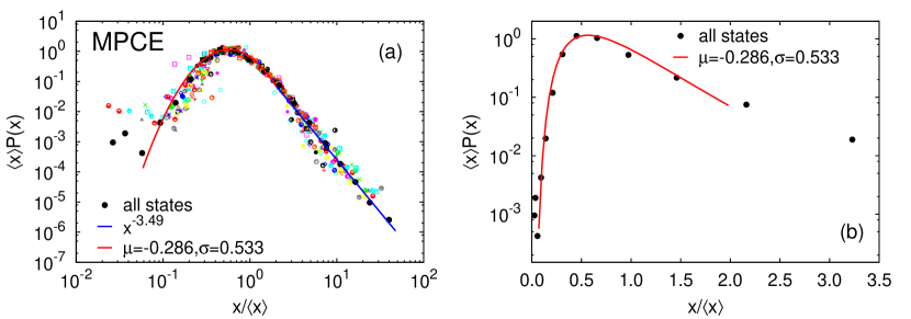
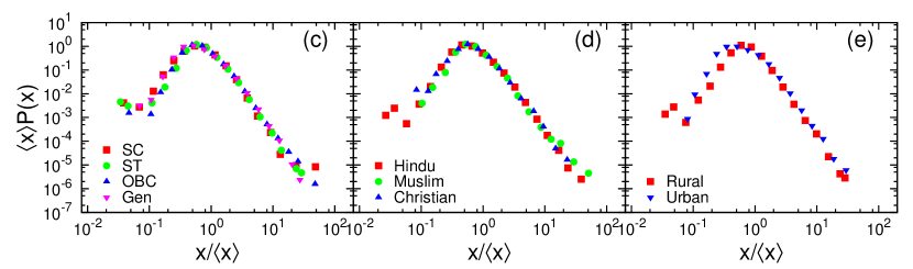
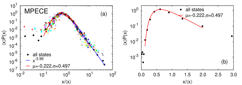
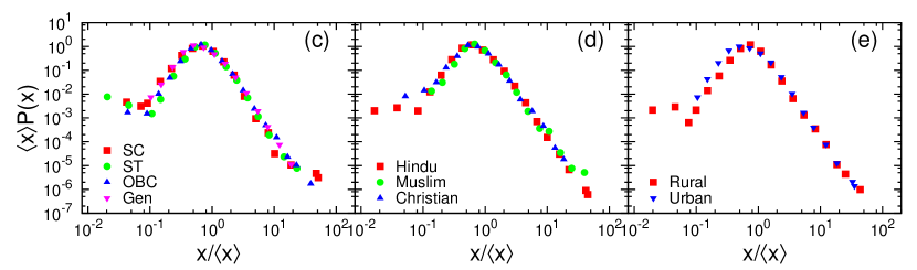
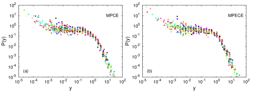
We first compute the probability density (left panels) and then rescale with the mean () for a possible data collapse. In Figs. 1(a) and 2(a), we present the data for all states for MPCE & MPECE respectively. While we acknowledge the fact that the sample size is small for certain states (like Goa, Andaman), we show that the pattern holds true for all states. Also other sociological or geographic factors do not affect it, for which we have significantly large number of data points. We also plotted the full data (black filled circles) and estimated best fits. The bulk of the distribution fits well to a lognormal . For MPCE, the parameters are while for MPECE parameters are . However, for the lowest values, the lognormal fit does not hold. The largest values of consumption expenditure fit well to power law . For MPCE, the decay exponent is and for MPECE, . In Figs. 1(b) and 2(b), we plot the binned full data and the lognormal fit for comparison in log-linear scale. Subsequently, we also show the data filtered according to 3 available parameters: caste (Figs. 1(c) and 2(c)), religion (Figs. 1(d) and 2(d)) and rural-urban divide (Figs. 1(e) and 2(e)). Again the data show excellent scaling collapse, indicating that the basic functional form of the probability distribution is invariant with respect to different states (spatial invariance), caste, religion or rural-urban divide. We also checked that lognormals are the best fits for the rescaled plots (as in panel (b) of Figs. 1 and 2; not shown here).
IV.2 Rescaling the data
In section IV.1, the scaling was done with respect to the average income . Here another type of rescaling is presented. We compute the distribution for the consumption expenditure data normalized with respect to the mean and standard deviation; , where is the sample mean of and is the sample standard deviation. See Figs. 3 for the data collapse in MPCE and MPECE.
IV.3 Inequality along other social dimensions
A basic proposition of this paper is that the distributional features of consumption expenditure are very similar subject to normalization. So far we have considered spatial dimension of consumption inequality. There are interesting features of inequality in terms of other social factors. Labor economists have shown that wage structure varies considerably across spectrum of sex, age and racial backgrounds Hurst;13 . In the present context, a robust feature comes out when we consider similar factors. Surprisingly, inequality in consumption profile across various religious groups and ethnic groups are near identical subject to a scaling factor.
It is important to recognize that income is not the only determinant of well-being even though it has the basic virtue of being easily quantifiable and hence, comparable. The literature has focused on poverty from a multi-dimensional perspective incorporating various other factors Satya;forthcoming . Its theoretical support comes form the capability approach presented by Sen-capability;99 which argues that poverty is manifestation of failure of a person to exercise his/her capabilities to the extent possible. The reasons why such failures exist come in various forms. Religious and ethnic backgrounds constitute two extremely important factors in terms of social and economic barriers. Interestingly we find that the basic statistical features do not change much after normalizing the data. This, in principle, reflects that to understand consumption inequality we need a model that generates dispersion in consumption and consumption profiles need to be multiplicative in nature so that subject to scaling, it generates identical patterns.
Fig. 1(c) shows the normalized probability density functions for data compiled conditional on castes. Next, we study the dispersion in consumption expenditure across religions. Fig. 1(d) clearly shows that the distributional features are very similar across religions. Finally, we have studied dispersion in expenditure across urban versus rural economy. Fig. 1(e) shows that under normalization, similar features prevail. This finding needs some elaboration. As noted above, there is a large literature in labor economics exploring the gap in consumption across various social and ethnic groups and of course, the urban-rural consumption gap has been recognized for long. What these findings suggest is that we do not need different models to explore the dispersion under different conditions. In other words, while it is the case that the economic pie is bigger for some group of people (for example, urban) than their counterpart (say, rural), that indicates absolute inequality. Relative inequalities are of similar nature in both cases. We exploit this property below when we try to come up with a coherent version of the broad picture.
Similar findings persist when we do the same exercise for the MPECE dataset. See Fig. 2.
IV.4 Comparison between the two data sets
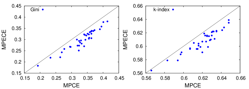
Fig. 4 compares the values of Gini and the -index as computed from the two data sets. Gini index ranges approximately between for MPCE, for MPECE while for k-index, it is for MPCE and for MPECE.
Clearly, MPCE consistently shows more inequality than MPECE in terms of both measures. It is worthwhile to reiterate the definitions here. MPCE is just monthly expenditure on consumption per head of a family. It is calculated as the total consumption expenditure of a household divided by the number of household members. It is important to note that each household member gets equal weight in this formula. On the other hand, MPECE takes into account intra-family heterogeneity. It is monthly per capita equivalent consumption expenditure which is calculated assigning different weights to household members depending on their age. In particular, an adult member gets a higher weight than a child. The main purpose of using equivalence scale is to account for the consumption of goods for common use, like fuel, accommodation etc. Consumption of these goods does to necessarily grow in proportion to household size. Rather, age structure plays crucial role in the consumption.
To see why MPCE is more unequal than MPECE, consider an island with families with size sequence i.e. the -th family has size . To maintain clarity, below the quantities do not carry the island index with the understanding that we are talking only about the -th island. When we make comparisons between islands, we will start indexing the islands by . Let us denote the total expenditure for each family by where the total expenditure is the sum of all individual expenditures on the family members,
| (1) |
Without any loss of generality, let us also assume that the expenditures are ranked so that
| (2) |
By definition, we have the MPCE as of the th family as
| (3) |
where all family members get the same weight and similarly, we can write MPECE as a weighted average of individual expenditures with weights for the -th member,
| (4) | |||||
where in the last line we employed Eq. 3 and the last term combines the dispersion of expenditures from the average. It is noteworthy here that in general,
| (5) |
The reason is that in the definition of MPECE, the adults get a higher weight () and typically the individual expenditure on them would also be high i.e. . Thus there is an upward bias in . This has an immediate corollary which is
| (6) | |||||
which means that for any island the average MPECE would be larger than average MPCE. This can be verified easily from Table 1. Note that Gini coefficient of an island with per capita expenditure profile (where is either MPCE and MPECE) across families can be written as
| (7) | |||||
Now note that, we have (ignoring the index for the island)
| (8) | |||||
Note that by similar logic, we have
| (9) |
In Appendix B we provide a heuristic argument showing that given the ranking of expenditure in Eq. 2, we have
| (10) |
We need two more conditions viz. sufficient dispersion in the expenditure and less dispersion in the terms, both of which should hold in the data. Plugging the above inequality back in the equation for Gini coefficient (Eq. 7), we see that for any island
| (11) |
implying bigger inequality for state-wise comparisons. Since -index is also highly correlated with Gini coefficient, the data shows similar features there as well.
V Dynamical features of inequality
Ref. Kuznets;55 presented a proposition that economies undergoing economic evolution shows an increasing trend in inequality initially before a downward pressure builds on it which brings it down. Such an inverted ‘U’-shaped profile of inequality with respect to average income is known as the Kuznets’ curve. Although the actual time path followed by inequality as a function of per capita income is much more complex than the one originally proposed by Kuznets, it provides a basic intuitive understanding of dynamics of inequality. However, this issue has been controversial as later research suggested that substantial inequality actually affects growth making the causal relationship less robust than it seems. In the same vein, Ref. Deininger;97 shows that by itself economic growth may not directly contribute to the distributional outcomes adversely. Thus from a policy perspective this may not be a major factor. However, one thing that is repeatedly seen is that some inequality seems natural companion of rapid growth. Redistributive policies are also seen to have ambiguous effects on growth. Inequality might grow even at a later stage of development. But evidence has been mixed Atkinson;02 . See also Ref. angle2009kuznets for a theoretical and empirical investigation of this mechanism.
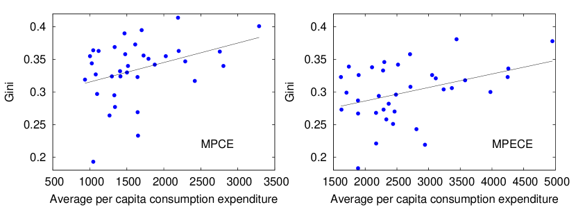
What is of importance to us is the idea that in the initial stages of growth and development, the countries which are on an average more prosperous will be somewhat more unequal than their less prosperous counterparts. Even though it was originally proposed as a time-series idea, we can easily adapt it to a multi-country set-up. One can think of all countries following the same growth path over time (for example, in the spirit of the basic neo-classical growth model, also known as Solow model Acemoglu-growth;09 ). Thus a more prosperous country is nothing but what a poor country will become in future. Here we are making gross simplification in ignoring the roles of institutions Acemoglu-nations-fail;13 . What we gain is a framework to make comparisons between multiple economic entities at the same time. Noting that almost all of the Indian states are substantially large (for example, GDP of Hungary was $137.1 billion in 2014 Worldbank-Hungary;14 and the same for the state Maharashtra is $234.3 billion in the same year Wiki-Maharashtra;14 ; data converted in to dollars based on the current exchange rate), we can do a cross-state comparison. Fig. 5 shows state-wise consumption inequality versus average consumption plot. The regression fit is a liner growth , where is the Gini coefficient and is the average per capita consumption expenditure. For MPCE, and and for MPECE, and .
A very interesting feature of the plot is its apparent adherence to the basic proposition of Kuznets that in the initial growth periods more prosperous states should be more unequal. In case of India, Ref. kanbur2012does presents arguments for and against the finding of such inequality dynamics. Even though cross-sectional estimates refute the claim, time-series estimates show some support to it. In a general context, Ref. chakrabarti2010inequality show how such a feature may arise in a very simple dynamic model depending on relative strength of market correlations to average savings rate. Further study on the evolution of inequality would be able to shade light on how far the data agree with the theory. As has been emphasized by Ref. Atkinson;02 , inequality might increase even in developed economies depending on policies and broadly, institutional factors, it is a non-trivial task to try to predict which path will Indian economy take, both at the aggregate level and at the state level.
VI Interpreting the results
In this section, we present a basic model to understand the empirical findings. The basic point we make here is that consumption profiles across the states can be invariant with respect to average income or other factors. Another important point is that inequality in general increases as average consumption (which is highly correlated with income) increases.
Suppose the economy consists of islands where each island can be identified with a country or in the present context, a state in India. There is a continuum of agents in every island . For simplicity, assume that . Each agent is indexed by . Time is discrete. At every point of time, the agents are endowed with unit labor which are differentiated across workers. They do not value leisure and hence can provide labor inelastically.
There is a continuum of firm in every island which can combine labor to produce output with a standard production function. The aggregate level of production in island is
| (12) |
where is the island-specific state of technology, is the labor endowment of the -th agent in the -th state and is a parameter in the production function. Labor endowment is a constant which is normalized to 1,
| (13) |
We will assume that the technology differs across islands and hence generally, where .
Firms maximize profit,
| (14) | |||||
where is the price of the final good and is the wage rate. In principle, we can normalize the general price level to unity without any loss of generalization. The second equality can be obtained substituting the production function (Eq. 12) in the profit function (Eq. 14) above. By choosing optimal amount of labor, the firms arrive at the following first order condition:
| (15) |
It can be shown that the general price level is nothing but an aggregate function of wage rates,
| (16) |
Given the labor demand equation (Eq. 15), the equilibrium wage rate can be found out by labor market clearing conditions (recall from Eq. 13 that total endowment is 1). Thus in equilibrium, GDP of the -th island is given by
| (17) |
Since the data is on household consumption expenditure, we have to discretize the model. Assume that any generic household is a set of agents )and there are () number of households in each island . We will denote the set of households in each island by as well. For the first household, and for the last household , in each island. To maintain clarity, assume that any agent can belong to only one household. Thus,
| (18) |
where we denote the set of households in a island by .
In island , total production is divided among households to consume. Clearly the contribution () of the th household is
| (19) |
where denotes the distribution of labor endowment on agents. Finally to split the pie i.e. the total production , we assume that the households derive utility from consumption and have a bargaining power proportional to their contribution. This is essentially a Nash bargaining situation. The resultant income distribution would be given by a vector which we denote by .
VI.1 Absolute inequality
Given the income profile which is also the consumption profile as there no savings, we can easily pin down the level of absolute inequality. The easiest way to do it would be to consider the standard deviation,
| (20) |
where denotes expectation operator. Similarly, we could compute the Gini coefficient or the -index. Note that this explains the effects of having better technology on inequality which is explored below. Here, it should be mentioned that the way this model is set up, there is no difference between income and consumption. Thus any income shock will be translated in to an aggregate consumption shock given the perfect sharing mechanism within each family. In reality that is typically not the case Blundell;08 ; Perri;05 . However, we retain this assumption as it makes the model very simple and for present purpose, it suffices to assume no asset market and full within-family insurance.
VI.2 Comparison between state-level inequalities
Consider two islands 1 and 2. Island 1 has a benchmark level of technology, . Island 2 has a better technology, . Then it is easy to show that if all other things remain identical across the islands (productivity distributions, household distributions and production functions), then the income/consumption profile in island 2 is just a blown up version of the same in island 1. It is easy to show that in terms of standard deviation, inequality goes up (see Eq. 20). Thus in terms of variance or standard deviation, the model explains increasing inequality. The basic reason is that these indexes are not scale invariant.
It is also easy to see that upon such normalization, these two consumption profiles coincide. This explains the invariance in consumption distribution upon normalization (Fig. 1). Any measure of relative inequality that is scale invariant i.e. shows zero-degree homogeneity, should be unaffected by such a change. Essentially this refers to the idea that relative inequality across islands should remain unchanged with respect to proportional change in income profile. This potentially presents a problem because in this case the Lorenz curve would not change implying that the Gini coefficient will also not change.
Hence, we introduce one more ingredient. Along with better technology () which increases the size of the pie, let us assume that the households receive stochastic endowments in island where is probability density function with well defined moments. For sake of normalization, let us assume that and . Thus we get two income profiles. For island 1, the profile remains unchanged and .
Let us denote the means of these two series by and . Then the two normalized series and have the same mean but the later is a mean-preserving spread of the former which immediately implies that stochastically dominates in the second order Satya;09 . Therefore, the following inequality holds in terms of the cumulative density functions ,
| (21) |
with strict inequality at some where . This immediately implies that Lorenz dominates (see for example, Ref. Satya;09 ) and hence in terms of Gini coefficient ,
| (22) |
This explains the upward trend of inequality with respect to per capita consumption.
VII Summary and conclusion
In this paper, we have studied spatial invariance of inequality in case of India. We have analyzed data from 35 states and union territories. The data is also available for different castes, religious adherences and urban-rural divide. The main finding of this paper is that under suitable normalization the distributions collapse to a single distribution. This sheds light on the static features of inequality. In particular, it means that state-wise differences in inequality may arise from the differences in average incomes. The spread seems to be fairly constant when that effect is taken away. The lognormal fit of the bulk and power law fit of the tail of the normalized distributions agree with the existing literature.
The generic form of the income distribution is given by a lognormal/gamma bulk and a power law tail. We show here that it is the same for consumption. However, the Pareto exponent is much larger for consumption compared to the income data, reflecting lower consumption inequality than income. By and large, this finding seems to be true in many empirical works. For example, Ref. Perri;05 analyzes cross-sectional income and consumption data for U.S. and shows that income inequality increased substantially during the period 1980-2003 but consumption inequality did increase only by a small amount, reflecting the idea that consumption is less volatile than income at any given point of time. However, it is difficult to pin down an exact relationship between these two measures due to multiple external factors that might affect both consumption and income. A similar argument holds true for wealth as well.
Next we study the growth-inequality nexus and show that usually a higher level of prosperity is associated with a higher level of inequality. Given that India is on the first part of its growth track, this finding is in almost exact agreement with the basic statement of Kuznets’ curve. A brief model is presented to elucidate the idea that a growing pie may due to a better level of technology or riskier projects or more generally, a combination of them. This leads to higher inequality.
This is primarily showing the presence of universality in terms of inequality during the growth process of countries. Further theoretical work would help to explain the causal relationship between growth and rise in inequality, if any. It is also noteworthy that we have considered spatial features only (physical space as in states or in the parameter space of caste, religion or urban-rural divide). The temporal dimension has not been considered which should show both state-wise and aggregate evolution of inequality. However, that lies beyond the scope of the present work.
Appendix A Data Tables
Below we present compiled data on state wise inequality in Table 1. Both the Gini coefficient and the -index have been presented for all states along with average income ().
| Index | State | #Household | MPCE | MPECE | ||||
|---|---|---|---|---|---|---|---|---|
| Gini | Gini | |||||||
| 1 | Jammu & Kashmir | 2726 | 1340.20 | 0.277 | 0.598 | 2332.55 | 0.258 | 0.591 |
| 2 | Himachal Pradesh | 2043 | 1726.27 | 0.356 | 0.628 | 2713.30 | 0.308 | 0.609 |
| 3 | Punjab | 3117 | 1877.41 | 0.342 | 0.623 | 3113.03 | 0.321 | 0.616 |
| 4 | Chandigar | 305 | 3288.60 | 0.401 | 0.648 | 4952.62 | 0.378 | 0.639 |
| 5 | Uttaranchal | 1780 | 1413.57 | 0.324 | 0.615 | 2289.23 | 0.273 | 0.596 |
| 6 | Haryana | 2620 | 1792.95 | 0.351 | 0.625 | 3054.84 | 0.326 | 0.616 |
| 7 | Delhi | 957 | 2805.90 | 0.340 | 0.622 | 4246.83 | 0.323 | 0.619 |
| 8 | Rajasthan | 4138 | 1408.53 | 0.332 | 0.618 | 2370.31 | 0.282 | 0.599 |
| 9 | Uttar Pradesh | 8993 | 1080.05 | 0.327 | 0.616 | 1885.53 | 0.287 | 0.601 |
| 10 | Bihar | 4568 | 934.70 | 0.319 | 0.614 | 1624.77 | 0.273 | 0.596 |
| 11 | Sikkim | 768 | 1644.50 | 0.323 | 0.620 | 2438.57 | 0.251 | 0.591 |
| 12 | Arunachal Pradesh | 1642 | 1297.71 | 0.324 | 0.616 | 2213.81 | 0.294 | 0.604 |
| 13 | Nagaland | 1024 | 1651.50 | 0.233 | 0.583 | 2942.54 | 0.219 | 0.579 |
| 14 | Manipur | 2558 | 1046.59 | 0.193 | 0.566 | 1886.58 | 0.183 | 0.564 |
| 15 | Mizoram | 1528 | 1646.45 | 0.269 | 0.597 | 2808.10 | 0.243 | 0.588 |
| 16 | Tripura | 1856 | 1331.25 | 0.295 | 0.607 | 2170.16 | 0.268 | 0.596 |
| 17 | Meghalaya | 1272 | 1266.10 | 0.264 | 0.594 | 2171.71 | 0.221 | 0.579 |
| 18 | Assam | 3448 | 1098.20 | 0.297 | 0.607 | 1887.38 | 0.267 | 0.597 |
| 19 | West Bengal | 6324 | 1335.42 | 0.369 | 0.635 | 2107.57 | 0.338 | 0.622 |
| 20 | Jharkhand | 2751 | 1026.32 | 0.344 | 0.624 | 1704.10 | 0.299 | 0.607 |
| 21 | Orissa | 4031 | 1001.90 | 0.355 | 0.627 | 1616.64 | 0.323 | 0.615 |
| 22 | Chattisgarh | 2230 | 1045.88 | 0.364 | 0.631 | 1741.39 | 0.339 | 0.622 |
| 23 | Madhya Pradesh | 4705 | 1118.79 | 0.363 | 0.630 | 1896.47 | 0.326 | 0.616 |
| 24 | Gujarat | 3425 | 1501.83 | 0.330 | 0.620 | 2484.72 | 0.296 | 0.607 |
| 25 | Daman & Diu | 128 | 2026.93 | 0.355 | 0.629 | 3236.79 | 0.304 | 0.610 |
| 26 | D & N Haveli | 192 | 1515.47 | 0.340 | 0.626 | 2462.95 | 0.270 | 0.599 |
| 27 | Maharashtra | 8005 | 1700.64 | 0.395 | 0.643 | 2706.95 | 0.358 | 0.628 |
| 28 | Andhra Pradesh | 6889 | 1613.82 | 0.373 | 0.635 | 2517.41 | 0.342 | 0.623 |
| 29 | Karnataka | 4074 | 1468.72 | 0.390 | 0.641 | 2300.90 | 0.346 | 0.624 |
| 30 | Goa | 447 | 2419.38 | 0.317 | 0.611 | 3975.30 | 0.300 | 0.605 |
| 31 | Lakshadweep | 184 | 2201.62 | 0.363 | 0.633 | 3366.33 | 0.306 | 0.611 |
| 32 | Kerala | 4455 | 2192.06 | 0.414 | 0.648 | 3440.41 | 0.381 | 0.635 |
| 33 | Tamil Nadu | 6639 | 1478.30 | 0.358 | 0.630 | 2281.49 | 0.333 | 0.621 |
| 34 | Pondicherry | 576 | 2289.77 | 0.347 | 0.625 | 3575.46 | 0.318 | 0.615 |
| 35 | A & N Island | 559 | 2757.06 | 0.362 | 0.632 | 4257.64 | 0.336 | 0.622 |
In the following we also present, caste, religion and location-based inequality measures along with their average prosperity.
| Index | Caste | #Household | MPCE | MPECE | ||||
|---|---|---|---|---|---|---|---|---|
| Gini | Gini | |||||||
| 1 | ST | 12928 | 1199.02 | 0.339 | 0.621 | 2031.68 | 0.313 | 0.611 |
| 2 | SC | 16181 | 1114.59 | 0.329 | 0.617 | 1853.54 | 0.294 | 0.603 |
| 3 | OBC | 37872 | 1316.96 | 0.352 | 0.626 | 2164.61 | 0.315 | 0.612 |
| 9 | General | 33912 | 1817.78 | 0.383 | 0.639 | 2902.85 | 0.346 | 0.625 |
| Index | Religion | #Household | MPCE | MPECE | ||||
|---|---|---|---|---|---|---|---|---|
| Gini | Gini | |||||||
| 1 | Hindu | 76949 | 1429.07 | 0.376 | 0.636 | 2311.01 | 0.339 | 0.621 |
| 2 | Muslim | 12439 | 1245.50 | 0.350 | 0.624 | 2117.70 | 0.310 | 0.610 |
| 3 | Christian | 6948 | 1688.70 | 0.355 | 0.628 | 2799.80 | 0.320 | 0.614 |
| 4 | Other religion | 4598 | 1718.93 | 0.366 | 0.632 | 2857.81 | 0.337 | 0.621 |
| Index | #Household | MPCE | MPECE | |||||
|---|---|---|---|---|---|---|---|---|
| Gini | Gini | |||||||
| 0 | Rural | 41828 | 1865.76 | 0.384 | 0.638 | 2942.37 | 0.347 | 0.625 |
| 1 | Urban | 59129 | 1134.62 | 0.313 | 0.610 | 1923.88 | 0.286 | 0.600 |
Appendix B Relative inequality
Recall that (Eq. 8 and 9) we have
| (23) |
and
| (24) |
For simplicity, let us assume that . Then
| (25) |
Let us denote the relationship between and by . We want to check if is or . We can write,
| (26) |
which can be simplified to
| (27) |
or
| (28) |
The above expression can be rewritten as
| (29) |
From Eq. 2 (without loss of generalization, assuming that the family sizes are identical), the above relationship clearly shows that is i.e.
| (30) |
This implies,
| (31) |
References
- [1] K. J. Arrow, S. Bowles, and S. N. Durlauf. Meritocracy and economic inequality. Princeton Univ. Press, 2000.
- [2] J. E. Stiglitz. The price of inequality: How today’s divided society endangers our future. WW Norton & Company, 2012.
- [3] A. Chatterjee. Socio-economic inequalities: a statistical physics perspective. In F. Abergel, H. Aoyama, B. K. Chakrabarti, A. Chakraborti, and A. Ghosh, editors, Econophysics and Data Driven Modelling of Market Dynamics, pages 287–324. New Economic Windows, Springer, Milan, 2015.
- [4] A. Chatterjee, A. Ghosh, J. I. Inoue, and B. K. Chakrabarti. Social inequality: from data to statistical physics modeling. arXiv:1507.02445, 2015.
- [5] T. Piketty. Capital in the Twenty-first Century. Harvard Univ. Press, 2014.
- [6] B. K. Chakrabarti, A. Chakraborti, S. R. Chakravarty, and A. Chatterjee. Econophysics of income and wealth distributions. Cambridge Univ. Press, Cambridge, 2013.
- [7] I. I. Eliazar and M. H. Cohen. On social inequality: Analyzing the rich-poor disparity. Physica A, 410:148–158, 2014.
- [8] R. Blundell, L. Pistaferri, and I. Preston. Consumption inequality and partial insurance. Am. Econ. Review, 98-5:1887–1921, 2008.
- [9] V. Pareto. Cours d’economie politique. Rouge, Lausanne, 1897.
- [10] E. W. Montroll and M. F. Shlesinger. On 1/f noise and other distributions with long tails. Proc. Natl. Acad. Sci., 79:3380–3383, 1982.
- [11] C. Gini. Measurement of inequality of incomes. Econ. J., 31(121):124–126, 1921.
- [12] R.V. Hogg, J.W. Mckean, and A.T. Craig. Introduction to mathematical statistics. Pearson Education, Delhi, 2007.
- [13] A. A. Drăgulescu and V. M. Yakovenko. Exponential and power-law probability distributions of wealth and income in the united kingdom and the united states. Physica A, 299(1):213–221, 2001.
- [14] A. Chatterjee, S. Yarlagadda, and B. K. Chakrabarti, editors. Econophysics of Wealth Distributions. New Economic Windows Series, Springer-Verlag, Milan, 2005.
- [15] A. Chatterjee and B. K. Chakrabarti. Kinetic exchange models for income and wealth distributions. Eur. Phys. J. B, 60:135–149, 2007.
- [16] A. Banerjee and V.M. Yakovenko. Universal patterns of inequality. New J. Phys., 12:075032, 2010.
- [17] V.M. Yakovenko and J. Barkley Rosser Jr. Statistical mechanics of money, wealth and income. Rev. Mod. Phys., 81:1703–1725, 2009.
- [18] P. Richmond, S. Hutzler, R. Coelho, and P. Repetowicz. A review of empirical studies and models of income distributions in society. In B. K. Chakrabarti, A. Chakraborti, and A. Chatterjee, editors, Econophysics and Sociophysics: Trends and Perspectives, pages 131–159. Wiley-VCH, Weinheim, 2007.
- [19] S. Sinha. Evidence for power-law tail of the wealth distribution in india. Physica A, 359:555–562, 2006.
- [20] A. Jayadev. A power law tail in india’s wealth distribution: Evidence from survey data. Physica A, 387(1):270–276, 2008.
- [21] S. Lawrence, Q. Liu, and V. M. Yakovenko. Global inequality in energy consumption from 1980 to 2010. Entropy, 15(12):5565–5579, 2013.
- [22] T. Mizuno, M. Toriyama, T. Terano, and M. Takayasu. Pareto law of the expenditure of a person in convenience stores. Physica A, 387(15):3931–3935, 2008.
- [23] E. Battistin, R. Blundell, and A. Lewbel. Why is consumption more log normal than income? gibrat’s law revisited. J. Polit. Econ., 117(6):1140–1154, 2009.
- [24] G. Fagiolo, L. Alessi, M. Barigozzi, and M. Capasso. On the distributional properties of household consumption expenditures: the case of italy. Empirical Econ., 38(3):717–741, 2010.
- [25] A. Ghosh, K. Gangopadhyay, and B. Basu. Consumer expenditure distribution in india, 1983–2007: Evidence of a long pareto tail. Physica A, 390(1):83–97, 2011.
- [26] S. Fortunato and C. Castellano. Scaling and universality in proportional elections. Phys. Rev. Lett., 99(13):138701, 2007.
- [27] A. Chatterjee, M. Mitrović, and S. Fortunato. Universality in voting behavior: an empirical analysis. Sci. Rep., 3:1049, 2013.
- [28] H. D. Rozenfeld, D. Rybski, J. S. Andrade, M. Batty, H. E. Stanley, and H. A. Makse. Laws of population growth. Proc. Natl. Acad. Sci., 105(48):18702–18707, 2008.
- [29] M. H. R. Stanley, L. A. N. Amaral, S. V. Buldyrev, S. Havlin, H. Leschhorn, P. Maass, M. A. Salinger, and H. E. Stanley. Scaling behaviour in the growth of companies. Nature, 379(6568):804–806, 1996.
- [30] A. M. Petersen, J. Tenenbaum, S. Havlin, and H. E. Stanley. Statistical laws governing fluctuations in word use from word birth to word death. Sci. Rep., 2:313, 2012.
- [31] C. Castellano, S. Fortunato, and V. Loreto. Statistical physics of social dynamics. Rev. Mod. Phys., 81:591–646, 2009.
- [32] P. Sen and B. K. Chakrabarti. Sociophysics: An Introduction. Oxford Univ. Press, Oxford, 2014.
- [33] Household Consumer Expenditure 66th Round from the National Sample Survey Office (NSSO), 2009-2010. http://mail.mospi.gov.in/index.php/catalog/CEXP.
- [34] A. J. M. Hagenaars, K. De Vos, and M. A. Zaidi. Poverty statistics in the late 1980s: Research based on micro-data. Office for Official Publications of the European Communities, 1996.
- [35] S. R. Chakravarty. Inequality, Polarization and Poverty: Advances in Distributional Analysis. Springer, New York, 2009.
- [36] A. Ghosh, N. Chattopadhyay, and B. K. Chakrabarti. Inequality in societies, academic institutions and science journals: Gini and k-indices. Physica A, 410:30–34, 2014.
- [37] J-I. Inoue, A. Ghosh, A. Chatterjee, and B. K. Chakrabarti. Measuring social inequality with quantitative methodology: analytical estimates and empirical data analysis by gini and indices. Physica A, 429:184–204, 2015.
- [38] G. Datt and M. M. Ravallion. Why have some indian states done better than others at reducing rural poverty? Economica, 65(1):17–38, 1992.
- [39] P. Mishra and A. Parikh. Household consumer expenditure inequalities in india: a decomposition analysis. Rev. Income Wealth, 410:225–236, 1992.
- [40] C. T. Hsieh, E. Hurst, C. I. Jones, and P. J. Klenow. The Allocation of Talent and U.S. Economic Growth. working paper.
- [41] S. R. Chakravarty and N. Chattopadhyay. Multidimensional poverty and material deprivation: A theoretical analysis. In C. D’Ambrosio, editor, Handbook of Research on Economic and Social Well-Being. Edward Elgar Publishing: Northampton, MA, 2015.
- [42] A. Sen. Development as Freedom. Knopf, New York, 1999.
- [43] S. Kuznetz. Economic growth and income inequality. Am. Econ. Review, 45:1–28, 1955.
- [44] K. Deininger and L. Squire. Economic growth and income inequality: reexamining the links. Finance and development, March, 2007.
- [45] T. Atkinson. Is rising income inequality inevitable? a critique of the ‘transatlantic consensus’. In P. Townsend and D. Gordon, editors, World Poverty. U. Chicago Press, 2002.
- [46] J. Angle, F. Nielsen, and E. Scalas. The kuznets curve and the inequality process. In B. Basu, B. K. Chakrabarti, S. R. Chakravarty, and K. Gangopadhyay, editors, Econophysics and economics of games, social choices and quantitative techniques, pages 125–138. Springer, Milan, 2009.
- [47] D. Acemoglu. Introduction to Modern Economic Growth. Princeton University Press, New York, 2009.
- [48] D. Acemoglu and J. Robinson. Why Nations Fail: The Origins of Power, Prosperity and Poverty. Corwn Business, 2013.
- [49] Hungary, Data, The World Bank. http://data.worldbank.org/country/hungary.
- [50] Wikipedia – List of Indian states by GDP. https://en.wikipedia.org/wiki/List-of-Indian-states-by-GDP.
- [51] R. Kanbur. Does kuznets still matter? Policy-Making for Indian Planning: Essays on Contemporary Issues in Honor of Montek S. Ahluwalia, 1(1):5–128, 2012.
- [52] A. S. Chakrabarti and B. K. Chakrabarti. Inequality reversal: Effects of the savings propensity and correlated returns. Physica A, 389(17):3572–3579, 2010.
- [53] D. Krueger and F. Perri. Does income inequality lead to consumption inequality? evidence and theory. Rev. Econ. Studies, 73(1):163–193, 2006.