Disentangling multipole contributions to collective excitations in fullerenes

Abstract

Angular resolved electron energy-loss spectroscopy (EELS) gives access to the momentum and the energy dispersion of electronic excitations and allows to explore the transition from individual to collective excitations. Dimensionality and geometry play thereby a key role. As a prototypical example we analyze theoretically the case of Buckminster fullerene C₆₀ using ab initio calculations based on the time-dependent density-functional theory. Utilizing the non-negative matrix factorization method, multipole contributions to various collective modes are isolated, imaged in real space, and their energy and momentum dependencies are traced. A possible experiment is suggested to access the multipolar excitations selectively via EELS with electron vortex (twisted) beams. Furthermore, we construct an accurate analytical model for the response function. Both the model and the ab initio cross sections are in excellent agreement with recent experimental data.

Plasmonics, a highly active field at the intersection of nanophotonics, material science and nanophysics Schuller et al. (2010), has a long history dating back to the original work of Gustav Mie on light scattering from spherical colloid particles Mie (1908); Halas et al. (2011). For extended systems the plasmon response occurs at a frequency set by the carrier density while in a finite system topology and finite-size quantum effects play a key role. E.g., for a nano-shell Liz-Marzan (2006); Jain and El-Sayed (2007); Prodan et al. (2003) in addition to the volume mode, two coupled ultraviolet surface plasmons arise having significant contributions from higher multipoles, as demonstrated below. Such excitations can be accessed by optical means as well as by electron energy-loss spectroscopy (EELS) Egerton (2009); García de Abajo (2010). Particle-hole ($p\mathchar 45\relax h$) excitations and collective modes may “live” in overlapping momentum-energy domains and couple in a size-dependent way that cannot be understood classically Yannouleas and Broglia (1992); Alasia et al. (1994); Moskalenko et al. (2012). Giant plasmon resonances were measured in buckminster fullerene C₆₀ Sohmen et al. (1992); Burose et al. (1993); Bolognesi et al. (2012); Hertel et al. (1992); Scully et al. (2005); Reinköster et al. (2004) and explained, e.g., by assuming C₆₀ to have a constant density of electrons confined to a shell with inner ($R_{1}$) and outer ($R_{2}$) radii (the spherical shell model) Östling et al. (1996); Vasvári (1996); Verkhovtsev et al. (2012a). Refinements in terms of a semi-classical approximation (SCA) incorporate the quantum-mechanical density extending out of the shell $R_{1}<r<R_{2}$ (so-called spill-out density Esteban et al. (2012)). Time-dependent density functional theory (TDDFT) Prodan and Nordlander (2003); Marques and Gross (2004); Esteban et al. (2012) was also employed in a number of calculations Bauernschmitt et al. (1998); Madjet et al. (2008); Maurat et al. (2009), however, most of them use the jellium model, i.e., the ionic structure is smeared out to a uniform positive background.
We present here, to our knowledge, the first atomistic full-fledge TDDFT calculations for EELS from C₆₀ at finite momentum transfer. We demonstrate the necessity of the full ab-initio approach by unraveling the nature of the various contributing plasmonic modes and their multipolar character. This is achieved by analyzing and categorizing the ab initio results by means of the non-negative matrix factorization method Lee and Seung (1999). The results are in line with recent experimental findings Verkhovtsev et al. (2012b). The analysis also allows for constructing an accurate analytical model response function.

In first Born approximation for the triply-differential cross section (TDCS) for detecting an electron with momentum $\mathbf{p}_{f}$, i.e., measuring its solid scattering angle $\mathrm{d}\Omega$ and energy $\epsilon_{\mathbf{p}_{f}}$ is

$$\frac{\mathrm{d}^{3}\sigma}{\mathrm{d}\omega\mathrm{d}\Omega}=\frac{4\gamma^{2}}{q^{4}}\frac{p_{f}}{p_{i}}S(\mathbf{q},\omega)\ .$$ (1)

Here, $\mathbf{p}_{i}$ is the incidence momentum corresponding to an energy $\epsilon_{\mathbf{p}_{i}}$, $\gamma$ is the Lorenz factor, $\mathbf{q}=\mathbf{p}_{f}-\mathbf{p}_{i}$ is the momentum transfer, and $\omega=\epsilon_{\mathbf{p}_{f}}-\epsilon_{\mathbf{p}_{i}}$ (atomic units are used throughout). $S(\mathbf{q},\omega)$ is the dynamical structure factor akin solely to the target Giuliani and Vignale (2005).

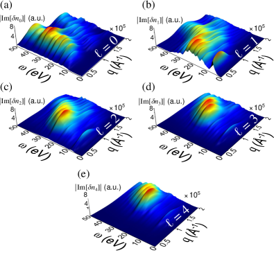
Figure 1: (Color online) The $\ell$-resolved constituents of the dynamical structure factor of C₆₀, $|\mathrm{Im}[\delta n_{\ell}(q,\omega)]|$ for (a) $\ell=0$, (b) $\ell=1$, (c) $\ell=2$, (d) $\ell=3$, and (e) $\ell=4$. The C₆₀ molecule was treated in standard truncated icosahedric geometry with bond lengths $r_{\mathrm{C-C}}=1.445$ Å and $r_{\mathrm{C=C}}=1.390$ Å.

The fluctuation-dissipation Giuliani and Vignale (2005) theorem links $S(\mathbf{q},\omega)$ with the non-local, retarded density-density linear response function $\chi^{\mathrm{R}}(\mathbf{r},\mathbf{r}^{\prime};t-t^{\prime})$ Onida et al. (2002); Giuliani and Vignale (2005); Marques et al. (2012) via $S(\mathbf{q},\omega)=-(1/\pi)\mathrm{Im}[\chi^{\mathrm{R}}(\mathbf{q},-\mathbf{q};\omega)]$. On the other hand, $\chi^{\mathrm{R}}(\mathbf{r},\mathbf{r}^{\prime};t-t^{\prime})$ describes the change in the system density $\delta n(\mathbf{r},t)$ upon a small perturbing potential $\delta\varphi(\mathbf{r},t)$, i.e.

$$\delta n(\mathbf{r},t)=-\int^{\infty}_{-\infty}\!\mathrm{d}t^{\prime}\!\int\!\mathrm{d}\mathbf{r}^{\prime}\,\chi^{\mathrm{R}}(\mathbf{r},\mathbf{r}^{\prime};t-t^{\prime})\delta\varphi(\mathbf{r}^{\prime},t^{\prime})\ .$$ (2)

The response function is determined by evaluating the density variation with tunable perturbations, as accomplished via TDDFT which delivers $\delta n(\mathbf{r},t)$ upon solving the time-dependent Kohn-Sham (KS) equations Note (1).

Along this line, we utilized the Octopus package Marques et al. (2003); Andrade et al. (2012), and propagated the KS equations. Kohn-Sham states are represented on a uniform real space grid Andrade et al. (2015) (0.2 Å grid spacing) confined to a sphere with 10 Å radius. For the ground state we checked the performance of different typical functionals and found that the local-density approximation (LDA) improved by self-interaction correction (SIC) yields fairly good results. The HOMO (-9.2 eV) is located slightly too low with respect to the experimental value (-7.6 eV) Hertel et al. (1992). The band width (which is typically underestimated in DFT) within the LDA+SIC scheme is the largest for the tested functionals Note (2). LDA-type Troullier-Martins pseudopotentials are used to incorporate the influence of the two core electrons per C atom, such that only the 240 valence electrons accounted for. Gaussian smearing has been employed to deal with the degeneracy of the HOMO. In gas-phase the molecules are randomly oriented. Hence, we have to evaluate the spherically averaged structure factor $S(q,\omega)$. Technically, this can be accomplished by choosing the perturbation $\delta\varphi(\mathbf{r},t)=I_{0}\delta(t)j_{\ell}(qr)Y^{*}_{\ell m}(\Omega_{\mathbf{r}})$ Sakko et al. (2010) where $j_{\ell}$ is the spherical Bessel function and $Y_{\ell m}$ is the spherical harmonic. The perturbation strength lies with $I_{0}=0.01$ a.u. well within the regime of linear response. The perturbed states are then propagated by the AETRS propagator Castro et al. (2004) up to $T=20~{}\hbar$/eV with a time step of $\Delta t=2\times 10^{-3}\hbar$/eV, covering the range from $0.31$ eV to $3142$ eV in frequency space. The large simulation box ensured the adequate representation of excited states. A mask was multiplied to the Kohn-Sham states at each time step in order smoothly absorb contributions above the ionization threshold. From the density variation $\delta n(\mathbf{r},t)=n(\mathbf{r},t)-n(\mathbf{r},t=0)$, $\delta n_{\ell m}(q,t)=\int\mathrm{d}\mathbf{r}\,\delta n(\mathbf{r},t)j_{\ell}(qr)Y_{\ell m}(\Omega_{\mathbf{r}})$ is then computed in each time step and Fourier transformed to $\delta n_{\ell m}(q,\omega)$ allowing to determine $S(q,\omega)$ as

$$S(q,\omega)=-\frac{4}{I_{0}}\sum^{\ell_{\mathrm{max}}}_{\ell=0}\sum^{\ell}_{m=-\ell}\mathrm{Im}\left[\delta n_{\ell m}(q,\omega)\right]\ .$$ (3)

The $m$-dependence is subsidiary. To a good approximation henceforth $m=0$ (cf. Eq. (3)). It is sufficient to consider $|\mathrm{Im}[\delta n_{\ell}(q,\omega)]|\equiv-\mathrm{Im}[\delta n_{\ell,m=0}(q,\omega)]$ which stands for the $\ell$-resolved dynamical structure factor depicted in Fig. 1. For $q\rightarrow 0$ (in the optical limit) the dipolar term is clearly dominant over higher multipoles.
According to the shell model Verkhovtsev et al. (2012a) the C₆₀ molecule possesses a volume plasmon mode ($\ell=0$ and radial density oscillation with one node), a symmetric surface mode ($\ell\geq 1$ and no radial oscillation), and an anti-symmetric surface mode ($\ell\geq 1$ and one radial node). We denote these modes by V, S1 and S2, respectively. The plasmon energies are derived as $\omega_{\mathrm{V}}=\sqrt{3/r^{3}_{s}}$, $\omega^{2}_{\mathrm{S(1,2)},\ell}=\frac{\omega^{2}_{\mathrm{V}}}{2}\big{[}1\mp\frac{1}{2\ell+1}\sqrt{1+4\ell(\ell+1)(R_{1}/R_{2})^{(2\ell+1)}}\big{]}$. Inspecting the $\ell=1$ panel the two surface modes may be identified around $q\sim 0.3$ Å^-1, $\omega\sim 20$ eV and $q\sim 1$ Å^-1, $\omega\sim 40$ eV.
As evident from Fig. 1, for higher $q$ plasmonic modes ($\mathrm{S1,S2,V}$) seem to merge and attain various multipoles contributions. This is a manifestation of electronic transitions between the single-particle states with different angular momentum Feng et al. (2008); Pavlyukh and Berakdar (2009, 2011). Thus, the question arises of how to disentangle these modes and to unravel their multipolar nature.

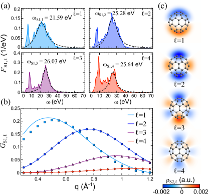
Figure 2: (Color online) (a) Frequency-dependent part of the S1 modes obtained from the NMF (shaded curves) with fits (dashed lines). For plasmon features we concentrate on the region $\omega>18$ eV. (b) $q$-dependent part of the S1 modes from the NMF (solid lines) along with fits using the model fluctuation density (symbols). (c) Model fluctuation density $\rho_{\mathrm{S1,\ell}}$ in a plane cut through the center of the molecule for $\ell$ ranging from 1 (top) to 4 (bottom).

A suitable mathematical tool to tackle this task is the non-negative matrix factorization (NMF), which is extensively used, e. g., for face recognition algorithms Lee and Seung (1999). Applied to our problem, the NMF delivers two functions $F_{i}(\omega)\geq 0$ and $G_{i}(q)\geq 0$ that enter the density response as $|\delta n_{\ell}(q,\omega)|=\sum_{i}F_{i}(\omega)G_{i}(q)$ (see appendix A). This structure follows namely from the Lehmann representation of $\chi^{\mathrm{R}}(\mathbf{r},\mathbf{r}^{\prime};\omega)$ as

$$\chi^{\mathrm{R}}(\mathbf{r},\mathbf{r}^{\prime};\omega)=\sum_{\alpha}\xi_{\alpha}(\omega)\rho_{\alpha}(\mathbf{r})\rho_{\alpha}(\mathbf{r}^{\prime}),\quad\xi_{\alpha}(\omega)=\frac{2E_{\alpha}}{(\omega+\mathrm{i}\Gamma_{\alpha})^{2}-E^{2}_{\alpha}}\$$ (4)

where $\rho_{\alpha}$ is the real fluctuation density corresponding to a transition from the ground to an excited many-body state labelled by $\alpha$ (with excitation energy $E_{\alpha}$), and $\Gamma_{\alpha}$ is the line width. Assuming spherical symmetry, excitations have angular ($\ell$) and radial ($\nu$) components. Expanding $\rho_{\alpha}(\mathbf{r})\rho_{\alpha}(\mathbf{r}^{\prime})=\sum_{\ell m}R_{\nu,\ell}(r)R_{\nu,\ell}(r^{\prime})Y_{\ell m}(\Omega_{\mathbf{r}})Y^{*}_{\ell m}(\Omega_{\mathbf{r}^{\prime}})$ Eq. (4) implies for the structure factor

$$S(q,\omega)=\sum_{\nu\ell}(2\ell+1)F_{\nu,\ell}(\omega)G_{\nu,\ell}(q),$$

$$F_{\nu,\ell}(\omega)=\mathrm{Im}[\xi_{\nu,\ell}(\omega)],\quad G_{\nu,\ell}(q)=\left(\int^{\infty}_{0}\!\mathrm{d}r\,r^{2}R_{\nu,\ell}(r)j_{\ell}(qr)\right)^{2}.$$

In full generality the sum (4) contains infinite number of terms corresponding to the infinite number of excited states. For homogeneous electron gas plasmons are strongly damped when their momentum enters the $p\mathchar 45\relax h$ continuum, where the non-interacting structure factor $S^{(0)}(q,\omega)>0$. For electrons confined to a spherical shell the momentum can be represented by a magnitude $q$ and an angular momentum $\ell$. To mark the effective region $q_{\mathrm{max}}$ and $\ell_{\mathrm{max}}$ in which plasmon modes exist, we estimate the transverse momentum as $2\ell\pi/R$ (with radius $R$) and compare it to the critical momentum $q_{\mathrm{crit}}=0.559k_{\mathrm{F}}$ Stefanucci and Leeuwen (2013) (the Fermi momentum is $k_{\mathrm{F}}=(9\pi/4)^{1/4}r^{-1}_{s}$). We find so a critical $\ell\sim 3$. Thus, any collective excitation beyond $\ell_{\mathrm{max}}=4$ will be suppressed. For a complementary picture, we analyzed $S^{(0)}(q,\omega)$ in SCA Pavlyukh et al. (2012), for which the electron density enters as a central ingredient (we take the spherically-averaged DFT density $n_{0}(r)$) Note (3). This allows to estimate for which $q$ the $p\mathchar 45\relax h$ pairs dominate the spectrum for each $\ell$ separately. For $\ell_{\mathrm{max}}=4$ we find the $p\mathchar 45\relax h$ domain at $q\gtrsim 1.2$ Å^-1. Note that due to geometrical confinement plasmons and $p\mathchar 45\relax h$ excitations intersect each other and couple so significantly.
Now we separate the response into $\nu=\text{S1}$ (Fig. 2) and $\nu=\text{S2}$ (Fig. 3) for $\ell\geq 1$, while the mode $\nu=\text{V}$ can be found from $\ell=0$ density component (Fig. 4). The onset of $p\mathchar 45\relax h$ excitations is also present in the spectra.

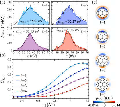
Figure 3: (Color online) (a) Frequency-dependent part of the S2 modes from the NMF (shaded curves) and corresponding fits (dashed lines). For the latter, no constraint has been imposed on the frequency range. (b) $q$-dependent part of the S2 modes from the NMF (solid lines) and fits (symbols). (c) Model fluctuation density $\rho_{\mathrm{S2,\ell}}$ as in Fig. 2.

The plasmon frequencies $\omega_{\nu,\ell}$ are identified from the maximum of the $\omega$-dependence spectra as obtained by the NMF in the form $F^{\mathrm{fit}}_{\nu,\ell}(\omega)=\mathrm{Im}[2\omega_{\nu,\ell}/((\omega+\mathrm{i}\Gamma_{\nu,\ell})^{2}-\omega^{2}_{\nu,\ell})]$. Inspecting Fig. 2(a), we find the dipole plasmon at $\omega_{\mathrm{S1},1}\simeq 21.59$ eV, this is a well established value. Increasing $\ell$ shifts the peak to larger energies (in line with the shell model); the sharp peak around 7.5 eV, which is known to consist of a series of $p\mathchar 45\relax h$ excitations Moskalenko et al. (2012), gains spectral weight until it dominates for $\ell=4$. Abundance of large angular momentum states around HOMO-LUMO gap Pavlyukh and Berakdar (2011) increases the number of channels for high-multipole electronic transitions and is responsible for the peak’s enhancement. The plasmon frequency $\omega_{\mathrm{S1},4}=25.64$ eV on the other hand is smaller than $\omega_{\mathrm{S1},3}=26.03$ eV. This demonstrates the limitations of the SCA.

The radial profile of the density oscillations $R_{\nu,\ell}(r)$ can be inferred from $G_{\nu,\ell}(q)$ in that we assume $R^{\mathrm{fit}}_{\mathrm{S1},\ell}(r)=A_{\ell}r\exp[-(r-r_{\ell})^{2}/2\sigma^{2}_{\ell}]$ and extract the parameters $(A_{\ell},r_{\ell},\sigma_{\ell})$ for which $\big{\|}G^{\mathrm{}}_{\mathrm{S1},\ell}(q)-\left(\int^{\infty}_{0}\!\mathrm{d}r\,r^{2}R^{\mathrm{fit}}_{\mathrm{S1},\ell}(r)j_{\ell}(qr)\right)^{2}\big{\|}$ is minimized. The effective fluctuation densities are then given by $\rho_{\mathrm{S1},\ell}(\mathbf{r})=R_{\mathrm{S1},\ell}(r)Y_{\ell 0}(\Omega_{\mathbf{r}})$, cf. figure 2(c).

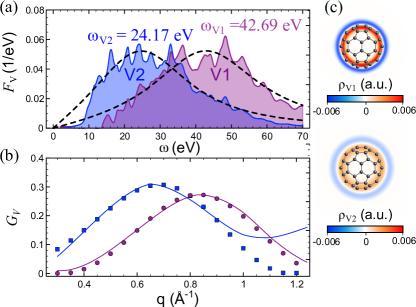
Figure 4: (Color online) (a) Frequency-dependent part of the V1 (blue shaded curve) and V2 (purple shaded curve) mode from the NMF along with corresponding fits (dashed lines). Fitting has been carried out in the complete frequency range. (b) $q$-dependent part of the V1 and V2 modes from the NMF (solid lines) and fits (symbols). (c) Model fluctuation densities in the same plane as in Fig. 2.

Analogous procedure for S2 modes (Fig. 3) reveals a decrease of the plasmon energies in qualitative agreement with Ref. Bolognesi et al. (2012). However, the dispersion is less pronounced than in the shell model. To characterize the fluctuation densities, we use an Ansatz containing a node $R^{\mathrm{fit}}_{\mathrm{S2},\ell}(r)=A_{\ell}r(1-r/r^{(0)}_{\ell})\exp[-(r-r_{\ell})^{2}/2\sigma^{2}_{\ell}]$ and determine the parameters as to match $G_{\mathrm{S2},\ell}(q)$ (Fig. 3(b)). The spatial structure of the plasmon oscillation is shown in Fig. 3(c).

A common and physically intuitive feature of the S1 and S2 modes is that the spatial extend of the fluctuation density is growing with $\ell$. This is a consequence of the increasing centrifugal force, ”pushing” the oscillation away from the center.

Applying the NMF with two components to $|\mathrm{Im}[\delta n_{0}(q,\omega)]|$ shows (Fig. 4) that in addition to the expected volume plasmon (labelled by V1) around $\omega_{\mathrm{V1}}=42.69$ eV (which agrees well with density parameter $r_{s}\sim 1$), a second resonance peaked around $\omega_{\mathrm{V2}}=24.17$ eV appears. To clarify its origin we computed the response function from its non-interacting counterpart in the random-phase approximation and invoking the SCA (see appendix B). After obtaining $|\mathrm{Im}[\delta n_{0}(q,\omega)]|$ we applied the NMF, as well. This procedure yields very similar spectra including the occurrence of V2. This feature is, however, very sensitive to the details of the density distribution; it vanishes for a discontinuous step-like profile. Thus, it is the oscillations of the spill-out density taking place on the surface of the molecule that form V2. This is a pure quantum effect.

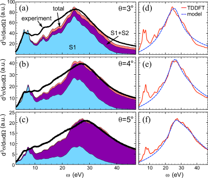
Figure 5: (Color online) TDCS for EELS of C₆₀ at scattering angles $\theta=3^{\circ}$ (a), $\theta=4^{\circ}$ (b), and $\theta=5^{\circ}$ (c). The energy loss $\omega$ is with respect to initial beam energy of $\epsilon_{0}=1050$ eV. Colored curves represent TDDFT calculations resolved in the contribution from S1, S1+S2 and S1+S2+V. The thick curve shows experimental data Verkhovtsev et al. (2012b). (d–f): comparison of full TDDFT and model cross sections.

With the dynamical structure factor being fully characterized, we proceed by computing the TDCS (Eq. (1)). Fig. 5 compares calculated and measured Verkhovtsev et al. (2012b) EELS spectra as a function of the electron scattering angle $\theta$ which fixes the momentum transfer. The magnitudes of the measured spectra shown in Fig. 5 are determined up to an overfall factor. Thus, the theory-experiment comparison in Figs. 5 (b,c) is on an absolute scale. The classification of the plasmon modes accomplished by the NMF analysis allows for plotting mode-resolved TDCS curves. As Figs. 5(a–c) demonstrate, the S1 plasmons play the dominant role for small $\theta$ (which corresponds to the optical limit of small $q$), while the S2 modes becomes increasingly significant for larger $\theta$ (i.e., larger $q$). The larger energy of the S2 with respect to the S1 plasmons leads to the formation of a shoulder (clearly visible for $\theta=4^{\circ}$) and, thus, to the apparent shift of the maximum of the experimental EELS spectrum with growing $\theta$. A similar effect is also observed for the S1 modes due to their dispersion with respect to $\ell$.
Furthermore, the extracted $\omega$-dependencies and the model fluctuation densities can be used to construct an approximate structure factor $S^{\mathrm{model}}(q,\omega)=\sum_{\nu\ell}(2\ell+1)F^{\mathrm{fit}}_{\nu,\ell}(\omega)G^{\mathrm{fit}}_{\nu,\ell}(q)$ that reproduces the TDDFT results around the plasmon resonances in a precise way by construction. Corresponding TDCSs are compared in of Figs. 5(d–f).
An important feature of the structure factor is the $f$-sum rule $\int^{\infty}_{0}\!\mathrm{d}\omega\,\omega S(q,\omega)=Nq^{2}/2$ (number of electrons $N$). Checking for the (plasmon-dominated) $S^{\mathrm{model}}(q,\omega)$ shows the discrepancy for larger $q$; a critical value is reached when $\int^{\infty}_{0}\!\mathrm{d}\omega\,\omega S^{\mathrm{model}}(q,\omega)$ decreases again after quadratic growth. We find $q_{\mathrm{crit}}\sim 1.2$ Å^-1 which is consistent with the estimation above. Hence, $p\mathchar 45\relax h$ excitations become more important for $q>q_{\mathrm{crit}}$ and gradually diminish the plasmon contribution.

In summary, we presented accurate TDDFT calculations for the dynamical structure factor and EELS spectra for C₆₀ molecule underlining the role of higher multipole contributions. Using NMF decomposition allowed to trace the evolution in $q$ and $\omega$ of the symmetric and anti-symmetric surface and volume plasmons. In addition, we characterized and modeled the fluctuation densities (i.e., the ingredients of the response function) and unveiled their multipolar character. These ingredients might, in principle, be accessed selectively by using electron beams carrying a definite angular momentum (electron vortex beams Uchida and Tonomura (2010); Verbeeck et al. (2010)). By measuring the angular momentum of the scattered beam the angular momentum transfer $\Delta\ell$ becomes a control variable which the EELS spectra depends on. Particularly, provided the beam axis coincides with the symmetry axis of spherical system, the plasmonic response upon scattering of such twisted electrons contains multipole contributions for $\ell\geq|\Delta\ell|$ only Note (4). Hence, specific multipoles can be excluded or included by varying $\Delta\ell$.

Furthermore, we discussed the limitation of spherical-shell models in describing the quenching of the volume plasmon and identified the electronic density distribution as a key factor determining its energy. We obtained excellent agreement with experimental results and explained how the different plasmon modes contribute to the spectra.

Appendix A Non-negative matrix factorization

As dictated by the fluctuation-dissipation theorem, the imaginary part of $\delta n_{\ell}(q,\omega)$ for $\omega>0$ is purely negative. Thus, the non-negative matrix factorization (NMF) can be applied to $|\mathrm{Im}[\delta n_{\ell}(q,\omega)]|=-\mathrm{Im}[\delta n_{\ell}(q,\omega)]$ to split

$$\left|\mathrm{Im}\left[\delta n_{\ell}(q,\omega)\right]\right|=\sum^{N}_{\nu=1}F_{\nu,\ell}(\omega)G_{\nu,\ell}(q)\ .$$ (5)

Without imposing any restriction on the number of components ($N$) the expansion (5) is exact and can be paralleled with the singular value decomposition (SVD) of a general (complex or real) matrix $\mathbf{M}$: $\mathbf{M}=\mathbf{U}\mathbf{\Sigma}\mathbf{V}^{*}$. The difference is in the additional requirements of positivity on the vectors forming $\mathbf{U}$ and $\mathbf{V}$. The transition from continuous variables as in eq. (5) to the matrix form is provided by discretizing the $\omega$- and the $q$-points after smooth interpolation.

We select $N=2$ as we expect two dominant surface plasmon modes (S1 and S2). This choice is confirmed by computing the residue norm with respect to the full function $|\mathrm{Im}[\delta n_{\ell}(q,\omega)]|$.

The problem of non-negative matrix factorization can be formulated as a non-convex minimization problem for the residue norm $r=||\mathbf{A}-\mathbf{W}\mathbf{H}||^{2}$. Thus, the solution is not unique and may lead to local minima. Depending on the norm used different algorithms can be formulated. A commonly used method is the multiplicative update of D. Lee and S. Seung Lee and Seung (1999):

$$\mathbf{W}_{ia} \leftarrow \mathbf{W}_{ia}\frac{(\mathbf{A}\mathbf{H}^{T})_{ia}}{(\mathbf{W}\mathbf{H}\mathbf{H}^{T})_{ia}},$$ (6a)

$$\mathbf{H}_{aj} \leftarrow \mathbf{H}_{aj}\frac{(\mathbf{W}^{T}\mathbf{A})_{aj}}{(\mathbf{W}^{T}\mathbf{W}\mathbf{H})_{aj}},$$ (6b)

where $i$ indexes the energy points and $j$ numbers the time points. The method starts with some suitable guess for matrices $\mathbf{W}$ and $\mathbf{H}$. Additionally, the vectors forming $\mathbf{W}$ are normalized each step:

$$\mathbf{W}_{ia}\leftarrow\frac{\mathbf{W}_{ia}}{\|\mathbf{W}_{a}\|}.$$

Upon these prescriptions (6) the Euclidean distance $r$ monotonously decreases until the stationary point (local minimum) has been reached. We initialized the vector $\mathbf{W}_{1}$ ($\mathbf{W}_{2}$) with cuts of $|\mathrm{Im}[\delta n_{\ell m}(q,\omega)]|$ along $q$ direction at $\omega=20$ eV ($\omega=40$ eV), while $\mathbf{H}_{1}$ ($\mathbf{H}_{2}$) is constructed by cuts at $q=0.5$ Å^-1 ($q=1.0$ Å^-1). We found that typically 1000 iterations yield well converged results.

The functions $F_{\nu,\ell}(\omega)$ and $G_{\nu,\ell}(q)$ is then obtained from interpolating the data from $\mathbf{H}_{\nu}$ and $\mathbf{W}_{\nu}$, respectively. We normalize the frequency spectra such that fitting by $F^{\mathrm{fit}}_{\nu,\ell}(\omega)=\mathrm{Im}[2\omega_{\nu,\ell}/((\omega+\mathrm{i}\Gamma_{\nu,\ell})^{2}-\omega^{2}_{\nu,\ell})]$ (as explained in the main text) can be performed without any additional prefactor. $G_{\nu,\ell}(q)$ is normalized accordingly. This normalization procedure is consistent with the Lehmann representation.

Appendix B Semi-classical calculations

In order to eludicate the behavior of the volume plasmons, semi-classical calculations provide some insight. The starting point is the Dyson equation for the density-density response function in random-phase approximation (RPA):

$$\begin{split}\chi(\mathbf{r},\mathbf{r}^{\prime};z)=\chi^{(0)}(\mathbf{r},\mathbf{r}^{\prime};z)+&\int\!\mathrm{d}\mathbf{r}_{1}\int\!\mathrm{d}\mathbf{r}_{2}\,\chi^{(0)}(\mathbf{r},\mathbf{r}_{1};z)\\ &\times v(\mathbf{r}_{1}-\mathbf{r}_{2})\chi(\mathbf{r}_{2},\mathbf{r}^{\prime};z)\ .\end{split}$$ (7)

We drop the superscript R and consider general complex argument $z$ here. In SCA, the non-interacting reference response function $\chi^{(0)}(\mathbf{r},\mathbf{r}^{\prime};z)$ can be expressed in terms of ground-state density $n_{0}(\mathbf{r})$ ($=n_{0}(r)$ as we assume spherical symmetry here) only. The subsequent derivations and the solution scheme for eq. (7) are detailed in the Supplementary Material Note (5). The amount of spill-out density can be adjusted by varying the smearing parameter $\Delta r$ in the model density

$$\begin{split}n_{0}(r)&=N_{0}\big{[}\theta_{\Delta r}(r-R_{1})-\theta_{\Delta r}(r-R_{2})\big{]}\ ,\\ \theta_{\Delta r}(r)&=\frac{1}{1+\exp[-r/\Delta r]}\ ,\end{split}$$ (8)

where $R_{1}=R_{0}-\Delta R/2$, $R_{2}=R_{0}+\Delta R/2$ are the inner and outer radii ($R_{0}=6.5$ a.u.), while the normalization $N_{0}$ ensures the correct total valence charge. $\Delta R$ is fixed to keep the mean density constant. The scenario $\Delta r\rightarrow 0$ corresponds to a box-like density profile with sharp boundaries, while $\Delta r=0.5$ a.u. is a good approximation to the spherically-averaged DFT density. Once eq. (7) is solved for certain $\Delta r$, the $(\ell=0)$ contribution to the structure factor, $\mathrm{Im}[\delta n_{0}(q,z=\omega+\mathrm{i}\Gamma)]$ ($\Gamma=0.1$ a.u. is a broading parameter) can be computed. Applying the NMF technique allows again for separating the V1 and V2 modes. We find the position of V1 similar to the TDDFT results, while the behavior of V2 is very sensititve to $\Delta r$. While very pronounced for $\Delta r=0.5$ a.u., the relative strength of the V2 peak vanishes for $\Delta r\rightarrow 0$. More details and graphs of volume plasmon spectra can be found in the Supplementary Material.