Controlling Anderson localization in disordered heterostrctures with Lévy-type distribution

Abstract

In this paper, we propose a disordered heterostructure in which the distribution of refractive index of one of its constituents follows a Lévy-type distribution characterized by the exponent $\alpha$. For the normal and oblique incidences, the effect of $\alpha$ variation on the localization length is investigated in different frequency ranges. As a result, the controllability of Anderson localization can be achieved by changing the exponent $\alpha$ in the disordered structure having heavy tailed distribution.

I Introduction

In the past few decades, localization of waves in disordered structures known as Anderson localization has attracted growing attention, in various fields of physics. Starting from early studies of the localization of electronic wave functions in disordered crystals anderson58 , it is believed that the localized states appear in a wide variety of classical and quantum materials. The possible occurrence of Anderson localization for electrons in disordered solids Evers2008 , ultrasound and acoustic waves Strybulevych , the transport of light Wiersma1997 ; Maret2006 , microwave Dalichaouch , matter waves Billy ; Roati and cold atoms Kondov are just a few examples among many others.

All these disordered systems are typically composed of regions with very different kinds of the spatial distribution of disorder. The question is what one would expect for effects of the distribution of disorder on controlling the localization properties. This interesting question has been basis of numerous theoretical and experimental studies Moura ; Izrailev ; Iomin ; Falceto ; Costa ; Fernandez-Marin2012 ; Fernandez-Marin2013 ; Fernandez-Marin2014 ; zakeri .

More recently, some engineered tunable random mediums have been assembled in the lab that follows the Lévy type distribution Fernandez-Marin2012 ; Fernandez-Marin2014 ; zakeri . Lévy processes have a power-law distribution $p(x)\sim x^{-(1+\alpha)}$, where $\alpha$ is the so called Lévy exponent Uchaikin . Power law distributions have been appeared in different physical phenomena such as spectral fluctuation in random lasers Lepro2007 ; Sharma2006 , superdiffusive transport of light across glass microspheres whose diameters have levy distribution Barthelemy , quantum coherent transport of electrons in one- dimensional ($1$D) disordered wires with Lévy-type distribution Falceto .

Recently, Fernandez-Marin et al. have investigated numerically how transmission of electromagnetic waves varies with the system size in a $1$D random system in which the layer thicknesses follow a Lévy-type distribution with the exponent $\alpha$ Fernandez-Marin2013 . They demonstrated that $\langle-\ln T\rangle\propto L^{\alpha}$ for $0<\alpha<1$ , whereas $\langle-\ln T\rangle$ is proportional to the system size $L$ for $1<\alpha<2$ Fernandez-Marin2013 . Furthermore, Fernandez-Marın et al. have experimentally studied the microwave electromagnetic wave transmission through a waveguide composed of dielectric slabs where spacing between them follows a distribution with a power-law tail ($\alpha$-stable Lévy distribution) Fernandez-Marin2014 . They observed an anomalous localization for the case $0<\alpha<1$ in which transmission $\langle T\rangle$ decays with length of waveguide as $L^{-\alpha}$ while in the case of standard localization $\langle T\rangle\propto\exp(-L/\xi)$, $\xi$ being the localization length Fernandez-Marin2014 .

More recently, Zakeri et al. have investigated Anderson localization of the classical lattice waves in a chain with mass impurities distributed randomly through a power-law relation $s^{-(1+\alpha)}$ where $s$ is the distance between two successive Impurities zakeri . For this 1D harmonic disordered lattice of $n$-sites with random masses $m_{n}$, they have indicated that in the small frequencies for $1<\alpha<2$, the localization length behaves as $\xi(\omega)\sim\omega^{-\alpha}$.

In this paper, we propose a 1D disordered multilayered structure in which the random refractive index of one of its constituents follows a probability density function with a power-law tail with exponent $\alpha$ (Lévy-type distribution). The propagation of an obliquely incident electromagnetic wave through the structure is studied using the transfer matrix method. The effects of variation of the exponent $\alpha$ on the localization length and Anderson localization are investigated in different frequency ranges. It is shown that the localization length decreases with decreasing $\alpha$ for both $1<\alpha<2$ and $0<\alpha<1$ at intermediate and large frequencies. Furthermore, at small frequencies the localization length depends on values of $\alpha$. In this structure, the localization length can be also affected by the incident angle.

The paper is organized as follows: in Sec. II we introduce the notation. The numerical results are discussed in Sec. III. Finally, we draw our conclusions in Sec. IV.

II Definitions and settings

The disordered multilayered structure that we shall to study composed of an alternating sequence of layers of $A$ and $B$ having thickness of $d_{A}$ an $d_{B}$. Fig. (1) displays a scheme of the proposed structure.

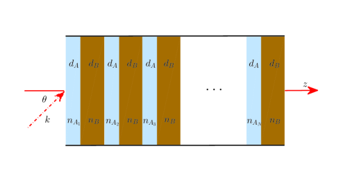
Figure 1: (Color online)Sketch of a heterostructure of length $L$ with $N$ layers with the fixed thickness $d_{A(B)}$. The refractive index $n_{B}$ is fixed and the distribution of the $n_{A}$s follows a Lévy-type distribution.

It is assumed that the layers $B$ have the same refractive index $n_{B}$ and the same width of $d_{B}$, while layers $A$ have the same thickness of $d_{A}$ and random refractive indices $n_{Aj}$($j=1,2,\dots,N$). The number of layers in the structure is taken to be $2N$ and the $z$-axis is directed across the layers.

Here we consider $n_{Aj}\propto\sqrt{\mid\delta_{j}\mid}$, where $\delta_{j}$ are independent identically distributed random variables with standard symmetric $\alpha$-stable distribution. The procedure of computer simulating realizations of the random variables $\delta_{j}$ is the following chambers1976method ; weron1996chambers :

$$\delta_{j}=\frac{\sin\left(\alpha V\right)}{\left[\cos\left(V\right)\right]^{1/\alpha}}\left(\frac{\cos\left(V-\alpha V\right)}{W}\right)^{(1-\alpha)/\alpha}$$ (1)

where random variable $W$ has exponential distribution with mean $1$ and $V$ is uniformly distributed on $\left(-\pi/2,\pi/2\right)$. The algorithm introduced in Eq. (1) allows us to generate a sequence of random numbers with $\alpha$-stable distribution for the whole range of parameter $0<\alpha\leqslant 2$. The main feature of a $\alpha$-stable Lévy density distribution $P(\delta)$ is the power-law, decay of its tail which behaves as: $P(\delta)\sim 1/\delta^{1+\alpha}$.

We choose random numbers $\delta_{j}$ which their absolute values are in the range $5<\mid\delta_{j}\mid<100$. The refractive index of layer $A$ is taken to be $n_{Aj}=\sqrt{\mid\delta_{j}\mid/5}$.

The transfer matrix formalism is used to compute the localization length of the structure. We consider a monochromatic electromagnetic wave obliquely incident from left into the random structure. In Fig. (1), $k$ and $\theta$ denote the wave vector and incident angle, respectively. The wave vector $k$ is taken to be in $xz$-plane. The electric and magnetic fields at incident and exit ends of the structure can be related by the product of transfer matrix of different layers included in the heterostructure as:

$$\begin{pmatrix}E_{0}\\ H_{0}\end{pmatrix}=M_{1}M_{2}M_{3}\dots M_{2N}\begin{pmatrix}E^{2N+1}\\ H^{2N+1}\end{pmatrix}=M\begin{pmatrix}E^{2N+1}\\ H^{2N+1}\end{pmatrix},$$ (2)

where $M$ is the total transfer matrix of the system and $M_{j}$($j=1,2,\dots,2N$) is the transfer matrix of the $j^{\textrm{th}}$ dielectric layer which is defined as:

$$M_{j}=\begin{pmatrix}\cos\left(k_{zj}d_{j}\right)&-\frac{i}{\eta_{j}}\sin\left(k_{zj}d_{j}\right)\\ -i\sin\left(k_{zj}d_{j}\right)&\cos\left(k_{zj}d_{j}\right)\par\end{pmatrix},$$ (3)

here $\eta^{2}_{j}=(\epsilon_{0}/\mu_{0})\epsilon_{j}/\cos^{2}\theta_{j}$ for TM case and $\eta^{2}_{j}=(\epsilon_{0}/\mu_{0})\epsilon_{j}\cos^{2}\theta_{j}$ for TE case, $k_{zj}=k_{j}\cos\theta_{j}$ denotes the $z$ component of the wave vector in dielectric layers, and $d_{j}$ is the thickness of different dielectric layers. For a plane wave strikes from left into the disordered structure, the transmission coefficient $t(\omega)$ is expressed in terms of the matrix element of $M$ as follows:

$$t(\omega)=\frac{2\eta_{0}}{M_{11}\eta_{0}+M_{12}\eta_{0}\eta_{N+1}+M_{21}+M_{22}\eta_{N+1}}.$$ (4)

The corresponding transmittance of the structure at frequency $\omega$ is:

$$T(\omega)=\frac{\eta_{N+1}}{\eta_{0}}\mid t(\omega)\mid^{2}.$$ (5)

To study the localization behavior in the $1$D random system, it is required to evaluate the localization length. Since the transmittance in the localized regime exponentially decays with the system length $L$, the localization length $\xi$ can be numerically calculated as

$$\xi(\omega)=-\lim_{L\rightarrow\infty}\frac{2L}{\ln\left(T(\omega,L)\right)}.$$ (6)

For a sufficiently long random-layered system, $\xi$ obtained from the above equation is a nonrandom number due to self-averaging. However, for a system with a finite size, the localization length can be obtained by ensemble averaging of the transmittance $T$ over many realizations. This means that we introduce the localization length of a finite random configuration as

$$\xi(\omega)=-\frac{2L}{\langle\ln\left(T(\omega,L)\right)\rangle}.$$ (7)

where $\langle\dots\rangle$ stands for the ensemble averaging. The values of those parameters used in the following calculations are $d_{A}=20\textrm{mm}$, $d_{B}=40\textrm{mm}$, $n_{B}=1$ and $N=500$. In the next section, we will discuss our numerical findings.

III Results and discussion

We first study the case at which the plane wave is normally incident into the random structure. It is assumed the frequency of the incident wave is in the range $3\times 10^{8}\textrm{(rad/s)}<\omega<3\times 10^{10}\textrm{(rad/s)}$. In order to understand how localization length can be affected by the variation of $\alpha$ values, in Fig. (2), we plot the localization length in units of the system length (normalized localization length) as a function of frequency $\omega$ for different values of $\alpha$. To obtain localization length, $2\times 10^{4}$ different random realizations with the same $\alpha$ values and the same number of layers are considered.

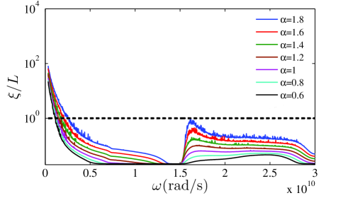
Figure 2: (Color online) Localization lengths in units of the system size for normal incidence in the frequency range $3\times 10^{8}\textrm{(rad/s)}<\omega<3\times 10^{10}\textrm{(rad/s)}$ for different $\alpha$ values.

As shown in Fig. (2), the localization length decreases with decreasing the exponent $\alpha$ at some frequency ranges. For frequencies at which normalized localization length of the wave is lower than one, the system is in the localized regime. When $\alpha$ decreases from $1.8$ to $0.6$, the minimum frequency at which localization occurs shifts toward lower frequencies. Our numerical results confirm the self-averaging of the localization length. That is the localization length obtained from Eq. (7) does not significantly differ from the localization length of a single realization with large number of layers. Furthermore, increasing the number of random realizations from $2\times 10^{4}$ does not lead to any considerable change in localization length values.

To determine whether or not this dependence of localization length on the $\alpha$ values is observed in the case of oblique incidence, we display the normalized localization length versus frequency for $\theta=15^{\circ}$ and $\theta=30^{\circ}$ in Fig. (3).

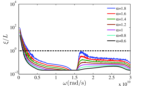
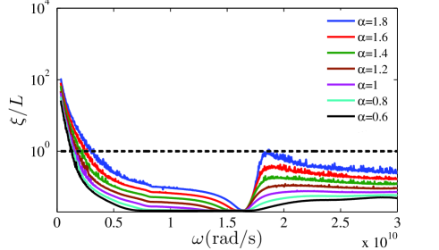
Figure 3: (Color online) Localization lengths in units of the system size for oblique incidence $\theta=15^{\circ}$ (top) and $\theta=30^{\circ}$ (bottom) in the frequency range $3\times 10^{8}\textrm{(rad/s)}<\omega<3\times 10^{10}\textrm{(rad/s)}$ for different $\alpha$ values.

The corresponding frequency range is the same as that in Fig. (2). It is clearly seen in Fig. (3) that for oblique incidence the localization length decreases when the exponent $\alpha$ decreases from $1.8$ to $0.6$. To better understand the effect of incident angle on the localization length, in Fig. (5) we show the normalized localization length versus $\alpha$ for different incident angles $\theta=0$, $15^{\circ}$ and $30^{\circ}$ with the same $\alpha=1.8$.

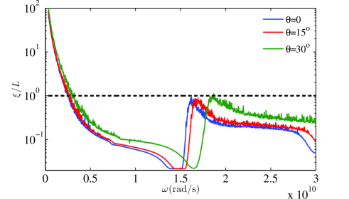
Figure 4: (Color online)Localization lengths in units of the system size for different incident angles $\theta=0$, $15^{\circ}$ and $30^{\circ}$ in the frequency range $3\times 10^{8}\textrm{(rad/s)}<\omega<3\times 10^{10}\textrm{(rad/s)}$ with the same $\alpha$ values.

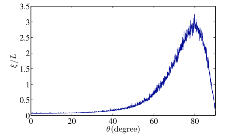
Figure 5: (Color online)Localization lengths in units of the system size versus incident angle $\theta$ for $\alpha=0.6$ and $\omega=2\times 10^{9}\textrm{(rad/s)}$.

One can see that the localization length increases with incident angle at some frequency regions. Furthermore, the dip in localization length moves to higher frequencies with increasing incident angle. Therefore, our calculated results indicate that the localization length depends on the incident angle as well as the exponent $\alpha$.

It is well known that for TM polarized waves propagating in a 1D random structure the localization length takes a large maximum value at some critical angles which are called generalized Brewster angles brewster1 . It has been demonstrated that generalized Brewster angle increases from $0^{\circ}$ to $90^{\circ}$ with increasing the disorder-averaged refractive index brewster1 . The localization length for a weak disorder diverges in the vicinity oh $\theta=45^{\circ}$ when the average of refractive index is equal to 1 brewster1 ; brewster2 . This phenomenon is known as Brewster anomalies and the corresponding angle is called the Brewster angle brewster1 ; brewster2 . In Fig. (5), we display the localization length versus incident angle for $\alpha=0.6$ and $\omega=2\times 10^{9}\textrm{(rad/s)}$. One can see that the generalized Brewster angle is about $80^{\circ}$ at which the localization length is significantly enhanced over its value at the normal incidence ($\theta=0^{\circ}$). Moreover, for incident angle in the range $68^{\circ}<\theta<88^{\circ}$, the system is in the extended regime, while at other incident angle the system is in the localized regime. The effects of $\alpha$ variation on the generalized Brewster angle and Brewster anomalies are under investigation and their results will be reported in the near future.

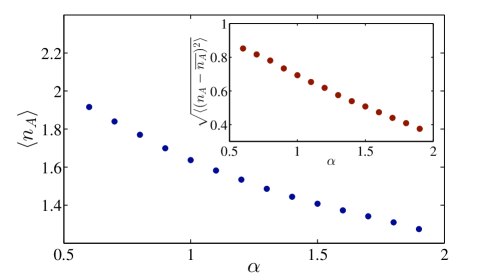
Figure 6: (Color online) Mean and variance (inset) values of refractive index $n_{A}$ as a function of the exponent $\alpha$.

To understand the physical reason for the behavior of localization length with $\alpha$, in Fig. (6), we plot the mean value of refractive index versus $\alpha$. As shown in Fig. (6), the average value of refractive index increases with increasing $\alpha$. As a result, increases of $\alpha$ leads to the decreasing the refractive index contrast between the layers of disordered system. This effect causes the scattering strength to decrease. Hence, we expect that the localization length decreases with increasing $\alpha$. In addition, the Fig. (6) represents the variance of refractive index versus $\alpha$. One can see that the variance of refractive index increases with decreasing $\alpha$. Therefore, the randomness strength increases with decreasing $\alpha$. This effect also results in the enhancement of localization with decreasing $\alpha$.

Now, we shall to study how heavy-tail distribution of random refractive index $n_{A}$ affects the normalized localization length in the frequency range $2.5\times 10^{12}\textrm{(rad/s)}<\omega<3\times 10^{12}\textrm{(rad/s)}$. Fig. (7) shows the corresponding results for different values of $\alpha=1.8$, $1.4$, $1.0$ and $0.6$.

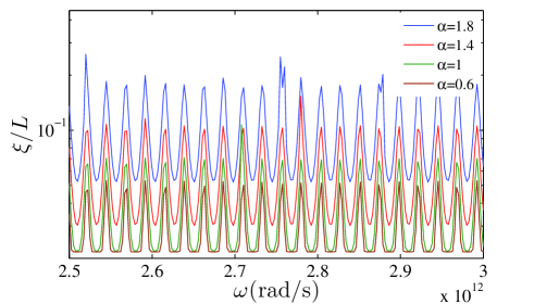
Figure 7: (Color online) Localization lengths in units of the system size for normal incidence in the frequency range $2.5\times 10^{12}\textrm{(rad/s)}<\omega<3\times 3^{12}\textrm{(rad/s)}$ for different $\alpha$ values.

It is clearly seen that the normalized localization length shows an oscillatory behavior in this frequency range for different $\alpha$ values. Moreover, for all frequencies in this frequency range and for all $\alpha$ values, we have a localized mode whose localization length decreases with decreasing $\alpha$. As a result, decreasing $\alpha$ value improves the localization. This effect is attributed to the enhancement of mean value and variance of refractive index with decreasing $\alpha$.

Next, we consider the effect of $\alpha$ variation on the normalized localization length for longer wavelengths. The normalized localization lengths versus $\omega$ in frequency range $3\times 10^{6}\textrm{(rad/s)}<\omega<2.5\times 10^{8}\textrm{(rad/s)}$ are displayed in Fig. (8) for different values of $\alpha=1.8$, $1.4$, $1.0$ and $0.6$.

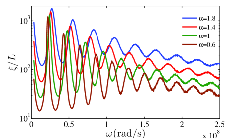
Figure 8: (Color online) Localization lengths in units of the system size for normal incidence in the frequency range $3\times 10^{6}\textrm{(rad/s)}<\omega<2.5\times 10^{8}\textrm{(rad/s)}$ for different $\alpha$ values.

As shown in this figure, the localization length indicates an oscillatory behavior where their peak values increases with lowering the frequency for all $\alpha$ values. For all wavelengths, the system is in the extended regime. With decreasing the $\alpha$ values, the peaks of normalized localization length shift to lower frequencies, while the peak values decreases.

Consequently, our results demonstrate that if the distribution of the random layer in a $1$D disordered system follows the $\alpha$-stable Lévy distribution, the localization length can be manipulated with the exponent $\alpha$. Due to the random nature of Anderson localization, the control of this phenomenon in a regular manner is of great importance and has potential applications.

IV Conclusion

We have studied the localization of an electromagnetic wave normally and obliquely incident into a $1$D disordered structure where the refractive index of one its constituents is fixed while that of the other constituents is a random number drawn from a Lévy-type distribution with exponent $\alpha$. It has been demonstrated that for normal incidence the localization behavior in this structure can be manipulated in a regular manner by changing the value of $\alpha$. When $\alpha$ decreases, the localization length of the waves decreases in the frequency range $3\times 10^{8}\textrm{(rad/s)}<\omega<1.9\times 10^{10}\textrm{(rad/s)}$ decreases. This effect is due to the increase of mean and variance of refractive index with decrease of $\alpha$. Moreover, the minimum frequency at which localization appears shifts to lower frequencies with decreasing $\alpha$. Localization length shows the same trend with variation of $\alpha$ for oblique incidence. It has been also investigated how the localization length can be affected by $\alpha$ variation in the lower and higher frequency ranges. In the frequency range $2.5\times 10^{12}\textrm{(rad/s)}<\omega<3\times 10^{12}\textrm{(rad/s)}$, the system is in the localized regime and the localization length indicate an oscillatory behavior with approximately fixed amplitudes. Decrease of $\alpha$ in this frequency range also gives rise to the enhancement of localization. In the frequency range $3\times 10^{6}\textrm{(rad/s)}<\omega<2.5\times 10^{8}\textrm{(rad/s)}$. it is found the system is in the extended regime and the localization length exhibits an oscillatory behavior with increasing amplitude whose value decreases with decreasing $\alpha$. Furthermore, reduction of $\alpha$ causes the peaks of localization length to shift toward lower frequencies. Consequently, in disordered media, employing the $\alpha$-stable Lévy distribution provides a way to easily control the localization phenomenon.

References

- (1) P. W. Anderson, Phys. Rev. 109, 1492 (1958).
- (2) F. Evers and A.D. Mirlin, Rev. Mod. Phys. 80, 1355 (2008).
- (3) H. Hu, A. Strybulevych, J.H. Page, S.E. Skipetrov, and B.A. van Tiggelen, Nature Phys. 4, 945 (2008).
- (4) D. S. Wiersma, P. Bartolini, A. Lagendijk, R. Righini, Nature 390, 671 (1997).
- (5) M. Storzer, P. Gross, C. M. Aegerter, G. Maret, Phys. Rev. Lett. 96, 063904 (2006).
- (6) R. Dalichaouch, J.P. Armstrong, S. Schultz, P.M. Platzman and S.L. McCall, Nature 354, 53-55 (1991).
- (7) J. Billy, et al., Nature 453, 891 (2008).
- (8) G. Roati, et al., Nature 453, 895 (2008).
- (9) S. S. Kondov, W. R. McGehee, J. J. Zirbel, and B. DeMarco, Science 334, 66 (2011).
- (10) Francisco A. B. F. de Moura and Marcelo L. Lyra,Phys. Rev. Lett. 81, 3735 (1998)
- (11) F. M. Izrailev and A. A. Krokhin Phys. Rev. Lett. 82, 4062 (1999)
- (12) A. Iomin, Phys. Rev. E 79, 062102 (2009).
- (13) F. Falceto and V. A. Gopar, EPL 92 (2010).
- (14) A E B Costa and F A B F de Moura 2011 J. Phys.: Condens. Matter 23 065101
- (15) A.A. Fernández-Marín, J. A. Méndez-Bermúdez and V. A. Gopar, Phys. Rev. A 85, 035803 (2012).
- (16) A.A. Fernández-Marín, J. A. Méndez-Bermúdez and V. A. Gopar, Phys. Rev. A 87, 039908 (2013).
- (17) A.A. Fernández-Marín, J. A. Méndez-Bermúdez, J. Carbonell, F. Cervera, J. Sánchez-Dehesa and V. A. Gopar, Phys. Rev. Lett. 113, 233901 (2014).
- (18) S. S. Zakeri, S. Lepri, and D. S. Wiersma, Phys. Rev. E 91, 032112 (2015).
- (19) Uchaikin V. V. and V. M. Zolotarev V. M., Chance and Stability: Stable Distributions and their Applications (VSP, Utrecht, Netherlands, and references therein) 1999
- (20) Lepri, S., Cavalieri, S., Oppo, G.-L. and Wiersma, D. S. Statistical regimes of random laser fluctuations. Phys. Rev. A 75, 063820 (2007).
- (21) Sharma, D., Ramachandran, H. and Kumar, N. Levy statistical fluctuations from a random amplifying medium. Fluct. Noise Lett. 6, 95–101 (2006).
- (22) Pierre Barthelemy, Jacopo Bertolotti and Diederik S. Wiersma, Nature, 453 (2008) 495.
- (23) F. Falceto and V. A. Gopar, Europhys. Lett. 92, 57014 (2010).
- (24) J. M. Chambers,L. M. Colin and B. W. Stuck, Journal of the american statistical association 71.354 (1976): 340-344.
- (25) R. Weron, Statistics and probability letters 28.2 (1996): 165-171.
- (26) K. J. Lee, K. Kim, Optics Express, 19, 20817- 20826 (2011)
- (27) J. E. Sipe, P. Sheng, B. S. White, M. H. Cohen, Phys. Rev. Lett. 60, 108-111 (1988)