Evidential relational clustering using medoids

Abstract

In real clustering applications, proximity data, in which only pairwise similarities or dissimilarities are known, is more general than object data, in which each pattern is described explicitly by a list of attributes. Medoid-based clustering algorithms, which assume the prototypes of classes are objects, are of great value for partitioning relational data sets. In this paper a new prototype-based clustering method, named Evidential $C$-Medoids (ECMdd), which is an extension of Fuzzy $C$-Medoids (FCMdd) on the theoretical framework of belief functions is proposed. In ECMdd, medoids are utilized as the prototypes to represent the detected classes, including specific classes and imprecise classes. Specific classes are for the data which are distinctly far from the prototypes of other classes, while imprecise classes accept the objects that may be close to the prototypes of more than one class. This soft decision mechanism could make the clustering results more cautious and reduce the misclassification rates. Experiments in synthetic and real data sets are used to illustrate the performance of ECMdd. The results show that ECMdd could capture well the uncertainty in the internal data structure. Moreover, it is more robust to the initializations compared with FCMdd.

I Introduction

Clustering is a useful technique to detect the underlying cluster structure of the data set. The goal of clustering is to partition a set of objects $X=\{x_{1},x_{2},\cdots,x_{n}\}$ into $c$ small subgroups $\Omega=\{\omega_{1},\omega_{2},\cdots,\omega_{c}\}$ based on a well defined measure of similarities between patterns. To measure the similarities (or dissimilarities), the objects are described by either object data or relational data. Object data are described explicitly by a feature vector, while relational data arise from the pairwise similarities or dissimilarities. Among the existing approaches to clustering, the objective function-driven or prototype-based clustering such as $C$-Means (CM) and Fuzzy $C$-Means (FCM) is one of the most widely applied paradigms in statistical pattern recognition. These methods are based on a fundamentally very simple, but nevertheless very effective idea, namely to describe the data under consideration by a set of prototypes. They capture the characteristics of the data distribution (like location, size, and shape), and classify the data set based on the similarities (or dissimilarities) of the objects to their prototypes.

The above mentioned clustering algorithms, CM and FCM are for object data. The prototype of each class in these methods is the center of gravity of all the included patterns. But for relational data set, it is difficult to determine the centers of objects. In this case, one of the objects which is most similar to the center could be the most rational choice to be setting as the prototype. This is the idea of clustering using medoids. Some clustering methods, such as Partitioning Around Medoids (PAM) [1] and Fuzzy $C$-Medoids (FCMdd) [2], produce hard and soft clusters where each of them is represented by a representative object (medoid).

Belief functions have already been applied in many fields, such as data classification [3], data clustering [4, 5], social network analysis [6, 7] and statistical estimation [8, 9]. Evidential $C$-means (ECM) [4] is a newly proposed clustering method to get credal partitions for object data. The credal partition is a general extension of the crisp (hard) and fuzzy ones and it allows the object to belong to not only single clusters, but also any subsets of the set of clusters $\Omega=\{\omega_{1},\cdots,\omega_{c}\}$ by allocating a mass of belief for each object in $X$ over the power set $2^{\Omega}$. The additional flexibility brought by the power set provides more refined partitioning results than those by the other techniques allowing us to gain a deeper insight into the data [4]. In this paper, we introduce an extension of FCMdd on the framework of belief functions. The evidential clustering algorithm for relational data sets, named ECMdd, using a medoid which is assumed to belong to the original data set to represent a class are proposed to produce the optimal credal partition. The experimental results show the effectiveness of the methods and illustrate the advantages of credal partitions.

The rest of this paper is organized as follows. In Section II, some basic knowledge and the rationale of our method are briefly introduced. In Section III the proposed ECMdd clustering approach is presented in detail. In Section IV we test ECMdd using various data sets and compare it with several other classical methods. Finally, we conclude and present some perspectives in Section V.

II Background

II-A Theory of belief functions

Let $\Omega=\{\omega_{1},\omega_{2},\ldots,\omega_{c}\}$ be the finite domain of $X$, called the discernment frame. The belief functions are defined on the power set $2^{\Omega}=\{A:A\subseteq\Omega\}$.

The function $m:2^{\Omega}\rightarrow[0,1]$ is said to be the Basic Belief Assignment (bba) on $2^{\Omega}$, if it satisfies:

$$\sum_{A\subseteq\Omega}m(A)=1.$$ (1)

Every $A\in 2^{\Omega}$ such that $m(A)>0$ is called a focal element. The credibility and plausibility functions are defined as in Eq.$~{}\eqref{bel}$ and Eq.$~{}\eqref{pl}$.

$$Bel\text{(}A\text{)}=\sum_{B\subseteq A,B\neq\emptyset}m\text{(}B\text{)}~{}~{}\forall A\subseteq\Omega,$$ (2)

$$Pl\text{(}A\text{)}=\sum_{B\cap A\neq\emptyset}m\text{(}B\text{)},~{}~{}\forall A\subseteq\Omega.$$ (3)

Each quantity $Bel(A)$ measures the total support given to $A$, while $Pl(A)$ represents potential amount of support to $A$.

A belief function on the credal level can be transformed into a probability function by Smets method [10]. In this algorithm, each mass of belief $m(A)$ is equally distributed among the elements of $A$. This leads to the concept of pignistic probability, $BetP$, defined by

$$BetP(\omega_{i})=\sum_{\omega_{i}\in A\subseteq\Omega}\frac{m(A)}{|A|(1-m(\emptyset))},$$ (4)

where $|A|$ is the number of elements of $\Omega$ in $A$.

II-B Evidential $c$-means

Evidential $c$-means [4] is a direct generalization of FCM in the framework of belief functions based on the concept of credal partitions. The credal partition takes advantage of imprecise (meta) classes to express partial knowledge of class memberships. In ECM, the evidential membership of an object $x_{i}$ is represented by a bba $m_{i}=\left(m_{i}\left(A_{k}\right):A_{k}\subseteq\Omega\right)$ $(i=1,2,\cdots,n)$ over the given frame of discernment $\Omega$. The set $\left\{A_{k}\mid A_{k}\subseteq\Omega,k=1,2,\cdots,2^{c}\right\}$ contains all the focal elements. The optimal credal partition is obtained by minimizing the following objective function:

$$J_{\mathrm{ECM}}=\sum\limits_{i=1}^{n}\sum\limits_{A_{k}\subseteq\Omega,A_{k}\neq\emptyset}|A_{k}|^{\alpha}m_{i}(A_{k})^{\beta}d_{ik}^{2}+\sum\limits_{i=1}^{n}\delta^{2}m_{i}(\emptyset)^{\beta}$$ (5)

constrained on

$$\sum\limits_{A_{k}\subseteq\Omega,A_{k}\neq\emptyset}m_{i}(A_{k})+m_{i}(\emptyset)=1,$$ (6)

and

$$m_{i}\left(A_{k}\right)\geq 0,~{}~{}m_{i}\left(\emptyset\right)\geq 0,$$ (7)

where $m_{i}(A_{k})\triangleq m_{ik}$ is the bba of $x_{i}$ given to the nonempty set $A_{k}$, while $m_{i}(\emptyset)\triangleq m_{i\emptyset}$ is the bba of $x_{i}$ assigned to the empty set. Parameter $\alpha$ is a tuning parameter allowing to control the degree of penalization for subsets with high cardinality, parameter $\beta$ is a weighting exponent and $\delta$ is an adjustable threshold for detecting the outliers. Here $d_{ik}$ denotes the distance (generally Euclidean distance) between $x_{i}$ and the barycenter (i.e. prototype, denoted by $\overline{v}_{k}$) associated with $A_{k}$:

$$d_{ik}^{2}=\|x_{i}-\overline{v}_{k}\|^{2},$$ (8)

where $\overline{v}_{k}$ is defined mathematically by

$$\overline{v}_{k}=\frac{1}{|A_{k}|}\sum_{h=1}^{c}s_{hk}v_{h},~{}~{}\text{with}~{}~{}s_{hk}=\begin{cases}1&\text{if}~{}~{}\omega_{h}\in A_{k}\\ 0&\text{else}\end{cases}.$$ (9)

The notation $v_{h}$ is the geometrical center of points in cluster $h$. The update process with Euclidean distance is given by the following two alternating steps.

• Assignment update, $\forall i,~{}\forall k/A_{k}\subseteq\Omega,A_{k}\neq\emptyset$:

  $$m_{ik}=\frac{|A_{k}|^{-\alpha/(\beta-1)}{d_{ik}^{-2/(\beta-1)}}}{\sum\limits_{A_{h}\neq\emptyset}|A_{h}|^{-\alpha/(\beta-1)}{d_{ih}^{-2/(\beta-1)}}+\delta^{-2/(\beta-1)}},$$ (10)

  and for $A_{k}=\emptyset$

  $$m_{i\emptyset}=1-\sum_{A_{k}\neq\emptyset}m_{ik},~{}~{}\forall i=1,2,\cdots,n.$$ (11)

• Prototype update: The prototypes (centers) of the classes are given by the rows of the matrix $v_{c\times p}$, which is the solution of the following linear system:

  $$\bm{HV}=\bm{B},$$ (12)

  where $\bm{H}$ is a matrix of size $(c\times c)$ given by

  $$\bm{H}_{lk}=\sum_{i}\sum_{A_{k}\supseteqq\{\omega_{k},\omega_{l}\}}|A_{k}|^{\alpha-2}m_{ik}^{\beta},$$ (13)

  and $\bm{B}$ is a matrix of size $(c\times p)$ defined by

  $$\bm{B}_{lq}=\sum_{i=1}^{n}x_{iq}\sum_{A_{k}\ni\omega_{l}}|A_{k}|^{\alpha-1}m_{ik}^{\beta}.$$ (14)

II-C Fuzzy $c$-medoids

Fuzzy $C$-Medoids (FCMdd) is a variation of classical $c$-means clustering designed for relational data [2]. Let $\bm{X}=\left\{x_{i}\mid i=1,2,\cdots,n\right\}$ be the set of $n$ objects and $\tau(x_{i},x_{j})\triangleq\tau_{ij}$ denote the dissimilarity between objects $x_{i}$ and $x_{j}$. Each object may or may not be represented by a feature vector. Let $\bm{V}=\{v_{1},v_{2},\cdots,v_{c}\}$, $v_{i}\in\bm{X}$ represent a subset of $\bm{X}$. The objective function of FCMdd is given as

$$J_{\text{FCMdd}}=\sum_{i=1}^{n}\sum_{j=1}^{c}u_{ij}^{\beta}\tau(x_{i},v_{j})$$ (15)

subject to

$$\sum_{j=1}^{c}u_{ij}=1,i=1,2,\cdots,n,$$ (16)

and

$$u_{ij}\geq 0,i=1,2,\cdots,n,~{}~{}j=1,2,\cdots,c.$$ (17)

In fact, the objective function of FCMdd is similar to that of FCM. The main difference lies in that the prototype of a class in FCMdd is defined as the medoid, i.e., one of the object in the original data set, instead of the centroid (the average point in a continues space) for FCM. FCMdd is preformed by the following alternating update steps:

• Assignment update:

  $$u_{ij}=\frac{\tau_{ij}^{-1/(\beta-1)}}{\sum\limits_{k=1}^{c}\tau_{ik}^{-1/(\beta-1)}}.$$ (18)

• Prototype update: the new prototype of cluster $j$ is set to be $v_{j}=x_{l^{*}}$ with

  $$x_{l^{*}}=\arg\min_{\{v_{j}:v_{j}=x_{l}(\in X)\}}\sum_{i=1}^{n}u_{ij}^{\beta}\tau(x_{i},v_{j}).$$ (19)

III Evidential $c$-medoids clustering

Here we introduce evidential $c$-medoids clustering algorithm using medoids in order to take advantages of both medoid-based clustering and credal partitions. This partitioning evidential clustering algorithm is mainly related to fuzzy $c$-medoids. Like all the prototype-based clustering methods, for ECMdd, an objective function should first be found to provide an immediate measure of the quality of partitions. Hence our goal can be characterized as the optimization of the objective function to get the best credal partition.

III-A The objective function

As before, let $\bm{X}=\left\{x_{i}\mid i=1,2,\cdots,n\right\}$ be the set of $n$ objects and $\tau(x_{i},x_{j})\triangleq\tau_{ij}$ denote the dissimilarity between objects $x_{i}$ and $x_{j}$. The pairwise dissimilarity is the only information required for the analyzed data set. The objective function of ECMdd is similar to that in ECM:

$$J_{\mathrm{ECMdd}}(\bm{M},\bm{V})=\sum\limits_{i=1}^{n}\sum\limits_{A_{j}\subseteq\Omega,A_{j}\neq\emptyset}|A_{j}|^{\alpha}m_{ij}^{\beta}d_{ij}+\sum\limits_{i=1}^{n}\delta^{2}m_{i\emptyset}^{\beta},$$ (20)

constrained on

$$\sum\limits_{A_{j}\subseteq\Omega,A_{j}\neq\emptyset}m_{ij}+m_{i\emptyset}=1,$$ (21)

where $m_{ij}\triangleq m_{i}(A_{j})$ is the bba of $x_{i}$ given to the nonempty set $A_{j}$, $m_{i\emptyset}\triangleq m_{i}(\emptyset)$ is the bba of $x_{i}$ assigned to the empty set, and $d_{ij}\triangleq d(x_{i},A_{j})$ is the dissimilarity between $x_{i}$ and focal set $A_{j}$. Parameters $\alpha,\beta,\delta$ are adjustable with the same meanings as those in ECM. Note that $J_{\text{ECMdd}}$ depends on the credal partition $\bm{M}$ and the set $\bm{V}$ of all prototypes.

Let $v_{k}^{\Omega}$ be the prototype of specific cluster (whose focal element is a singleton) $A_{j}=\{\omega_{k}\}$ $(k=1,2,\cdots,c)$ and assume that it must be one of the objects in $X$. The dissimilarity between object $x_{i}$ and cluster (focal set) $A_{j}$ can be defined as follows. If $\left|A_{j}\right|=1$, i.e., $A_{j}$ is associated with one of the singleton clusters in $\Omega$ (suppose to be $\omega_{k}$ with prototype $v_{k}^{\Omega}$, i.e., $A_{j}=\{\omega_{k}\}$), then the dissimilarity between $x_{i}$ and $A_{j}$ is defined by

$$d_{ij}=d(x_{i},A_{j})=\tau(x_{i},v_{k}^{\Omega}).$$ (22)

When $|A_{j}|>1$, it represents an imprecise (meta) cluster. If object $x_{i}$ is to be partitioned into a meta cluster, two conditions should be satisfied [7]. One condition is the dissimilarity values between $x_{i}$ and the included singleton classes’ prototypes are small. The other condition is the object should be close to the prototypes of all these specific clusters. The former measures the degree of uncertainty, while the latter is to avoid the pitfall of partitioning two data objects irrelevant to any included specific clusters into the corresponding imprecise classes. Therefore, the medoid (prototype) of an imprecise class $A_{j}$ could be set to be one of the objects locating with similar dissimilarities to all the prototypes of the specific classes $\omega_{k}\in A_{j}$ included in $A_{j}$. The variance of the dissimilarities of object $x_{i}$ to the medoids of all the included specific classes of $A_{j}$ could be taken into account to express the degree of uncertainty. The smaller the variance is, the higher uncertainty we have for object $x_{i}$. Meanwhile the medoid should be close to all the prototypes of the specific classes. This is to distinguish the outliers, which may have equal dissimilarities to the prototypes of some specific classes, but obviously not a good choice for representing the associated imprecise classes. Let $v^{2^{\Omega}}_{j}$ denote the medoid of class $A_{j}$. Based on the above analysis, the medoid of $A_{j}$ should set to $v_{j}^{2^{\Omega}}=x_{p}$ with

$$p=\arg\min\limits_{i:x_{i}\in X}\Big{\{}f\left(\{\tau(x_{i},v_{k}^{\Omega});\omega_{k}\in A_{j}\}\right)$$

$$+\eta\frac{1}{|A_{j}|}\sum\limits_{\omega_{k}\in A_{j}}\tau(x_{i},v_{k}^{\Omega})\Big{\}},$$ (23)

where $\omega_{k}$ is the element of $A_{j}$, $v_{k}^{\Omega}$ is its corresponding prototype and $f$ denotes the function describing the variance among the corresponding dissimilarity values. The variance function could be used directly:

$$\text{Var}_{ij}=\frac{1}{|A_{j}|}\sum_{\omega_{k}\in A_{j}}\bigg{[}\tau(x_{i},v_{k}^{\Omega})-\frac{1}{|A_{j}|}\sum_{\omega_{k}\in A_{j}}\tau(x_{i},v_{k}^{\Omega})\bigg{]}^{2}.$$ (24)

In this paper, we use the following function to describe the variance $\rho_{ij}$ of the dissimilarities between object $x_{i}$ and the medoids of the involved specific classes in $A_{j}$ :

$$\rho_{ij}=\frac{1}{\text{choose}(|A_{j}|,2)}\sum\limits_{\omega_{x},\omega_{y}\in A_{j}}\sqrt{\left(\tau(x_{i},v_{x}^{\Omega})-\tau(x_{i},v_{y}^{\Omega})\right)^{2}},$$ (25)

where $\text{choose}(a,b)$ is the number of combinations of the given $a$ elements taken $b$ at a time.

The dissimilarity between objects $x_{i}$ and class $A_{j}$ can be defined as

$$d_{ij}=\frac{\tau(x_{i},v^{2^{\Omega}}_{j})+\gamma\frac{1}{|A_{j}|}\sum\limits_{\omega_{k}\in A_{j}}\tau(x_{i},v_{k}^{\Omega})}{1+\gamma}.$$ (26)

As we can see from the above equation, the dissimilarity between object $x_{i}$ and meta class $A_{j}$ ($|A_{j}|>1$) is the weighted average of dissimilarities of $x_{i}$ to the all involved singleton cluster medoids and to the prototype of the imprecise class $A_{j}$ with a tuning factor $\gamma$. If $A_{j}$ is a specific class with $A_{j}=\{\omega_{k}\}$ ($|A_{j}|=1$), the dissimilarity between $x_{j}$ and $A_{j}$ degrades to the dissimilarity between $x_{i}$ and $v_{k}^{\Omega}$ as defined in Eq. (22), i.e., $v^{2^{\Omega}}_{j}=v_{k}^{\Omega}$. And if $|A_{j}|>1$, its medoid is decided by Eq. (III-A).

It is remarkable that although ECMdd is similar to Median Evidential $C$-Means (MECM) [7] algorithm in principle, but they are very different in dealing with the imprecise classes and the way of calculating the dissimilarities between objects and imprecise classes. Although both MECM and ECMdd consider the dissimilarities of objects to the prototypes for specific clusters, the strategy adopted by ECMdd is more simple and intuitive. Moreover, there is no representative medoid for imprecise classes in MECM.

III-B The optimization

To minimize $J_{\text{ECMdd}}$, an optimization scheme via an Expectation-Maximization (EM) algorithm can be designed, and the alternate update steps are as follows:

Step 1. Credal partition ($\bm{M}$) update.

The bbas of objects’ class membership for any subset $A_{j}\subseteq\Omega$ and the empty set $\emptyset$ representing the outliers are updated identically to ECM [4]:

• $\forall A_{j}\subseteq\Omega,A_{j}\neq\emptyset$,

  $$m_{ij}=\frac{|A_{j}|^{-\alpha/(\beta-1)}{d_{ij}^{-1/(\beta-1)}}}{\sum\limits_{A_{k}\neq\emptyset}|A_{k}|^{-\alpha/(\beta-1)}{d_{ik}^{-1/(\beta-1)}}+\delta^{-1/(\beta-1)}}$$ (27)

• If $A_{j}=\emptyset$,

  $$m_{i\emptyset}=1-\sum\limits_{A_{j}\neq\emptyset}m_{ij}$$ (28)

Step 2. Prototype ($\bm{V}$) update.

The prototype $v_{i}^{\Omega}$ of a specific (singleton) cluster $\omega_{i}$ $(i=1,2,\cdots,c)$ can be updated first and then the prototypes of imprecise (meta) classes could be determined by Eq. (III-A). For singleton clusters $\omega_{k}$ $(k=1,2,\cdots,c)$, the corresponding new prototype $v_{k}^{\Omega}$ $(k=1,2,\cdots,c)$ could be set to $x_{l}\in X$ such that

$$x_{l}=\arg\min_{v^{{}^{\prime}}_{k}}\left\{\sum_{i=1}^{n}\sum_{A_{j}=\{\omega_{k}\}}m_{ij}^{\beta}d_{ij}(v^{{}^{\prime}}_{k}):v^{{}^{\prime}}_{k}\in X\right\}.$$ (29)

The dissimilarity between object $x_{i}$ and cluster $A_{j}$, $d_{ij}$, is a function of $v^{{}^{\prime}}_{k}$, which is the potential prototype of class $\omega_{k}$.

The bbas of the objects’ class assignment are updated identically to ECM [4], but it is worth noting that $d_{ij}$ has different meanings as that in ECM although in both cases it measures the dissimilarity between object $x_{i}$ and class $A_{j}$. In ECM $d_{ij}$ is the distance between object $i$ and the centroid point of $A_{j}$, while in ECMdd, it is the dissimilarity between $x_{i}$ and the most “possible” medoid. For the prototype updating process the fact that the prototypes are assumed to be one of the data objects is taken into consideration. Therefore, when the credal partition matrix $\bm{M}$ is fixed, the new prototype of each cluster can be obtained in a simpler manner than in the case of ECM application. The ECMdd algorithm is summarized as Algorithm 1.

We discuss here about the convergence of ECMdd. The assignment update process will not increase $J_{\text{ECMdd}}$ since the new mass matrix is determined by differentiating of the respective Lagrangian of the cost function with respect to $\bm{M}$. Also $J_{\text{ECMdd}}$ will not increase through the medoid-searching scheme for prototypes of specific classes. If the prototypes of specific classes are fixed, the medoids of imprecise classes determined by Eq. (III-A) are likely to locate near to the “centroid” of all the prototypes of the included specific classes. If the objects are in Euclidean space, the medoids of imprecise classes are near to the centroids found in ECM. Thus it will not increase the value of the objective function also. Moreover, the bba $\bm{M}$ is a function of the prototypes $\bm{V}$ and for given $\bm{V}$ the assignment $\bm{M}$ is unique. Because ECMdd assumes that the prototypes are original object data in $\bm{X}$, so there is a finite number of different prototype vectors $\bm{V}$ and so is the number of corresponding credal partitions $\bm{M}$. Consequently we can conclude that the ECMdd algorithm converges in a finite number of steps.

Algorithm 1 :    ECMdd algorithm

  Input: Dissimilarity matrix $[\tau(x_{i},x_{j})]_{n\times n}$ for the $n$ objects $\{x_{1},x_{2},\cdots,x_{n}\}$.

  Parameters:  $c$: number clusters $1<c<n$ $\alpha$: weighing exponent for cardinality $\beta>1$: weighting exponent $\delta>0$: dissimilarity between any object to the empty set $\eta>0$: to distinguish the outliers from the possible medoids$\gamma\in[0,1]$: balance of the contribution for imprecise classes

  Initialization:Choose randomly $c$ initial prototypes from the object set

  repeat

      (1). $t\leftarrow t+1$(2). Compute $\bm{M}_{t}$ using Eq. (27), Eq. (28) and $\bm{V}_{t-1}$(3). Compute the new prototype set $\bm{V}_{t}$ using Eq. (29) and (III-A)

  until the prototypes remain unchanged.

  Output: The optimal credal partition.

III-C The parameters of the algorithm

As in ECM, before running ECMdd, the values of the parameters have to be set. Parameters $\alpha,\beta$ and $\delta$ have the same meanings as those in ECM. The value $\beta$ can be set to be $\beta=2$ in all experiments for which it is a usual choice. The parameter $\alpha$ aims to penalize the subsets with high cardinality and control the amount of points assigned to imprecise clusters for credal partitions. The higher $\alpha$ is, the less mass belief is assigned to the meta clusters and the less imprecise will be the resulting partition. However, the decrease of imprecision may result in high risk of errors. For instance, in the case of hard partitions, the clustering results are completely precise but there is much more intendancy to partition an object to an unrelated group. As suggested in [4], a value can be used as a starting default one but it can be modified according to what is expected from the user. The choice $\delta$ is more difficult and is strongly data dependent [4]. In ECMdd, parameter $\gamma$ weighs the contribution of uncertainty to the dissimilarity between objects and imprecise clusters. Parameter $\eta$ is used to distinguish the outliers from the possible medoids when determining the prototypes of meta classes. It could be set 1 by default and it has little effect on the final partition results.

For determining the number of clusters, the validity index of a credal partition defined by [4] could be utilised:

$$N^{*}(c)\triangleq\frac{1}{n\log_{2}(c)}\times\sum_{i=1}^{n}\Bigg{[} \sum_{A\in 2^{\Omega}\setminus\emptyset}m_{i}(A)\log_{2}|A|$$

$$+m_{i}(\emptyset)\log_{2}(c)\Bigg{]},$$ (30)

where $0\leq N^{*}(c)\leq 1$. This index has to be minimized to get the optimal number of clusters.

IV Experiments

In this section some experiments on various data sets will be performed to show the effectiveness of ECMdd. The results are compared with FCMdd and MECM to illustrate the effectiveness and merits of the proposed method.

The $c$-means type clustering algorithms are sensitive to the initial prototypes. In this work, we follow the initialization procedure as the one used in [2] and [11] to generate a set of $c$ initial prototypes one by one. The first medoid, $\sigma_{1}$, is randomly picked from the data set. The rest of medoids are selected successively one by one in such a way that each one is most dissimilar to all the medoids that have already been picked. Suppose $\sigma=\{\sigma_{1},\sigma_{2},\cdots,\sigma_{j}\}$ is the set of the first chosen $j$ ($j<c$) medoids. Then the $j+1$ medoid, $\sigma_{j+1}$, is set to the object $x_{p}$ with

$$p=\arg\max\limits_{1\leq i\leq n;x_{i}\notin\sigma}\left\{\min\limits_{\sigma_{k}\in\sigma}\tau(x_{i},\sigma_{k})\right\}.$$ (31)

This selection process makes the initial prototypes evenly distributed and locate as far away from each other as possible. The popular measures, Precision (P), Recall (R) and Rand Index (RI), which are typically used to evaluate the performance of hard clusterings are also used here. Precision is the fraction of relevant instances (pairs in identical groups in the clustering benchmark) out of those retrieved instances (pairs in identical groups of the discovered clusters), while recall is the fraction of relevant instances that are retrieved. Then precision and recall can be calculated by

$$\text{P}=\frac{a}{a+c}~{}~{}~{}~{}~{}\text{and}~{}~{}~{}~{}~{}\text{R}=\frac{a}{a+d}$$ (32)

respectively, where $a$ (respectively, $b$) be the number of pairs of objects simultaneously assigned to identical classes (respectively, different classes) by the stand reference partition and the obtained one. Similarly, values $c$ and $d$ are the numbers of dissimilar pairs partitioned into the same cluster, and the number of similar object pairs clustered into different clusters respectively. The rand index measures the percentage of correct decisions and it can be defined as

$$\text{RI}=\frac{2(a+b)}{n(n-1)},$$ (33)

where $n$ is the number of data objects.

For fuzzy and evidential clusterings, objects may be partitioned into multiple clusters with different degrees. In such cases precision would be consequently low [12]. Usually the fuzzy and evidential clusters are made crisp before calculating the measures, using for instance the maximum membership criterion [12] and pignistic probabilities [4]. Thus in this work we will harden the fuzzy and credal clusters by maximizing the corresponding membership and pignistic probabilities and calculate precision, recall and RI for each case.

The introduced imprecise clusters can avoid the risk to group a data into a specific class without strong belief. In other words, a data pair can be clustered into the same specific group only when we are quite confident and thus the misclassification rate will be reduced. However, partitioning too many data into imprecise clusters may cause that many objects are not identified for their precise groups. In order to show the effectiveness of the proposed method in these aspects, we use the indices for evaluating credal partitions, Evidential Precision (EP), Evidential Recall (ER) and Evidential Rank Index (ERI) [7] defined as:

$$\text{EP}=\frac{n_{er}}{N_{e}},~{}~{}~{}\text{ER}=\frac{n_{er}}{N_{r}},~{}~{}~{}\text{ERI}=\frac{2(a^{*}+b^{*})}{n(n-1)}.$$ (34)

In Eq. (34), the notation $N_{e}$ denotes the number of pairs partitioned into the same specific group by evidential clusterings, and $n_{er}$ is the number of relevant instance pairs out of these specifically clustered pairs. The value $N_{r}$ denotes the number of pairs in the same group of the clustering benchmark, and ER is the fraction of specifically retrieved instances (grouped into an identical specific cluster) out of these relevant pairs. Value $a^{*}$ (respectively, $b^{*}$) is the number of pairs of objects simultaneously clustered to the same specific class (i.e., singleton class, respectively, different classes) by the stand reference partition and the obtained credal one. When the partition degrades to a crisp one, EP, ER and ERI equal to the classical precision, recall and rand index measures respectively. EP and ER reflect the accuracy of the credal partition from different points of view, but we could not evaluate the clusterings from one single term. For example, if all the objects are partitioned into imprecise clusters except two relevant data object grouped into a specific class, $\text{EP}=1$ in this case. But we could not say this is a good partition since it does not provide us with any information of great value. In this case $\text{ER}\approx 0$. Thus ER could be used to express the efficiency of the method for providing valuable partitions. ERI is like the combination of EP and ER describing the accuracy of the clustering results. Note that for evidential clusterings, precision, recall and RI measures are calculated after the corresponding hard partitions are got, while EP, ER and ERI are based on hard credal partitions [4].

IV-A Karate Club network

Graph visualization is commonly used to visually model relations in many areas. For graphs such as social networks, the prototype of one group is likely to be one of the persons (i.e., nodes in the graph) playing the leader role in the community. Moreover, a graph (network) of vertices and edges usually describes the interactions between different agents of the complex system and the pair-wise relationships between nodes are often implied in the graph data sets. Thus medoids-based relational clustering algorithms could be directly applied. In this section we will evaluate the effectiveness of the proposed methods applied on community detection problems. Here we test on a widely used benchmark in detecting community structures, “Karate Club”, studied by Wayne Zachary. The network consists of 34 nodes and 78 edges representing the friendship among the members of the club (see Figure 1.a).

There are many similarity and dissimilarity indices for networks, using local or global information of graph structure. In this experiment, different similarity metrics will be compared first. The similarity indices considered here are listed in Table I. It is notable that the similarities by these measures are from 0 to 1, thus they could be converted into dissimilarities simply by $\textit{dissimilarity}=1-\textit{similarity}$. The comparison results for different dissimilarity indices by FCMdd and ECMdd are shown in Table II and Table III respectively. As we can see, for all the dissimilarity indices, for ECMdd, the value of evidential precision is higher than that of precision. This can be attributed to the introduced imprecise classes which enable us not to make a hard decision for the nodes that we are uncertain and consequently guarantee the accuracy of the specific clustering results. From the table we can also see that the performance using the dissimilarity measure based on signal prorogation is better than those using local similarities in the application of both FCMdd and ECMdd. This reflects that global dissimilarity metric is better than the local ones for community detection. Thus in the following experiments, we only consider the signal dissimilarity index.

TABLE I: Different local and global similarity indices.

Index	Global metric	Ref.	Index	Global metric	Ref.
Jaccard	No	[13]	Zhou	No	[14]
Pan	No	[15]	Signal	Yes	[16]

TABLE II: Comparison of different similarity indices by FCMdd.

Index	P	R	RI	EP	ER	ERI
Jaccard	0.6364	0.7179	0.6631	0.6364	0.7179	0.6631
Pan	0.4866	1.0000	0.4866	0.4866	1.0000	0.4866
Zhou	0.4866	1.0000	0.4866	0.4866	1.0000	0.4866
Signal	0.8125	0.8571	0.8342	0.8125	0.8571	0.8342

TABLE III: Comparison of different similarity indices by ECMdd.

Index	P	R	RI	EP	ER	ERI
Jaccard	0.6458	0.6813	0.6631	0.7277	0.5092	0.6684
Pan	0.6868	0.7070	0.7005	0.7214	0.6923	0.7201
Zhou	0.6522	0.6593	0.6631	0.7460	0.3443	0.6239
Signal	1.0000	1.0000	1.0000	1.0000	0.6190	0.8146

The detected community structures by different methods are displayed in Figure 1.b – 1.d. FCMdd could detect the exact community structure of all the nodes except nodes 3, 14, 20. As we can see from the figures, these three nodes have connections with both communities. They are partitioned into imprecise class $\omega_{12}\triangleq\{\omega_{1},\omega_{2}\}$, which describing the uncertainty on the exact class labels of the three nodes, by the application of ECMdd. The medoids found by FCMdd of the two specific communities are node 5 and node 29, while by ECMdd node 5 and node 33. The uncertain nodes found by MECM are node 3 and node 9.

From this experiment we can see that the introduced imprecise classes by credal partitions could help us make soft decisions for the uncertain objects which may lie in the overlapped area. This could avoid the risk of making errors simply by hard partitions.

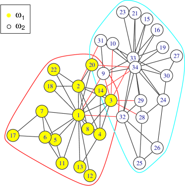
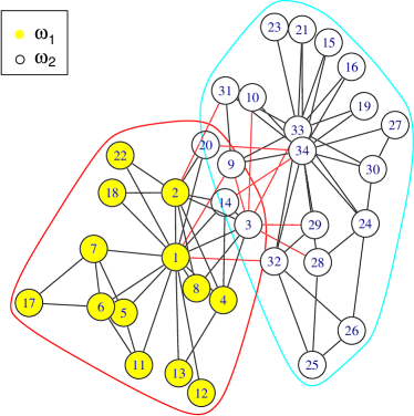
a. Original network

b. Results by FCMdd

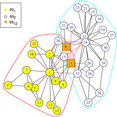
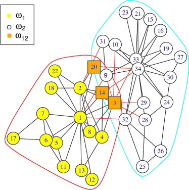
c. Results by MECM

d. Results by ECMdd

Figure 1: The Karate Club network. The parameters of MECM are $\alpha=1.5,\beta=2,\delta=100,\eta=0.9,\gamma=0.05$. In ECMdd, $\alpha=0.05,\beta=2,\delta=100,\eta=1,\gamma=1$, while in FCMdd, $\beta=2$.

IV-B Countries data

In this section we will test on a direct relational data set, referred as the benchmark data set Countries Data [1, 11]. The task is to group twelve countries into clusters based on the pairwise relationships as given in Table IV, which is in fact the average dissimilarity scores on some dimensions of quality of life provided subjectively by students in a political science class. Generally, these countries are classified into three categories: Western, Developing and Communist. We test the performances of FCMdd and ECMdd with two different sets of initial representative countries which are $\Delta_{1}$= $\{\text{C10: USSR; C8: Israel; C7: India}\}$ and $\Delta_{2}$ = $\{\text{C6: France; C4: Cuba; C1: Belgium}\}$. The three countries in $\Delta_{1}$ are well separated. On the contrary, for the countries in $\Delta_{2}$, Belgium is similar to France, which makes two initial medoids of three are very close in terms of the given dissimilarities. The parameters are set as $\beta=2$ for FCMdd, and $\beta=2,\alpha=0.95,\eta=1,\gamma=1$ for ECMdd.

TABLE IV: Countries data: dissimilarity matrix.

	Countries	C1	C2	C3	C4	C5	C6	C7	C8	C9	C10	C11	C12
1	C1: Belgium:	0.00	5.58	7.00	7.08	4.83	2.17	6.42	3.42	2.50	6.08	5.25	4.75
2	C2: Brazil	5.58	0.00	6.50	7.00	5.08	5.75	5.00	5.50	4.92	6.67	6.83	3.00
3	C3: China	7.00	6.50	0.00	3.83	8.17	6.67	5.58	6.42	6.25	4.25	4.50	6.08
4	C4: Cuba	7.08	7.00	3.83	0.00	5.83	6.92	6.00	6.42	7.33	2.67	3.75	6.67
5	C5: Egypt	4.83	5.08	8.17	5.83	0.00	4.92	4.67	5.00	4.50	6.00	5.75	5.00
6	C6: France	2.17	5.75	6.67	6.92	4.92	0.00	6.42	3.92	2.25	6.17	5.42	5.58
7	C7: India	6.42	5.00	5.58	6.00	4.67	6.42	0.00	6.17	6.33	6.17	6.08	4.83
8	C8: Israel	3.42	5.50	6.42	6.42	5.00	3.92	6.17	0.00	2.75	6.92	5.83	6.17
9	C9: USA	2.50	4.92	6.25	7.33	4.50	2.25	6.33	2.75	0.00	6.17	6.67	5.67
10	C10: USSR	6.08	6.67	4.25	2.67	6.00	6.17	6.17	6.92	6.17	0.00	3.67	6.50
11	C11: Yugoslavia	5.25	6.83	4.50	3.75	5.75	5.42	6.08	5.83	6.67	3.67	0.00	6.92
12	C12: Zaire	4.75	3.00	6.08	6.67	5.00	5.58	4.83	6.17	5.67	6.50	6.92	0.00

The results of FCMdd and ECMdd are given in Table V and Table VI respectively. It can be seen that FCMdd is very sensitive to initializations. When the initial prototypes are well set (the case of $\Delta_{1}$), the obtained partition is reasonable. However, the clustering results become worse when the initial medoids are not ideal (the case of $\Delta_{2}$). In fact two of the three medoids are not changed during the update process of FCMdd when using initial prototype set $\Delta_{2}$. This example illustrates that FCMdd is quite easy to be stuck in a local minimum. For ECMdd, the credal partitions are the same with different initializations. The pignistic probabilities are also displayed in Table VI, which could be regarded as membership values in fuzzy partitions. The country Egypt is clustered into imprecise class {1, 2}, which indicating that Egypt is not so well belongs to Developing or Western alone, but belongs to both categories. This result is consistent with the fact shown from the dissimilarity matrix: Egypt is similar to both USA and India, but has the largest dissimilarity to China. From this experiment we could conclude that ECMdd is more robust to the initializations than FCMdd.

From Table VI we can also see the medoid of each class. For instance, China is the medoid of its cluster (Communist countries) no matter which initial prototype set is used. This reflects the important role of China in communist countries and it has significant communist characters.

TABLE V: Clustering results of FCMdd for countries data. The prototype (medoid) of each class is marked with *.

		FCMdd with $\Delta_{1}$						FCMdd with $\Delta_{2}$
	Countries	$u_{i1}$	$u_{i2}$	$u_{i3}$	Label	Medoids		$u_{i1}$	$u_{i2}$	$u_{i3}$	Label	Medoids
1	C1: Belgium	0.4773	0.2543	0.2685	1	-		1.0000	0.0000	0.0000	1	*
2	C6: France	0.4453	0.2719	0.2829	1	-		0.0000	1.0000	0.0000	2	*
3	C8: Israel	1.0000	0.0000	0.0000	1	*		0.4158	0.3627	0.2215	1	-
4	C9: USA	0.5319	0.2311	0.2371	1	-		0.4078	0.4531	0.1391	2	-
5	C3: China	0.2731	0.3143	0.4126	3	-		0.2579	0.2707	0.4714	3	-
6	C4: Cuba	0.2235	0.2391	0.5374	3	-		0.0000	0.0000	1.0000	3	*
7	C10: USSR	0.0000	0.0000	1.0000	3	*		0.2346	0.2312	0.5342	3	-
8	C11: Yugoslavia	0.2819	0.2703	0.4478	3	-		0.2969	0.2875	0.4156	3	-
9	C2: Brazil	0.3419	0.3761	0.2820	2	-		0.3613	0.3506	0.2880	1	-
10	C5: Egypt	0.3444	0.3687	0.2870	2	-		0.3558	0.3493	0.2948	1	-
11	C7: India	0.0000	1.0000	0.0000	2	*		0.3257	0.3257	0.3485	3	-
12	C12: Zaire	0.3099	0.3959	0.2942	2	-		0.3901	0.3321	0.2778	1	-

TABLE VI: Clustering results of ECMdd for countries data. The prototype (medoid) of each class is marked with *. The Label {1, 2} represents the imprecise class expressing the uncertainty on class 1 and class 2.

		ECMdd with $\Delta_{1}$						ECMdd with $\Delta_{2}$
	Countries	$BetP_{i1}$	$BetP_{i2}$	$BetP_{i3}$	Label	Medoids		$BetP_{i1}$	$BetP_{i2}$	$BetP_{i3}$	Label	Medoids
1	C1: Belgium	1.0000	0.0000	0.0000	1	*		1.0000	0.0000	0.0000	1	*
2	C6: France	0.4932	0.2633	0.2435	1	-		0.5149	0.2555	0.2297	1	-
3	C8: Israel	0.4144	0.3119	0.2738	1	-		0.4231	0.3051	0.2719	1	-
4	C9: USA	0.4503	0.2994	0.2503	1	-		0.4684	0.2920	0.2396	1	-
5	C3: China	0.2323	0.2294	0.5383	3	*		0.0000	0.0000	1.0000	3	*
6	C4: Cuba	0.2778	0.2636	0.4586	3	-		0.2899	0.2794	0.4307	3	-
7	C10: USSR	0.2509	0.2260	0.5231	3	-		0.3167	0.2849	0.3984	3	-
8	C11: Yugoslavia	0.3478	0.2488	0.4034	3	-		0.3579	0.2526	0.3895	3	-
9	C2: Brazil	0.0000	1.0000	0.0000	2	*		0.0000	1.0000	0.0000	2	*
10	C5: Egypt	0.3755	0.3686	0.2558	{1, 2}	-		0.3845	0.3777	0.2378	{1, 2}	-
11	C7: India	0.3125	0.3650	0.3226	2	-		0.2787	0.3740	0.3473	2	-
12	C12: Zaire	0.3081	0.4336	0.2583	2	-		0.3068	0.4312	0.2619	2	-

IV-C UCI data sets

Finally the clustering performance of different methods will be compared on two benchmark UCI relational data sets: “Cat cortex” data set and “Protein” data set. The given information for these data sets is pair-wise relationship values. For the former it is a matrix of connection strengths between 65 cortical areas of the cat brain, while for the latter is a dissimilarity matrix measuring the structural proximity of 213 proteins sequences. The comparison results by different evaluation indices are displayed in Figure 2. For ECMdd and MECM, the classical Precision (P), Recall (R) and Rand Index (RI) are calculated based on the pignistic probabilities, and the corresponding evidential indices are obtained from the hard credal partition [4]. As it can be seen, the three classical measures are almost the same for all the methods. This reflects that pignistic probabilities play a similar role as fuzzy membership. But we can see that for ECMdd and MECM, EP is significantly high. Such effect can be attributed to the introduced imprecise clusters which enable us to make a compromise decision between hard ones. But as many points are clustered into imprecise classes, the evidential recall value is low. The performance of ECMdd is slightly better than MECM. But we know the expression of imprecise classes of ECMdd is more simple than that of MECM and from the experiment it proves that ECMdd is more efficient than MECM in terms of executing time.

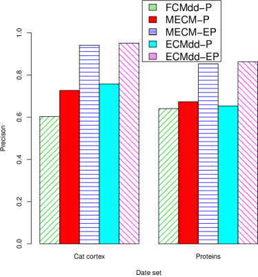
a. Precision

b. Recall

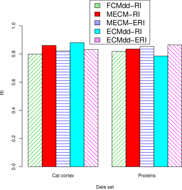
c. RI

Figure 2: The clustering results for two UCI data sets.

V Conclusion

In this paper, the evidential $c$-medoids clustering is proposed as a new medoid-based clustering algorithm. The proposed approach is the extensions of crisp $c$-medoids and fuzzy $c$-medoids on the framework of belief function theory. By the introduced imprecise clusters, we could find some overlapped and indistinguishable clusters for uncertain patterns. This results in higher accuracy of the specific decisions. The experimental results illustrates the advantages of credal partitions by ECMdd. In real applications, using only one medoid may not adequately model different types of group structure and hence limits the clustering performance on complex data sets. Therefore, we intend to include the feature of multiple prototype representation of classes in our future research work.

References

- [1] L. Kaufman and P. J. Rousseeuw, Finding groups in data: an introduction to cluster analysis. John Wiley & Sons, 2009, vol. 344.
- [2] R. Krishnapuram, A. Joshi, O. Nasraoui, and L. Yi, “Low-complexity fuzzy relational clustering algorithms for web mining,” Fuzzy Systems, IEEE Transactions on, vol. 9, no. 4, pp. 595–607, 2001.
- [3] Z.-g. Liu, Q. Pan, J. Dezert, and G. Mercier, “Credal classification rule for uncertain data based on belief functions,” Pattern Recognition, vol. 47, no. 7, pp. 2532–2541, 2014.
- [4] M.-H. Masson and T. Denoeux, “ECM: An evidential version of the fuzzy -means algorithm,” Pattern Recognition, vol. 41, no. 4, pp. 1384–1397, 2008.
- [5] Z.-g. Liu, Q. Pan, J. Dezert, and G. Mercier, “Credal -means clustering method based on belief functions,” Knowledge-Based Systems, vol. 74, pp. 119–132, 2015.
- [6] K. Zhou, A. Martin, and Q. Pan, “Evidential communities for complex networks,” in Information Processing and Management of Uncertainty in Knowledge-Based Systems. Springer, 2014, pp. 557–566.
- [7] K. Zhou, A. Martin, Q. Pan, and Z.-g. Liu, “Median evidential -means algorithm and its application to community detection,” Knowledge-Based Systems, vol. 74, pp. 69–88, 2015.
- [8] T. Denoeux, “Maximum likelihood estimation from uncertain data in the belief function framework,” Knowledge and Data Engineering, IEEE Transactions on, vol. 25, no. 1, pp. 119–130, 2013.
- [9] K. Zhou, A. Martin, and Q. Pan, “Evidential-EM algorithm applied to progressively censored observations,” in Information Processing and Management of Uncertainty in Knowledge-Based Systems. Springer, 2014, pp. 180–189.
- [10] P. Smets, “Decision making in the tbm: the necessity of the pignistic transformation,” International Journal of Approximate Reasoning, vol. 38, no. 2, pp. 133–147, 2005.
- [11] J.-P. Mei and L. Chen, “Fuzzy clustering with weighted medoids for relational data,” Pattern Recognition, vol. 43, no. 5, pp. 1964–1974, 2010.
- [12] M. Mendes and L. Sacks, “Evaluating fuzzy clustering for relevance-based information access,” in Fuzzy Systems, 2003. FUZZ’03. The 12th IEEE International Conference on, vol. 1. IEEE, 2003, pp. 648–653.
- [13] P. Jaccard, “The distribution of the flora in the alpine zone. 1,” New phytologist, vol. 11, no. 2, pp. 37–50, 1912.
- [14] T. Zhou, L. Lü, and Y.-C. Zhang, “Predicting missing links via local information,” The European Physical Journal B-Condensed Matter and Complex Systems, vol. 71, no. 4, pp. 623–630, 2009.
- [15] Y. Pan, D.-H. Li, J.-G. Liu, and J.-Z. Liang, “Detecting community structure in complex networks via node similarity,” Physica A: Statistical Mechanics and its Applications, vol. 389, no. 14, pp. 2849–2857, 2010.
- [16] Y. Hu, M. Li, P. Zhang, Y. Fan, and Z. Di, “Community detection by signaling on complex networks,” Physical Review E, vol. 78, no. 1, pp. 016 115–1–8, 2008.