Theory of Pulsed Four-Wave-Mixing in One-dimensional Silicon Photonic Crystal Slab Waveguides

Abstract

We present a comprehensive theoretical analysis and computational study of four-wave mixing (FWM) of optical pulses co-propagating in one-dimensional silicon photonic crystal waveguides (Si-PhCWGs). Our theoretical analysis describes a very general set-up of the interacting optical pulses, namely we consider nondegenerate FWM in a configuration in which at each frequency there exists a superposition of guiding modes. We incorporate in our theoretical model all relevant linear optical effects, including waveguide loss, free-carrier (FC) dispersion and FC absorption, nonlinear optical effects such as self- and cross-phase modulation (SPM, XPM), two-photon absorption (TPA), and cross-absorption modulation (XAM), as well as the coupled dynamics of FCs and optical field. In particular, our theoretical analysis based on the coupled-mode theory provides rigorously derived formulae for linear dispersion coefficients of the guiding modes, linear coupling coefficients between these modes, as well as the nonlinear waveguide coefficients describing SPM, XPM, TPA, XAM, and FWM. In addition, our theoretical analysis and numerical simulations reveal key differences between the characteristics of FWM in the slow- and fast-light regimes, which could potentially have important implications to the design of ultra-compact active photonic devices.

I Introduction

One of the most promising applications of photonics is the development of ultra-compact optical interconnects for chip-to-chip and even intra-chip communications. The driving forces behind research in this area are the perceived limitations at high frequency of currently used copper interconnects hmh01pieee , combined with a rapidly increasing demand to move huge amounts of data within increasingly more confined yet increasingly intricate communication architectures. An approach showing great potential towards developing optical interconnects at chip scale is based on high-index contrast optical waveguides, such as silicon photonic waveguides (Si-PhWGs) implemented on the silicon-on-insulator material platform lll00apl ; apc02ptl . Among key advantages provided by this platform are the increased potential for device integration facilitated by the enhanced confinement of the optical field achievable in high-index contrast photonic structures, as well as the particularly large optical nonlinearity of silicon, which makes it an ideal material for active photonic devices. Many of the basic device functionalities required in networks-on-chip have in fact already been demonstrated using Si-PhWGs, including parametric amplification cdr03oe ; edo04oe ; rjl05n ; fts06n ; lov10np , optical modulation cir95ptl ; ljl04n ; xsp05n , pulse compression cph06ptl ; m08ptl , supercontinuum generation bkr04oe ; hcl07oe , pulse self-steepening plo09ol , modulational instability pco06ol , and four-wave mixing (FWM) fys05oe ; edo05oe ; fts07oe ; zpm10np ; dog12oe ; for a review of optical properties of Si-PhWGs see opd09aop . However, since the parameter space of Si-PhWGs is rather limited, there is little room to engineer their optical properties.

A promising solution to this problem has its roots in the advent of photonic crystals (PhCs) in the late 80’s y87 ; j87 . Thus, by patterning an optical medium in a periodic manner, with the spatial periods of the pattern being comparable to the operating optical wavelength, the optical properties of the resulting medium can be modified and engineered to a remarkable extent. Following this approach, a series of photonic devices have been demonstrated using PhCs, including optical waveguides and bends mck96prl ; lch98s ; bfy99el ; mck99prb ; cn00prb , optical micro-cavities fvf97nat ; pls99s ; aas03nat ; rsl04nat ; ysh04nat , and optical filters fvj99prb ; cmi01apl . One of the most effective approaches to affect the optical properties of PhCs is to modify the group-velocity (GV), $v_{g}$, of the propagating modes. Unlike the case of waves propagating in regular optical media, whose GV can hardly be altered, by varying the geometrical parameters of PhCs one can tune the corresponding GV over many orders of magnitude. Perhaps the most noteworthy implication of the existence of optical modes with significantly reduced GV, the so-called slow-light sj04nm ; k08nphot ; b08nphot , is that both linear and nonlinear optical effects can be dramatically enhanced in the slow-light regime nys01prl ; sjf02josab ; pbo03ol ; pbo04oe ; vbh05n ; myp06ol ; cmg09nphot ; rls11prb .

One of the most important nonlinear optical process, as far as nonlinear optics applications are concerned, is FWM. In the generic case, it consists of the combination of two photons with frequencies, $\omega_{1}$ and $\omega_{2}$, belonging to two pump continuous-waves (CWs) or pulses, followed by the generation of a pair of photons with frequencies $\omega_{3}$ and $\omega_{4}$. The energy conservation requires that $\omega_{1}+\omega_{2}=\omega_{3}+\omega_{4}$. In practice, however, an easier to implement FWM configuration is usually employed, namely degenerate FWM. In this case one uses just one pump with frequency, $\omega_{p}$, the generated photons belonging to a signal ($\omega_{s}$) and an idler ($\omega_{i}$) beam; in this case the conservation of the optical energy is expressed as: $2\omega_{p}=\omega_{s}+\omega_{i}$. Among the most important applications of degenerate FWM it is noteworthy to mention optical amplification, wavelength generation and conversion, phase conjugation, generation of squeezed states, and supercontinuum generation. While FWM has been investigated theoretically and experimentally in PhC waveguides myk10oe ; ssv10oe ; meg10oe ; jli11oe ; csl12oe and long-period Bragg waveguides dog12oe ; lzd14ol , a comprehensive theory of FWM in silicon PhC waveguides (Si-PhCWGs), which rigorously incorporates in a unitary way all relevant linear and nonlinear optical effects as well as the influence of photogenerated free-carriers (FCs) on the pulse dynamics is not available yet.

In this article we introduce a rigorous theoretical model that describes FWM in Si-PhCWGs. Our model captures the influence on the FWM process of linear optical effects, including waveguide loss, FC dispersion (FCD) and FC absorption (FCA), nonlinear optical effects such as self- and cross-phase modulation (SPM, XPM), two-photon absorption (TPA), and cross-absorption modulation (XAM), as well as the mutual interaction between FCs and optical field. We also illustrate how our model can be applied to investigate the characteristics of FWM in the slow- and fast-light regimes, showing among other things that by incorporating the effects of FCs on the optical pulse dynamics new physics emerge. One noteworthy example in this context is that the well-known linear dependence of FCA on $v_{g}^{-1}$ is replaced in the slow-light regime by a $v_{g}^{-3}$ power-law dependence.

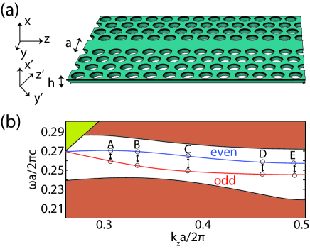
Figure 1: (a) Geometry of the 1D Si-PhC slab waveguide. The height of the slab is $h=0.6a$ and the radius of the holes is $r=0.22a$. The primed coordinate system shows the principal axes of the Si crystal with the input facet of the waveguide in the (1$\bar{1}$0) plane of the Si crystal lattice. (b) Projected band structure. Dark yellow and brown areas correspond to slab leaky and guiding modes, respectively. The red and blue curves represent the guiding modes of the 1D waveguides.

The remaining of the paper is organized as follows. In the next section we present the optical properties of the PhC waveguide considered in this work. Then, in Sec. III, we develop the theory of pulsed FWM in Si-PhCWGs whereas the particular case of degenerate FWM is analyzed in Sec. IV. Then, in Sec. V, we apply these theoretical tools to explore the physical conditions in which efficient FWM can be achieved. The results are subsequently used, in Sec. VI, to study via numerical simulations the main properties of pulsed FWM in Si-PhCWGs. We conclude our paper by summarizing in the last section the main findings of our article and discussing some of their implications to future developments in this research area. Finally, an averaged model that can be used in the case of broad optical pulses is presented in an Appendix.

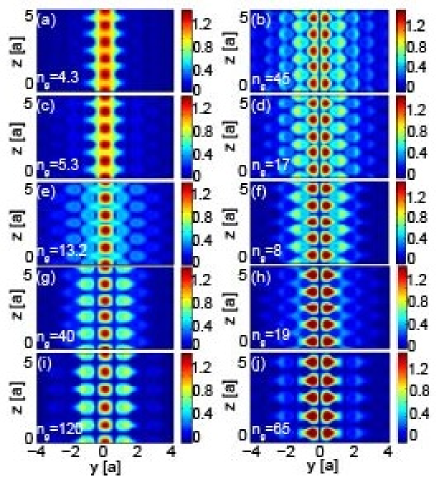
Figure 2: Left (right) panels show the amplitude of the normalized magnetic field $H_{x}$ of the $y$-odd ($y$-even) mode, calculated in the plane $x=0$ for five different values of the propagation constant, $k_{z}$. From top to bottom, the panels correspond to the Bloch modes indicated in Fig. 1(b) by the circles A, B, C, D, and E, respectively.

II Description of the photonic crystal waveguide

In this section we present the geometrical and material properties of the PhC waveguide considered in this work, as well as the physical properties of its optical modes. Thus, our Si-PhCWG consists of a one-dimensional (1D) waveguide formed by introducing a line defect in a two-dimensional (2D) honeycomb-type periodic lattice of air holes in a homogeneous slab made of silicon (a so-called W1 PhC waveguide). The line defect is oriented along the $z$-axis, which is chosen to coincide with one of the $\Gamma K$ symmetry axes of the crystal, and is created by filling in a row of holes [see Fig. 1(a)]. The slab height is $h=0.6a$ and the radius of the holes is $r=0.22a$, where $a=$412\text{\,}\mathrm{nm}$$ is the lattice constant, whereas the index of refraction of silicon is $n_{\mathrm{Si}}\equiv n=3.48$.

The defect line breaks the discrete translational symmetry of the photonic system along the $y$-axis, so that the optical modes of the waveguide are invariant only to discrete translation along the $z$-axis j08book . Moreover, based on experimental considerations, we restrict our analysis to in-plane wave propagation, namely the wave vector, $\mathbf{k}$, lies in the $x=0$ plane. The $k_{z}$ component, on the other hand, can be restricted to the first Brillouin zone, $k_{z}\in[-\pi/a,\pi/a]$, which is an immediate consequence of the Bloch theorem. Under these circumstances, we determined numerically the photonic band structure of the system and the guiding optical modes of the waveguide using MPB, a freely available code based on the plane-wave expansion (PWE) method jj01oe . To be more specific, we used a supercell with size of $6a\times 19\sqrt{3}/2a\times a$ along the $x$-, $y$-, and $z$-axis, respectively, the corresponding step size of the computational grid being $a/60$, $a\sqrt{3}/120$, and $a/60$, respectively. Figure 1(b) summarizes the results of these calculations. Thus, the waveguide has two fundamental TE-like optical guiding modes located in the band-gap of the unperturbed PhC, one $y$-even and the other one $y$-odd.

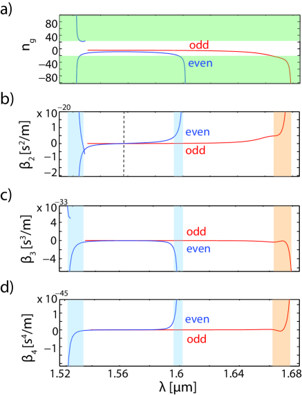
Figure 3: (a), (b), (c), and (d) Frequency dependence of waveguide dispersion coefficients $n_{g}$, $\beta_{2}$, $\beta_{3}$, and $\beta_{4}$, respectively, determined for the even and odd modes. Light green, blue, and red shaded regions correspond to slow-light regime, defined as $n_{g}>20$. The dashed vertical line in panel (b) indicates the zero-GVD wavelength.

In order to better understand the physical properties of the optical guiding modes, we plot in Fig. 2 the profile of the magnetic field $H_{x}$, which is its only nonzero component in the $x=0$ symmetry plane. These field profiles, calculated for several values of $k_{z}$, show that although the optical field is primarily confined at the location of the defect (waveguide), for some values of $k_{z}$ it is rather delocalized in the transverse direction. This field delocalization effect is particularly strong in the spectral domains where the modal dispersion curves are relatively flat, namely in the so-called slow-light regime, and increases when the group index of the mode, defined as $n_{g}=c/v_{g}$, increases.

The dispersion effects upon pulse propagation in the waveguide are characterized by the waveguide dispersion coefficients, defined as $\beta_{n}=d^{n}k_{z}/d\omega^{n}$. In particular, the first-order dispersion coefficient is related to the pulse GV via $\beta_{1}=1/v_{g}$, whereas the second-order dispersion coefficient, $\beta_{2}$, quantifies the GV dispersion (GVD) as well as pulse broadening effects. The wavelength dependence of the first four dispersion coefficients, determined for both guided modes, is presented in Fig. 3, the shaded areas indicating the spectral regions of slow-light. For the sake of clarity, we set the corresponding threshold to $c/v_{g}=20$, that is the slow-light regime is defined by $n_{g}>20$. As it can be seen in Fig. 3, the even mode possesses two slow-light regions, one located at the band-edge ($\lambda\approx$1.6\text{\,}\mathrm{\SIUnitSymbolMicro m}$$) and the other one at $k_{z}\approx 0.3(2\pi/a)$, i.e. $\lambda\approx$1.52\text{\,}\mathrm{\SIUnitSymbolMicro m}$$, whereas the odd mode contains only one such spectral domain located at the band-edge ($\lambda\approx$1.67\text{\,}\mathrm{\SIUnitSymbolMicro m}$$). Moreover, the even mode can have both positive and negative GVD, the zero-GVD point being at $\lambda=$1.56\text{\,}\mathrm{\SIUnitSymbolMicro m}$$, whereas the odd mode has normal GVD ($\beta_{2}>0$) throughout. Since usually efficient FWM can only be achieved in the anomalous GVD regime ($\beta_{2}<0$), we will assume that the interacting pulses propagate in the even mode unless otherwise is specified.

III Derivation of the Mathematical Model

This section is devoted to the derivation of a system of coupled-mode equations describing the co-propagation of a set of mutually interacting optical pulses in a Si-PhCWG, as well the influence of photogenerated FCs on the pulse evolution. We will derive these coupled-mode equations in the most general setting, namely the nondegenerate FWM, then show how they can be applied to a particular case most used in practice, the so-called degenerate FWM configuration. Our derivation follows the general approach used to develop a theoretical model for pulse propagation in silicon waveguides with uniform cross-section cpo06jqe and Si-PhCWGs pmw10jstqe .

III.1 Optical modes of photonic crystal waveguides

In the presence of an external perturbation described by the polarization, $\mathbf{P}_{\mathrm{pert}}(\mathbf{r},\omega)$, the electromagnetic field of guiding modes with frequency, $\omega$, is described by the Maxwell equations, which in the frequency domain can be written in the following form:

$$\nabla\times\mathbf{E}(\mathbf{r},\omega)=i\omega\mu\mathbf{H}(\mathbf{r},\omega),$$ (1a)

$$\nabla\times\mathbf{H}(\mathbf{r},\omega)=-i\omega[\epsilon_{c}(\mathbf{r},\omega)\mathbf{E}(\mathbf{r},\omega)+\mathbf{P}_{\mathrm{pert}}(\mathbf{r},\omega)],$$ (1b)

where $\mu$ is the magnetic permeability, which in the case of silicon and other nonmagnetic materials can be set to $\mu=\mu_{0}$, $\epsilon_{c}(\mathbf{r},\omega)$ is the dielectric constant of the PhC, and $\mathbf{E}$ and $\mathbf{H}$ are the electric and magnetic fields, respectively. In our case, $\mathbf{P}_{\mathrm{pert}}$ is the sum of polarizations describing the refraction index change induced by photogenerated FCs and nonlinear (Kerr) effects.

In order to understand how the modes of the PhC waveguide are affected by external perturbations, let us consider first the unperturbed system, that is $\mathbf{P}_{\mathrm{pert}}=0$. Thus, let us assume that, at the frequency $\omega$, the unperturbed PhC waveguide has $M$ guiding modes. It follows then from the Bloch theorem that the fields of these modes can be written as:

$$\mathbf{E}_{m\sigma}(\mathbf{r},\omega)=\mathbf{e}_{m\sigma}(\mathbf{r},\omega)e^{i\sigma\beta_{m}z},~{}~{}~{}m=1,2,\ldots,M,$$ (2a)

$$\mathbf{H}_{m\sigma}(\mathbf{r},\omega)=\mathbf{h}_{m\sigma}(\mathbf{r},\omega)e^{i\sigma\beta_{m}z},~{}~{}~{}m=1,2,\ldots,M,$$ (2b)

where $\beta_{m}$ is the $m$th mode propagation constant and $\sigma=+$ ($\sigma=-$) denotes forward (backward) propagating modes. Here, we consider that the harmonic time dependence of the fields was chosen as $e^{-i\omega t}$. The mode amplitudes $\mathbf{e}_{m\sigma}$ and $\mathbf{h}_{m\sigma}$ are periodic along the $z$-axis, with period $a$. Moreover, the forward and backward propagating modes obey the following symmetry relations:

$$\mathbf{e}_{m-}(\mathbf{r},\omega)=\mathbf{e}_{m+}^{*}(\mathbf{r},\omega),$$ (3a)

$$\mathbf{h}_{m-}(\mathbf{r},\omega)=-\mathbf{h}_{m+}^{*}(\mathbf{r},\omega),$$ (3b)

where the symbol “^∗” denotes complex conjugation. As such, one only has to determine either the forward or the backward propagating modes.

The guiding modes can be orthogonalized, the most commonly used normalization convention being

$$\frac{1}{4}\int_{S}\left(\mathbf{e}_{m\sigma}\times\mathbf{h}_{m^{\prime}\sigma^{\prime}}^{*}+\mathbf{e}_{m^{\prime}\sigma^{\prime}}^{*}\times\mathbf{h}_{m\sigma}\right)\cdot\hat{\mathbf{z}}dS=\sigma P_{m}\delta_{\sigma\sigma^{\prime}}\delta_{mm^{\prime}},$$ (4)

where $P_{m}$ is the power carried by the $m$th mode. This mode power is related to the mode energy contained in one unit cell of the PhC waveguide, $W_{m}$, via the relation:

$$P_{m}=\frac{W_{m}^{\mathrm{el}}+W_{m}^{\mathrm{mag}}}{a}v_{g}=\frac{2W_{m}^{\mathrm{el}}}{a}v_{g}=\frac{2W_{m}^{\mathrm{mag}}}{a}v_{g},$$ (5)

where

$$W_{m}^{\mathrm{el}}=\frac{1}{4}\int_{V_{\mathrm{cell}}}\frac{\partial}{\partial\omega}(\omega\epsilon_{c})|\mathbf{e}_{m\sigma}(\mathbf{r},\omega)|^{2}dV,$$ (6a)

$$W_{m}^{\mathrm{mag}}=\frac{1}{4}\int_{V_{\mathrm{cell}}}\mu_{0}|\mathbf{h}_{m\sigma}(\mathbf{r},\omega)|^{2}dV,$$ (6b)

are the electric and magnetic energy of the mode, respectively, and $V_{\mathrm{cell}}$ is the volume of the unit cell. Note that in Eq. (5) we used the fact that the mode contains equal amounts of electric and magnetic energy.

It should be stressed that the waveguide modes defined by Eqs. (2) are exact solutions of the Maxwell equations (1) with $\mathbf{P}_{\mathrm{pert}}=0$, and thus they should not be confused with the so-called local modes of the waveguide. The latter modes correspond to waveguides whose optical properties vary adiabatically with $z$, on a scale comparable to the wavelength and have been used to describe, e.g., wave propagation in tapered waveguides s70tmtt or pulse propagation in 1D long-period Bragg gratings sse02jmo .

III.2 Perturbations of the photonic crystal waveguide

Due to the photogeneration of FCs and nonlinear optical effects, the dielectric constant of Si-PhCWGs undergoes a certain local variation, $\delta\epsilon(\mathbf{r})$, upon the propagation of optical pulses in the waveguide. The corresponding perturbation polarization, $\mathbf{P}_{\mathrm{pert}}$ in Eq. (1b), can be divided in two components according to the physical effects they describe: the linear change of the dielectric constant via generation of FCs and the nonlinearly induced variation of the index of refraction.

Assuming an instantaneous response of the medium, the linear contribution to $\mathbf{P}_{\mathrm{pert}}$, $\delta\mathbf{P}_{\mathrm{lin}}(\mathbf{r},t)$, is written as:

$$\delta\mathbf{P}_{\mathrm{lin}}(\mathbf{r},t)=\left[\delta\epsilon_{\mathrm{fc}}(\mathbf{r})+\delta\epsilon_{\mathrm{loss}}(\mathbf{r})\right]\mathbf{E}(\mathbf{r},t),$$ (7)

where cpo06jqe :

$$\delta\epsilon_{\mathrm{fc}}(\mathbf{r})=\left(2\epsilon_{0}n\delta n_{\mathrm{fc}}+i\frac{\displaystyle\epsilon_{0}cn}{\displaystyle\omega}\alpha_{\mathrm{fc}}\right)\Sigma(\mathbf{r}),$$ (8a)

$$\delta\epsilon_{\mathrm{loss}}(\mathbf{r})=i\frac{\displaystyle\epsilon_{0}cn}{\displaystyle\omega}\alpha_{\mathrm{in}}\Sigma(\mathbf{r}).$$ (8b)

Here, $\alpha_{\mathrm{in}}$ is the intrinsic loss coefficient of the waveguide and $\Sigma(\mathbf{r})$ is the characteristic function of the domain where FCs can be generated, namely $\Sigma=1$ in the domain occupied by Si and $\Sigma=0$ otherwise. Based on the Drude model, the FC-induced change of the index of refraction, $\delta n_{\mathrm{fc}}$, and FC losses, $\alpha_{\mathrm{fc}}$, are given by sb87jqe :

$$\delta n_{\mathrm{fc}}=-\frac{\displaystyle e^{2}}{\displaystyle 2\epsilon_{0}n\omega^{2}}\left(\frac{N_{e}}{m_{ce}}+\frac{N_{h}^{0.8}}{m_{ch}}\right),$$ (9a)

$$\alpha_{\mathrm{fc}}=\frac{\displaystyle e^{3}}{\displaystyle\epsilon_{0}cn\omega^{2}}\left(\frac{N_{e}}{\mu_{e}m_{ce}^{2}}+\frac{N_{h}}{\mu_{h}m_{ch}^{2}}\right).$$ (9b)

Here, $e$ is the charge of the electron, $\mu_{e}$ ($\mu_{h}$) is the electron (hole) mobility, $m_{ce}=0.26m_{0}$ ($m_{ch}=0.39m_{0}$) is the conductivity effective mass of the electrons (holes), with $m_{0}$ the mass of the electron, and $N_{e}$ ($N_{h}$) is the induced variation of the electrons (holes) density (in what follows, we assume that $N_{e}=N_{h}\equiv N$).

The nonlinear contribution to $\mathbf{P}_{\mathrm{pert}}$, $\delta\mathbf{P}_{\mathrm{nl}}(\mathbf{r},t)$, is described by a third-order nonlinear susceptibility, $\hat{\chi}^{(3)}(\mathbf{r})$, and can be written as:

$$\delta\mathbf{P}_{\mathrm{nl}}(\mathbf{r},t)=\epsilon_{0}\hat{\chi}^{(3)}(\mathbf{r})\vdots\mathbf{E}(\mathbf{r},t)\mathbf{E}(\mathbf{r},t)\mathbf{E}(\mathbf{r},t).$$ (10)

The real part of the susceptibility $\hat{\chi}^{(3)}$ describes parametric optical processes such as SPM, XPM, and FWM, while the imaginary part of $\hat{\chi}^{(3)}$ corresponds to TPA and XAM. Note that in this study we neglect the stimulated Raman scattering effect as it is assumed that the frequencies of the interacting pulses do not satisfy the condition required for an efficient, resonant Raman interaction.

Since silicon belongs to the crystallographic point group $m3m$ the susceptibility tensor $\mathbb{\hat{\chi}}^{(3)}$ has 21 nonzero elements, of which only 4 are independent, namely, $\mathbb{\chi}_{1111}$, $\mathbb{\chi}_{1122}$, $\mathbb{\chi}_{1212}$, and $\mathbb{\chi}_{1221}$ b08book . In addition, the frequency dispersion of the nonlinear susceptibility can be neglected as we consider optical pulses with duration of just a few picoseconds or larger. As a consequence, the Kleinman symmetry relations imply that $\mathbb{\chi}_{1122}=\mathbb{\chi}_{1212}=\mathbb{\chi}_{1221}$. Moreover, experimental studies have shown that $\hat{\chi}^{(3)}_{1111}=2.36\hat{\chi}^{(3)}_{1122}$ zlp07apl within a broad frequency range. Therefore, the nonlinear optical effects considered here can be described by only one element of the tensor $\hat{\chi}^{(3)}$.

Because of fabrication considerations, in many instances the waveguide is not aligned with any of the crystal principal axes and as such these axes are different from the coordinate axes in which the optical modes are calculated. Therefore, one has to transform the tensor $\hat{\chi}^{(3)}$ from the crystal principal axes into the coordinate system in which the optical modes are calculated cpo06jqe ,

$$\hat{\chi}^{(3)}_{ijkl}=\hat{R}_{i\alpha}\hat{R}_{j\beta}\hat{R}_{k\gamma}\hat{R}_{l\delta}\hat{\chi}^{\prime(3)}_{\alpha\beta\gamma\delta},$$ (11)

where $\hat{\chi}^{\prime(3)}$ is the nonlinear susceptibility in the crystal principal axes and $\hat{R}$ is the rotation matrix that transforms one coordinate system into the other. In our case, $\hat{R}$ is the matrix describing a rotation with $\pi/4$ around the $x$-axis (see Fig. 1).

III.3 Coupled-mode equations for the optical field

In order to derive the system of coupled-mode equations describing pulsed FWM in Si-PhCWGs we employ the conjugated form of the Lorentz reciprocity theorem cpo06jqe ; mpw03pre ; ks07jqe ; s83book . To this end, let us consider two solutions of the Maxwell equations (1), $[\mathbf{E}_{a}(\mathbf{r},\omega_{a}),\mathbf{H}_{a}(\mathbf{r},\omega_{a})]$ and $[\mathbf{E}_{b}(\mathbf{r},\omega_{b}),\mathbf{H}_{b}(\mathbf{r},\omega_{b})]$, which correspond to two different spatial distribution of the dielectric constant, $\epsilon_{a}(\mathbf{r},\omega_{a})$ and $\epsilon_{b}(\mathbf{r},\omega_{b})$, respectively. If we insert the vector $\mathbf{F}$, defined as $\mathbf{F}=\mathbf{E}_{b}\times\mathbf{H}_{a}^{*}+\mathbf{E}_{a}^{*}\times\mathbf{H}_{b}$, in the integral identity:

$$\int_{S}\nabla\cdot\mathbf{F}dS=\frac{\displaystyle\partial}{\displaystyle\partial z}\int_{S}\mathbf{F}\cdot\hat{\mathbf{z}}dS+\oint_{\partial S}\mathbf{F}\cdot\mathbf{n}dl,$$ (12)

where $S$ is the transverse section at position, $z$, and $\partial S$ is the boundary of $S$, and use the Maxwell equations, we arrive at the following relation:

$$\frac{\displaystyle\partial}{\displaystyle\partial z} \int_{S}\mathbf{F}\cdot\hat{\mathbf{z}}dS=i\mu_{0}(\omega_{b}-\omega_{a})\int_{S}\mathbf{H}_{a}^{*}\cdot\mathbf{H}_{b}dS$$

$$+i\int_{S}(\omega_{b}\epsilon_{b}-\omega_{a}\epsilon_{a})\mathbf{E}_{a}^{*}\cdot\mathbf{E}_{b}dS-\oint_{\partial S}\mathbf{F}\cdot\mathbf{n}dl.$$ (13)

Let us consider now a nondegenerate FWM process in which two pulses at carrier frequencies $\bar{\omega}_{1}$ and $\bar{\omega}_{2}$ interact and generate two optical pulses at carrier frequencies $\bar{\omega}_{3}$ and $\bar{\omega}_{4}$, with the energy conservation expressed as $\bar{\omega}_{1}+\bar{\omega}_{2}=\bar{\omega}_{3}+\bar{\omega}_{4}$. Then, in the Lorentz reciprocity theorem given by Eq. (III.3) we choose as the first set of fields a mode of the unperturbed waveguide ($\mathbf{P}_{\mathrm{pert}}=0$), which corresponds to the frequency $\omega_{a}=\bar{\omega}_{i}$, where $\bar{\omega}_{i}$ is one of the carrier frequencies $\bar{\omega}_{1}$, $\bar{\omega}_{2}$, $\bar{\omega}_{3}$, or $\bar{\omega}_{4}$:

$$\mathbf{E}_{a}(\mathbf{r},\bar{\omega}_{i})=\frac{\mathbf{e}_{n_{i}\rho_{i}}(\mathbf{r},\bar{\omega}_{i})}{\sqrt{\bar{P}_{n_{i}}}}e^{i\rho_{i}\bar{\beta}_{n_{i}}z},$$ (14a)

$$\mathbf{H}_{a}(\mathbf{r},\bar{\omega}_{i})=\frac{\mathbf{h}_{n_{i}\rho_{i}}(\mathbf{r},\bar{\omega}_{i})}{\sqrt{\bar{P}_{n_{i}}}}e^{i\rho_{i}\bar{\beta}_{n_{i}}z},$$ (14b)

where $\rho_{i}=\pm 1$ and $n_{i}$ is an integer, $1\leq n_{i}\leq N_{i}$, $i=1,\ldots,4$, with $N_{i}$ being the number of guiding modes at the frequency $\bar{\omega}_{i}$. In Eqs. (14), and in what follows, a bar over a symbol means that the corresponding quantity is evaluated at one of the carrier frequencies.

As the second set of fields we take those that propagate in the perturbed waveguide, at the frequency $\omega_{b}=\omega$. These fields are written as a series expansion of the guiding modes at frequencies $\bar{\omega}_{i}$, $i=1,\ldots,4$, thus neglecting the frequency dispersion of the guiding modes and the radiative modes that might exist at the frequency $\omega$. This approximation is valid as long as all interacting optical pulses have narrow spectra centered at the corresponding carrier frequencies, that is the physical situation considered in this work. In particular, this modal expansion becomes less accurate when any of the pulses propagates in the slow-light regime, as generally the smaller the GV of a mode is the larger its frequency dispersion is. Thus, the second set of fields are expanded as:

$$\mathbf{E}_{b}(\mathbf{r},\omega)=\sum_{j=1}^{4}\sum_{m_{j}\sigma_{j}}a_{m_{j}\sigma_{j}}^{(j)}(z,\omega)\frac{\mathbf{e}_{m_{j}\sigma_{j}}(\mathbf{r},\bar{\omega}_{j})}{\sqrt{\bar{P}_{m_{j}}}}e^{i\sigma_{j}\bar{\beta}_{m_{j}}z},$$ (15a)

$$\mathbf{H}_{b}(\mathbf{r},\omega)=\sum_{j=1}^{4}\sum_{m_{j}\sigma_{j}}a_{m_{j}\sigma_{j}}^{(j)}(z,\omega)\frac{\mathbf{h}_{m_{j}\sigma_{j}}(\mathbf{r},\bar{\omega}_{j})}{\sqrt{\bar{P}_{m_{j}}}}e^{i\sigma_{j}\bar{\beta}_{m_{j}}z}.$$ (15b)

With the fields normalization used in Eqs. (15), the mode amplitudes $a_{m_{i}\sigma_{i}}^{(i)}(z,\omega)$, $i=1,\ldots,4$, are measured in units of $\sqrt{\mathrm{W}}$. Note that since the optical pulses are assumed to be spectrally narrow, the mode amplitudes $a_{m_{i}\sigma_{i}}^{(i)}(z,\omega)$ have negligible values except when the frequency $\omega$ lies in a narrow spectral domain centered at the carrier frequency, $\bar{\omega}_{i}$.

The dielectric constant in the two cases is $\epsilon_{a}=\bar{\epsilon}_{c}(\mathbf{r},\bar{\omega}_{i})$ and $\epsilon_{b}=\epsilon_{c}(\mathbf{r},\omega)+\delta\epsilon(\mathbf{r},\omega)$, where $\epsilon_{c}(\mathbf{r},\omega)$ is the dielectric constant of the unperturbed PhC. If the material dispersion is neglected, $\epsilon_{c}(\mathbf{r},\omega)=\epsilon_{c}(\mathbf{r},\bar{\omega}_{i})=\bar{\epsilon}_{c}(\mathbf{r})$. Inserting the fields given by Eqs. (14) and Eqs. (15) in Eq. (III.3), and neglecting the line integral in Eq. (III.3), which cancels for exponentially decaying guiding modes, one obtains the following set of coupled equations:

$$\rho_{i} \frac{\displaystyle\partial a_{n_{i}\rho_{i}}^{(i)}(z)}{\displaystyle\partial z}+\sum\limits_{\scriptsize{\begin{array}[]{c}j=1\\ j\neq i\end{array}}}^{4}\sum_{m_{j}\sigma_{j}}C_{n_{i}\rho_{i},m_{j}\sigma_{j}}^{ij}(z)$$ (18)

$$\times\left[\frac{\displaystyle\partial a_{m_{j}\sigma_{j}}^{(j)}(z)}{\displaystyle\partial z}+i(\sigma_{j}\bar{\beta}_{m_{j}}-\rho_{i}\bar{\beta}_{n_{i}})a_{m_{j}\sigma_{j}}^{(j)}(z)\right]$$

$$=B_{n_{i}\rho_{i}}^{i}a_{n_{i}\rho_{i}}^{(i)}(z)+{\sum_{jm_{j}\sigma_{j}}}^{\prime}D_{n_{i}\rho_{i},m_{j}\sigma_{j}}^{ij}a_{m_{j}\sigma_{j}}^{(j)}(z)$$

$$+\frac{i\omega e^{-i\rho_{i}\bar{\beta}_{n_{i}}z}}{4\sqrt{\bar{P}_{n_{i}}}}\int_{S}\bar{\mathbf{e}}_{n_{i}\rho_{i}}^{*}\cdot\mathbf{P}_{\mathrm{pert}}(\mathbf{r},\omega)dS,~{}~{}~{}i=1,\ldots,4,$$ (19)

where

$$C_{n_{i}\rho_{i},m_{j}\sigma_{j}}^{ij} (z)=\frac{e^{i(\sigma_{j}\bar{\beta}_{m_{j}}-\rho_{i}\bar{\beta}_{n_{i}})z}}{4\sqrt{\bar{P}_{n_{i}}\bar{P}_{m_{j}}}}$$

$$\times\int_{S}\left(\bar{\mathbf{e}}_{m_{j}\sigma_{j}}\times\bar{\mathbf{h}}_{n_{i}\rho_{i}}^{*}+\bar{\mathbf{e}}_{n_{i}\rho_{i}}^{*}\times\bar{\mathbf{h}}_{m_{j}\sigma_{j}}\right)\cdot\hat{\mathbf{z}}dS,$$ (20a)

$$B_{n_{i}\rho_{i}}^{i} =\frac{i}{4\bar{P}_{n_{i}}}\int_{S}\left[\mu_{0}(\omega-\bar{\omega}_{i})|\bar{\mathbf{h}}_{n_{i}\rho_{i}}|^{2}\right.$$

$$\left.+(\omega\epsilon_{c}-\bar{\epsilon}_{c}\bar{\omega}_{i})|\bar{\mathbf{e}}_{n_{i}\rho_{i}}|^{2}\right]dS,$$ (20b)

$$D_{n_{i}\rho_{i},m_{j}\sigma_{j}}^{ij} (z)=\frac{ie^{i(\sigma_{j}\bar{\beta}_{m_{j}}-\rho_{i}\bar{\beta}_{n_{i}})z}}{4\sqrt{\bar{P}_{n_{i}}\bar{P}_{m_{j}}}}\int_{S}\left[\mu_{0}(\omega-\bar{\omega}_{i})\right.$$

$$\left.\times\bar{\mathbf{h}}_{m_{j}\sigma_{j}}\cdot\bar{\mathbf{h}}_{n_{i}\rho_{i}}^{*}+(\omega\epsilon_{c}-\bar{\epsilon}_{c}\bar{\omega}_{i})\bar{\mathbf{e}}_{m_{j}\sigma_{j}}\cdot\bar{\mathbf{e}}_{n_{i}\rho_{i}}^{*}\right]dS.$$ (20c)

In Eq. (18) and what follows a prime symbol to a sum means that the summation is taken over all modes, except that with $j=i$, $m_{j}=n_{i}$, and $\sigma_{j}=\rho_{i}$. Moreover, in deriving the l.h.s. of Eq. (18) we used the orthogonality relation given by Eq. (4).

The time-dependent fields are obtained by integrating over all frequency components contained in the spectra of the system of interacting optical pulses:

$$\mathbf{E} (\mathbf{r},t)=\frac{1}{2}\int_{0}^{\infty}\sum_{j=1}^{4}\sum_{m_{j}\sigma_{j}}a_{m_{j}\sigma_{j}}^{(j)}(z,\omega)\frac{\mathbf{e}_{m_{j}\sigma_{j}}(\mathbf{r},\bar{\omega}_{j})}{\sqrt{\bar{P}_{m_{j}}}}$$

$$\times e^{i(\sigma_{j}\bar{\beta}_{m_{j}}z-\omega t)}d\omega+c.c.\equiv\frac{1}{2}\left[\mathbf{E}^{(+)}(\mathbf{r},t)+\mathbf{E}^{(-)}(\mathbf{r},t)\right],$$ (21a)

$$\mathbf{H} (\mathbf{r},t)=\frac{1}{2}\int_{0}^{\infty}\sum_{j=1}^{4}\sum_{m_{j}\sigma_{j}}a_{m_{j}\sigma_{j}}^{(j)}(z,\omega)\frac{\mathbf{h}_{m_{j}\sigma_{j}}(\mathbf{r},\bar{\omega}_{j})}{\sqrt{\bar{P}_{m_{j}}}}$$

$$\times e^{i(\sigma_{j}\bar{\beta}_{m_{j}}z-\omega t)}d\omega+c.c.\equiv\frac{1}{2}\left[\mathbf{H}^{(+)}(\mathbf{r},t)+\mathbf{H}^{(-)}(\mathbf{r},t)\right],$$ (21b)

where $\mathbf{E}^{(+)}(\mathbf{r},t)$, $\mathbf{H}^{(+)}(\mathbf{r},t)$ and $\mathbf{E}^{(-)}(\mathbf{r},t)$, $\mathbf{H}^{(-)}(\mathbf{r},t)$ are the positive and negative frequency parts of the spectrum, respectively.

Let us now introduce the envelopes of the interacting pulses in the time domain, $A_{n_{i}\rho_{i}}^{(i)}(z,t)$, defined as the integral of the mode amplitudes taken over the part of the spectrum that contains only positive frequencies,

$$A_{n_{i}\rho_{i}}^{(i)}(z,t)=\int_{0}^{\infty}a_{n_{i}\rho_{i}}^{(i)}(z,\omega)e^{-i(\omega-\bar{\omega}_{i})t}d\omega.$$ (22)

With this definition, the time-dependent fields given in Eqs. (21) become:

$$\mathbf{E}(\mathbf{r},t)= \frac{1}{2}\sum_{j=1}^{4}\sum_{m_{j}\sigma_{j}}A_{m_{j}\sigma_{j}}^{(j)}(z,t)$$

$$\times\frac{\bar{\mathbf{e}}_{m_{j}\sigma_{j}}(\mathbf{r},\bar{\omega}_{j})}{\sqrt{\bar{P}_{m_{j}}}}e^{i(\sigma_{j}\bar{\beta}_{m_{j}}z-\bar{\omega}_{j}t)}+c.c.,$$ (23a)

$$\mathbf{H}(\mathbf{r},t)= \frac{1}{2}\sum_{j=1}^{4}\sum_{m_{j}\sigma_{j}}A_{m_{j}\sigma_{j}}^{(j)}(z,t)$$

$$\times\frac{\bar{\mathbf{h}}_{m_{j}\sigma_{j}}(\mathbf{r},\bar{\omega}_{j})}{\sqrt{\bar{P}_{m_{j}}}}e^{i(\sigma_{j}\bar{\beta}_{m_{j}}z-\bar{\omega}_{j}t)}+c.c..$$ (23b)

Following the same approach, the time-dependent polarization, too, can be decomposed in two components, which contain positive and negative frequencies, that is, it can be written as:

$$\mathbf{P}_{\mathrm{pert}}(\mathbf{r},t) =\frac{1}{2}\int_{0}^{\infty}\mathbf{P}_{\mathrm{pert}}(\mathbf{r},\omega)e^{-i\omega t}d\omega+c.c.$$

$$\equiv\frac{1}{2}\left[\mathbf{P}_{\mathrm{pert}}^{(+)}(\mathbf{r},t)+\mathbf{P}_{\mathrm{pert}}^{(-)}(\mathbf{r},t)\right].$$ (24)

The next step of our derivation is to Fourier transform Eq. (18) in the time domain. To this end, we first expand the coefficients $B_{n_{i}\rho_{i}}^{i}$ and $D_{n_{i}\rho_{i},m_{j}\sigma_{j}}^{ij}$ in Taylor series, around the carrier frequency $\bar{\omega}_{i}$ [note that according to Eq. (20), $C_{n_{i}\rho_{i},m_{j}\sigma_{j}}^{ij}$ is frequency independent]:

$$B_{n_{i}\rho_{i}}^{i}=\sum_{q\geq 1} \frac{(\Delta\omega_{i})^{q}}{q!}\left.\frac{\partial^{q}B_{n_{i}\rho_{i}}^{i}}{\partial\omega^{q}}\right|_{\omega=\bar{\omega}_{i}}\equiv\sum_{q\geq 1}\frac{i\beta^{(q)i}_{n_{i}\rho_{i}}}{q!}(\Delta\omega_{i})^{q},$$ (25a)

$$D_{n_{i}\rho_{i},m_{j}\sigma_{j}}^{ij} =\sum_{q\geq 1}\frac{(\Delta\omega_{i})^{q}}{q!}\left.\frac{\partial^{q}D_{n_{i}\rho_{i},m_{j}\sigma_{j}}^{ij}}{\partial\omega^{q}}\right|_{\omega=\bar{\omega}_{i}}$$

$$\equiv\sum_{q\geq 1}\frac{i\beta^{(q)ij}_{n_{i}\rho_{i},m_{j}\sigma_{j}}}{q!}(\Delta\omega_{i})^{q},$$ (25b)

where $\Delta\omega_{i}=\omega-\bar{\omega}_{i}$, $i=1,\ldots,4$. Combining Eqs. (25a), (20), (5), and (6) leads to the following expression for the dispersion coefficients, $\beta^{(q)i}_{n_{i}\rho_{i}}$:

$$\beta^{(1)i}_{n_{i}\rho_{i}}(z)=\frac{\delta^{i}_{n_{i}}(z)}{v_{g,n_{i}}^{i}},$$ (26a)

$$\beta^{(n)i}_{n_{i}\rho_{i}}(z)=\delta^{i}_{n_{i}}(z)\frac{\partial^{n-1}}{\partial\omega^{n-1}}\left(\frac{1}{v_{g,n_{i}}^{i}}\right),~{}n\geq 2,$$ (26b)

where

$$\delta^{i}_{n_{i}}(z)= \frac{a}{4W_{m_{i}}}\int_{S}\left[\mu_{0}|\mathbf{h}_{n_{i}\rho_{i}}(\mathbf{r},\bar{\omega}_{i})|^{2}\right.$$

$$+\left.\frac{\partial}{\partial\omega}(\omega\epsilon_{c})|\mathbf{e}_{n_{i}\rho_{i}}(\mathbf{r},\bar{\omega}_{i})|^{2}\right]dS.$$ (27)

It can be easily seen from this equation that the average of $\delta^{i}_{n_{i}}(z)$ over one lattice cell of the PhC waveguide is equal to 1, i.e.,

$$\tilde{\delta}^{i}_{n_{i}}\equiv\frac{1}{a}\int_{z}^{z+a}\delta^{i}_{n_{i}}(z^{\prime})dz^{\prime}=1.$$ (28)

Here and in what follows the tilde symbol indicates that the corresponding physical quantity has been averaged over a lattice cell of the waveguide. With this notation, Eqs. (26) become:

$$\tilde{\beta}^{(1)i}_{n_{i}\rho_{i}}\equiv\beta^{i}_{1,n_{i}}=\frac{1}{v_{g,n_{i}}^{i}},$$ (29a)

$$\tilde{\beta}^{(n)i}_{n_{i}\rho_{i}}\equiv\beta^{i}_{n,n_{i}}=\frac{\partial^{n-1}\beta^{i}_{1,n_{i}}}{\partial\omega^{n-1}},~{}n\geq 2.$$ (29b)

These relations show that $\tilde{\beta}^{(n)i}_{n_{i}\rho_{i}}=\beta^{i}_{n,n_{i}}$ is the $n$th order dispersion coefficient of the waveguide mode characterized by the parameters $\{n_{i},\rho_{i}\}$, evaluated at $\omega=\bar{\omega}_{i}$.

We now multiply Eq. (18) by $e^{-i(\omega-\bar{\omega}_{i})t}$ and integrate over the positive-frequency domain. These simple calculations lead to the time-domain coupled-mode equations for the field envelopes, $A_{n_{i}\rho_{i}}^{(i)}(z,t)$:

$$\rho_{i}\frac{\displaystyle\partial A_{n_{i}\rho_{i}}^{(i)}}{\displaystyle\partial z}+\sum\limits_{\scriptsize{\begin{array}[]{c}j=1\\ j\neq i\end{array}}}^{4}\sum_{m_{j}\sigma_{j}}C_{n_{i}\rho_{i},m_{j}\sigma_{j}}^{ij}e^{-i(\bar{\omega}_{j}-\bar{\omega}_{i})t}\left[\frac{\displaystyle\partial A_{m_{j}\sigma_{j}}^{(j)}}{\displaystyle\partial z}\right.$$ (32)

$$\left.+i(\sigma_{j}\bar{\beta}_{m_{j}}-\rho_{i}\bar{\beta}_{n_{i}})A_{m_{j}\sigma_{j}}^{(j)}\right]=i\sum_{q\geq 1}\frac{\beta^{(q)i}_{n_{i}\rho_{i}}}{q!}\left(i\frac{\partial}{\partial t}\right)^{q}A_{n_{i}\rho_{i}}^{(i)}$$

$$+i\sum_{q\geq 1}{\sum_{jm_{j}\sigma_{j}}}^{\prime}\frac{\beta^{(q)ij}_{n_{i}\rho_{i},m_{j}\sigma_{j}}}{q!}e^{-i(\bar{\omega}_{j}-\bar{\omega}_{i})t}\left(i\frac{\partial}{\partial t}\right)^{q}A_{n_{j}\rho_{j}}^{(j)}$$

$$+\frac{i\bar{\omega}_{i}e^{-i(\rho_{i}\bar{\beta}_{n_{i}}z-\bar{\omega}_{i}t)}}{4\sqrt{\bar{P}_{n_{i}}}}\int_{S}\bar{\mathbf{e}}_{n_{i}\rho_{i}}^{*}\cdot\mathbf{P}_{\mathrm{pert}}^{(+)}(\mathbf{r},t)dS,~{}i=1,\ldots,4,$$ (33)

The temporal width of the pulses considered in this analysis is much smaller as compared to the nonlinear electronic response time of silicon and therefore the latter can be approximated to be instantaneous. In addition, we assume that the spectra of the interacting pulses are narrow and do not overlap. Under these circumstances, the optical pulses can be viewed as quasi-monochromatic waves and their nonlinear interactions can be treated in the adiabatic limit. Separating the nonlinear optical effects contributing to the nonlinear polarization, one can express in the time domain this polarization as bc91book :

$$\delta\mathbf{P}_{\mathrm{nl},\bar{\omega}_{i}}(\mathbf{r},t)=\frac{3}{4}\sum_{m_{i}\sigma_{i}}\epsilon_{0}\hat{\chi}^{(3)}(\bar{\omega}_{i},-\bar{\omega}_{i},\bar{\omega}_{i})\vdots\bar{\mathbf{e}}_{m_{i}\sigma_{i}}(\mathbf{r},\bar{\omega}_{j})\bar{\mathbf{e}}_{m_{i}\sigma_{i}}^{*}(\mathbf{r},\bar{\omega}_{j})\bar{\mathbf{e}}_{m_{i}\sigma_{i}}(\mathbf{r},\bar{\omega}_{j})|A_{m_{i}\sigma_{i}}^{(i)}{|}^{2}A_{m_{i}\sigma_{i}}^{(i)}\frac{e^{i\sigma_{i}\bar{\beta}_{m_{i}}z}}{\bar{P}_{m_{i}}\sqrt{\bar{P}_{m_{i}}}}$$

$$~{}+\frac{3}{2}\sum_{m_{i}\sigma_{i}}\sum\limits_{\scriptsize{\begin{array}[]{c}(p_{i}\varrho_{i})\neq(m_{i}\sigma_{i})\\ p_{i}>m_{i}\end{array}}}\epsilon_{0}\hat{\chi}^{(3)}(\bar{\omega}_{i},-\bar{\omega}_{i},\bar{\omega}_{i})\vdots\bar{\mathbf{e}}_{p_{i}\varrho_{i}}(\mathbf{r},\bar{\omega}_{i})\bar{\mathbf{e}}_{p_{i}\varrho_{i}}^{*}(\mathbf{r},\bar{\omega}_{i})\bar{\mathbf{e}}_{m_{i}\sigma_{i}}(\mathbf{r},\bar{\omega}_{i})|A_{p_{i}\varrho_{i}}^{(i)}{|}^{2}A_{m_{i}\sigma_{i}}^{(i)}\frac{e^{i\sigma_{i}\bar{\beta}_{m_{i}}z}}{\bar{P}_{p_{i}}\sqrt{\bar{P}_{m_{i}}}}$$ (36)

$$~{}+\frac{3}{2}\sum\limits_{\scriptsize{\begin{array}[]{c}j=1\\ j\neq i\end{array}}}^{4}\sum\limits_{\scriptsize{\begin{array}[]{c}m_{i}\sigma_{i}\\ p_{j}\varrho_{j}\end{array}}}\epsilon_{0}\hat{\chi}^{(3)}(\bar{\omega}_{j},-\bar{\omega}_{j},\bar{\omega}_{i})\vdots\bar{\mathbf{e}}_{p_{j}\varrho_{j}}(\mathbf{r},\bar{\omega}_{j})\bar{\mathbf{e}}_{p_{j}\varrho_{j}}^{*}(\mathbf{r},\bar{\omega}_{j})\bar{\mathbf{e}}_{m_{i}\sigma_{i}}(\mathbf{r},\bar{\omega}_{i})|A_{p_{j}\varrho_{j}}^{(j)}{|}^{2}A_{m_{i}\sigma_{i}}^{(i)}\frac{e^{i\sigma_{i}\bar{\beta}_{m_{i}}z}}{\bar{P}_{p_{j}}\sqrt{\bar{P}_{m_{i}}}}$$ (41)

$$~{}+\frac{3}{2}\sum\limits_{\scriptsize{\begin{array}[]{c}p_{j}q_{k}m_{l}\\ \varrho_{j}\tau_{k}\sigma_{l}\end{array}}}\epsilon_{0}\hat{\chi}^{(3)}(\bar{\omega}_{j},-\bar{\omega}_{k},\bar{\omega}_{l})\vdots\bar{\mathbf{e}}_{p_{j}\varrho_{j}}(\mathbf{r},\bar{\omega}_{j})\bar{\mathbf{e}}_{q_{k}\tau_{k}}^{*}(\mathbf{r},\bar{\omega}_{k})\bar{\mathbf{e}}_{m_{l}\sigma_{l}}(\mathbf{r},\bar{\omega}_{l})A_{p_{j}\varrho_{j}}^{(j)}A_{q_{k}\tau_{k}}^{(k)*}A_{m_{l}\sigma_{l}}^{(l)}$$ (44)

$$~{}~{}~{}~{}\left.\times\frac{e^{i\left[(\varrho_{j}\bar{\beta}_{p_{j}}-\tau_{k}\bar{\beta}_{q_{k}}+\sigma_{l}\bar{\beta}_{m_{l}})z-(\bar{\omega}_{j}-\bar{\omega}_{k}+\bar{\omega}_{l})t\right]}}{\sqrt{\bar{P}_{p_{j}}\bar{P}_{q_{k}}\bar{P}_{m_{l}}}}\right|_{\scriptsize{\begin{array}[]{lc}j\neq k\neq l\neq i\\ \bar{\omega}_{j}-\bar{\omega}_{k}+\bar{\omega}_{l}=\bar{\omega}_{i}\end{array}}}.$$ (47)

This expression for the nonlinear polarization accounts for the fact that the nonlinear susceptibility is invariant to frequency permutations. The first term in Eq. (III.3) represents SPM effects of the pulse envelopes, the second and third terms describe the XPM between modes with the same frequency and XPM between pulses propagating at different frequencies, respectively, whereas the last term describes FWM processes.

If one inserts in Eq. (32) the linear and nonlinear polarizations given by Eq. (7) and Eq. (III.3), respectively, then discards the fast time-varying terms, one obtains the following system of coupled equations that governs the dynamics of the mode envelopes:

$$\rho_{i}\frac{\displaystyle\partial A_{n_{i}\rho_{i}}^{(i)}}{\displaystyle\partial z}=i\sum_{q\geq 1}\frac{\beta^{(q)i}_{n_{i}\rho_{i}}}{q!}\left(i\frac{\partial}{\partial t}\right)^{q}A_{n_{i}\rho_{i}}^{(i)}$$

$$+i\sum_{q\geq 1}\sum\limits_{\scriptsize{(m_{i}\sigma_{i})\neq(n_{i}\rho_{i})}}\frac{\beta^{(q)ii}_{n_{i}\rho_{i},m_{i}\sigma_{i}}}{q!}\left(i\frac{\partial}{\partial t}\right)^{q}A_{m_{i}\sigma_{i}}^{(i)}$$

$$+i\frac{\vartheta_{n_{i}\rho_{i}}^{i}(z)}{v_{g,n_{i}}^{i}}A_{n_{i}\rho_{i}}^{(i)}+i\sum\limits_{\scriptsize{(m_{i}\sigma_{i})\neq(n_{i}\rho_{i})}}\frac{\vartheta_{n_{i}\rho_{i},m_{i}\sigma_{i}}^{i}(z)}{\sqrt{v_{g,n_{i}}^{i}v_{g,m_{i}}^{i}}}A_{m_{i}\sigma_{i}}^{(i)}$$

$$+\frac{3i\bar{\omega}_{i}}{16\epsilon_{0}a^{2}}\Bigg{\{}\sum_{m_{i}\sigma_{i}}\Bigg{[}\frac{\Gamma_{n_{i}\rho_{i},m_{i}\sigma_{i}}^{i}(z)}{v_{g,m_{i}}^{i}\sqrt{v_{g,m_{i}}^{i}v_{g,n_{i}}^{i}}}|A_{m_{i}\sigma_{i}}^{(i)}{|}^{2}A_{m_{i}\sigma_{i}}^{(i)}$$

$$+\sum\limits_{\scriptsize{\begin{array}[]{c}(p_{i}\varrho_{i})\neq(m_{i}\sigma_{i})\\ p_{i}>m_{i}\end{array}}}\frac{2\Gamma_{n_{i}\rho_{i},m_{i}\sigma_{i}p_{i}\varrho_{i}}^{i}(z)}{v_{g,p_{i}}^{i}\sqrt{v_{g,m_{i}}^{i}v_{g,n_{i}}^{i}}}|A_{p_{i}\varrho_{i}}^{(i)}{|}^{2}A_{m_{i}\sigma_{i}}^{(i)}$$ (50)

$$+\sum\limits_{\scriptsize{\begin{array}[]{c}j=1\\ j\neq i\end{array}}}^{4}\sum\limits_{\scriptsize{p_{j}\varrho_{j}}}\frac{2\Gamma_{n_{i}\rho_{i},m_{i}\sigma_{i}p_{j}\varrho_{j}}^{ij}(z)}{v_{g,p_{j}}^{j}\sqrt{v_{g,m_{i}}^{i}v_{g,n_{i}}^{i}}}|A_{p_{j}\varrho_{j}}^{(j)}{|}^{2}A_{m_{i}\sigma_{i}}^{(i)}\Bigg{]}$$ (53)

$$+\sum\limits_{\scriptsize{\begin{array}[]{c}p_{j}q_{k}m_{l}\\ \varrho_{j}\tau_{k}\sigma_{l}\end{array}}}e^{i\Delta\bar{\beta}_{n_{i}p_{j}q_{k}m_{l}}z}\frac{2\Gamma_{n_{i}\rho_{i},p_{j}\varrho_{j}q_{k}\tau_{k}m_{l}\sigma_{l}}^{jkl}(z)}{\sqrt{v_{g,p_{j}}^{j}v_{g,q_{k}}^{k}v_{g,m_{l}}^{l}v_{g,n_{i}}^{i}}}$$ (56)

$$~{}~{}~{}~{}~{}\left.\times A_{p_{j}\varrho_{j}}^{(j)}A_{q_{k}\tau_{k}}^{(k)*}A_{m_{l}\sigma_{l}}^{(l)}\right|_{j\neq k\neq l\neq i}\Bigg{\}},~{}i=1,\ldots,4,$$ (57)

where $\Delta\bar{\beta}_{n_{i}p_{j}q_{k}m_{l}}=\varrho_{j}\bar{\beta}_{p_{j}}-\tau_{k}\bar{\beta}_{q_{k}}+\sigma_{l}\bar{\beta}_{m_{l}}-\rho_{i}\bar{\beta}_{n_{i}}$ is the wavevector mismatch.

The coefficients $\vartheta_{n_{i}\rho_{i}}^{i}$ and $\vartheta_{n_{i}\rho_{i},m_{i}\sigma_{i}}^{i}$ represent the wavevector shift of the optical mode $(n_{i},\rho_{i})$ and the linear coupling constant between modes $(n_{i},\rho_{i})$ and $(m_{i},\sigma_{i})$, induced by the linear perturbations, respectively, $\Gamma_{n_{i}\rho_{i},m_{i}\sigma_{i}}^{i}$ and $\Gamma_{n_{i}\rho_{i},m_{i}\sigma_{i}p_{i}\varrho_{i}}^{i}$ describe SPM and XPM-induced coupling between modes with the same frequency, $\bar{\omega}_{i}$, respectively, $\Gamma_{n_{i}\rho_{i},m_{i}\sigma_{i}p_{j}\varrho_{j}}^{ij}$ represents the XPM-induced coupling between modes with frequencies $\bar{\omega}_{i}$ and $\bar{\omega}_{j}$, and $\Gamma_{n_{i}\rho_{i},p_{j}\varrho_{j}q_{k}\tau_{k}m_{l}\sigma_{l}}^{jkl}$ is related to the FWM interaction among the pulses. All these nonlinear coefficients have the meaning of $z$-dependent effective cubic susceptibilities. The linear and nonlinear coefficients in Eqs. (III.3) are given by the following relations:

$$\vartheta_{n_{i}\rho_{i}}^{i}(z)=\frac{\bar{\omega}_{i}a}{4\bar{W}_{n_{i}}^{i}}\int_{S}[\delta\epsilon_{\mathrm{fc}}(\mathbf{r})+\delta\epsilon_{\mathrm{loss}}(\mathbf{r})]|\mathbf{e}_{n_{i}\rho_{i}}(\bar{\omega}_{i})|^{2}dS,$$ (58a)

$$\vartheta_{n_{i}\rho_{i},m_{i}\sigma_{i}}^{i}(z)=\frac{\bar{\omega}_{i}e^{i(\sigma_{i}\bar{\beta}_{m_{i}}-\rho_{i}\bar{\beta}_{n_{i}})z}}{4\sqrt{\bar{W}_{n_{i}}^{i}\bar{W}_{m_{i}}^{i}}}$$

$$~{}~{}\times\int_{S}[\delta\epsilon_{\mathrm{fc}}(\mathbf{r})+\delta\epsilon_{\mathrm{loss}}(\mathbf{r})]\mathbf{e}_{n_{i}\rho_{i}}^{*}(\bar{\omega}_{i})\cdot\mathbf{e}_{m_{i}\sigma_{i}}(\bar{\omega}_{i})dS,$$ (58b)

$$\Gamma_{n_{i}\rho_{i},m_{i}\sigma_{i}}^{i}(z)=\frac{\epsilon_{0}^{2}a^{4}e^{i(\sigma_{i}\bar{\beta}_{m_{i}}-\rho_{i}\bar{\beta}_{n_{i}})z}}{\bar{W}_{m_{i}}^{i}\sqrt{\bar{W}_{m_{i}}^{i}\bar{W}_{n_{i}}^{i}}}\int_{S}\mathbf{e}_{n_{i}\rho_{i}}^{*}(\bar{\omega}_{i})$$

$$~{}~{}\cdot\hat{\chi}^{(3)}(\bar{\omega}_{i},-\bar{\omega}_{i},\bar{\omega}_{i})\vdots\mathbf{e}_{m_{i}\sigma_{i}}(\bar{\omega}_{i})\mathbf{e}_{m_{i}\sigma_{i}}^{*}(\bar{\omega}_{i})\mathbf{e}_{m_{i}\sigma_{i}}(\bar{\omega}_{i})dS,$$ (58c)

$$\Gamma_{n_{i}\rho_{i},m_{i}\sigma_{i}p_{i}\varrho_{i}}^{i}(z)=\frac{\epsilon_{0}^{2}a^{4}e^{i(\sigma_{i}\bar{\beta}_{m_{i}}-\rho_{i}\bar{\beta}_{n_{i}})z}}{\bar{W}_{p_{i}}^{i}\sqrt{\bar{W}_{m_{i}}^{i}\bar{W}_{n_{i}}^{i}}}\int_{S}\mathbf{e}_{n_{i}\rho_{i}}^{*}(\bar{\omega}_{i})$$

$$~{}~{}\cdot\hat{\chi}^{(3)}(\bar{\omega}_{i},-\bar{\omega}_{i},\bar{\omega}_{i})\vdots\mathbf{e}_{p_{i}\varrho_{i}}(\bar{\omega}_{i})\mathbf{e}_{p_{i}\varrho_{i}}^{*}(\bar{\omega}_{i})\mathbf{e}_{m_{i}\sigma_{i}}(\bar{\omega}_{i})dS,$$ (58d)

$$\Gamma_{n_{i}\rho_{i},m_{i}\sigma_{i}p_{j}\varrho_{j}}^{ij}(z)=\frac{\epsilon_{0}^{2}a^{4}e^{i(\sigma_{i}\bar{\beta}_{m_{i}}-\rho_{i}\bar{\beta}_{n_{i}})z}}{\bar{W}_{p_{j}}^{j}\sqrt{\bar{W}_{m_{i}}^{i}\bar{W}_{n_{i}}^{i}}}\int_{S}\mathbf{e}_{n_{i}\rho_{i}}^{*}(\bar{\omega}_{i})$$

$$~{}~{}\cdot\hat{\chi}^{(3)}(\bar{\omega}_{j},-\bar{\omega}_{j},\bar{\omega}_{i})\vdots\mathbf{e}_{p_{j}\varrho_{j}}(\bar{\omega}_{j})\mathbf{e}_{p_{j}\varrho_{j}}^{*}(\bar{\omega}_{j})\mathbf{e}_{m_{i}\sigma_{i}}(\bar{\omega}_{i})dS,$$ (58e)

$$\Gamma_{n_{i}\rho_{i},p_{j}\varrho_{j}q_{k}\tau_{k}m_{l}\sigma_{l}}^{jkl}(z)=\frac{\epsilon_{0}^{2}a^{4}}{\sqrt{\bar{W}_{p_{j}}^{j}\bar{W}_{q_{k}}^{k}\bar{W}_{m_{l}}^{l}\bar{W}_{n_{i}}^{i}}}\int_{S}\mathbf{e}_{n_{i}\rho_{i}}^{*}(\bar{\omega}_{i})$$

$$~{}~{}\cdot\hat{\chi}^{(3)}(\bar{\omega}_{j},-\bar{\omega}_{k},\bar{\omega}_{l})\vdots\mathbf{e}_{p_{j}\varrho_{j}}(\bar{\omega}_{j})\mathbf{e}_{q_{k}\tau_{k}}^{*}(\bar{\omega}_{k})\mathbf{e}_{m_{l}\sigma_{l}}(\bar{\omega}_{l})dS.$$ (58f)

While Eqs. (III.3) seem complicated, in cases of practical interest they can be considerably simplified. To be more specific, these equations describe a multitude of optical effects pertaining to both linear and nonlinear gratings, including linear coupling between modes with the same frequency, nonlinear coupling between modes with the same frequency, due to SPM and XPM effects, XPM-induced coupling between modes with different frequency, and FWM interactions. In most experimental set-ups, however, not all these linear and nonlinear effects occur simultaneously as in a generic case not all of them lead to efficient pulse interactions.

These ideas becomes clear if one inspects the exponential factors in Eqs. (58)-(58). Thus, they vary over a characteristic length comparable to the lattice constant of the PhC, namely much more rapidly as compared to the spatial variation rate of the pulse envelopes. As a result, except for the mode $(n_{i},\rho_{i})$, these linear and nonlinear coefficients cancel. There are, however, particular cases when some of these interactions are phase-matched and consequently are resonantly enhanced. To be more specific, the integrals in Eqs. (58)-(58) are periodic functions of $z$, with period $a$, so that it is possible that a Fourier component of these integrals phase-matches a specific linear or nonlinear interaction between modes (e.g., the linear coupling between two modes with the same frequency and SPM- or XPM-induced nonlinear coupling between modes). In this study, we do not consider such accidental phase-matching of mode interactions. With this in mind, we discard all terms in Eqs. (III.3) that average to zero to obtain the final form of the coupled-mode equations for the pulse envelopes:

$$i \bigg{[}\rho_{i}\frac{\displaystyle\partial A_{n_{i}\rho_{i}}^{(i)}}{\displaystyle\partial z}+\frac{\delta^{i}_{n_{i}}(z)}{v_{g,n_{i}}^{i}}\frac{\partial A_{n_{i}\rho_{i}}^{(i)}}{\partial t}\bigg{]}-\frac{\delta^{i}_{n_{i}}(z)\bar{\beta}_{2,n_{i}}}{2}\frac{\partial^{2}A_{n_{i}\rho_{i}}^{(i)}}{\partial t^{2}}$$

$$+\frac{\bar{\omega}_{i}\delta n_{\mathrm{fc}}\bar{\kappa}_{n_{i}}^{i}(z)}{nv_{g,n_{i}}^{i}}A_{n_{i}\rho_{i}}^{(i)}+\frac{ic\bar{\kappa}_{n_{i}}^{i}(z)}{2nv_{g,n_{i}}^{i}}(\alpha_{\mathrm{fc}}+\alpha_{\mathrm{in}})A_{n_{i}\rho_{i}}^{(i)}$$

$$+\gamma_{n_{i}\rho_{i}}^{i}(z)|A_{n_{i}\rho_{i}}^{(i)}{|}^{2}A_{n_{i}\rho_{i}}^{(i)}+\sum\limits_{\scriptsize{\begin{array}[]{c}(p_{i}\varrho_{i})\neq(n_{i}\rho_{i})\\ p_{i}>n_{i}\end{array}}}2\gamma_{n_{i}\rho_{i},p_{i}\varrho_{i}}^{i}(z)$$ (61)

$$\times|A_{p_{i}\varrho_{i}}^{(i)}{|}^{2}A_{n_{i}\rho_{i}}^{(i)}+\sum\limits_{\scriptsize{\begin{array}[]{c}j=1\\ j\neq i\end{array}}}^{4}\sum\limits_{\scriptsize{p_{j}\varrho_{j}}}2\gamma_{n_{i}\rho_{i},p_{j}\varrho_{j}}^{ij}(z)|A_{p_{j}\varrho_{j}}^{(j)}{|}^{2}A_{n_{i}\rho_{i}}^{(i)}$$ (64)

$$+\sum\limits_{\scriptsize{\begin{array}[]{c}p_{j}q_{k}m_{l}\\ \varrho_{j}\tau_{k}\sigma_{l}\end{array}}}2e^{i\Delta\bar{\beta}_{n_{i}p_{j}q_{k}m_{l}}z}\gamma_{n_{i}\rho_{i},p_{j}\varrho_{j}q_{k}\tau_{k}m_{l}\sigma_{l}}^{jkl}(z)$$ (67)

$$~{}~{}~{}~{}~{}\left.\times A_{p_{j}\varrho_{j}}^{(j)}A_{q_{k}\tau_{k}}^{(k)*}A_{m_{l}\sigma_{l}}^{(l)}\right|_{j\neq k\neq l\neq i}=0,~{}i=1,\ldots,4,$$ (68)

where the new parameters introduced in this equation are defined as:

$$\bar{\kappa}_{n_{i}}^{i}(z)=\frac{\epsilon_{0}an^{2}}{2\bar{W}_{n_{i}}^{i}}\int_{S_{\mathrm{nl}}}|\mathbf{e}_{n_{i}\rho_{i}}(\bar{\omega}_{i})|^{2}dS,$$ (69a)

$$\gamma_{n_{i}\rho_{i}}^{i}(z)=\frac{3\bar{\omega}_{i}\epsilon_{0}a^{2}}{16v_{g,n_{i}}^{i^{\scriptstyle 2}}}\frac{1}{\bar{W}_{n_{i}}^{i^{\scriptstyle 2}}}\int_{S_{\mathrm{nl}}}\mathbf{e}_{n_{i}\rho_{i}}^{*}(\bar{\omega}_{i})$$

$$~{}~{}\cdot\hat{\chi}^{(3)}(\bar{\omega}_{i},-\bar{\omega}_{i},\bar{\omega}_{i})\vdots\mathbf{e}_{n_{i}\rho_{i}}(\bar{\omega}_{i})\mathbf{e}_{n_{i}\rho_{i}}^{*}(\bar{\omega}_{i})\mathbf{e}_{n_{i}\rho_{i}}(\bar{\omega}_{i})dS,$$ (69b)

$$\gamma_{n_{i}\rho_{i},p_{i}\varrho_{i}}^{i}(z)=\frac{3\bar{\omega}_{i}\epsilon_{0}a^{2}}{16v_{g,n_{i}}^{i}v_{g,p_{i}}^{i}}\frac{1}{\bar{W}_{n_{i}}^{i}\bar{W}_{p_{i}}^{i}}\int_{S_{\mathrm{nl}}}\mathbf{e}_{n_{i}\rho_{i}}^{*}(\bar{\omega}_{i})$$

$$~{}~{}\cdot\hat{\chi}^{(3)}(\bar{\omega}_{i},-\bar{\omega}_{i},\bar{\omega}_{i})\vdots\mathbf{e}_{p_{i}\varrho_{i}}(\bar{\omega}_{i})\mathbf{e}_{p_{i}\varrho_{i}}^{*}(\bar{\omega}_{i})\mathbf{e}_{n_{i}\rho_{i}}(\bar{\omega}_{i})dS,$$ (69c)

$$\gamma_{n_{i}\rho_{i},p_{j}\varrho_{j}}^{ij}(z)=\frac{3\bar{\omega}_{i}\epsilon_{0}a^{2}}{16v_{g,n_{i}}^{i}v_{g,p_{j}}^{j}}\frac{1}{\bar{W}_{n_{i}}^{i}\bar{W}_{p_{j}}^{j}}\int_{S_{\mathrm{nl}}}\mathbf{e}_{n_{i}\rho_{i}}^{*}(\bar{\omega}_{i})$$

$$~{}~{}\cdot\hat{\chi}^{(3)}(\bar{\omega}_{j},-\bar{\omega}_{j},\bar{\omega}_{i})\vdots\mathbf{e}_{p_{j}\varrho_{j}}(\bar{\omega}_{j})\mathbf{e}_{p_{j}\varrho_{j}}^{*}(\bar{\omega}_{j})\mathbf{e}_{n_{i}\rho_{i}}(\bar{\omega}_{i})dS,$$ (69d)

$$\gamma_{n_{i}\rho_{i},p_{j}\varrho_{j}q_{k}\tau_{k}m_{l}\sigma_{l}}^{jkl}(z)=\frac{3\bar{\omega}_{i}\epsilon_{0}a^{2}}{16{(v_{g,p_{j}}^{j}v_{g,q_{k}}^{k}v_{g,m_{l}}^{l}v_{g,n_{i}}^{i})}^{\frac{1}{2}}}$$

$$~{}~{}\frac{1}{{(\bar{W}_{p_{j}}^{j}\bar{W}_{q_{k}}^{k}\bar{W}_{m_{l}}^{l}\bar{W}_{n_{i}}^{i})}^{\frac{1}{2}}}\int_{S_{\mathrm{nl}}}\mathbf{e}_{n_{i}\rho_{i}}^{*}(\bar{\omega}_{i})\cdot\hat{\chi}^{(3)}(\bar{\omega}_{j},-\bar{\omega}_{k},\bar{\omega}_{l})$$

$$~{}~{}\vdots\mathbf{e}_{p_{j}\varrho_{j}}(\bar{\omega}_{j})\mathbf{e}_{q_{k}\tau_{k}}^{*}(\bar{\omega}_{k})\mathbf{e}_{m_{l}\sigma_{l}}(\bar{\omega}_{l})dS.$$ (69e)

In these equations, $S_{\mathrm{nl}}(z)$ is the transverse surface of the region filled with nonlinear material. Note that the exponential factor in the term describing the FWM does not average to zero because the FWM interaction is assumed to be nearly phase-matched and therefore the exponential factor varies over a characteristic length that is much larger than the lattice constant, $a$. Importantly, the linear and nonlinear effects in Eq. (III.3) appear as being inverse proportional to the $v_{g}$ and $v_{g}^{2}$, respectively. In other words, one does not need to rely on any phenomenological considerations to describe slow-light effects, as they are naturally captured by our model.

III.4 Carriers dynamics

The last step in our derivation of the theoretical model describing FWM in Si-PhCWGs is to determine the influence of photogenerated FCs on pulse dynamics. To this end, we first find the rate at which electron-hole pairs are generated optically, via degenerate and nondegenerate TPA, and as a result of FWM. More specifically, we first multiply Eqs. (III.3), after all linear terms have been discarded, by $A_{n_{i}\rho_{i}}^{(i)*}$, then multiply the complex conjugate of Eqs. (III.3) by $A_{n_{i}\rho_{i}}^{(i)}$, and sum the results over all carrier frequencies and modes. The outcome of these simple manipulations can be cast as:

$$\frac{\displaystyle\partial}{\displaystyle\partial z}\sum_{i=1}^{4}\sum_{n_{i}\rho_{i}}\rho_{i}|A_{n_{i}\rho_{i}}^{(i)}|^{2}=-\frac{3}{8\epsilon_{0}a^{2}}\sum_{i=1}^{4}\sum_{n_{i}\rho_{i}}\bar{\omega}_{i}$$

$$\times\mathfrak{Im}\Bigg{\{}\sum_{m_{i}\sigma_{i}}\Bigg{[}\frac{\Gamma_{n_{i}\rho_{i},m_{i}\sigma_{i}}^{i}(z)}{v_{g,m_{i}}^{i}\sqrt{v_{g,m_{i}}^{i}v_{g,n_{i}}^{i}}}|A_{m_{i}\sigma_{i}}^{(i)}{|}^{2}A_{m_{i}\sigma_{i}}^{(i)}A_{n_{i}\rho_{i}}^{(i)*}$$

$$+\sum\limits_{\scriptsize{\begin{array}[]{c}(p_{i}\varrho_{i})\neq(m_{i}\sigma_{i})\\ p_{i}>m_{i}\end{array}}}\frac{2\Gamma_{n_{i}\rho_{i},m_{i}\sigma_{i}p_{i}\varrho_{i}}^{i}(z)}{v_{g,p_{i}}^{i}\sqrt{v_{g,m_{i}}^{i}v_{g,n_{i}}^{i}}}|A_{p_{i}\varrho_{i}}^{(i)}{|}^{2}A_{m_{i}\sigma_{i}}^{(i)}A_{n_{i}\rho_{i}}^{(i)*}$$ (72)

$$+\sum\limits_{\scriptsize{\begin{array}[]{c}j=1\\ j\neq i\end{array}}}^{4}\sum\limits_{\scriptsize{p_{j}\varrho_{j}}}\frac{2\Gamma_{n_{i}\rho_{i},m_{i}\sigma_{i}p_{j}\varrho_{j}}^{ij}(z)}{v_{g,p_{j}}^{j}\sqrt{v_{g,m_{i}}^{i}v_{g,n_{i}}^{i}}}|A_{p_{j}\varrho_{j}}^{(j)}{|}^{2}A_{m_{i}\sigma_{i}}^{(i)}A_{n_{i}\rho_{i}}^{(i)*}\Bigg{]}$$ (75)

$$+\sum\limits_{\scriptsize{\begin{array}[]{c}p_{j}q_{k}m_{l}\\ \varrho_{j}\tau_{k}\sigma_{l}\end{array}}}e^{i\Delta\bar{\beta}_{n_{i}p_{j}q_{k}m_{l}}z}\frac{2\Gamma_{n_{i}\rho_{i},p_{j}\varrho_{j}q_{k}\tau_{k}m_{l}\sigma_{l}}^{jkl}(z)}{\sqrt{v_{g,p_{j}}^{j}v_{g,q_{k}}^{k}v_{g,m_{l}}^{l}v_{g,n_{i}}^{i}}}$$ (78)

$$~{}~{}~{}~{}~{}\left.\times A_{p_{j}\varrho_{j}}^{(j)}A_{q_{k}\tau_{k}}^{(k)*}A_{m_{l}\sigma_{l}}^{(l)}A_{n_{i}\rho_{i}}^{(i)*}\right|_{j\neq k\neq l\neq i}\Bigg{\}}.$$ (79)

The sum in the l.h.s. of this equation represents the rate at which optical power is transferred to FCs. This power is absorbed by carriers generated in the silicon slab, in the infinitesimal volume $dV(z)=A_{\mathrm{nl}}(z)dz$, where $A_{\mathrm{nl}}(z)$ is an effective area. This area is defined in terms of the Poynting vector of the field propagating inside the silicon slab,

$$A_{\mathrm{nl}}(z)=\frac{\big{[}\int_{S_{\mathrm{nl}}}|\langle\mathbf{E}(\mathbf{r},t)\times\mathbf{H}(\mathbf{r},t)\rangle_{t}|dS\big{]}^{2}}{\int_{S_{\mathrm{nl}}}|\langle\mathbf{E}(\mathbf{r},t)\times\mathbf{H}(\mathbf{r},t)\rangle_{t}|^{2}dS}.$$ (80)

In this equation, $\langle f\rangle_{t}$ means the time average of $f$. Using Eq. (23), and taking into account the fact that $A_{n_{i}\rho_{i}}^{(i)}$ varies in time much slower than $e^{-i\bar{\omega}_{i}t}$, one can express Eq. (80) in the following form:

$$A_{\mathrm{nl}}(z)=\frac{\displaystyle\bigg{[}\int_{S_{\mathrm{nl}}}\bigg{\lvert}\sum_{i=1}^{4}\sum_{n_{i}\rho_{i}}\frac{|A_{n_{i}\rho_{i}}^{(i)}|^{2}}{\bar{P}_{n_{i}}}\mathfrak{Re}(\mathbf{e}_{n_{i}\rho_{i}}\times\mathbf{h}_{n_{i}\rho_{i}}^{*})\bigg{\rvert}dS\bigg{]}^{2}}{\displaystyle\int_{S_{\mathrm{nl}}}\bigg{\lvert}\sum_{i=1}^{4}\sum_{n_{i}\rho_{i}}\frac{|A_{n_{i}\rho_{i}}^{(i)}|^{2}}{\bar{P}_{n_{i}}}\mathfrak{Re}(\mathbf{e}_{n_{i}\rho_{i}}\times\mathbf{h}_{n_{i}\rho_{i}}^{*})\bigg{\rvert}^{2}dS}.$$ (81)

In spite of the fact that it might seem difficult to use this formula to calculate the effective area, we will show in the next section that in cases of practical interest it can be simplified considerably. We also stress that Eq. (81) gives the effective transverse area of the region in which FCs are generated, so that it should not be confused with the modal effective area. In fact, since in the FWM process there are several co-propagating beams, a single effective modal area is not well defined.

The energy transferred to FCs when an electron-hole pair is generated via absorption of two photons with frequencies $\bar{\omega}_{i}$ and $\bar{\omega}_{j}$ is equal to $\hbar(\bar{\omega}_{i}+\bar{\omega}_{j})$. Using this result and neglecting again all terms in Eq. (III.4) that average to zero, it can be easily shown that the carriers dynamics are governed by the following rate equation:

$$\frac{\partial N}{\partial t}=-\frac{N}{\tau_{c}}+\frac{1}{\hbar A_{\mathrm{nl}}(z)}\sum_{i=1}^{4}\sum_{n_{i}\rho_{i}}\bigg{\{}\frac{\gamma_{n_{i}\rho_{i}}^{\prime\prime i}(z)}{\bar{\omega}_{i}}|A_{n_{i}\rho_{i}}^{(i)}{|}^{4}$$

$$~{}~{}~{}+\sum\limits_{\scriptsize{\begin{array}[]{c}(p_{i}\varrho_{i})\neq(n_{i}\rho_{i})\\ p_{i}>n_{i}\end{array}}}\frac{2\gamma_{n_{i}\rho_{i},p_{i}\varrho_{i}}^{\prime\prime i}(z)}{\bar{\omega}_{i}}|A_{p_{i}\varrho_{i}}^{(i)}{|}^{2}|A_{n_{i}\rho_{i}}^{(i)}{|}^{2}$$ (84)

$$~{}~{}~{}+\sum\limits_{\scriptsize{\begin{array}[]{c}j=1\\ j\neq i\end{array}}}^{4}\sum\limits_{\scriptsize{p_{j}\varrho_{j}}}\frac{4\gamma_{n_{i}\rho_{i},p_{j}\varrho_{j}}^{\prime\prime ij}(z)}{\bar{\omega}_{i}+\bar{\omega}_{j}}|A_{p_{j}\varrho_{j}}^{(j)}{|}^{2}|A_{n_{i}\rho_{i}}^{(i)}{|}^{2}$$ (87)

$$~{}~{}~{}+\sum\limits_{\scriptsize{\begin{array}[]{c}p_{j}q_{k}m_{l}\\ \varrho_{j}\tau_{k}\sigma_{l}\end{array}}}\mathfrak{Im}\bigg{[}e^{i\Delta\bar{\beta}_{n_{i}p_{j}q_{k}m_{l}}z}\frac{4\gamma_{n_{i}\rho_{i},p_{j}\varrho_{j}q_{k}\tau_{k}m_{l}\sigma_{l}}^{jkl}(z)}{\bar{\omega}_{i}+\bar{\omega}_{k}}$$ (90)

$$~{}~{}~{}~{}~{}~{}~{}\left.\times A_{p_{j}\varrho_{j}}^{(j)}A_{q_{k}\tau_{k}}^{(k)*}A_{m_{l}\sigma_{l}}^{(l)}A_{n_{i}\rho_{i}}^{(i)*}\right|_{j\neq k\neq l\neq i}\bigg{]}\bigg{\}},$$ (91)

where $\tau_{c}\approx$500\text{\,}\mathrm{ps}$$ mch09oe is the FC recombination time in Si-PhCWGs and $\zeta^{\prime}$ ($\zeta^{\prime\prime}$) means the real (imaginary) part of the complex number, $\zeta$.

IV Degenerate four-wave mixing

The system of coupled nonlinear partial differential equations, Eqs. (III.3) and Eq. (III.4), fully describes the FWM of optical pulses and FCs dynamics and represents the main result derived in this study. In practical experimental set-ups, however, the most used pulse configuration is that of degenerate FWM. In this particular case, the optical frequencies of the two pump pulses are the same, $\bar{\omega}_{1}=\bar{\omega}_{2}\equiv\omega_{p}$, whereas the two generated pulses, the signal and the idler, have frequencies $\bar{\omega}_{3}\equiv\omega_{s}$ and $\bar{\omega}_{4}\equiv\omega_{i}$, respectively. Moreover, we assume that all modes are forward-propagating modes and that at each carrier frequency there is only one guided mode in which the optical pulses that enter in the FWM process can propagate – others, should they exist, would not be phase-matched – so that we set $N_{i}=1$, $i=1,\ldots,4$. Under these circumstances, Eqs. (III.3) and Eq. (III.4) can be simplified to:

$$i \bigg{[}\frac{\displaystyle\partial A_{p}}{\displaystyle\partial z}+\frac{\delta_{p}(z)}{v_{g,p}}\frac{\partial A_{p}}{\partial t}\bigg{]}-\frac{\delta_{p}(z)\bar{\beta}_{2,p}}{2}\frac{\partial^{2}A_{p}}{\partial t^{2}}$$

$$+\frac{\omega_{p}\delta n_{\mathrm{fc}}\bar{\kappa}_{p}(z)}{nv_{g,p}}A_{p}+\frac{ic\bar{\kappa}_{p}(z)}{2nv_{g,p}}(\alpha_{\mathrm{fc}}+\alpha_{\mathrm{in}})A_{p}$$

$$+\left[\gamma_{p}(z)|A_{p}{|}^{2}+2\gamma_{ps}(z)|A_{s}{|}^{2}+2\gamma_{pi}(z)|A_{i}{|}^{2}\right]A_{p}$$

$$+2e^{i\Delta\bar{\beta}z}\gamma_{psi}(z)A_{s}A_{i}A_{p}^{*}=0,$$ (92a)

$$i \bigg{[}\frac{\displaystyle\partial A_{s}}{\displaystyle\partial z}+\frac{\delta_{s}(z)}{v_{g,s}}\frac{\partial A_{s}}{\partial t}\bigg{]}-\frac{\delta_{s}(z)\bar{\beta}_{2,s}}{2}\frac{\partial^{2}A_{s}}{\partial t^{2}}$$

$$+\frac{\omega_{s}\delta n_{\mathrm{fc}}\bar{\kappa}_{s}(z)}{nv_{g,s}}A_{s}+\frac{ic\bar{\kappa}_{s}(z)}{2nv_{g,s}}(\alpha_{\mathrm{fc}}+\alpha_{\mathrm{in}})A_{s}$$

$$+\left[\gamma_{s}(z)|A_{s}{|}^{2}+2\gamma_{sp}(z)|A_{p}{|}^{2}+2\gamma_{si}(z)|A_{i}{|}^{2}\right]A_{s}$$

$$+e^{-i\Delta\bar{\beta}z}\gamma_{spi}(z)A_{p}^{2}A_{i}^{*}=0,$$ (92b)

$$i \bigg{[}\frac{\displaystyle\partial A_{i}}{\displaystyle\partial z}+\frac{\delta_{i}(z)}{v_{g,i}}\frac{\partial A_{i}}{\partial t}\bigg{]}-\frac{\delta_{i}(z)\bar{\beta}_{2,i}}{2}\frac{\partial^{2}A_{i}}{\partial t^{2}}$$

$$+\frac{\omega_{i}\delta n_{\mathrm{fc}}\bar{\kappa}_{i}(z)}{nv_{g,i}}A_{i}+\frac{ic\bar{\kappa}_{i}(z)}{2nv_{g,i}}(\alpha_{\mathrm{fc}}+\alpha_{\mathrm{in}})A_{i}$$

$$+\left[\gamma_{i}(z)|A_{i}{|}^{2}+2\gamma_{ip}(z)|A_{p}{|}^{2}+2\gamma_{is}(z)|A_{s}{|}^{2}\right]A_{i}$$

$$+e^{-i\Delta\bar{\beta}z}\gamma_{ips}(z)A_{p}^{2}A_{s}^{*}=0,$$ (92c)

$$\frac{\partial N}{\partial t}=-\frac{N}{\tau_{c}}+\frac{1}{\hbar A_{\mathrm{nl}}(z)}\bigg{\{}\sum_{\mu=p,s,i}\bigg{[}\frac{\gamma_{\mu}^{\prime\prime}(z)}{\omega_{\mu}}|A_{\mu}{|}^{4}$$

$$~{}+\sum\limits_{\scriptsize{\begin{array}[]{c}\nu=p,s,i\\ \nu\neq\mu\end{array}}}\frac{4\gamma_{\mu\nu}^{\prime\prime}(z)}{\omega_{\mu}+\omega_{\nu}}|A_{\mu}{|}^{2}|A_{\nu}{|}^{2}\bigg{]}+\frac{1}{\omega_{p}}\mathfrak{Im}\big{[}2\gamma_{psi}(z)$$ (95)

$$~{}\times{A_{p}^{*}}^{2}A_{s}A_{i}e^{i\Delta\bar{\beta}z}+[\gamma_{spi}(z)+\gamma_{ips}(z)]A_{p}^{2}A_{s}^{*}A_{i}^{*}e^{-i\Delta\bar{\beta}z}\big{]}\big{\}},$$ (96)

where $\Delta\bar{\beta}=\beta_{s}+\beta_{i}-2\beta_{p}$. The coefficients of the linear and nonlinear terms in Eqs. (92) and Eq. (IV) are:

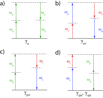
Figure 4: Energy diagrams representing the nonlinear optical processes included in Eqs. (92). (a) SPM and degenerate TPA corresponding to $\gamma_{\mu}^{\prime}$ and $\gamma_{\mu}^{\prime\prime}$, respectively. (b) XPM and XAM corresponding to $\gamma_{\mu\nu}^{\prime}$ and $\gamma_{\mu\nu}^{\prime\prime}$, respectively. Two possible ways of energy transfer that can occur during a degenerate FWM process: (c) two pump photons generate a signal and an idler photon, a process described by $\gamma_{psi}$; (d) the reverse process, described by $\gamma_{ips}$ and $\gamma_{spi}$, in which a signal and an idler photon generate two pump photons.

$$\bar{\kappa}_{\mu}(z)=\frac{\epsilon_{0}an^{2}}{2\bar{W}_{\mu}}\int_{S_{\mathrm{nl}}}|\mathbf{e}_{\mu}(\omega_{\mu})|^{2}dS,$$ (97a)

$$\gamma_{\mu}(z)=\frac{3\omega_{\mu}\epsilon_{0}a^{2}}{16v_{g,\mu}^{2}}\frac{1}{\bar{W}_{\mu}^{2}}\int_{S_{\mathrm{nl}}}\mathbf{e}_{\mu}^{*}(\omega_{\mu})$$

$$~{}~{}\cdot\hat{\chi}^{(3)}(\omega_{\mu},-\omega_{\mu},\omega_{\mu})\vdots\mathbf{e}_{\mu}(\omega_{\mu})\mathbf{e}_{\mu}^{*}(\omega_{\mu})\mathbf{e}_{\mu}(\omega_{\mu})dS,$$ (97b)

$$\gamma_{\mu\nu}(z)=\frac{3\omega_{\mu}\epsilon_{0}a^{2}}{16v_{g,\mu}v_{g,\nu}}\frac{1}{\bar{W}_{\mu}\bar{W}_{\nu}}\int_{S_{\mathrm{nl}}}\mathbf{e}_{\mu}^{*}(\omega_{\mu})$$

$$~{}~{}\cdot\hat{\chi}^{(3)}(\omega_{\nu},-\omega_{\nu},\omega_{\mu})\vdots\mathbf{e}_{\nu}(\omega_{\nu})\mathbf{e}_{\nu}^{*}(\omega_{\nu})\mathbf{e}_{\mu}(\omega_{\mu})dS,$$ (97c)

$$\gamma_{psi}(z)=\frac{3\omega_{p}\epsilon_{0}a^{2}}{16v_{g,p}{(v_{g,s}v_{g,i})}^{\frac{1}{2}}}\frac{1}{\bar{W}_{p}{(\bar{W}_{s}\bar{W}_{i})}^{\frac{1}{2}}}$$

$$~{}~{}\times\int_{S_{\mathrm{nl}}}\mathbf{e}_{p}^{*}(\omega_{p})\cdot\hat{\chi}^{(3)}(\omega_{s},-\omega_{p},\omega_{i})\vdots\mathbf{e}_{s}(\omega_{s})\mathbf{e}_{p}^{*}(\omega_{p})\mathbf{e}_{i}(\omega_{i})dS,$$ (97d)

$$\gamma_{spi}(z)=\frac{3\omega_{s}\epsilon_{0}a^{2}}{16v_{g,p}{(v_{g,s}v_{g,i})}^{\frac{1}{2}}}\frac{1}{\bar{W}_{p}{(\bar{W}_{s}\bar{W}_{i})}^{\frac{1}{2}}}$$

$$~{}~{}\times\int_{S_{\mathrm{nl}}}\mathbf{e}_{s}^{*}(\omega_{s})\cdot\hat{\chi}^{(3)}(\omega_{p},-\omega_{i},\omega_{p})\vdots\mathbf{e}_{p}(\omega_{p})\mathbf{e}_{i}^{*}(\omega_{i})\mathbf{e}_{p}(\omega_{p})dS,$$ (97e)

$$\gamma_{ips}(z)=\frac{3\omega_{i}\epsilon_{0}a^{2}}{16v_{g,p}{(v_{g,s}v_{g,i})}^{\frac{1}{2}}}\frac{1}{\bar{W}_{p}{(\bar{W}_{s}\bar{W}_{i})}^{\frac{1}{2}}}$$

$$~{}~{}\times\int_{S_{\mathrm{nl}}}\mathbf{e}_{i}^{*}(\omega_{i})\cdot\hat{\chi}^{(3)}(\omega_{p},-\omega_{s},\omega_{p})\vdots\mathbf{e}_{p}(\omega_{p})\mathbf{e}_{s}^{*}(\omega_{s})\mathbf{e}_{p}(\omega_{p})dS,$$ (97f)

where $\mu$ and $\nu\neq\mu$ take one of the values $p$, $s$, and $i$ and the frequency degeneracy at the pump frequency has been taken into account. Note that, as expected, when the nonlinear coefficients $\gamma$’s are real quantities, namely when nonlinear optical absorption effects can be neglected, the optical pumping term in Eq. (IV) vanishes. Moreover, since in experiments usually $P_{p}\gg P_{s},P_{i}$, the effective area given by Eq. (81) can be reduced to the following simplified form:

$$A_{\mathrm{nl}}(z)=\frac{\displaystyle\left(\int_{S_{\mathrm{nl}}}\big{|}\mathfrak{Re}\left[\mathbf{e}_{p}(\omega_{p})\times\mathbf{h}_{p}^{*}(\omega_{p})\right]\big{|}dS\right)^{2}}{\displaystyle\int_{S_{\mathrm{nl}}}\big{|}\mathfrak{Re}\left[\mathbf{e}_{p}(\omega_{p})\times\mathbf{h}_{p}^{*}(\omega_{p})\right]\big{|}^{2}dS}.$$ (98)

The types of nonlinear interactions incorporated in our theoretical model described by Eqs. (92) are summarized in Fig. 4 via the energy diagrams defined by the frequencies of the specific pairs of interacting photons. Thus, as per Fig. 4(a), the terms proportional to the $\gamma_{\mu}^{\prime}$ and $\gamma_{\mu}^{\prime\prime}$ coefficients describe SPM and degenerate TPA effects, respectively, whereas Fig. 4(b) illustrates XPM and XAM (also called nondegenerate TPA) interactions whose strength is proportional to $\gamma_{\mu\nu}^{\prime}$ and $\gamma_{\mu\nu}^{\prime\prime}$, respectively. Finally, there are two distinct types of FWM processes, represented in Fig. 4(c) and Fig. 4(d). In the first case two pump photons combine and generate a pair of photons, one at the signal frequency and the other one at the idler, a process described by the term proportional to $\gamma_{psi}$. The reverse process, represented by the $\gamma_{ips}$ and $\gamma_{spi}$ terms, corresponds to the case in which a signal and an idler photon combine to generate a pair of photons at the pump frequency.

As Eqs. (97) show, the linear and nonlinear optical coefficients of the waveguide depend on the index of refraction of silicon, both explicitly and implicitly via the optical modes of the waveguide. In our calculations the implicit modal frequency dispersion is not taken into account because it cannot be incorporated in the PWE method used to compute the modes. On the other hand, the explicit material dispersion is accounted for via the following Sellmeier equation describing the frequency dependence of the index of refraction of silicon p98book :

$$n^{2}(\lambda)=\epsilon+\frac{A}{\lambda^{2}}+\frac{B\lambda_{1}^{2}}{\lambda_{1}^{2}-\lambda^{2}},$$ (99)

where $\lambda_{1}=$1.1071\text{\,}\mathrm{\SIUnitSymbolMicro m}$$, $\epsilon=11.6858$, $A=$0.939\,816\text{\,}{\mathrm{\SIUnitSymbolMicro m}}^{2}$$, and $B=$8.104\,61\text{\times}{10}^{-3}$$.

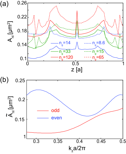
Figure 5: (a) Dependence of $A_{\mathrm{nl}}$ on $z$, determined for the odd (solid line) and even (dashed line) modes for several values of the group-index, $n_{g}$. (b) Frequency dispersion of $\tilde{A}_{\mathrm{nl}}$ calculated for the two modes, in the spectral domain where they are guiding modes.

The system of coupled equations, Eqs. (92) and Eq. (IV), form the basis for our analysis of degenerate FWM in silicon PhC waveguides. In our simulations, based on numerical integration of this system of equations using a standard split-step Fourier method combined with a fifth-order Runge-Kuta method for the integration of the linear, carriers dependent terms, the $z$-dependence of the coefficients in these equations is rigorously taken into account. However, one can significantly decrease the simulation time by averaging these fast-varying coefficients over a lattice constant, as this way the integration step for the resulting, averaged system can be increased considerably. The derivation of this averaged model is presented in the Appendix.

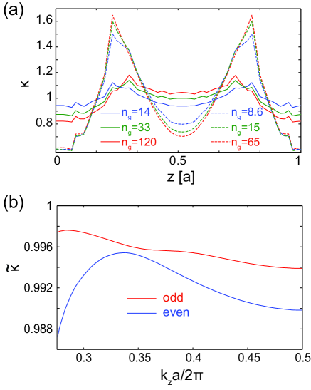
Figure 6: (a) Dependence of $\kappa$ on $z$, determined for the odd (solid line) and even (dashed line) modes for several values of the group-index, $n_{g}$. (b) Frequency dispersion of $\tilde{\kappa}$ calculated for the two modes, in the spectral domain where they are guiding modes.

One of the key differences between our theoretical description of FWM processes in Si-PhCWGs and the widely used models for FWM in waveguides with uniform cross-section, such as optical fibers or silicon photonic wires, is that the linear and nonlinear waveguide coefficients are periodic functions of the distance along the waveguide. In what follows, we discuss this feature of the FWM in more detail, starting with the effective area, $A_{\mathrm{nl}}$, defined by Eq. (98). The dependence of this area on the longitudinal distance, $z$, is presented in Fig. 5(a), where $z$ spans the length of a unit cell. As we have discussed, a physical characteristic of slow-light modes is their increased spatial extent. This property is clearly illustrated in Fig. 5(a), which shows that in the case of the even and odd modes the effective area increases by almost a factor of two when the group index varies from $14120$ and from $8.665$, respectively. This property is also illustrated by the frequency dispersion of the effective area, averaged over a unit cell, as per Fig. 5(b). Thus, it can be seen in this figure that the effective area has a maximum at $k_{z}\approx 0.3(2\pi/a)$ for the even mode and at the edge of the Brillouin zone for both modes, namely in the regions of slow light indeed.

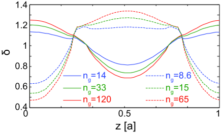
Figure 7: Dependence of $\delta$ on $z$, determined for several values of $n_{g}$. Solid and dashed lines correspond to the odd and even mode, respectively.

The $z$-dependence of the spatial mode overlap, $\kappa$, and the frequency dispersion of its spatial average over a unit cell, $\tilde{\kappa}$, are plotted in Figs. 6(a) and 6(b), respectively. These figures show that the mode overlap varies more strongly with $z$ in the case of the even mode, whereas in both cases the mode overlap variation increases as the group-index, $n_{g}$, increases. Interestingly enough, the averaged overlap coefficient of the even mode has a maximum at $k_{z}\approx 0.3(2\pi/a)$, i.e. $\lambda\approx$1.52\text{\,}\mathrm{\SIUnitSymbolMicro m}$$, which coincides with a minimum of its $v_{g}$. Note also that whereas $\kappa(z)$ can be larger than unity within the unit cell, its average, $\tilde{\kappa}<1$. This result is expected because $\tilde{\kappa}$ quantifies the mode overlap with the slab waveguide.

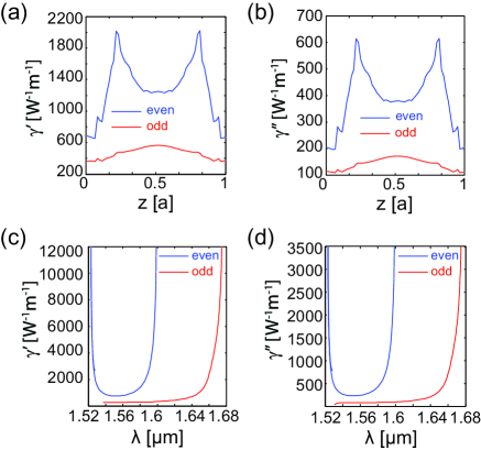
Figure 8: (a), (b) Dependence of $\gamma^{\prime}$ and $\gamma^{\prime\prime}$ on $z$, respectively, determined for $k_{z}=0.35(2\pi/a)$. (c), (d) Frequency dispersion of spatially averaged values of $\gamma^{\prime}(z)$ and $\gamma^{\prime\prime}(z)$, respectively, determined both for the even and odd modes.

In Fig. 7 we present the dependence on $z$ of another physical quantity that characterizes the linear optical properties of the PhC waveguide, namely its dispersive properties. This parameter, $\delta$, quantifies the extent to which the $z$-dependent dispersion coefficients differ from their averaged values. Similarly to the mode overlap coefficient $\kappa$, $\delta(z)$ shows a more substantial changes with $z$ in the case of the even mode as compared to the odd one and an increase of the amplitude of these oscillations with the increase of $n_{g}$. Moreover, as it has been demonstrated in the preceding section, the average of $\delta(z)$ over a unit cell is equal to unity.

The $z$-dependence of the nonlinear waveguide coefficient that characterizes the strength of SPM and TPA effects and the wavelength dependence of its average over a unit cell are plotted in the top and bottom panels of Fig. 8, respectively. One relevant result illustrated by these plots is that the nonlinear waveguide coefficient increases considerably as the GV of the optical mode is tuned to the slow-light regime. Indeed, for the case presented in Figs. 8(a) and 8(b) the group-index of the odd and even modes are $n_{g}=6.4$ and $n_{g}=11.5$, respectively. This phenomenon is better illustrated by the wavelength dependence of the spatially averaged values of $\gamma^{\prime}(z)$ and $\gamma^{\prime\prime}(z)$, which are shown in Figs. 8(c) and 8(d), respectively. Thus, these plots indicate that the nonlinear waveguide coefficient increases by more than an order of magnitude as the wavelength is tuned from the fast-light to the slow-light regime, the nonlinear interactions being enhanced correspondingly.

V Phase-matching condition

Before we use the theoretical model we developed to investigate the properties of FWM in Si-PhCWGs, we derive and discuss the conditions in which optimum nonlinear pulse interaction can be achieved. In particular, efficient FWM is achieved when the interacting pulses are phase-matched, namely when the total (linear plus nonlinear) wavevector mismatch is equal to zero. In the most general case this phase-matching condition depends in an intricate way on the peak power of the pump, $P_{p}$, signal, $P_{s}$, and idler, $P_{i}$, as well as on the linear and nonlinear coefficients of the waveguide a13book . This complicated relation takes a very simple form when one considers an experimental set-up most used in practice, namely when the pump is much stronger than the signal and idler, $P_{p}\gg P_{s},P_{i}$. Under these circumstances, the phase-matching condition can be expressed as:

$$2\gamma_{p}^{\prime}P_{p}-2\beta_{p}+\beta_{s}+\beta_{i}=0.$$ (100)

In order to determine the corresponding wavelengths of the optical pulses, this relation must be used in conjunction with the energy conservation relation, that is $2\omega_{p}=\omega_{s}+\omega_{i}$.

An alternative phase-matching condition, less accurate but easier to use in practice, can be derived by expanding the propagation constants, $\beta_{s,i}(\omega)$, in Taylor series around the pump frequency, $\omega_{p}$:

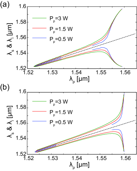
Figure 9: (a), (b) Wavelength diagrams defined by Eq. (100) and Eq. (102), respectively. In both panels dashed lines correspond to $\omega_{p}=\omega_{s}=\omega_{i}$.

$$\beta_{s,i}(\omega) =\sum_{n\geq 0}\frac{(\omega-\omega_{p})^{n}}{n!}\left.\frac{d^{n}\beta_{s,i}}{d\omega^{n}}\right|_{\omega=\omega_{p}}.$$ (101)

Inserting these expressions in Eq. (100) and neglecting all terms beyond the fourth-order, one arrives to the following relation:

$$2\gamma_{p}^{\prime}P_{p}+\beta_{2p}(\Delta\omega)^{2}+\frac{1}{12}\beta_{4p}(\Delta\omega)^{4}=0,$$ (102)

where $\Delta\omega\equiv|\omega_{p}-\omega_{s}|=|\omega_{p}-\omega_{i}|$.

The wavelength diagrams presented in Figs. 9(a) and 9(b) display the triplets of wavelengths for which the phase-matching conditions expressed by Eq. (100) and Eq. (102), respectively, are satisfied. These wavelength diagrams were calculated only for the even mode because only this mode possesses spectral regions with anomalous dispersion [cf. Fig. 3(b)], which is a prerequisite condition for phase-matching the FWM. More specifically, efficient FWM can be achieved if the pump wavelength ranges from $\lambda_{p}=$ $1.52\text{\,}\mathrm{\SIUnitSymbolMicro m}1.56\text{\,}\mathrm{\SIUnitSymbolMicro m}$. Moreover, the diagrams in Fig. 9 show that the predictions based on Eq. (100) and Eq. (102) are in good agreement, especially when $\Delta\omega$ is small. They start to agree less as $\Delta\omega$ increases because the contribution of the terms discarded when the series expansion of $\beta_{s,i}(\omega)$ is truncated increases as $\Delta\omega$ increases.

Figure 9 also suggests that the spectral domain in which efficient FWM is achieved depends on the pump power, $P_{p}$. To be more specific, it can be seen that for $P_{p}\lesssim$0.7\text{\,}\mathrm{W}$$, a spectral gap opens where the phase-matching condition cannot be satisfied. The spectral width of this gap increases when $P_{p}$ decreases as the the waveguide was not designed to possess phase-matched modes in the linear regime. Moreover, the diagrams presented in Fig. 9 show that in the fast-light regime the wavelengths defined by the phase-matching condition depend only slightly on $P_{p}$, whereas a much stronger dependence is observed when the wavelengths of the signal and idler lie in slow-light spectral domains.

VI Results and discussion

In this section we illustrate how our theoretical model can be used to investigate various phenomena related to FWM in Si-PhCWGs. In particular, we will compare the pulse interaction in slow- and fast-light regimes, calculate the FWM gain, and investigate the influence of various waveguide parameters on the FWM process. The choice of the values of physical parameters of the co-propagating pulses and that of the input pump power has been guided by the exact phase-matching condition given by Eq. (100). In all our calculations we assumed that the pulses propagate in the even mode and, unless otherwise specified, the following values for the pulse and waveguide parameters have been used in all our simulations: the input peak pump power, $P_{p}=10^{2}P_{s}=$5\text{\,}\mathrm{W}$$, the input pulse width, $T_{p}=T_{s}=$7\text{\,}\mathrm{ps}$$, and the intrinsic waveguide loss coefficient, $\alpha_{\mathrm{in}}=$50\text{\,}\mathrm{dB}\text{\,}{\mathrm{cm}}^{-1}$$.

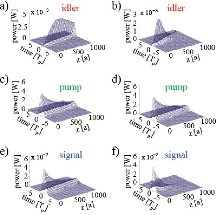
Figure 10: Pulse evolution in the time domain. Left (right) panels correspond to fast-light (slow-light) regimes, the group-index of the pulses being: $n_{g,i}=9.48$ ($n_{g,i}=20.3$), $n_{g,p}=8.64$ ($n_{g,p}=8.69$), $n_{g,s}=10.37$ ($n_{g,s}=23.3$).

Let us consider first the evolution of the envelopes of the pulses in the time domain, both in the slow- and fast-light regimes, as illustrated in Fig. 10. The triplet of wavelengths for which the phase-matching condition is satisfied is $\lambda_{p}=$1554\text{\,}\mathrm{nm}$$, $\lambda_{s}=$1536\text{\,}\mathrm{nm}$$, and $\lambda_{i}=$1571\text{\,}\mathrm{nm}$$ in the fast-light regime, whereas in the slow-light regime the wavelengths are $\lambda_{p}=$1559\text{\,}\mathrm{nm}$$, $\lambda_{s}=$1524\text{\,}\mathrm{nm}$$, and $\lambda_{i}=$1597\text{\,}\mathrm{nm}$$. We stress that in both cases the pump pulse propagates in the fast-light regime, whereas the signal and idler are both generated either in the fast- or slow-light regime.

Under these circumstances, one expects that the pump evolution in the time domain is similar in the two cases, a conclusion validated by the plots shown in Figs. 10(c) and 10(d). However, the dynamics of the signal and idler are strikingly different when they propagate in the slow-light or fast-light regimes. There are several reasons that account for these differences. First, whereas the FCA coefficient, $\alpha_{\mathrm{fc}}$, has similar values in the two cases, the FCA and intrinsic losses are much larger in the slow-light regime because the strength of both these effects is inverse proportional to $v_{g}$. This is reflected in Fig. 10 as a much more rapid decay in the slow-light regime of the signal and idler pulses. Second, it can be seen that in the slow-light regime the idler pulse grows at a faster rate. This is again a manifestation of slow-light effects. In particular, the nonlinear coefficient $\gamma_{ips}$, which determines the FWM gain, is inverse proportional to $(v_{g,i}v_{g,s})^{1/2}$ [see Eq. (97)]. As a consequence, the FWM gain is strongly enhanced when both the signal and idler propagate in the slow-light regime.

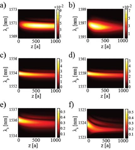
Figure 11: From top to bottom, the left (right) panels show the evolution of the spectra of the idler, pump, and signal in the case of fast-light (slow-light) regimes. The waveguide and pulse parameters are the same as in Fig. 10.

The slow-light effects are reflected not only in the characteristics of the time-domain propagation of the pulses but they also affect the evolution of the pulse spectra. In order to illustrate this idea, we plot in Fig. 11 the $z$-dependence of the spectra of the pulses. Similarly to the time-domain dynamics, the spectra of the pump are almost the same in the slow- and fast-light regimes as its GV does not differ much between the two cases. The most noteworthy differences between the slow- and fast-light scenarios can again be observed in the case of the idler and signal. Thus, in the slow-light regime the idler decays faster due to increased losses and grows and broadens more significantly because of enhanced FWM gain and FCD effects, respectively. The influence of FCD on the spectral features of the pulses can also be seen in the case of the signal and, to a smaller extent, the pump. More specifically, Eq. (9a) shows that the index of refraction of the waveguide decreases due to the generation of FCs. This in turn leads to a phase-shift and, consequently, a blue-shift of the pulse bkr04oe . Interestingly enough, one can also see in Fig. 11 that as the frequency of the pulses shifts during their propagation new spectral peaks are forming at the initial wavelengths for which the phase-matching condition was satisfied.

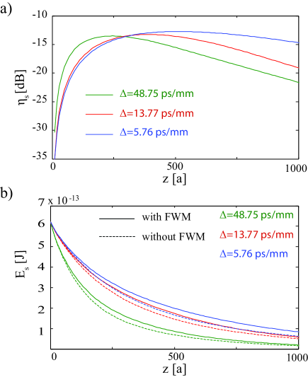
Figure 12: (a) FWM enhancement factor vs. propagation distance, determined for different values of the walk-off parameter, $\Delta=1/v_{g,s}-1/v_{g,p}$. (b) Signal energy vs. propagation distance, calculated by including FWM terms in Eqs. (92) and Eq. (IV) and by setting them to zero. The blue (green) curve corresponds to the fast-light (slow-light) regime considered in Fig. 10(a) [Fig. 10(b)], whereas the remaining triplet of phase-matched wavelengths is $\lambda_{p}=$1556\text{\,}\mathrm{nm}$$, $\lambda_{s}=$1530\text{\,}\mathrm{nm}$$, and $\lambda_{i}=$1582\text{\,}\mathrm{nm}$$ (red).

In order to gain a deeper insight into the influence of slow-light effects on the FWM process, we computed the $z$-dependence of the pulse energies when the frequencies of the signal and idler were tuned in the slow-light regions of the even mode of the waveguide. We considered two scenarios, namely these energies were calculated by including FWM terms in Eqs. (92) and Eq. (IV) and, in the other case, by setting them to zero, that is $\gamma_{psi}=\gamma_{spi}=\gamma_{ips}=0$. In the former case, the FWM terms are responsible for transferring energy from the pump pulse to the signal and idler. Therefore, a suitable quantity to characterize the efficiency of this energy transfer is what we call the FWM enhancement factor, $\eta$, which in the case of the signal is defined as $\eta_{s}=10\log[(E_{SXF}-E_{SX})/E_{s,in}]$. Here, $E_{SXF}$ and $E_{SX}$ are the signal energies calculated by taking into account, in one case, SPM, XPM, and FWM effects, and only SPM and XPM terms in the other case (i.e. FWM terms are neglected in the latter case), and $E_{s,in}$ is the input energy of the signal.

The results of these calculations are summarized in Fig. 12. In particular, it can be clearly seen in Fig. 12(a) that the FWM enhancement factor is strongly dependent on pulse propagation regime. To be more specific, as the signal and idler are shifting in the slow-light regime a smaller amount of energy is transferred from the pump pulse to the signal. There are two effects whose combined influence leads to this behavior. First, as we discussed, the pulses experience larger optical losses in the slow-light regime and therefore the signal losses energy at higher rate. Equally important, as the pulses are tuned in the slow-light regime the walk-off parameter, $\Delta$, defined as $\Delta=1/v_{g,s}-1/v_{g,p}$, increases, meaning that the pulses interact for a shorter time and consequently less energy is transferred to the signal. These conclusions are clearly validated by the results summarized in Fig. 12(b), where we plot the energy of the signal vs. the propagation distance, determined for several values of the walk-off parameter. In addition, this figure somewhat surprisingly suggests that the FWM process is more efficient in the fast-light regime, which is again due to the fact that the pump and signal overlap over longer time.

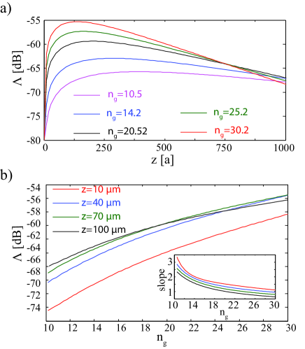
Figure 13: (a) Dependence of loss factor, $\Lambda$, on the propagation distance, $z$, determined for different values of the group-index, $n_{g}$. (b) Dependence of $\Lambda$ on $n_{g}$, determined for different values of $z$. The slopes of the curves corresponding to $z=$10\text{\,}\mathrm{\SIUnitSymbolMicro m}$$ and $z=$70\text{\,}\mathrm{\SIUnitSymbolMicro m}$$ are shown in the inset.

It is well known that in the slow-light regime linear optical effects are enhanced by a factor of $c/v_{g}$, whereas cubic nonlinear interactions increase by a factor of $(c/v_{g})^{2}$. For example, FCA and TPA are proportional to $v_{g}^{-1}$ and $v_{g}^{-2}$, respectively. Our theoretical model predicts, however, that when the mutual interaction between FCs and the optical field is taken into account these scaling laws can significantly change. This can be understood as follows: the amount of FCs generated via TPA, $N$, is proportional to $v_{g}^{-2}$ and since FCA is proportional to the product $v_{g}^{-1}N$, it scales with the GV as $v_{g}^{-3}$.

In order to validate this argument we have determined the optical total loss experienced by a pulse when it propagates in the presence of TPA and FCA or, in a different scenario, when only TPA is present [the latter case is realized by simply setting $\alpha_{\mathrm{fc}}=0$ in Eqs. (92)]. Moreover, to simplify our analysis, we consider the propagation of only one pulse by setting all parameters describing XPM and FWM interactions to zero. Finally, we also reduced the input power to $100\text{\,}\mathrm{mW}$ in order to avoid strong SPM-induced pulse reshaping. Under these conditions, the effect of the FCA on the pulse dynamics can be conveniently characterized by introducing a loss factor, $\Lambda$, defined as $\Lambda=10\log[(E_{T}-E_{TF})/E_{in}]$, where $E_{TF}$ and $E_{T}$ are the pulse energies in the case when both TPA and FCA terms are included in the model and when only TPA is present, respectively, and $E_{in}$ is the input energy of the pulse. The results of these calculations are presented in Fig. 13.

The variation of the loss factor, $\Lambda$, with the propagation distance, determined for several values of the GV is presented in Fig. 13(a). As one would have expected, the loss factor increases with the group-index, $n_{g}$, which is a reflection of the fact that the FC-induced losses increase with the decrease of the GV. One can observe, however, that when the propagation distance is larger than about $139a$ the loss factor begins to decrease when the GV decreases. This behavior is a direct manifestation of slow-light effects, namely as the frequency is tuned to the slow-light regime the optical losses increase significantly irrespective of the fact that only TPA is considered or both TPA and FCA effects are incorporated in the numerical simulations.

This subtle dependence of FC-induced losses on $v_{g}$ is perhaps better reflected by the plots presented in Fig. 13(b). Thus, for several values of the propagation distance, we have determined the variation of $\Lambda$ with the group-index, $n_{g}$. Then, by calculating the slope of the function $\Lambda(n_{g})$ represented on a logarithmic scale one can determine how FC-induced losses scale with $v_{g}$ [cf. the inset in Fig. 13(b)]. The results of this analysis clearly demonstrate that FC losses are proportional to $v_{g}^{-3}$, which agrees with the predictions of our qualitative evaluation of this dependence. We stress that for large $n_{g}$ (i.e., small $v_{g}$) the $v_{g}^{-3}$ dependence no longer holds at large propagation distance, chiefly because the pulse is strongly reshaped in the slow-light regime due to enhanced nonlinear optical effects, and thus its peak power is no longer exclusively determined by optical losses.

VII Conclusion

In conclusion, we have derived a rigorous theoretical model, which describes pulsed four-wave-mixing in one-dimensional photonic crystal slab waveguides made of silicon. Our theoretical model rigorously incorporate all key linear and nonlinear optical effects affecting the optical pulse dynamics, including modal dispersion, free-carrier dispersion, free-carrier absorption, self- and cross-phase modulation, two-photon absorption, cross-absorption modulation, and four-wave mixing. In addition, the mutual interaction between photogenerated free-carriers and optical field is incorporated in our theoretical analysis in a natural way by imposing the conservation the total energy of the optical field and free-carriers. Importantly, our theoretical formalism allows one to derive rigorous formulae for the optical coefficients characterizing the linear and nonlinear optical properties of the photonic crystal waveguides, avoiding thus any of the approximations that are commonly used in the investigation of nonlinear pulse dynamics in semiconductor waveguides based on photonic crystals.

As a practical application of the theoretical results developed in this study, we have used our theoretical model to investigate the properties of degenerate four-wave-mixing of optical pulses propagating in photonic crystal waveguides made of silicon, with a special focus being on highlighting the differences between the pulse dynamics in the slow- and fast light regimes. This analysis has revealed not only that linear and nonlinear effects are enhanced in the slow-light regime by a factor of $n_{g}$ and $n_{g}^{2}$, respectively, but also that these scaling laws are markedly affected in the presence of free-carriers. Moreover, since our study has been performed in a very general framework, i.e. generic optical properties of the waveguides (multi-mode waveguides) and pulse configuration (multi-frequency optical field), our findings can also be used to describe many phenomena not considered in this work. For example, important nonlinear effects, including stimulated and spontaneous Raman scattering, coherent anti-Stokes Raman scattering, and third-harmonic generation, can be included in our model by simply adding the proper nonlinear polarizations.

Appendix: Averaged model describing degenerate four-wave-mixing

The spatial scale over which the envelope of picosecond pulses varies is much larger than the lattice constant of the PhC and therefore for such optical pulses one can simplify the system of equations governing the pulse interaction, i.e. Eqs. (92) and Eq. (IV), by taking the average over one lattice constant. Under these conditions, the corresponding system of coupled equations can be cast in the following form:

$$i \bigg{(}\frac{\displaystyle\partial A_{p}}{\displaystyle\partial z}+\frac{1}{v_{g,p}}\frac{\partial A_{p}}{\partial t}\bigg{)}-\frac{\bar{\beta}_{2,p}}{2}\frac{\partial^{2}A_{p}}{\partial t^{2}}+\frac{\omega_{p}\delta n_{\mathrm{fc}}\tilde{\kappa}_{p}}{nv_{g,p}}A_{p}$$

$$+\frac{ic\tilde{\kappa}_{p}}{2nv_{g,p}}(\alpha_{\mathrm{fc}}+\alpha_{\mathrm{in}})A_{p}+2e^{i\Delta\bar{\beta}z}\tilde{\gamma}_{psi}A_{s}A_{i}A_{p}^{*}$$

$$+\left(\tilde{\gamma}_{p}|A_{p}{|}^{2}+2\tilde{\gamma}_{ps}|A_{s}{|}^{2}+2\tilde{\gamma}_{pi}|A_{i}{|}^{2}\right)A_{p}=0,$$ (103a)

$$i \bigg{(}\frac{\displaystyle\partial A_{s}}{\displaystyle\partial z}+\frac{1}{v_{g,s}}\frac{\partial A_{s}}{\partial t}\bigg{)}-\frac{\bar{\beta}_{2,s}}{2}\frac{\partial^{2}A_{s}}{\partial t^{2}}+\frac{\omega_{s}\delta n_{\mathrm{fc}}\tilde{\kappa}_{s}}{nv_{g,s}}A_{s}$$

$$+\frac{ic\tilde{\kappa}_{s}}{2nv_{g,s}}(\alpha_{\mathrm{fc}}+\alpha_{\mathrm{in}})A_{s}+e^{-i\Delta\bar{\beta}z}\tilde{\gamma}_{spi}A_{p}^{2}A_{i}^{*}$$

$$+\left(\tilde{\gamma}_{s}|A_{s}{|}^{2}+2\tilde{\gamma}_{sp}|A_{p}{|}^{2}+2\tilde{\gamma}_{si}|A_{i}{|}^{2}\right)A_{s}=0,$$ (103b)

$$i \bigg{(}\frac{\displaystyle\partial A_{i}}{\displaystyle\partial z}+\frac{1}{v_{g,i}}\frac{\partial A_{i}}{\partial t}\bigg{)}-\frac{\bar{\beta}_{2,i}}{2}\frac{\partial^{2}A_{i}}{\partial t^{2}}+\frac{\omega_{i}\delta n_{\mathrm{fc}}\tilde{\kappa}_{i}}{nv_{g,i}}A_{i}$$

$$+\frac{ic\tilde{\kappa}_{i}}{2nv_{g,i}}(\alpha_{\mathrm{fc}}+\alpha_{\mathrm{in}})A_{i}+e^{-i\Delta\bar{\beta}z}\tilde{\gamma}_{ips}A_{p}^{2}A_{s}^{*}$$

$$+\left(\tilde{\gamma}_{i}|A_{i}{|}^{2}+2\tilde{\gamma}_{ip}|A_{p}{|}^{2}+2\tilde{\gamma}_{is}|A_{s}{|}^{2}\right)A_{i}=0,$$ (103c)

$$\frac{\partial N}{\partial t}=-\frac{N}{\tau_{c}}+\frac{1}{\hbar}\bigg{\{}\sum_{\mu=p,s,i}\bigg{[}\frac{\Upsilon_{\mu}^{\prime\prime}}{\omega_{\mu}}|A_{\mu}{|}^{4}$$

$$~{}+\sum\limits_{\scriptsize{\begin{array}[]{c}\nu=p,s,i\\ \nu\neq\mu\end{array}}}\frac{4\Upsilon_{\mu\nu}^{\prime\prime}}{\omega_{\mu}+\omega_{\nu}}|A_{\mu}{|}^{2}|A_{\nu}{|}^{2}\bigg{]}+\frac{1}{\omega_{p}}\mathfrak{Im}\big{[}2\Upsilon_{psi}$$ (106)

$$~{}\times{A_{p}^{*}}^{2}A_{s}A_{i}e^{i\Delta\bar{\beta}z}+(\Upsilon_{spi}+\Upsilon_{ips})A_{p}^{2}A_{s}^{*}A_{i}^{*}e^{-i\Delta\bar{\beta}z}\big{]}\big{\}}.$$ (107)

The coefficients of the linear and nonlinear terms in these equations are given by the following formulae:

$$\tilde{\kappa}_{\mu}=\frac{\epsilon_{0}n^{2}}{2\bar{W}_{\mu}}\int_{V_{\mathrm{nl}}}|\mathbf{e}_{\mu}(\omega_{\mu})|^{2}dV,$$ (108a)

$$\tilde{\gamma}_{\mu}=\frac{3\omega_{\mu}\epsilon_{0}a}{16v_{g,\mu}^{2}}\frac{1}{\bar{W}_{\mu}^{2}}\int_{V_{\mathrm{nl}}}\mathbf{e}_{\mu}^{*}(\omega_{\mu})$$

$$~{}~{}\cdot\hat{\chi}^{(3)}(\omega_{\mu},-\omega_{\mu},\omega_{\mu})\vdots\mathbf{e}_{\mu}(\omega_{\mu})\mathbf{e}_{\mu}^{*}(\omega_{\mu})\mathbf{e}_{\mu}(\omega_{\mu})dV,$$ (108b)

$$\tilde{\gamma}_{\mu\nu}=\frac{3\omega_{\mu}\epsilon_{0}a}{16v_{g,\mu}v_{g,\nu}}\frac{1}{\bar{W}_{\mu}\bar{W}_{\nu}}\int_{V_{\mathrm{nl}}}\mathbf{e}_{\mu}^{*}(\omega_{\mu})$$

$$~{}~{}\cdot\hat{\chi}^{(3)}(\omega_{\nu},-\omega_{\nu},\omega_{\mu})\vdots\mathbf{e}_{\nu}(\omega_{\nu})\mathbf{e}_{\nu}^{*}(\omega_{\nu})\mathbf{e}_{\mu}(\omega_{\mu})dV,$$ (108c)

$$\tilde{\gamma}_{psi}=\frac{3\omega_{p}\epsilon_{0}a}{16v_{g,p}{(v_{g,s}v_{g,i})}^{\frac{1}{2}}}\frac{1}{\bar{W}_{p}{(\bar{W}_{s}\bar{W}_{i})}^{\frac{1}{2}}}$$

$$~{}~{}\times\int_{V_{\mathrm{nl}}}\mathbf{e}_{p}^{*}(\omega_{p})\cdot\hat{\chi}^{(3)}(\omega_{s},-\omega_{p},\omega_{i})\vdots\mathbf{e}_{s}(\omega_{s})\mathbf{e}_{p}^{*}(\omega_{p})\mathbf{e}_{i}(\omega_{i})dV,$$ (108d)

$$\tilde{\gamma}_{spi}=\frac{3\omega_{s}\epsilon_{0}a}{16v_{g,p}{(v_{g,s}v_{g,i})}^{\frac{1}{2}}}\frac{1}{\bar{W}_{p}{(\bar{W}_{s}\bar{W}_{i})}^{\frac{1}{2}}}$$

$$~{}~{}\times\int_{V_{\mathrm{nl}}}\mathbf{e}_{s}^{*}(\omega_{s})\cdot\hat{\chi}^{(3)}(\omega_{p},-\omega_{i},\omega_{p})\vdots\mathbf{e}_{p}(\omega_{p})\mathbf{e}_{i}^{*}(\omega_{i})\mathbf{e}_{p}(\omega_{p})dV,$$ (108e)

$$\tilde{\gamma}_{ips}=\frac{3\omega_{i}\epsilon_{0}a}{16v_{g,p}{(v_{g,s}v_{g,i})}^{\frac{1}{2}}}\frac{1}{\bar{W}_{p}{(\bar{W}_{s}\bar{W}_{i})}^{\frac{1}{2}}}$$

$$~{}~{}\times\int_{V_{\mathrm{nl}}}\mathbf{e}_{i}^{*}(\omega_{i})\cdot\hat{\chi}^{(3)}(\omega_{p},-\omega_{s},\omega_{p})\vdots\mathbf{e}_{p}(\omega_{p})\mathbf{e}_{s}^{*}(\omega_{s})\mathbf{e}_{p}(\omega_{p})dV,$$ (108f)

$$\Upsilon_{\varpi}=\frac{1}{a}\int_{z_{0}}^{z_{0}+a}\frac{\gamma_{\varpi}(z)}{A_{\mathrm{nl}}(z)}dz.$$ (108g)

where $V_{\mathrm{nl}}$ is the volume occupied by silicon in a unit cell of the PhC waveguide and $z_{0}$ an arbitrary distance. Finally, $A_{\mathrm{nl}}(z)$ in Eq. (108g) is given by Eq. (98), whereas the index $\varpi$ takes any of the following values: $p$, $s$, $i$, $ps$, $si$, $ip$, $psi$, $spi$, or $ips$.whereas the index $\varpi$ takes any of the following values: $p$, $s$, $i$, $ps$, $si$, $ip$, $psi$, $spi$, and $ips$. Note that in deriving the averaged equations governing the pulse and FC dynamics, Eqs. (103) and Eq. (Appendix: Averaged model describing degenerate four-wave-mixing), we have assumed that the FWM process is nearly phase-matched, namely $\Delta\bar{\beta}\ll 1/a$. In other words, the phase of the exponential factors in these equations vary much slower with the distance, $z$, as compared to the variation of the dielectric constant of the PhC waveguide.

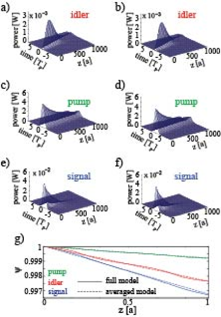
Figure 14: Comparison between pulse evolution as described by the full and averaged model is presented in the left and right panels, respectively. The group-index of the pulses are $n_{g,i}=20.3$, $n_{g,p}=8.69$, and $n_{g,s}=23.3$ and correspond to the slow-light propagation scenario presented in Fig. 10. The bottom panel shows the $z$-dependence of the normalized pulse amplitude, $\Psi_{\mu}(z)=A_{\mu}(z_{0}+z)/A_{\mu}(z_{0})$, $\mu=p,s,i$, calculated for the unit cell starting at $z_{0}=200a$.

A comparison between the predictions of the full and averaged models is illustrated in Fig. 14. Thus, we have considered the slow-light pulse dynamics presented in Fig. 10 and determined the pulse evolution using both the full and averaged models. As it can be seen, both models predict a similar pulse dynamics for the entire propagation length, $z=1000a$. This result is expected as the envelope of picosecond pulses, as are those chosen in our simulations, spans a large number of unit cells and therefore the pulse amplitude is only slightly affected by the local inhomogeneity of the index of refraction.

The fast variation with $z$ of the pulse envelope is shown in Fig. 14(g), where we plot the $z$-dependence of the normalized pulse amplitude, $\Psi_{\mu}(z)=A_{\mu}(z_{0}+z)/A_{\mu}(z_{0})$, $\mu=p,s,i$, calculated for the unit cell starting at $z_{0}=200a$. It can be seen in this figure that the pulse envelope varies at a spatial scale commensurable with the lattice constant yet the amplitude of these variations is much smaller than the pulse peak amplitude. The magnitude of these variations, however, would comparatively become more significant should the pulse duration would be brought to the femtosecond range.

References

- (1) R. Ho, K. W. Mai, and M. A. Horowitz, Proc. IEEE 89, 490 (2001).
- (2) K. K. Lee, D. R. Lim, H. C. Luan, A. Agarwal, J. Foresi, and L. C. Kimerling, Appl. Phys. Lett. 77, 1617 (2000).
- (3) R. U. Ahmad, F. Pizzuto, G. S. Camarda, R. L. Espinola, H. Rao, and R. M. Osgood, IEEE Photon. Technol. Lett. 14, 65 (2002).
- (4) R. Claps, D. Dimitropoulos, V. Raghunathan, Y. Han, and B. Jalali, Opt. Express 11, 1731 (2003).
- (5) R. Espinola, J. I. Dadap, R. M. Osgood, S. J. McNab, and Y. A. Vlasov, Opt. Express 12, 3713 (2004).
- (6) H. S. Rong, R. Jones, A. S. Liu, O. Cohen, D. Hak, A. Fang, and M. Paniccia, Nature (London) 433, 725 (2005).
- (7) M. A. Foster, A. C. Turner, J. E. Sharping, B. S. Schmidt, M. Lipson, and A. L. Gaeta, Nature (London) 441, 960 (2006).
- (8) X. Liu, R. M. Osgood, Y. A. Vlasov, and W. M. J. Green, Nat. Photonics 4, 557 (2010).
- (9) G. Cocorullo, M. Iodice, I. Rendina, and P. M. Sarro, IEEE Photon. Technol. Lett. 7, 363 (1995).
- (10) A. Liu, R. Jones, L. Liao, D. Samara-Rubio, D. Rubin, O. Cohen, R. Nicolaescu, and M. Paniccia, Nature (London) 427, 615 (2004).
- (11) Q. Xu, B. Shmidt, S. Pradhan, and M. Lipson, Nature (London) 435, 325 (2005).
- (12) X. Chen, N. C. Panoiu, I. W. Hsieh, J. I. Dadap, and R. M. Osgood, IEEE Photon. Technol. Lett. 18, 2617 (2006).
- (13) M. Mohebbi, IEEE Photon. Technol. Lett. 20, 921 (2008).
- (14) O. Boyraz, P. Koonath, V. Raghunathan, and B. Jalali, Opt. Express 12, 4094 (2004).
- (15) I. W. Hsieh, X. Chen, X. P. Liu, J. I. Dadap, N. C. Panoiu, C. Y. Chou, F. Xia, W. M. Green, Y. A. Vlasov, and R. M. Osgood, Opt. Express 15, 15242 (2007).
- (16) N. C. Panoiu, X. Liu, and R. M. Osgood, Opt. Lett. 34, 947 (2009).
- (17) N. C. Panoiu, X. Chen, and R. M. Osgood, Opt. Lett. 31, 3609 (2006).
- (18) H. Fukuda, K. Yamada, T. Shoji, M. Takahashi, T. Tsuchizawa, T. Watanabe, J. Takahashi, and S. Itabashi, Opt. Express 13, 4629 (2005).
- (19) R. Espinola, J. Dadap, R. M. Osgood, S. McNab, and Y. Vlasov, Opt. Express 13, 4341 (2005).
- (20) M. A. Foster, A. C. Turner, R. Salem, M. Lipson, and A. L. Gaeta, Opt. Express 15, 12949 (2007).
- (21) S. Zlatanovic, J. S. Park, S. Moro, J. M. C. Boggio, I. B. Divliansky, N. Alic, S. Mookherjea, and S. Radic, Nat. Photonics 4, 561 (2010).
- (22) J. B. Driscoll, N. Ophir, R. R. Grote, J. I. Dadap, N. C. Panoiu, K. Bergman, and R. M. Osgood, Opt. Express 20, 9227 (2012).
- (23) R. M. Osgood, N. C. Panoiu, J. I. Dadap, X. Liu, X. Chen, I-W. Hsieh, E. Dulkeith, W. M. J. Green, and Y. A. Vlassov, Adv. Opt. Photon. 1, 162 (2009).
- (24) E. Yablonovitch, Phys. Rev. Lett. 58, 2059 (1987).
- (25) S. John, Phys. Rev. Lett. 58, 2486 (1987).
- (26) A. Mekis, J. C. Chen, I. Kurland, S. Fan, P. R. Villeneuve, and J. D. Joannopoulos, Phys. Rev. Lett. 77, 3787 (1996).
- (27) S. Y. Lin, E. Chow, V. Hietala, P. R. Villeneuve, J. D. Joannopoulos, Science 282, 274 (1998).
- (28) T. Baba, N. Fukaya, and J. Yonekura, Electron. Lett. 35, 654 (1999).
- (29) S. G. Johnson, S. Fan, P. R. Villeneuve, J. D. Joannopoulos, and L. A. Kolodziejski, Phys. Rev. B 60, 5751 (1999).
- (30) A. Chutinan and S. Noda, Phys. Rev. B 62, 4488 (2000).
- (31) J. S. Foresi, P. R. Villeneuve, J. Ferrera, E. R. Thoen, G. Steinmeyer, S. Fan, J. D. Joannopoulos, L. C. Kimerling, H. I. Smith, and E. P. Ippen, Nature (London) 390, 143 (1997).
- (32) O. Painter, R. K. Lee, A. Scherer, A. Yariv, J. D. O’Brien, P. D. Dapkus, and I. Kim, Science 284, 1819 (1999).
- (33) Y. Akahane, T. Asano, B. S. Song, and S. Noda, Nature (London) 425, 944 (2003).
- (34) J. P. Reithmaier, G. Sek, A. Loffler, C. Hofmann, S. Kuhn, S. Reitzenstein, L. V. Keldysh, V. D. Kulakovskii, T. L. Reinecke, and A. Forchel, Nature (London) 432, 197 (2004).
- (35) T. Yoshie, A. Scherer, J. Hendrickson, G. Khitrova, H. M. Gibbs, G. Rupper, C. Ell, O. B. Shchekin, and D. G. Deppe, Nature (London) 432, 200 (2004).
- (36) S. Fan, P. R. Villeneuve, J. D. Joannopoulos, M. J. Khan, C. Manolatou, and H. A. Haus, Phys. Rev. B 59, 15882 (1999).
- (37) A. Chutinan, M. Mochizuki, M. Imada, and S. Noda, Appl. Phys. Lett. 79, 2690 (2001).
- (38) M. Soljacic and J. D. Joannopoulos, Nat. Mater. 3, 211 (2004).
- (39) T. F. Krauss, Nat. Photonics 2, 448 (2008).
- (40) T. Baba, Nat. Photonics 2, 465 (2008).
- (41) M. Notomi, K. Yamada, A. Shinya, J. Takahashi, C. Takahashi, and I. Yokohama, Phys. Rev. Lett. 87, 253902 (2001).
- (42) M. Soljacic, S. G. Johnson, S. Fan, M. Ibanescu, E. Ippen, and J. D. Joanopoulos, J. Opt. Soc. Am. B 19, 2052 (2002).
- (43) N. C. Panoiu, M. Bahl, and R. M. Osgood, Opt. Lett. 28, 2503 (2003).
- (44) N. C. Panoiu, M. Bahl, and R. M. Osgood, Opt. Express 12, 1605 (2004).
- (45) Y. A. Vlasov, M. O. Boyle, H. F. Hamann, and S. J. McNab, Nature (London) 438, 65 (2005).
- (46) J. F. McMillan, X. Yang, N. C. Panoiu, R. M. Osgood, and C. W. Wong, Opt. Lett. 31, 1235 (2006).
- (47) B. Corcoran, C. Monat, C. Grillet, D. J. Moss, B. J. Eggleton, T. P. White, L. O’Faolain, and T. F. Krauss, Nat. Photonics 3, 2503 (2009).
- (48) I. H. Rey, Y. Lefevre, S. A. Schulz, N. Vermeulen, and T. F. Krauss, Phys. Rev. B 84, 035306 (2011).
- (49) J. F. McMillan, M. Yu, D. L. Kwong, and C. W. Wong, Opt. Express 18, 15484 (2010).
- (50) M. Santagiustina, C. G. Someda, G. Vadala, S. Combrie, and A. De Rossi, Opt. Express 18, 21024 (2010).
- (51) C. Monat, M. Ebnali-Heidari, C. Grillet, B. Corcoran, B. J Eggleton, T. P. White, L. O’Faolain, J. Li, and T. F. Krauss, Opt. Express 18, 22915 (2010).
- (52) J. Li, L. O’Faolain, I. H. Rey, and T. F. Krauss, Opt. Express 19, 4458 (2011).
- (53) T. Chen, J. Sun, and L. Li, Opt. Express 20, 20043 (2012).
- (54) S. Lavdas, S. Zhao, J. B. Driscoll, R. R. Grote, R. M. Osgood, and N. C. Panoiu, Opt. Lett. 39, 401 (2014).
- (55) J. D. Joannopoulos, S. G. Johnson, J. N. Winn, and R. D. Meade, Photonic Crystals: Molding the Flow of Light, 2nd ed. (Princeton University Press, Princeton, NJ, 2008).
- (56) S. G. Johnson and J. D. Joannopoulos, Opt. Express 8, 173 (2001).
- (57) X. Chen, N. C. Panoiu, and R. M. Osgood, IEEE J. Quantum Electron. 42, 160 (2006).
- (58) N. C. Panoiu, J. F. McMillan, and C. W. Wong, IEEE J. Sel. Top. Quantum Electron. 16, 257 (2010).
- (59) A. W. Snyder, IEEE Trans. Microw. Theory Tech. 18, 383 (1970).
- (60) J. E. Sipe, C. M. de Sterke, and B. J. Eggleton, J. Mod. Opt. 49, 1437 (2002).
- (61) R. A. Soref and B. R. Bennett, IEEE J. Quantum Electron. 23, 123 (1987).
- (62) R. W. Boyd, Nonlinear Optics, 3rd ed. (Academic Press, San Diego, 2008).
- (63) J. Zhang, Q. Lin, G. Piredda, R. W. Boyd, G. P. Agrawal, and P. M. Fauchet, Appl. Phys. Lett. 91, 071113(1-3) (2007).
- (64) D. Michaelis, U. Peschel, C. Wachter, and A. Brauer, Phys. Rev. E 68, 065601(R)(1-4) (2003).
- (65) T. Kamalakis and T. Sphicopoulos, IEEE J. Quantum Electron. 43, 923 (2007).
- (66) A. W. Snyder and J. D. Love, Optical Waveguide Theory (Chapman and Hall, London, 1983).
- (67) P. N. Butcher and D. Cotter, The Elements of Nonlinear Optics (Cambridge University Press, 1991).
- (68) C. Monat, B. Corcoran, M. Ebnali-Heidari, C. Grillet, B. J. Eggleton, T. P. White, L. O’Faolain, and T. F. Krauss, Opt. Express 17, 2944 (2009).
- (69) E. D. Palik, Handbook of Optical Constants of Solids (Academic Press, San Diego, 1998).
- (70) G. P. Agrawal, Nonlinear Fiber Optics, 5th ed. (Academic Press, San Diego, 2013).