Dynamics of social contagions with memory of non-redundant information

Abstract

A key ingredient in social contagion dynamics is reinforcement, as adopting a certain social behavior requires verification of its credibility and legitimacy. Memory of non-redundant information plays an important role in reinforcement, which so far has eluded theoretical analysis. We first propose a general social contagion model with reinforcement derived from non-redundant information memory. Then, we develop a unified edge-based compartmental theory to analyze this model, and a remarkable agreement with numerics is obtained on some specific models. Using a spreading threshold model as a specific example to understand the memory effect, in which each individual adopts a social behavior only when the cumulative pieces of information that the individual received from his/her neighbors exceeds an adoption threshold. Through analysis and numerical simulations, we find that the memory characteristic markedly affects the dynamics as quantified by the final adoption size. Strikingly, we uncover a transition phenomenon in which the dependence of the final adoption size on some key parameters, such as the transmission probability, can change from being discontinuous to being continuous. The transition can be triggered by proper parameters and structural perturbations to the system, such as decreasing individuals’ adoption threshold, increasing initial seed size, or enhancing the network heterogeneity.

I Introduction

Due to technological advances social networks are playing an ever increasing role in the modern society. In a social network, nodes are individuals of the population while links represent the social ties or relations among individuals Castellano2009 . In recent years, there is a growing interest in investigating the phenomenon of behavior spreading on social networks, where the behaviors range from adoption of an innovation Young2011 and healthy activities Centola2011 to microfinance Banerjee2013 . This is essentially the problem of social contagion. Ample experimental and theoretical results indicated that, unlike biological contagions in which successive contacts result in contagion with independent probabilities, in a social contagion the probability of infection depends on previous contacts. This is equivalent to social affirmation or reinforcement effect, since multiple confirmation of the credibility and legitimacy of the behavior is always sought Centola2007 ; Dodds2004 ; Dodds2005 ; Centola2010 ; Weiss2014 . For an individual, who had two friends adopting a particular behavior before a given time and whose third friend newly adopts the behavior, whether he/she adopts this behavior will take the three friends into account.

An early mathematical model to describe the dynamics of social contagions is the threshold model Granovetter1973 ; Watts2002 based on Markovian process without memory, in which adoption of behaviors depends only on the states of the current active neighbors (i.e., individuals who have adopted the behavior), and an individual adopts a behavior only when the current number or the fraction of his/her active neighbors is equal to or exceeds some adoption threshold. Analytically, the fraction of individuals adopting the behavior eventually, can be predicted using the percolation theory Watts2002 for situations where the initial seed size is vanishingly small. One result is that, for a fixed threshold, as the mean degree is increased, the final size tends to grow continuously and then decrease discontinuously. As the degree distribution becomes more heterogeneous, the network is less vulnerable to social contagions, in sharp contrast to the dynamics of epidemic spreading Newman2002 ; Pastor-Satorras2001 ; Boguna2013 ; Castellano2010 . Previous research also revealed that, within the threshold model, factors such as the initial seed size Gleeson2007 , clustering coefficient Whitney2010 , community structure Gleeson2008 ; Nematzadeh2014 , multiplexity Yagan2013 ; Brummitt2012 ; Lee2014 , and temporal networks Takaguchi2013 ; Karimi2013 all can affect the social contagion process.

In real situations of social contagions, memory typically plays an important role in the adoption and reinforcement of behaviors, which includes full Centola2011 or partial Dodds2004 memory of the cumulative behavioral information (behavioral information can be referred as information for short) that individuals received from their neighbors. This memory effect makes the dynamics of social contagions have non-Markovian characteristic. To account for the memory effect, sophisticated non-Markovian models were proposed Lv2011 ; Centola2011 ; Dodds2004 ; Dodds2005 ; Chung2014 ; Aral2012 ; Banerjee2013 . In some models, it was predicted that the final adoption size will grow discontinuously Dodds2004 ; Dodds2005 ; Chung2014 , if the adoption probability for an individual who receives more than one piece of information is two times larger than the adoption probability for individuals getting only one piece of information. In general, the memory of cumulative information about the particular social behavior can come from redundant Dodds2004 ; Dodds2005 or non-redundant Watts2002 information transmission, where the former allows a pair of individuals to transmit information successfully more than once but for the latter, repetitive transmission is forbidden. In some social contagion processes such as risk migration and use of unproven technologies Centola2007 , transmitting redundant information between the same pair of individuals is unnecessary, since each neighbor can guarantee the credibility and legitimacy of the behavior but only to certain extent Centola2011 . However, such non-redundant information transmission characteristic of social reinforcement have essentially been neglected in previous studies Dodds2004 ; Dodds2005 .

A systematic study to understand the effects of non-redundant information memory on social contagion dynamics is thus called for. A general model needs to include different situations of behavior adoption such as the dependence of the adoption probability on non-redundant information Centola2011 or even on the structure diversity of such information Ugander2012 . Due to the non-Markovian nature of the memory characteristic, to develop a general theory is challenging. Some approximate approaches were devised such as those based on mean field analysis Dodds2004 , percolation theory Chung2014 , and renewal process Mieghem2013 ; Cator2013 . Since the non-Markovian property induces strong dynamical correlations between any two connected individuals, analytic predictions from these approaches tend to deviate significantly from results from direct numerical simulations, especially when the underlying network is strongly structurally heterogeneous Pastor-Satorras2014 .

In this paper, we articulate a general social contagion model with social reinforcement derived from memory of non-redundant information to address the general question of how behaviors spread on networks in a more systematic and complete way. In order to understand, quantitatively, the effects of this kind of memory characteristic on social contagion dynamics, we develop a unified edge-based compartmental theory. We base our study on the spreading threshold model, focusing on the final behavior adoption size and its dependence on the transmission probability under different dynamical and topological parameter settings. We find that the memory characteristic generally have a strong effect on the final adoption size. Surprisingly, we uncover a crossover between discontinuous and continuous variations in the final adoption size. More specifically, the crossover phenomenon can be induced by decreasing individuals’ adoption threshold, increasing the initial seed size or enhancing the structural heterogeneity of the network. Our theoretical predictions agree well with results from numerical simulations. We further generalize our theory to treat distinct social contagion models and network structures.

In Sec. II, we describe our general social contagion model with reinforcement derived from memory of non-redundant information on complex networks. In Sec. III, we detail our edge-based compartmental theory and analysis. In Sec. IV, we present results from extensive numerical computations to validate our theory. In Sec. V, we extend our theoretical framework to analyze alternative social contagion models, demonstrating the generality of our theory. In Sec. VI, we present conclusions and discussions.

II A General Social Contagion Model

Our goal is to construct a general stochastic model for social contagion dynamics, taking into account social reinforcement through non-redundant information memory characteristic. In this model, information refers to the behavioral information. The non-redundant information memory has two features: (1) non-redundant information transmission, i.e., repetitive information transmission on every edge is forbidden, and thus also can be called as single-transmission; (2) every individual can remember the cumulative pieces of non-redundant information that the individual received from his/her neighbors, which makes the contagion processes be non-Markovian.

Concretely, we consider a configuration network model Catanzaro2005 of size $N$ and degree distribution $P(k)$, where nodes in the network represent individuals. There is no degree-degree correlations when the network is very large and sparse. At any time, each individual can exist in one of the three different states: susceptible, adopted, or recovered. In the susceptible state, an individual does not adopt the social behavior. In the adopted state, an individual adopts the behavior and transmits the behavioral information to his/her neighbors. In the recovered state, an individual loses interest in the behavior and will not spread the information further. This is thus a susceptible-adopted-recovered (SAR) model. Although this proposed model has similar state definitions with the epidemiology susceptible - infected - recovered (SIR) model Newman2002 , the non-markovian characteristic is absent in the SIR model.

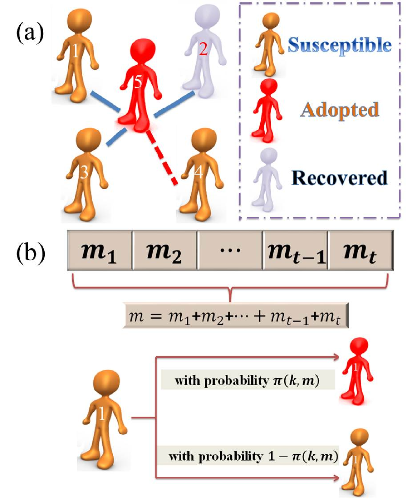
Figure 1: (Color online) Illustration of the susceptible-adopted-recovered (SAR) model on complex networks. (a) At time $t$, the adopted individual $5$ tries to transmit the behavioral information (or simply information for short) to each susceptible neighbor individual independently with probability $\lambda$. Note that individual $5$ can not transmit the information to individual $4$, since he/she has transmitted the information to individual $4$ successfully before time $t$. That is to say, the susceptible individual can only get the non-redundant information from his/her neighbors. The solid blue lines denote that the information has not transmitted through them successfully, and the red dished line denotes that the information has transmitted through it previously. (b) Assuming that individual $1$ has received a new piece of information at time $t$, whether individual $1$ adopts the behavior is determined by the $m$ cumulative pieces of information he/she ever received from neighbors. The value of $m$ can be expressed as $m=\sum_{d=1}^{t}m_{d}$, where $m_{d}$ is the pieces of information that individual $1$ received at time $d$. In such a situation, individual $1$ has to remember the pieces of non-redundant information he/she received from neighbors before time $t$. Thus, the so called non-redundant information memory is induced. Individual $1$ becomes adopted with probability $\pi(k,m)$, where $k$ is the degree of individual $1$; otherwise, individual $1$ remains in the susceptible state.

To initiate a social contagion, a fraction $\rho_{0}$ of individuals are uniformly randomly chosen to be in the adopted state and the remaining majority of the individuals are in the susceptible state. At each time step, behavioral information propagates from each adopted individual to each neighbor independently with transmission probability $\lambda$, a key parameter of the underlying dynamical process. We assume an edge that has transmitted the information successfully will never transmit the same information again, i.e., non-redundant information transmission. The non-redundant information spreading process is illustrated schematically in Fig. 1(a). Based on this setting, we introduce the memory effect of non-redundant information in social reinforcement. In particular, assume that a susceptible individual $u$ of degree $k$ already has $m-1$ pieces of information from distinct neighbors. Once $u$ is successfully informed of the social behavior by one of his/her adopted neighbors, denoted as $v$, the cumulative number of pieces of information that $u$ has will increase by $1$. With the $m$ cumulative pieces of information up to now (i.e., after exposing to $m$ pieces of non-redundant information), the probability that the individual will be in the adopted state is $\pi(k,m)$. Note that $u$ may subsequently get more than one pieces of information successfully in this time step, thus, he/she will try to adopt the behavior when he/she gets every new piece of information. In this case, if $u$ gets the $(n+1)$th new information in this step, he/she will adopt the behavior with probability $\pi(k,m+n)$. An illustration of the behavior adoption process is presented in Fig. 1(b). Since $\pi(k,m)<1$ in general, multiple information transmission is necessary for $u$ to move into the adopted state, thereby incorporating the memory characteristic into the model. Generally, $\pi(k,m)$ is a monotonically increasing function of $m$ for any given degree $k$, which characterizes the reinforcement effect through non-redundant information memory. If $\pi(k,m)$ is a constant, no such reinforcement effect exists. In this case, if the adopted state is regarded as the infected state in epidemiology, our model will reduce to the standard SIR (susceptible - infected - recovered) model Newman2002 , where social reinforcement effect and non-Markovian properties are not present - a key difference between biological and social contagions. Empirical researches indicate that the adopted individuals may lose interest in the behavior Karsai2014 , which is also concerned in the binary social dynamics Dodds2013 ; Harris2013 . At the same time step, we thus assume that each adopted individual loses interest in transmitting the behavioral information and becomes recovered with probability $\gamma$. The spreading dynamics terminates once all adopted individuals have become recovered.

By setting the parameters, our stochastic model can generate either Markovian or non-Markovian processes, thereby including a number of existing models on social contagions as different limiting cases. For example, if $\pi(k,m)$ is a Heaviside step function (i.e., if $m$ is less than the adoption threshold $T_{u}$, then $\pi$ is zero; otherwise, $\pi$ is unity), and setting $\lambda=1.0$ and $\gamma=0.0$, we obtain the Watts threshold model Watts2002 . Once the thresholds of individuals and network topology are fixed, the cascade process in the Watts threshold model will be deterministic, which is a trivial case of Markovian process. In addition, by choosing the dynamical parameters properly, we can map our model into some of the existing non-Markovian models. For instance, fixing $\lambda=1.0$ and letting $\pi(k,m)$ be a function of exactly one of the two quantities (i.e., adopted and susceptible individuals), we recover the synergy spreading model Francisco2011 . Similarly, if we allow $\pi(k,m)$ to be a linear Chung2014 or exponential Lv2011 function of $m$ and $\gamma=1.0$, we can obtain distinct types of non-Markovian dynamics. Differing from the models in Refs. Chung2014 ; Lv2011 in which each adopted individual only gets one chance to transmit the behavioral information to every neighbor, in our model an adopted individual can try to transmit the information many times until he/she becomes recovered state or transmits the information successfully.

In our study, we concentrate on the so-called spreading threshold model before turning to more generalized social contagion models. In the spreading threshold model, an individual $u$ adopts the behavior only when the number of pieces of non-redundant information that $u$ possessed exceeds the adoption threshold $T_{u}$. This means that the adoption probability $\pi(k,m)$ is a Heaviside step function, which has the same form as in the Watts threshold model Watts2002 . There are, however, key differences between the two types of threshold models. Firstly, differing from the Watts model in which the adoption threshold is the corresponding fraction of neighboring nodes, the adoption threshold in our model is expressed in terms of the absolute number of neighboring nodes, as in bootstrap percolation Baxter2010 and self-organized criticality models Zhang1989 . Secondly, in the Watts model, each individual can obtain information about the states of all its neighbors “instantaneously” at each time step, but in our model individuals are able to know the neighboring states only through transmission of the information. Thirdly, in the Watts model an individual is permanently interested in the behavior even after its adoption, while we assume more realistically that individuals having adopted certain behavior may lose interest in it and never spread the corresponding information, which is quantified by the abandon probability $\gamma$. Note that if the threshold of Watts model is expressed as the absolute number of neighbors who have adopted the behavior, there will only exist the second and third differences. These three differences are consequences of introducing the non-redundant information memory characteristic into our model, better capturing the essential dynamics of social contagions in the real world.

III Theory

We first develop a unified edge-based compartmental theory to analyze our general social contagion model with reinforcement mechanism based on non-redundant information memory characteristic. We then systematically investigate how the memory affects the social contagion process in a specific model, the spreading threshold model. In this theory, we assume that the networks have large network sizes, sparse edges, and no degree-degree correlations, and the contagion dynamics evolves continuously. Mathematically, a contagion process can be described by three variables: $S(t)$, $A(t)$ and $R(t)$, which are the densities of the susceptible, adopted, and recovered individuals at time $t$, respectively. The states of all individuals remain unchanged when $t\to\infty$, and $R(\infty)$ is the final fraction of individuals that have adopted the social behavior.

III.1 General theoretical framework

Due to the non-redundant information memory characteristic, in a social contagion process there are strong dynamical correlations between the states of the adjacent nodes, making existing theoretical methods such as the mean-field theory Dodds2004 , percolation theory Gleeson2007 , and renewal process Cator2013 inapplicable, especially for networks that are strongly structurally heterogeneous. Using insights from Refs. Miller2011 ; Miller2013 ; Wang2014A ; Valdez2012 , we develop an edge-based compartmental theory to analyze social contagion dynamics in the presence of strong nodal state correlations.

Let $\theta(t)$ be the probability that individual $v$ has not transmitted the information to individual $u$ along a randomly chosen edge by time $t$. In the spirit of the cavity theory Karrer2010 ; Miller2013 , we disallow individual $u$ to transmit any information to its neighbors but $u$ can receive such information from its neighbors - $u$ is in a cavity state. Initially, a fraction of $\rho_{0}$ individuals is in the adopted state, and none of them transmits the information to its neighbors, so $\theta(0)=1$ for all edges. For simplicity in theory, we assume that the probability of not transmitting the information is identical for all edges, and dynamical correlations doesn’t exist among neighbors of an individual. At time $t$, a uniformly randomly chosen individual $u$ of degree $k$ in the cavity state has been exposed to $m$ pieces of non-redundant information (i.e., $u$ has received the information from distinct neighbors $m$ times) with the probability

$$\phi_{m}(k,\theta(t))=(1-\rho_{0})\binom{k}{m}\theta(t)^{k-m}[1-\theta(t)]^{m},$$ (1)

where the factor $(1-\rho_{0})$ is the fraction of susceptible nodes initial. By time $t$, the susceptible individual $u$ has received the information from $m$ different neighbors. The probability that $u$ has not adopted the behavior for time of receiving information less than $m$ is $\Pi_{j=0}^{m}[1-\pi(k,j)]$. Combining this factor and summing over all possible values of $m$, we obtain the probability that the individual $u$ is still in the susceptible state at time $t$ as

$$s(k,t)=\sum_{m=0}^{k}\phi_{m}(k,t)\Pi_{j=0}^{m}[1-\pi(k,j)].$$ (2)

Taking into account different degrees in the network, we obtain the fraction of susceptible individuals (i.e., the probability of a randomly chosen individual is in the susceptible state) at time $t$ as

$$S(t)=\sum_{k=0}^{\infty}P(k)s(k,t).$$ (3)

Analogously, the fraction of individuals with $m$ pieces of information at time $t$ is

$$\Phi(m,t)=\sum_{k=0}^{\infty}P(k)\phi_{m}(k,\theta(t)).$$ (4)

A neighbor of individual $u$ may be in one of susceptible, adopted, or recovered states. We can thus further express $\theta(t)$ as

$$\theta(t)=\xi_{S}(t)+\xi_{A}(t)+\xi_{R}(t),$$ (5)

where $\xi_{S}(t)$ [$\xi_{A}(t)$ or $\xi_{R}(t)$] is the probability that a neighbor of the individual $u$ in the cavity state is in the susceptible (adopted or recovered) state and has not transmitted the information to individual $u$ through an edge by time $t$. Note that the three quantities are unknown, which are to be solved.

If a neighboring individual $v$ of $u$ is initially in the susceptible state with probability $1-\rho_{0}$, it cannot transmit the information to $u$. Individual $v$ can get the information from its other neighbors, since $u$ is in a cavity state. At time $t$, the probability that individual $v$ has received $m$ pieces of non-redundant information is

$$\tau_{m}(k^{\prime},\theta(t))=\binom{k^{\prime}-1}{m}\theta(t)^{k^{\prime}-m-1}[1-\theta(t)]^{m},$$ (6)

where $k^{\prime}$ is the degree of $v$. Similar to Eq. (2), individual $v$ will still stay in the susceptible state at time $t$ with the probability

$$\Theta(k^{\prime},\theta(t))=\sum_{m=0}^{k^{\prime}-1}\tau_{m}(k^{\prime},t)\Pi_{j=0}^{m}[1-\pi(k^{\prime},j)].$$ (7)

For uncorrelated networks, the probability that one edge from individual $u$ connects with an individual with degree $k^{\prime}$ is $k^{\prime}P(k)/\langle k\rangle$, where $\langle k\rangle$ is the mean degree of the network. Summing over all possible $k^{\prime}$, we obtain the probability that $u$ connects to a susceptible individual by time $t$ as

$$\xi_{S}(t)=(1-\rho_{0})\frac{\sum_{k^{\prime}}k^{\prime}P(k)\Theta(k^{\prime},\theta(t))}{\langle k\rangle}.$$ (8)

The information spreading process as described in Sec. II suggests that two events need to occur in order for the growth of $\xi_{R}$: (1) with probability $1-\lambda$ an adopted neighbor has not transmitted the information to $u$ via their connection and (2) with probability $\gamma$ the adopted neighbor has been recovered. Taking these into consideration, we get

$$\frac{d\xi_{R}(t)}{dt}=\gamma(1-\lambda)\xi_{A}(t).$$ (9)

At time $t$, the rate of change in the probability that a random edge has not transmitted the information is equal to the rate at which the adopted neighbors transmit the information to their susceptible neighboring individuals through edges. Thus, we get

$$\frac{d\theta(t)}{dt}=-\lambda\xi_{A}(t).$$ (10)

Combining Eqs. (9) and (10), we obtain

$$\xi_{R}(t)=\frac{\gamma[1-\theta(t)](1-\lambda)}{\lambda}.$$ (11)

Substituting Eqs. (8) and (11) into Eq. (5), we get an expression for $\xi_{A}(t)$ in terms of $\theta(t)$. Doing so, we can rewrite Eq. (10) as

$$\begin{split}\frac{d\theta(t)}{dt}&=-\lambda[\theta(t)-(1-\rho_{0})\frac{\sum_{k^{\prime}}k^{\prime}P(k^{\prime})\Theta(k^{\prime},\theta(t))}{\langle k\rangle}]\\ &+\gamma[1-\theta(t)](1-\lambda).\end{split}$$ (12)

Note that the rate $dA(t)/dt$ is equal to the rate at which $S(t)$ decreases, because all the individuals moving out of the susceptible state must move into the adopted state minus the rate at which adopted individuals become recovered. We have

$$\frac{dA(t)}{dt}=-\frac{dS(t)}{dt}-\gamma A(t)$$ (13)

and

$$\frac{dR(t)}{dt}=\gamma A(t).$$ (14)

Equations (1)-(3) and (12)-(14) give us a complete and general description of social contagion dynamics, from which the density for each type of individual in each state at arbitrary time step can be calculated.

Say we are interested in the steady state of the social contagion dynamics. Setting the right side of Eq. (12) to be zero, we get

$$\begin{split}\theta(\infty)&=(1-\rho_{0})\frac{\sum_{k^{\prime}}k^{\prime}P(k^{\prime})\Theta(k^{\prime},\theta(\infty))}{\langle k\rangle}\\ &+\frac{\gamma[1-\theta(\infty)](1-\lambda)}{\lambda},\end{split}$$ (15)

where $\Theta(k^{\prime},\theta(\infty))$ is a nonlinear function of $\theta(\infty)$. Note that $\theta(t)$ decreases with $t$, as the individuals in the adopted state persistently transmit the information to their neighbors. Thus in simulations, only the maximum value of the stable fixed point (if there exist more than one stable fixed points) of Eq. (15) is physically meaningful. Substituting this value into Eqs. (1)-(3), we can obtain the value of the susceptible density $S(\infty)$ and the final behavior adoption size $R(\infty)$.

As in epidemic spreading, the condition under which outbreak of behavior adoption occurs is of interest. Similar to analyzing epidemic spreading, we can obtain the critical condition by determining when a nontrivial solution of Eq. (15) appears, which corresponds to the point at which the equation

$$g[\theta(\infty),\rho_{0},T,\gamma,\lambda] =(1-\rho_{0})\frac{\sum_{k^{\prime}}k^{\prime}P(k^{\prime})\Theta(k^{\prime},\theta(\infty))}{\langle k\rangle}$$

$$+\frac{\gamma[1-\theta(\infty)](1-\lambda)}{\lambda}-\theta(\infty)$$

is tangent to horizontal axis at the critical value of $\theta_{c}(\infty)$. The value of $\theta_{c}(\infty)$ denotes the critical probability that the information is not transmitted to $u$ via an edge at the critical transmission probability when $t\to\infty$. This way we obtain the critical condition of the general social contagion model as

$$\frac{dg}{d\theta(\infty)}|_{\theta_{c}(\infty)}=0.$$ (16)

From Eq. (16), we can calculate the critical transmission probability:

$$\lambda_{c}=\frac{\gamma}{\Delta+\gamma-1},$$ (17)

where

$$\Delta=(1-\rho_{0})\frac{\sum_{k^{\prime}}k^{\prime}P(k^{\prime})\frac{d\Theta(k^{\prime},\theta(\infty))}{d\theta(\infty)}|_{\theta_{c}(\infty)}}{\langle k\rangle}.$$

From Eqs. (6)-(7), we obtain the expression of $\frac{d\Theta(k^{\prime},\theta(\infty))}{d\theta(\infty)}$ as

$$\begin{split}\frac{d\Theta(k^{\prime},\theta(\infty))}{d\theta(\infty)}&=\sum_{m=0}^{k^{\prime}-1}\binom{k^{\prime}-1}{m}\\ &\times\{(k^{\prime}-m-1)\theta(\infty)^{k^{\prime}-m-2}[1-\theta(\infty)]^{m}\\ &-m\theta(\infty)^{k^{\prime}-m-1}[1-\theta(\infty)]^{m-1}\}\\ &\times\Pi_{j=0}^{m}[1-\pi(k^{\prime},j)].\end{split}$$ (18)

Numerically solving Eqs. (15) and (17)-(18), we can get the critical value of the transmission probability $\lambda_{c}$ for any given adoption function $\pi(k,m)$. We see that $\lambda_{c}$ is correlated with the dynamical parameters such as the adoption probability $\pi(k,m)$, the initial seed size $\rho_{0}$ and the abandon probability $\gamma$, as well as the topological parameters of the network [e.g., the degree distribution $P(k)$ and the mean degree $\langle k\rangle$].

III.2 Spreading threshold model

We now apply the general theoretical framework developed in Sec. III.1 to analyzing a specific class of social contagion model - spreading threshold model. In this model, the adoption function $\pi(k,m)$ is a Heaviside step function:

$$\pi(k,m)=\begin{cases}1,~{}m\geq T_{k},\\ 0,~{}m<T_{k},\end{cases}$$ (19)

where $T_{k}$ is the adoption threshold of individuals of degree $k$. Here the adoption probability $\pi(k,m)$ is only a function of $k$ and $m$. Further investigations on general model, incorporating individuals’ inherent characters such as age and habit, are called for. Utilizing Eq. (19), we can write Eqs. (2) and (7) as

$$s(k,t)=\sum_{m=0}^{T_{k}-1}\phi_{m}(k,\theta(t))$$ (20)

and

$$\Theta(k^{\prime},\theta(t))=\sum_{m=0}^{T_{k^{\prime}}-1}\tau_{m}(k^{\prime},\theta(t)),$$ (21)

respectively. Similarly, Eq. (13) becomes

$$\frac{dA(t)}{dt}=\lambda\xi_{A}\psi(t)-\gamma A(t),$$ (22)

where

$$\begin{split}\psi(t)&=(1-\rho_{0})\sum_{k=0}^{\infty}P(k)\sum_{m=0}^{T_{k}-1}\binom{k}{m}\\ &\times\{(k-m)\theta(t)^{k-m-1}[1-\theta(t)]^{m}\\ &-m\theta(t)^{k-m}[1-\theta(t)]^{m-1}\}.\end{split}$$ (23)

The critical condition can be determined using Eq. (16). For the simple case where the fraction of randomly chosen initial seeds is vanishingly small (i.e., $\rho_{0}\rightarrow 0$) and all individuals with different degrees have the same adoption threshold $T$, Eq. (15) has one trivial solution: $\theta(\infty)=1$. At the critical point, the function $g[\theta(\infty),\rho_{0},T,\gamma,\lambda]$ is tangent to horizontal axis at $\theta(\infty)=1$. For $T=1$, using Eqs. (15)-(18), we obtain the continuous critical transmission probability as

$$\lambda_{c}^{II}=\frac{\gamma\langle k\rangle}{\langle k^{2}\rangle-2\langle k\rangle+\gamma\langle k\rangle},$$ (24)

which has the same form as the epidemic outbreak threshold. However, for $T>1$, the function $g[\theta(\infty),\rho_{0},T,\gamma,\lambda]$ can never be tangent to horizontal axis, suggesting that a vanishingly small fraction of initial seeds cannot cause a finite fraction of the individuals to adopt the behavior.

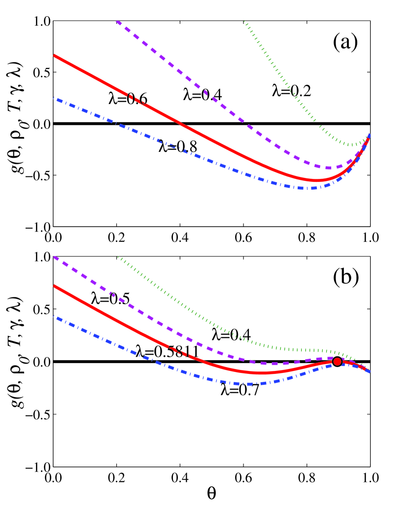
Figure 2: (Color online) Illustration of graphical solutions of Eq. (15). For ER random networks, (a) continuously increasing behavior of $R(\infty)$ with $\lambda$ for $T=1$, (b) discontinuous change in $R(\infty)$ for $T=3$. The black solid lines are the horizontal axis and the red dots denote the tangent points. Other parameters are $\rho_{0}=0.1$ and $\gamma=1.0$.

Now suppose that $\rho_{0}$ is not vanishingly small so that $\theta(\infty)=1$ is no longer a solution of Eq. (15). In this case, regardless of the values of other parameters, a finite fraction of individuals will adopt the behavior. It is thus reasonable to focus on how non-redundant information memory characteristic affects the dependence of the final behavioral adoption size $R(\infty)$ on the transmission probability $\lambda$, which can be obtained from the roots of Eq. (15). We are particularly interested in finding out whether the dependence is continuous or discontinuous. Note that the number of roots Eq. (15) is odd (including multiplicity) for any parameters, because of the $g[\theta(\infty),\rho_{0},T,\gamma,\lambda]<0$ for $\theta(\infty)=1$ and $g[\theta(\infty),\rho_{0},T,\gamma,\lambda]>0$ for $\theta(\infty)=0$. As shown in Figs. 2(a) and 2(b), numerical calculations indicate that the number of roots is either 1 or 3. When we fix all the parameters except $\lambda$, if Eq. (15) has only one root for different values of $\lambda$ [Fig. 2(a)], $R(\infty)$ will increase continuously with $\lambda$. If the number of roots of Eq. (15) depends on $\lambda$, as shown in Fig. 2(b), there will be three roots (fixed points), which means a saddle-node bifurcation occurs Strogatz2005 . The bifurcation analysis of Eq. (15) reveals that the system undergoes a cusp catastrophe: Varying $\lambda$, one finds that the physically meaningful stable solution of $\theta(\infty)$ will suddenly jump to an alternate outcome. In this case, a discontinuous growth pattern of $R(\infty)$ with $\lambda$ emerges, and the critical transmission probability $\lambda_{c}^{I}$ at which the discontinuity occurs can be obtained by solving Eqs. (15) and (17)-(18).

The discontinuous behavior in $R(\infty)$ versus $\lambda$ can be understood by using a specific example, e.g., by setting $T=3$. As shown in Fig. 2(b), for different values of $\lambda$, the function $g[\theta(\infty),\rho_{0},T,\gamma,\lambda]$ is tangent to horizontal axis at $\lambda_{c}^{I}\approx 0.5811$. For $\lambda<\lambda_{c}^{I}$, if Eq. (15) has 3 fixed points then the solution will be given by the largest one (since only this value can be achieved physically). Otherwise, the solution is the only fixed point. For $\lambda=\lambda_{c}^{I}$, the solution is given by the tangent point. For $\lambda>\lambda_{c}^{I}$, the only fixed point is the solution of Eq. (15). In this case, the solution of Eq. (15) changes abruptly to a small value from a relatively large value at $\lambda=\lambda_{c}^{I}$, leading to a discontinuous change in $R(\infty)$.

Finally, to determine the critical system parameter value of $\theta_{s}(\infty)$, across which the dependence of $R(\infty)$ on $\lambda$ changes from being continuous (discontinuous) to discontinuous (continuous), we can numerically solve Eqs. (15) and (16) together with the condition

$$\frac{d^{2}g[\theta(\infty),\rho_{0},T,\gamma,\lambda]}{d\theta^{2}(\infty)}=0.$$ (25)

From Eq. (25), we obtain

$$\rho_{0}^{s}=\frac{1}{\digamma},$$ (26)

where $\digamma=\sum_{k^{\prime}}k^{\prime}P(k^{\prime})\frac{d\Theta^{2}(k^{\prime},\theta(\infty))}{d\theta^{2}(\infty)}$. Using Eqs. (6) and (21), we get

$$\begin{split}\frac{d\Theta^{2}(k^{\prime},\theta(\infty))}{d\theta^{2}(\infty)}&=\sum_{m=0}^{T_{k^{\prime}}-1}\binom{k^{\prime}-1}{m}\\ &\times\{(k^{\prime}-m-1)[(k^{\prime}-m-2)\theta(\infty)^{k^{\prime}-m-3}\\ &\times(1-\theta(\infty))^{m}-m\theta(\infty)^{k^{\prime}-m-2}(1-\theta(\infty))^{m-1}]\\ &-m[(k^{\prime}-m-1)\theta(\infty)^{k^{\prime}-m-2}(1-\theta(\infty))^{m-1}\\ &-(m-1)\theta(\infty)^{k^{\prime}-m-1}(1-\theta(\infty))^{m-2}]\}.\end{split}$$ (27)

Combining Eqs. (15), (16) and (25), we get the value of $\theta_{s}(\infty)$. For fixed $T$ and $P(k)$, the critical values of other system parameters e.g., $\lambda_{c}^{s}$ and $\rho_{0}^{s}$, can then be determined.

IV Numerical verification

We perform extensive simulations on the spreading threshold model. In our simulations, we use Erdős-Rényi (ER) network model Erdos1959 and configuration network model with power-law degree distribution Catanzaro2005 , where the network size and mean degree are $N=10^{4}$ and $\langle k\rangle=10$, respectively. At least $2\times 10^{3}$ independent dynamical realizations on a fixed network are used to calculate the pertinent average values, which are further averaged over $100$ network realizations. We separately discuss the effects of dynamical and topological parameters.

IV.1 Effects of dynamical parameters

To be illustrative, we use ER random networks Erdos1959 . We first calculate the time evolution of the population densities for $\lambda=0.8$, $\rho_{0}=0.1$, $T=3$, and $\gamma=0.5$, as shown in Fig. 3(a), where we observe that the density of the susceptible (recovered) individuals decreases (increases) with time, and reaches some final value for large time. The density of the adopted individuals decreases initially (due to the fact that the number of individuals who newly adopt the behavior is less than that of individuals who become recovered), then increases and reaches a maximum value at $t\approx 5$. These results agree well with the predictions from our edge-based compartmental theory [see lines in Fig. 3(a)].

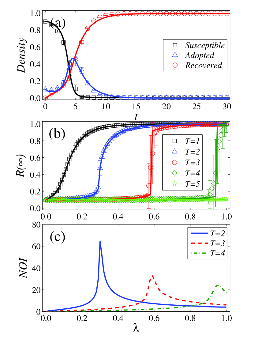
Figure 3: (Color online) Spreading threshold model on ER networks. (a) Average densities of susceptible, adopted, and recovered populations, denoted by $S(t)$ (black squares), $A(t)$ (blue up triangles), and $R(t)$ (red circles), respectively, versus time. (b) Final behavior adoption size $R(\infty)$ versus the transmission probability $\lambda$ for $T=1$ (black squares), $T=2$ (blue up triangles), $T=3$ (red circles), $T=4$ (dark green diamonds), and $T=5$ (light green stars) in the steady state. (c) Simulation results of NOI (number of iterations) as a function of $\lambda$ with $T=2$ (blue solid line), $T=3$ (red dashed line) and $T=4$ (dark dash dotted green line). The error bars indicate the standard deviations. The lines in (a) and (b) are theoretical predictions based on solutions of Eqs. (1)-(3) and (12)-(14). In (a), we set $\lambda=0.8$, $\rho_{0}=0.1$, $T=3$, and $\gamma=0.5$ (so as to obtain longer evolution time), while in (b) and (c), we set $\rho_{0}=0.1$ and $\gamma=1.0$.

We next study the final behavior adoption size $R(\infty)$ as a function of the transmission probability $\lambda$ for different values of the adoption threshold $T$ at another value of $\gamma=1.0$. As shown in Fig. 3(b), increasing $T$ impedes individuals from adopting the behavior, since a larger value of $T$ requires the individual to be exposed with more information from distinct neighbors to affirm the authority and legality of the behavior. As a result, individuals hardly adopt the behavior when the adoption threshold is relatively large (e.g., $T\geq 5$). Lines from the theory in Fig. 3(b) are very consistent with these simulation results. Through the bifurcation analysis of Eq. (15), we note that the adoption threshold affects strongly the manner by which $R(\infty)$ increases with $\lambda$ for $T\leq 4$. As shown in Fig. 3(b), for some small adoption threshold (e.g., $T=1$), $R(\infty)$ increases continuously with $\lambda$. However, for a slightly larger adoption threshold (i.e., $T\gtrsim 1$), the $R(\infty)$ versus $\lambda$ pattern becomes discontinuous, exhibiting an abrupt increase at some critical value $\lambda_{c}^{I}$. The statistical errors are generally small except for $\lambda$ close to $\lambda_{c}^{I}$ (for this reason and for figure clarity the error bars will not be shown for subsequent figures). The theoretical value of $\lambda_{c}^{I}$ can be calculated from Eqs. (15) and (17)-(18). The critical value can also be estimated by observing the number of iterations Parshani2011 ; Liu2012 (denoted as NOI, where only those iterations at which at least one individual adopts the behavior are taken into account). We observe that the NOI exhibits a maximum value at $\lambda_{c}^{I}$, e.g., for $T=2$, $3$, and $4$, as shown in Fig. 3(c). Overall, there is a remarkable agreement between theory and numerics in terms of the quantities $R(\infty)$ and $\lambda_{c}^{I}$. Through extensive simulations and theoretical predictions, we know the abandon probability doesn’t qualitatively affect the growth patterns of $R(\infty)$, so it is set as $\gamma=1.0$ in the rest of this paper.

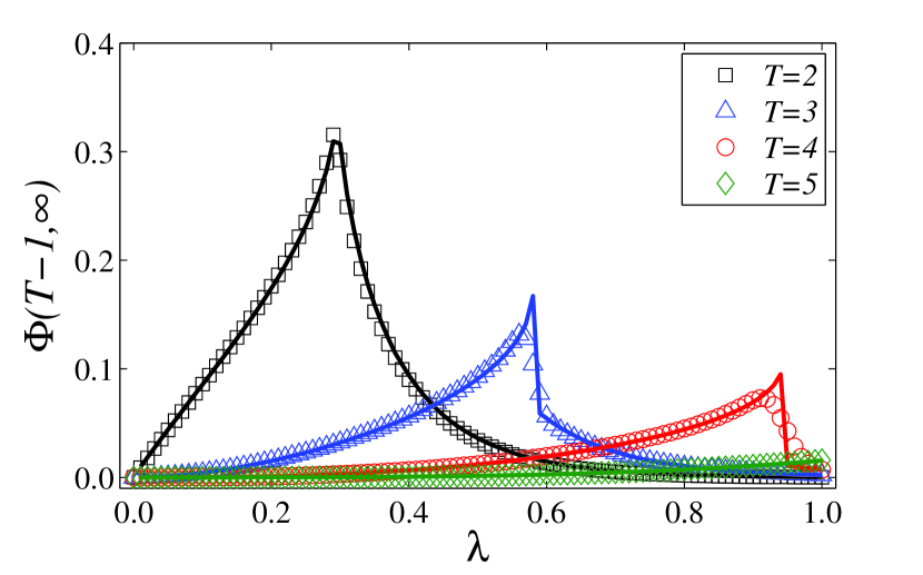
Figure 4: (Color online) The final fraction of individuals in the subcritical state on ER networks. $\Phi(T-1,\infty)$ versus $\lambda$ for $T=2$ (black squares), $T=3$ (blue up triangles), $T=4$ (red circles) and $T=5$ (dark green diamonds). The lines are theoretical predictions based on solutions of Eqs. (1), (4) and (12)-(14). Other parameters are $\gamma=1.0$ and $\rho_{0}=0.1$.

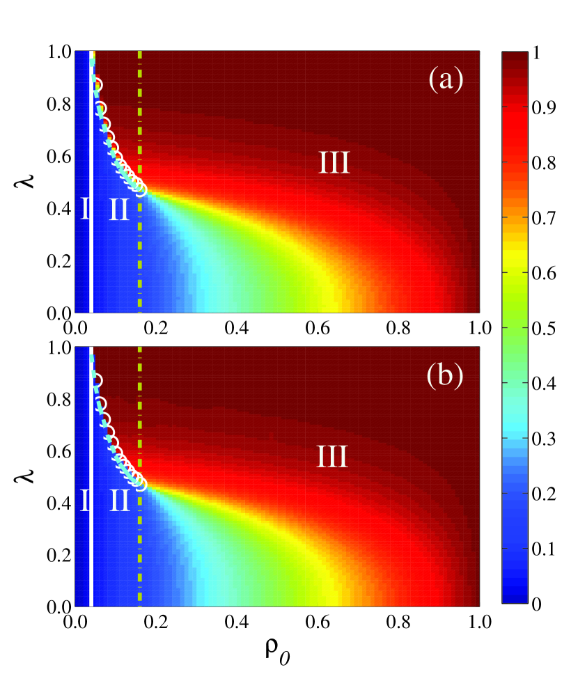
Figure 5: (Color online) Dependence of final behavior adoption size on initial seed size and transmission probability. For spreading threshold model on ER random networks, color-coded values of $R(\infty)$ from numerical simulations (a) and theoretical solutions (b) in the parameter plane ($\rho_{0}$,$\lambda$), where the theoretical values are from solutions of Eqs. (1)-(3) and (12)-(14). The numerically obtained critical values of the transmission probability, $\lambda_{c}^{I}$ (white circles), are from the NOI method, and the corresponding theoretical values blue dashed line) are from Eqs. (15) and (17)-(18). In each subfigure, three regions are shown: only a vanishingly small fraction of individuals can be exposed to adopt the behavior in region I, in region II $R(\infty)$ grows discontinuously with $\lambda$ and a finite fraction of individuals adopt the behavior above $\lambda_{c}^{I}$, and $R(\infty)$ grows continuously to a large value in region III. The vertical white solid lines and dash dotted yellow lines separate the plane into the three regions, which are predicted from our edge-based compartmental theory. Other parameters are $\gamma=1.0$ and $T=3$.

It is useful to identify the key factors that affect the dependence of $R(\infty)$ on $\lambda$. To obtain an intuitive understanding of the phenomenon of abrupt increase in $R(\infty)$ as $\lambda$ passes through a critical point, we focus on the individuals in the subcritical state. An individual $u$ in such a state has received the information but has not yet adopted the behavior, and the number of information pieces from distinct neighbors is precisely one less than the adoption threshold. Say at the time $u$ has received information from his/her neighbors except neighbor $v$. Now assume that $v$ has adopted the social behavior and transmits the information to $u$ successfully so as to cause $u$ to adopt the behavior. In turn, $u$ will transmit the information to his/her susceptible neighbors with probability $\lambda$, which will cause some subcritical state neighbors to adopt the behavior accordingly, and so on, potentially leading to an avalanche of behavior adoption. If the system has a relatively large number of individuals in the subcritical state, a slight increase in the number of individuals who adopt the behavior, e.g., by increasing the value of $\lambda$ slightly, may cause a sudden and large number of such subcritical state individuals with information pieces greater than their threshold, leading to a discontinuous “jump” in the value of $R(\infty)$. The above intuitive understanding is further proved by numerical simulations and theoretical predictions in Fig. 4. For $2\leq T<5$, the final fraction of individuals in subcritical state $\Phi(T-1,\infty)$ first increases with $\lambda$ below $\lambda_{c}^{I}$, $\Phi(T-1,\infty)$ reaches a maximum at the $\lambda_{c}^{I}$; and a slight increment of $\lambda$ induces a finite fraction of $\Phi(T-1,\infty)$ to adopt the behavior simultaneously, which leads to a discontinuous jump in the value of $R(\infty)$. When this social reinforcement effect is not present [e.g., $T=1$ in Fig. 3(b)], there are essentially no individuals in the subcritical state. In this case, $R(\infty)$ increases continuously with $\lambda$. We mention that the mechanism underlying the discontinuous increase in $R(\infty)$ in our spreading threshold model is similar to that responsible for phenomena such as explosive percolation Achlioptas2010 , bootstrap percolation Baxter2010 , k-core percolation Dorogovtsev2006 and explosive synchronization Gomez-Gardenes2011 .

We further investigate the role of the initial seed size $\rho_{0}$ in social contagion dynamics for relatively larger values of $T$, e.g., $T=3$. As shown in Fig. 5, we see that $R(\infty)$ increases with $\rho_{0}$, since individuals in the network have more chances to be exposed to the information. Based on the values of $R(\infty)$, we can divide the phase diagram into local ($\rho_{0}<0.04$) and global ($0.04\leq\rho_{0}\leq 1$) behavior adoption regions, where in the former (i.e., region I), only a vanishingly small fraction of individuals can be exposed to adopt the behavior and, in the latter including regions II and III, a finite fraction of individuals adopt the behavior and a crossover phenomenon occurs in the dependence of $R(\infty)$ on $\lambda$. The crossover phenomenon means that the dependence of $R(\infty)$ on $\lambda$ can change from being discontinuous to being continuous. More specifically, the saddle-node bifurcation of Eq. (15) occurs for $0.04\leq\rho_{0}\leq 0.15$ (region II in Fig. 5), thus $R(\infty)$ versus $\lambda$ is discontinuous; $R(\infty)$ versus $\lambda$ is continuous for $0.15<\rho_{0}\leq 1$ (region III in Fig. 5), as the saddle-node bifurcation disappears. The crossover phenomenon originates from the fact that the number of individuals in the subcritical state decreases with $\rho_{0}$. At the crossover or switching point $\rho_{0}^{s}$, as indicated by the vertical yellow dash dotted line in Fig. 5, the behavior of $R(\infty)$ versus $\lambda$ changes from being discontinuous to continuous. The crossover point can be calculated analytically by solving Eqs. (15)-(16) and (25). We also find that $\lambda_{c}^{I}$ decreases with $\rho_{0}$, since a large value of $\rho_{0}$ enhances the probability of individuals’ exposure to the information. In short, $R(\infty)$ versus the parameter plane $(\rho_{0},\lambda)$ shows a cusp catastrophe (i.e., the crossover phenomenon) Strogatz2005 . Regardless of the size of the initial seeds, there is a good agreement between numerically calculated and theoretically predicted behaviors of $R(\infty)$.

IV.2 Effects of topological parameters

We turn to elucidating the effect of network topological parameters on social contagion dynamics in our spreading threshold model. In fact, both the value of $R(\infty)$ and its pattern depend strongly on the mean degree and degree heterogeneity of the network. To be concrete, we first examine ER random networks with different values of the mean degree $\langle k\rangle$, as shown in Fig. 6, where we see that $R(\infty)$ increases with $\langle k\rangle$ in general, since individuals with larger degrees have higher probabilities to be exposed to information from distinct neighbors, leading to a high likelihood that they adopt the behavior as well. By the bifurcation analysis of Eq. (15), we find that with the increase of $\langle k\rangle$, the growth pattern of $R(\infty)$ changes from being continuous to being discontinuous. For a small value of the mean degree (e.g., $\langle k\rangle=5$), only a small fraction of the individuals adopt the behavior, so $R(\infty)$ changes with $\lambda$ continuously. For a relatively larger value of the mean degree (e.g., $\langle k\rangle>5$), more individuals adopt the behavior, leading to a sudden, discontinuous increase in $R(\infty)$ with $\lambda$. As discussed in Sec. IV.1, the “explosive” growth of $R(\infty)$ occurs whenever there is a finite but sizable fraction of individuals in the subcritical state, which cannot happen when the mean degree of the network is small. We also observe that increasing the mean degree can reduce the value of the critical point $\lambda_{c}^{I}$, due to the corresponding increase in the number of individuals having relatively large degrees.

We next study scale-free networks. Figure 7 shows, for $T=3$, $R(\infty)$ versus $\lambda$ for $\langle k\rangle=10$. The uncorrelated networks are generated with the power-law degree distribution $P(k)\sim k^{-\nu}$ ($\nu$ being the degree exponent) according to the procedure in Ref. Catanzaro2005 , where the maximum degree is set as $k_{max}\sim\sqrt{N}$. We find that increasing the heterogeneity of network structure (by using smaller values of the degree exponent) promotes (suppresses) $R(\infty)$ for small (large) values of $\lambda$. This result can be qualitatively explained as follows Wang2014A : From Eqs. (1)-(2), we know that hubs adopt the behavior with large probability. With the increase of network heterogeneity (i.e., decreasing $\nu$), the network has a large number of individuals with very small degrees and more individuals with large degrees. For small values of $\lambda$, more hubs for small $\nu$ facilitate behavior spreading as they are more likely to adopt the behavior. But for large values of $\lambda$, a large number of individuals with very small degrees have a small probability to adopt the behavior, resulting in smaller values of $R(\infty)$. By the bifurcation analysis of Eq. (15), we also observe that the system has a critical degree exponent $\nu^{s}\approx 4.0$, below which $R(\infty)$ versus $\lambda$ is continuous but above which the variation is discontinuous. That is, as the network becomes more heterogeneous, we expect a change in the dependence of $R(\infty)$ on $\lambda$ from being discontinuous to continuous, since the existence of strong degree heterogeneity can not make individuals in the subcritical state adopt the behavior simultaneously. We also note that the critical point $\lambda_{c}^{I}$ decreases as the network becomes more heterogeneous. Again, there is a good agreement between theoretical and numerical results.

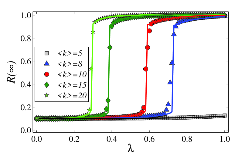
Figure 6: (Color online) Effect of mean network degree on social contagion dynamics. For ER random networks, $R(\infty)$ versus the transmission probability $\lambda$ for mean degree $\langle k\rangle=5$ (gray squares), $\langle k\rangle=8$ (blue up triangles), $\langle k\rangle=10$ (red circles), $\langle k\rangle=15$ (dark green diamonds), and $\langle k\rangle=20$ (light green stars). Other parameters are $\rho_{0}=0.1$, $\gamma=1.0$ and $T=3$. The lines are theoretical values of $R(\infty)$ calculated from Eqs. (1)-(3) and (12)-(14).

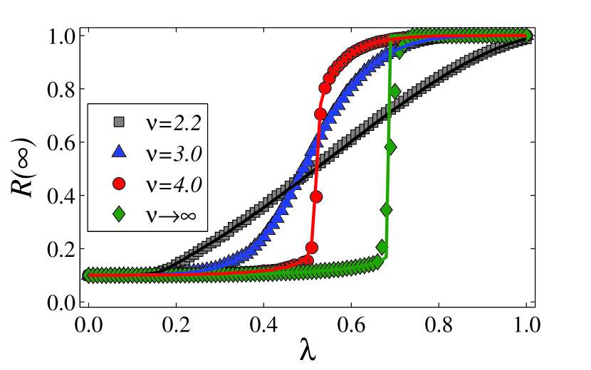
Figure 7: (Color online) Effect of network heterogeneity on social contagion dynamics. For scale-free networks, $R(\infty)$ versus $\lambda$ for degree exponent $\nu=2.2$ (gray squares), $\nu=3.0$ (blue up triangles), $\nu=4.0$ (red circles) and $\nu\rightarrow\infty$ (dark green diamonds). The case for $\nu\rightarrow\infty$ reduces to a random regular network with identical degree. The lines are theoretical values of $R(\infty)$ calculated from Eqs. (1)-(3) and (12)-(14). Other parameters are $\rho_{0}=0.1$, $\gamma=1.0$ and $T=3$.

V Alternative models of social contagion dynamics

The edge-based compartmental theory developed in Sec.III can be applied to more general social contagion dynamics with reinforcement effect derived from non-redundant information memory characteristic. Here, we demonstrate the use of our theory in analyzing two alternative, somewhat more complicated social contagion models: (1) correlated spreading threshold model in which the adoption threshold of each individual is correlated with his/her degree and (2) a generalized social contagion model in which the behavior adoption probability $\pi(k,m)$ is a monotonically increasing function of $m$.

V.1 Correlated spreading threshold model

In reality, whether an individual adopts certain social behavior depends on his/her personal characters such as age and habit, which are reflected by the corresponding degree in the social network. As a result, there is typically some correlation between an individual’s degree and his/her ability to adopt new social behaviors triggered by crossing the adoption threshold. For simplicity, we use a recently introduced relation Cui2014 to account for the correlation between individual $i$’s adoption threshold and degree $k_{i}$, as

$$T_{i}=A_{\alpha}(\frac{k_{i}}{k_{max}})^{\alpha},$$ (28)

where $k_{max}$ is the maximum degree, $A_{\alpha}$ and $\alpha$ are two adjustable parameters. For $\alpha=0$, the adoption threshold is uncorrelated with the degree, and all individuals in the network share the same adoption threshold. For $\alpha>0$, the adoption threshold is positively correlated with the degree, i.e., individuals with larger degrees have higher adoption thresholds, and the opposite occurs for $\alpha<0$.

To investigate the effects of varying $\alpha$ on social contagion dynamics using the spreading threshold model, we set the mean adoption threshold (somewhat arbitrarily) to be $\langle T\rangle=3$. The sum of the adoption threshold in the network is $T_{s}=\sum_{i=1}^{N}T_{i}$. For $\alpha=0$, we have $T_{s}=\langle T\rangle N=A_{\alpha=0}N$. Further, we get

$$A_{\alpha}=\frac{A_{\alpha=0}Nk_{max}^{\alpha}}{\sum_{i=1}^{N}k_{i}^{\alpha}}.$$ (29)

Evidence in terms of the quantity $R(\infty)$, which supports our edge-based compartmental theory for varying threshold as given by Eq. (28), is presented in Fig. 8. We observe a reasonable agreement between the theoretical predictions and simulation results. Note that $\alpha$ affects not only the value of $R(\infty)$ but also its dependence on $\lambda$. In particular, for $\alpha>0$, increasing $\alpha$ causes the critical point $\lambda_{c}^{I}$ first to increase then to decrease. This result can be qualitatively explained by noting that, slightly larger values of $\alpha$ (e.g, $\alpha=1$) can cause the individuals whose degrees are near the mean degree of the network to hold larger adoption threshold. However, much larger values of $\alpha$ (e.g., $\alpha=2$) will generate hubs with larger adoption threshold, thereby reducing the adoption threshold for the individuals with degrees near the mean degree. Since, in a random network, the degrees of most individuals are close to the mean degree, this causes the non-monotonic change in $\lambda_{c}^{I}$.

For $\alpha<0$, decreasing $\alpha$ facilitates individuals’ adopting the behavior, and the dependence of $R(\infty)$ on $\lambda$ changes from being discontinuous to continuous by the bifurcation analysis of Eq. (15). Decreasing $\alpha$ makes individuals with small (large) degrees to hold larger (smaller) adoption thresholds than the case of $\alpha=0$. As a result, the values of $R(\infty)$ are smaller than those for $\alpha=0$ in the large $\lambda$ regime. Since individuals with small degrees have relatively large adoption threshold, they have more difficulty in adopting the social behavior, further decreasing the number of individuals in the subcritical state and making the discontinuous behavior in $R(\infty)$ to disappear.

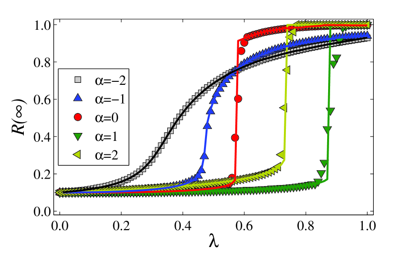
Figure 8: (Color online) Effect of degree-correlated spreading threshold on social contagion dynamics. For ER random networks, final adoption size $R(\infty)$ versus the transmission probability $\lambda$ for $\alpha=-2$ (gray squares), $\alpha=-1$ (blue up triangles), $\alpha=0$ (red circles), $\alpha=1$ (dark green diamonds), and $\alpha=2$ (yellow left triangles). Other parameters are $\langle k\rangle=10$, $\langle T\rangle=3$, and $\gamma=1.0$. The lines are theoretical values of $R(\infty)$ from solutions of Eqs. (1)-(3) and (12)-(14) with adoption threshold given by Eq. (29).

V.2 A generalized social contagion model

Recently, Centola performed an interesting experiment of the health behavior spreading in an online social network, and found that the behavior adoption probability is a monotonically increasing function of $m$ Centola2010 , but not the trivial case of Heaviside step function in the spreading threshold model and Refs. Dodds2004 ; Dodds2005 . Therefore, we assume that a susceptible individual adopts the behavior with probability

$$\pi(k,m)=1-(1-\epsilon)^{m},$$ (30)

where $m$ is the accumulated times that the individual has been exposed to different sources, i.e., he/she has received the information $m$ times from the distinct neighbors, and $\epsilon$ is the unit adoption probability. We can also use the edge-based compartmental theory to analyze the dynamical process of this model by substituting Eq. (30) into various equations that give the solutions of e.g., $R(\infty)$. In particular, we rewrite Eqs. (2) and (7) as

$$s(k,t)=\sum_{m=0}^{k}\phi_{m}(k,t)(1-\epsilon)^{\sum_{j=1}^{m}j}$$ (31)

and

$$\Theta(k^{\prime},\theta(t))=\sum_{m=0}^{k^{\prime}-1}\tau_{m}(k^{\prime},\theta(t))(1-\epsilon)^{\sum_{j=0}^{m}j},$$ (32)

respectively, whereas Eq. (13) has the same form as Eq. (22). The different aspect is that we need to replace Eq. (23) with

$$\begin{split}\psi(t)&=(1-\rho_{0})\sum_{k=0}^{\infty}P(k)\sum_{m=0}^{k}\binom{k}{m}(1-\epsilon)^{\sum_{i=0}^{m}i}\\ &\times[(k-m)\theta(t)^{k-m-1}[1-\theta(t)]^{m}\\ &-m\theta(t)^{k-m}[1-\theta(t)]^{m-1}].\end{split}$$ (33)

Substituting Eqs. (31)-(33) into the corresponding equations, we can obtain a theoretical understanding of the dynamical evolution of the generalized social contagion model. We observe that $R(\infty)$ varies with $\lambda$ continuously by the bifurcation analysis of Eq. (15). The theoretical values of $R(\infty)$ so predicted agree well with the simulated results, as shown in Fig. 9.

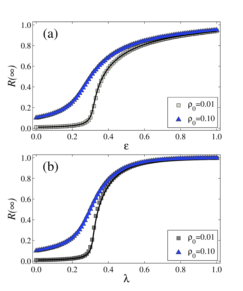
Figure 9: (Color online) Results from a generalized social contagion model. For ER networks, $R(\infty)$ versus the unit adoption probability $\epsilon$ for $\lambda=0.3$ (a) and the transmission probability $\lambda$ for $\epsilon=0.3$ (b). Two values of $\rho_{0}$ are used: $\rho_{0}=0.01$ (gray squares) and $\rho_{0}=0.10$ (blue up triangles). Additional parameters are $\gamma=1.0$ and $\langle k\rangle=10$. In both panels, the lines represent the theoretical values of $R(\infty)$ obtained from solutions of Eqs. (1)-(3) and (12)-(14) with $\psi(t)$ given by (33).

VI Conclusions

In social contagion dynamics, memory of non-redundant information can have a significant impact on the reinforcement mechanism required for behavioral adoption. In particular, the non-redundant information memory has two features: (1) repetitive information transmission on every edge is forbidden, (2) every individual can remember the cumulative pieces of non-redundant information. Social reinforcement incorporating the memory characteristic is essential to describing and understanding social contagions in the real world. In this paper, we first proposed a general social contagion model with reinforcement derived from this memory characteristic. Mathematically, a model based on such characteristic is necessarily non-Markovian. Previous works pointed out the difficulty to develop an accurate theoretical framework to analyze social contagion dynamics with only memory effect Dodds2004 , let alone models with non-redundant information memory characteristic. To meet this challenge, in this paper we developed a unified edge-based compartmental theory to analyze social contagion dynamics with non-redundant information memory characteristic. The validity of our theory is established by testing it using different social contagion models of varying complexity, different model networks.

Through a detailed study of a comparatively simple model, the spreading threshold model, the effects of non-redundant information memory characteristic on the social contagion dynamics can be quantified by the final adoption size $R(\infty)$ and its dependence on key parameters such as $\lambda$. Especially, decreasing the adoption threshold, increasing the initial seed size or increasing the mean degree of the network can facilitate adoption of social behaviors at the individual level, making the system less resilient to social contagions. The effect of structural heterogeneity on $R(\infty)$ turns out to be more complex in that, while making the network more heterogeneous can promote the spreading process, it impedes spreading for relatively large values of $\lambda$. A striking phenomenon is that $R(\infty)$ as a function of $\lambda$ can exhibit two characteristically different types of patterns: continuous variation or sudden, discontinuous changes, and a transition between the two patterns can be induced by adjusting parameters such as individuals’ adoption threshold, the initial seed size or the structural heterogeneity of the network. For example, in order to change the dependence of $R(\infty)$ on $\lambda$ from being discontinuous to continuous, we can decrease the individuals’ adoption threshold, increase the initial seed size or make the network more heterogeneous. We also find that the discontinuous pattern disappears when there is negative correlation between individual’s adoption threshold and his/her degree. The above crossover phenomena can be understood through the bifurcation analysis in theory, and also justified by analyzing the subcritical individuals in simulations.

To study social contagion dynamics in human populations is an extremely challenging problem with broad implications and interest. Our main contribution is a treatment of the non-redundant information memory characteristic that is intrinsic to real world dynamics of social contagions. Our unified edge-based compartmental theory gives reasonable understanding of the roles of the memory characteristic in shaping the spreading dynamics, which can be applied to analyzing different dynamical processes such as information diffusion on computer networks. However, many challenges remain, such as incorporation of correlations between local structures (e.g., communities and motifs) into social reinforcement effect at the individual level, the impacts of redundant versus non-redundant information transmission, and further development of analytic methods to treat non-Markovian social contagion model on more realistic networks such as clustered Serrano2006 ; Newman2009 , multiplex Boccaletti2014 ; Wang2014B ; Salehi2014 ; Kivela2014 ; Lee2015 , and temporal networks Holme2012 ; Barrat2013 ).

- (1) C. Castellano, S. Fortunato, and S. Fortunato, Rev. Mod. Phys. 81, 0034 (2009).
- (2) H. P. Young, Proc. Natl Acad. Sci. USA 108, 21285 (2011).
- (3) D. Centola, Science 334, 1269 (2011).
- (4) A. Banerjee, A. G. Chandrasekhar, E. Duflo, and M. O. Jackson, Science 341, 363 (2013).
- (5) D. Centola, Science, 329, 1194 (2010).
- (6) P. S. Dodds and D. J. Watts, Phys. Rev. Lett. 92, 218701 (2004).
- (7) P. S. Dodds and D. J. Watts, J Thor. Biol. 232, 587 (2005).
- (8) C. H. Weiss, J. Poncela-Casasnovas, J. I. Glaser, A. R. Pah, S. D. Persell, D. W. Baker, R. G. Wunderink, and L. A. NunesAmaral, Phys. Rev. X 4, 041008 (2014)
- (9) D. Centola and M. Macy, Am. J. Sociol. 113, 702 (2007).
- (10) M. Granovetter, Am. J. Sociol. 78, 1360 (1973).
- (11) D. J. Watts, Proc. Natl. Acad. Sci. USA 99, 5766 (2002).
- (12) M. E. J. Newman, Phys. Rev. E 66, 016128 (2002).
- (13) R. Pastor-Satorras and A. Vespignani, Phys. Rev. Lett. 86, 3200 (2001).
- (14) M. Boguñá, C. Castellano, and R. Pastor-Satorras, Phys. Rev. Lett. 111, 068701 (2013).
- (15) C. Castellano and R. Pastor-Satorras, Phys. Rev. Lett. 105, 218701 (2010).
- (16) J. P. Gleeson and D. J. Cahalane, Phys. Rev. E 75, 056103 (2007).
- (17) D. E. Whitney, Phys. Rev. E 82, 066110 (2010).
- (18) J. P. Gleeson, Phys. Rev. E 77, 046117 (2008).
- (19) A. Nematzadeh, E. Ferrara, A. Flammini, and Y.-Y. Ahn, Phys. Rev. Lett. 113, 088701 (2014).
- (20) K.-M. Lee, C. D. Brummitt, and K.-I. Goh, Phys. Rev. E 90, 062816 (2014).
- (21) C. D. Brummitt, K.-M. Lee, and K.-I. Goh, Phys. Rev. E 85, 045102(R) (2012).
- (22) O. Yaǧan and V. Gligor, Phys. Rev. E 86, 036103 (2012).
- (23) T. Takaguchi, N. Masuda, and P. Holme, PLoS ONE 8, e68629 (2013).
- (24) F. Karimi and P. Holme, Physica A 392, 3476 (2013).
- (25) K. Chung, Y. Baek, D. Kim, M. Ha, and H. Jeong, Phys. Rev. E 89, 052811 (2014).
- (26) S. Aral and D. Walker, Science 337, 337 (2012).
- (27) L. Lü, D.-B. Chen, and T. Zhou, New. J. Phys. 13, 123005 (2011).
- (28) J. Ugander, L. Backstrom, C. Marlow, and J. Kleinberg, Proc. Natl. Acad. Sci. USA 109, 5962 (2012).
- (29) P. V. Mieghem and R. van de Bovenkamp, Phys. Rev. Lett. 110, 108701 (2013).
- (30) E. Cator, R. van de Bovenkamp, and P. V. Mieghem, Phys. Rev. E 87, 062816 (2013).
- (31) R. Pastor-Satorras, C. Castellano, P. V. Mieghem, and A. Vespignani, arXiv:1408.2701v1 (2014).
- (32) M. Catanzaro, M. Boguñá, and R. Pastor-Satorras, Phys. Rev. E 71, 027103 (2005).
- (33) F. J. Pérez-Reche, J. J. Ludlam, S. N. Taraskin, and C. A. Gilligan, Phys. Rev. Lett. 106, 218701 (2011).
- (34) M. Karsai, G. In̋iguez, K. Kaski, and J. Kertész, J. R. Soc. Interface 11, 101 (2014).
- (35) P. S. Dodds, K. D. Harris, and C. M. Danforth, Phys. Rev. Lett. 110, 158701 (2013).
- (36) K. D. Harris, C. M. Danforth, and P. S. Dodds. Phys. Rev. E 88, 022816 (2013).
- (37) G. J. Baxter, S. N. Dorogovtsev, A. V. Goltsev, and J. F. F. Mendes, Phys. Rev. E 82, 011103 (2010).
- (38) Y. C. Zhang, Phys. Rev. Lett. 63, 470 (1989).
- (39) J. C. Miller, A. C. Slim, and E. M. Volz, J. R. Soc. Interface. 10, 1098 (2011).
- (40) J. C. Miller and E. M. Volz, PLoS ONE, 8(8), e69162 (2013).
- (41) L. D. Valdez, P. A. Macri, and L. A. Braunstein, PLoS ONE, 7: e44188 (2014).
- (42) W. Wang, M. Tang, H.-F. Zhang, H. Gao, Y. Do, and Z.-H. Liu, Phys. Rev. E 90, 042803 (2014).
- (43) B. Karrer and M. E. J. Newman, Phys. Rev. E 82, 016101 (2010).
- (44) S. H. Strogatz, Nonlinear dynamics and chaos: with applications to physics, biology, chemistry and engineering (Westview, Boulder, CO, 1994).
- (45) P. Erdős and Rényi, Publ. Math. 6, 290 (1959).
- (46) R. Parshani, S. V. Buldyrev, and S. Havlin, Proc. Natl. Acad. Sci. USA 108, 1007 (2011).
- (47) R.-R. Liu, W.-X. Wang, Y.-C. Lai, and B.-H. Wang, Phys. Rev. E 85, 026110 (2012).
- (48) D. Achlioptas, R. M. D Souza, and J. Spencer, Science, 323, 1453 (2009).
- (49) S. N. Dorogovtsev, A. V. Goltsev, and J. F. F. Mendes, Phys. Rev. Lett. 96, 040601 (2006).
- (50) J. Gómez-Gardeñes, S. Gómez, A. Arenas, and Y. Moreno, Phys. Rev. Lett. 106, 128701 (2011).
- (51) A.-X. Cui, W. Wang, M. Tang, Y. Fu, X. Liang, Chaos 24, 033113 (2014).
- (52) M. Á. Serrano and M. Boguñá, Phys. Rev. Lett. 97, 088701 (2006).
- (53) M. E. J. Newman, Phys. Rev. Lett. 103, 058701 (2009).
- (54) S. Boccaletti, G. Bianconi, R. Criado, C. I. del Genio, J. Gómez-Gardeñes, M. Romance, I. Sendiña-Nadal, Z. Wang, and M. Zanin, Phys. Rep. 10, 1016 (2014).
- (55) W. Wang, M. Tang, H. Yang, Y. Do, Y.-C. Lai, and G.W. Lee, Sci. Rep. 4, 5097 (2014).
- (56) M. Salehi, R. Sharma, M. Marzolla, M. Magnani, P. Siyari, and D. Montesi, arXiv:1405.4329 (2014).
- (57) K.-M. Lee, B. Mina, and K.-I. Goh, Eur. Phys. J. B 88, 48 (2015).
- (58) M. Kivelä, A. Arenas, M. Barthelemy, J. P. Gleeson, Y. Moreno, and M. A. Porter, J. Complex Netw. 2, 203 (2014).
- (59) P. Holme and J. Saramäki, Phys. Rep. 519, 97 (2012).
- (60) A. Barrat, B. Fernandez, K. K. Lin, and L.-S. Young, Phys. Rev. Lett. 110, 158702 (2013).