Optimizing the geometrical accuracy of curvilinear meshes

Abstract

This paper presents a method to generate valid high order meshes with optimized geometrical accuracy. The high order meshing procedure starts with a linear mesh, that is subsequently curved without taking care of the validity of the high order elements. An optimization procedure is then used to both untangle invalid elements and optimize the geometrical accuracy of the mesh. Standard measures of the distance between curves are considered to evaluate the geometrical accuracy in planar two-dimensional meshes, but they prove computationally too costly for optimization purposes. A fast estimate of the geometrical accuracy, based on Taylor expansions of the curves, is introduced. An unconstrained optimization procedure based on this estimate is shown to yield significant improvements in the geometrical accuracy of high order meshes, as measured by the standard Haudorff distance between the geometrical model and the mesh. Several examples illustrate the beneficial impact of this method on CFD solutions, with a particular role of the enhanced mesh boundary smoothness.

1 Introduction

The development of high-order numerical technologies for engineering analysis has been underway for many years now. For example, Discontinuous Galerkin methods (DGM) have been thoroughly studied in the literature, initially in a theoretical context [7], and now from the application point of view [14, 15]. Compared to standard second-order-accurate numerical schemes, high-order methods exhibit superior efficiency in problems with high resolution requirements, because they reach the required accuracy with much coarser grids.

However, many contributions have pointed out that the accuracy of these methods can be severely hampered by a too crude discretization of the geometry [4, 5, 22]. It is now widely accepted that linear geometrical discretizations may annihilate the benefits of high-order schemes in cases featuring curved geometries, that is, in most cases of engineering and scientific interest.

This problem has motivated the development of methods for the generation of high-order meshes, in which curvilinear elements are meant to provide sufficient geometrical accuracy on the boundary. Elements are then most often defined in a Lagrangian manner by a set of high-order nodes. Until now, efforts have mostly been targeted at ensuring the validity of the mesh. Indeed, the naive approach consisting in simply curving the boundaries of a linear mesh to match the geometry often results in tangled elements [24]. The curvature of the boundary must somehow be “propagated” into the domain for all elements to be valid. In the case of locally structured meshes, such a situation can be avoided by means of an efficient isoparametric technique [17]. For unstructured meshes, untangling procedures based on topological operations [8, 16, 20], mechanical analogies [26, 1, 18] or optimization procedures [10, 24] have been proposed.

Although the improved representation of the geometry of the domain is the prime motivation for the use of high-order meshes, only few authors have taken into consideration the quality of the geometrical approximation. In the literature, the limited work dedicated to this topic has focused on placing adequately the high-order nodes when curving the mesh boundaries. Simple techniques include interpolating them between the first-order boundary nodes in the parametric space describing the corresponding CAD entity [8, 10] or projecting them on the geometry from their location on the straight-sided element. More sophisticated procedures have also been proposed. In Ref. [26], the high-order nodes on boundary edges are interpolated in the physical space through a numerical procedure involving either the CAD parametrization (in the case of a mesh edge assigned to an edge of the geometric model), or an approximation of the geodesic connecting the two first-order vertices (in the case of an edge located on a 3D surface). Nodes located within surface elements are obtained through a more sophisticated version of this procedure. Instead of interpolating, Sherwin and Peiró [21] use a mechanical analogy with chains of springs in equilibrium that yields the adequate node distribution along geometric curves and geodesics for edge nodes. Two-dimensional nets of springs provide the appropriate distribution of surface element nodes.

This paper presents a method that makes it possible to build geometrically accurate curvilinear meshes. Unlike previous work reported in the literature, the representation of the model by the mesh is formally assessed by measuring distances between the geometric model and the corresponding high-order mesh boundary, or by evaluating a fast estimate of the geometrical error. The aim of the method is to minimize this geometrical error through the use of standard optimization algorithms. Although most of the paper deals with two-dimensional meshes, it is shown that the approach can easily be extended to three spatial dimensions.

Consider a model entity ${\mathcal{C}}$ and the mesh entity ${\mathcal{C}}_{m}$ that is meant to approximate ${\mathcal{C}}$. The first questions that arise are how to define a proper distance $d({\mathcal{C}},{\mathcal{C}}_{m})$ between ${\mathcal{C}}$ and ${\mathcal{C}}_{m}$, and how to compute this distance efficiently. Two main definitions for such a distance have been proposed in the computational geometry literature, namely the Fréchet distance and the Hausdorff distance.

In this context of curvilinear meshing, distances $d({\mathcal{C}},{\mathcal{C}}_{m})$ that are computed are usually small in comparison with the typical dimension of either ${\mathcal{C}}$ or ${\mathcal{C}}_{m}$. Consequently, $d({\mathcal{C}},{\mathcal{C}}_{m})$ has to be computed with high accuracy. In this paper, we show that computing standard distances between the mesh and the geometry may be too expensive for practical computations. Alternative measures of distance are presented, that are both fast enough to compute and sufficiently accurate. An optimization procedure is then developed to drastically reduce the model-to-mesh distance while enforcing the mesh validity.

The paper is organized as follows. In Section 2, the problem of defining and computing a proper model-to-mesh distance is examined. The mesh optimization procedure is described in Section 3. Section 4 illustrates the method with examples, and the extension of the approach to three dimensions is presented in Section 5. Conclusions are drawn in Section 6.

2 Model-to-Mesh Distance

2.1 Distance Between Curves

2.1.1 Setup

Consider the following planar parametric curve

$${\mathcal{C}}\equiv\{\eta\in[\eta_{0},\eta_{p}]\mapsto\text{\boldmath$x$\unboldmath}(\eta)\in R^{2}\}$$

and the following $p+1$ successive points on ${\mathcal{C}}$

$$\text{\boldmath$x$\unboldmath}_{i}=\text{\boldmath$x$\unboldmath}(\eta_{i}),~{}~{}\mbox{with}~{}~{}\eta_{0}<\eta_{1}<\eta_{2}\dots<\eta_{p-1}<\eta_{p}.$$

A curvilinear mesh edge ${\mathcal{C}}_{m}$ is defined as the Lagrange approximation of ${\mathcal{C}}$ at order $p$

$${\mathcal{C}}_{m}\equiv\left\{\xi\in[0,1]\mapsto\text{\boldmath$x$\unboldmath}_{m}(\xi)=\sum_{i=0}^{p}{\mathcal{L}}^{(p)}_{i}(\xi)\;\in R^{2}\right\}.$$ (1)

In (1), ${\mathcal{L}}^{(p)}_{i}(\xi)$ is the $i$th Lagrange polynomial of order $p$.

Curves ${\mathcal{C}}$ and ${\mathcal{C}}_{m}$ that are both bounded by the vertices $\text{\boldmath$x$\unboldmath}_{0}$ and $\text{\boldmath$x$\unboldmath}_{p}$ and coincide at least at the $p+1$ Lagrange points $\text{\boldmath$x$\unboldmath}_{i},~{}i=0,\dots,p$ (see Figure 1).

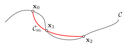
Figure 1: Typical setup: a model edge $\mathcal{C}$ and a quadratic mesh edge ${\mathcal{C}}_{m}$.

2.1.2 Formal Definitions of Distance

Define $\alpha(t)$ (resp. $\beta(t)$) as an arbitrary continuous nondecreasing function from $t\in[0,1]$ onto $\eta\in[\eta_{0},\eta_{p}]$ (resp. $\xi\in[0,1]$). The Fréchet distance between ${\mathcal{C}}$ and ${\mathcal{C}}_{m}$ is defined as

$$d_{\mathrm{F}}({\mathcal{C}},{\mathcal{C}}_{m})=\inf_{\alpha,\beta}\,\,\max_{t\in[0,1]}\|\text{\boldmath$x$\unboldmath}_{m}(\beta(t))-\text{\boldmath$x$\unboldmath}(\alpha(t))\|.$$

There is a standard interpretation of the Fréchet distance. Consider a man is walking with a dog on a leash. The man is walking on the one curve and the dog on the other one. Both may vary their speed, as $\alpha$ and $\beta$ are arbitrary. Backtracking is not allowed which implies that $\alpha$ and $\beta$ are non-decreasing. Then, the Fréchet distance between the curves is the minimal length of a leash that is necessary.

The Hausdorff distance between ${\mathcal{C}}$ and ${\mathcal{C}}_{m}$ is the smallest value $d$ such that every point of ${\mathcal{C}}$ has a point of ${\mathcal{C}}_{m}$ within distance $d$ and every point of ${\mathcal{C}}_{m}$ has a point of ${\mathcal{C}}$ within distance $d$ [19]. It is formally defined as

$$d_{\mathrm{H}}({\mathcal{C}},{\mathcal{C}}_{m})=\max\{\,\sup_{\eta\in[\eta_{0},\eta_{p}]}\inf_{\xi\in[0,1]}\|\text{\boldmath$x$\unboldmath}_{m}(\xi)-\text{\boldmath$x$\unboldmath}(\eta)\|,\,$$

$$\sup_{\xi\in[0,1]}\inf_{\eta\in[\eta_{0},\eta_{p}]}\|\text{\boldmath$x$\unboldmath}_{m}(\xi)-\text{\boldmath$x$\unboldmath}(\eta)\|\,\}\mbox{.}$$

Not only $d_{H}({\mathcal{C}},{\mathcal{C}}_{m})\leq d_{F}({\mathcal{C}},{\mathcal{C}}_{m})$, but the Fréchet distance between two curves can be arbitrarily larger than their Hausdorff distance. The Fréchet distance is usually considered as a more reliable measure of similarity between curves. Figure 2 shows two curves that can be made arbitrary “Hausdorff-close” while being quite dissimilar.

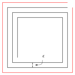
Figure 2: Two curves that can be made arbitrary close when $\epsilon\rightarrow 0$ in terms of their Hausdorff distance (that is exactly $3\epsilon$) but not in terms of their Fréchet distance that remains finite and equal to the diagonal of the square.

The definition of the Hausdorff and Fréchet measures, that involves infima and suprema over infinite sets of parametrizations, makes it difficult to devise algorithms for computing these distances between arbitrary curves. However, an alternative that can lead to practical algorithms is to calculate the Hausdorff and Fréchet distances between polygonal approximations of the curves under consideration, as explained in the next Section.

2.2 Distance Between Polygonal Curves

2.2.1 Optimal Sampling of Curves

Let us first consider the problem of approximating an arbitrary curve by a polygonal curve. In order to maximize the efficiency of the distance computation, it is necessary to find a polygonal curve that contains as few vertices as possible and still approximates the original curve with sufficient accuracy.

Assume $m+1$ points ${\bf{p}}_{i}=\text{\boldmath$x$\unboldmath}_{m}(\xi_{i}),~{}i\in[0,m],$ that are sampled on ${\mathcal{C}}_{m}$. This defines a polygonal curve $M$ formed of $m$ segments for which segment $i$ goes from ${\bf{p}}_{i}$ to ${\bf{p}}_{i+1}$ (see Fig. 3). Let us do the same with ${\mathcal{C}}$ and define a polygonal curve $N$ composed of $n+1$ points ${\bf{q}}_{i},~{}i\in[0,n].$

Figure 3: A model edge $\mathcal{C}$, a mesh edge ${\mathcal{C}}_{m}$ and a polygonal curve M (in blue).

The goal is to find sampling points on the original curve ${\mathcal{C}}_{m}$ (resp. $\mathcal{C}$) in such a way that the distance between the polygonal curve $M$ (resp. $N$) and ${\mathcal{C}}_{m}$ (resp. $\mathcal{C}$) is smaller than a threshold distance $\epsilon$.

A parametrization of ${\mathcal{C}}_{m}$ is given by (1) and a parametrization of $\mathcal{C}$ is usually available from the CAD model. A possible sampling strategy for these curves consists in starting with the segment $[\text{\boldmath$x$\unboldmath}_{0},\text{\boldmath$x$\unboldmath}_{p}]$ and refining recursively the discretization with points distributed uniformly in the parameter space, until the desired accuracy is reached. However, $\mathcal{C}$ is often a Bézier or a rational Bézier spline. As a polynomial curve, ${\mathcal{C}}_{m}$ is also a particular case of a Bézier curve. For such curves, de Casteljau’s algorithm provides a more efficient way to refine the discretization and control the geometrical accuracy at the same time.

Consider the Bernstein basis polynomials of degree $p$:

$$\mathcal{B}_{k}^{(p)}(\xi)={{p}\choose{k}}\,(1-\xi)^{p-k}\,\xi^{k}\qquad(\xi\in[0,1]\ ;\ k=0,...,p)$$ (2)

where ${{p}\choose{k}}=\frac{p!}{p!(p-k)!}$ is the binomial coefficient. Since Lagrange and Bernstein polynomials span the same function space, we can re-write (1) as a Bézier curve

$$\text{\boldmath$x$\unboldmath}_{m}(\xi)=\sum_{i=0}^{p}\mathcal{B}_{i}^{(p)}(\xi)\;\text{\boldmath$x$\unboldmath}^{b}_{i},~{}~{}~{}\xi\in[0,1]$$ (3)

where the $\text{\boldmath$x$\unboldmath}^{b}_{i}$’s are the control points of the Bézier curve, that form a control polygon (see Figure 4). The control points $\text{\boldmath$x$\unboldmath}^{b}_{i}$’s can be computed from the node locations $\text{\boldmath$x$\unboldmath}_{i}$’s by means of a transformation matrix ${\text{\boldmath$T$\unboldmath}_{{\mathcal{B}}\to{\mathcal{L}}}^{\,(p)}}$:

$${\text{\boldmath$T$\unboldmath}_{{\mathcal{B}}\to{\mathcal{L}}}^{\,(p)}}=\left[\begin{array}[]{ccc}\mathcal{B}_{0}^{(p)}(\xi_{0})&\ldots&\mathcal{B}_{p}^{(p)}(\xi_{0})\\ \mathcal{B}_{0}^{(p)}(\xi_{1})&\ldots&\mathcal{B}_{p}^{(p)}(\xi_{1})\\ \vdots&\ddots&\vdots\\ \mathcal{B}_{0}^{(p)}(\xi_{p})&\ldots&\mathcal{B}_{p}^{(p)}(\xi_{p})\end{array}\right].$$

A classical way to optimally sample a Bézier curve is to use de Casteljau’s algorithm. A first approximation of the Bézier curve is constructed as the single line segment between $\text{\boldmath$x$\unboldmath}^{b}_{0}$ and $\text{\boldmath$x$\unboldmath}^{b}_{p}$ (red line segment in Figure 4). The distance $d$ between this single segment and the control polygon is an upper bound of the distance between the curve and the segment because of the convex hull property. If needed, the curve is then split into two sub-curves using de Casteljau’s algorithm, each of them coinciding exactly with the original curve. This argument is applied recursively (see Figure 5) to every sub-curve where the distance between the control polygon and the corresponding segment is less than $\epsilon$. The extremities of the sub-curves at the finest level are thus the vertices ${\bf{p}}_{i}$ (resp. ${\bf{q}}_{i}$) of the polygonal approximation for ${\mathcal{C}}_{m}$ (resp. $\mathcal{C}$).

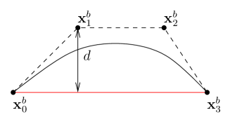
Figure 4: A cubic Bézier curve, its control polygon (dashed lines) and the coarsest approximation of the curve in red.

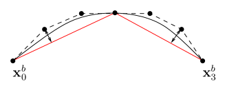
Figure 5: A first application of de Casteljau’s algorithm. The polygonal approximation in red gets closer to the control polygons (and thus to the Bézier curves).

A similar algorithm can be applied to rational Bézier splines. Most of the CAD entities can be casted as rational Bézier splines so that this optimal subdivision can be applied to most of the curves that are present in CAD models. As an example, Figure 6 presents the subdivision of a boundary using different values of the threshold parameter $\epsilon$. For the unusual cases involving non-standard parametrizations, the generic recursive sampling algorithm can be used.

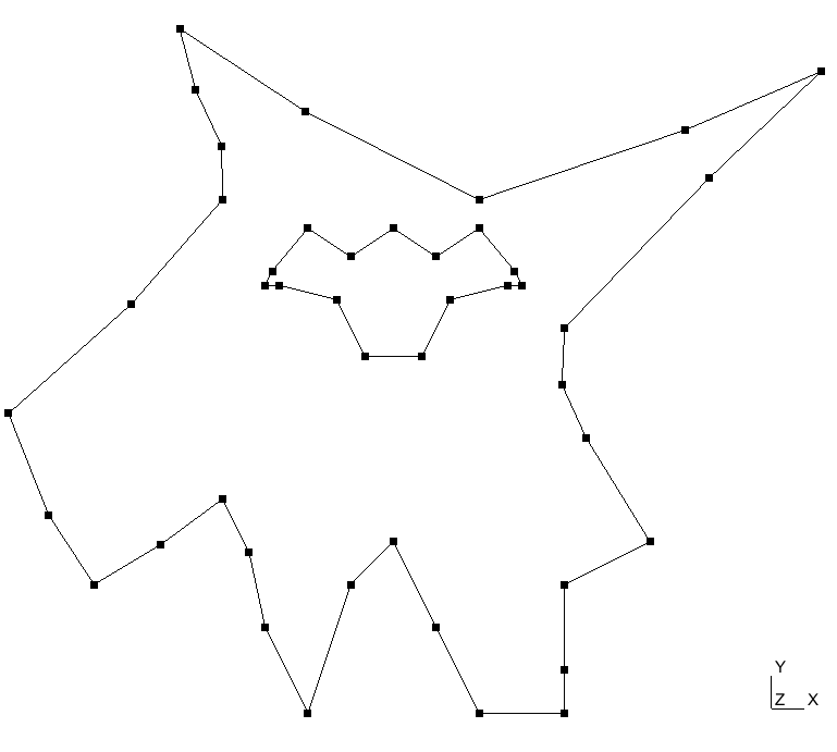
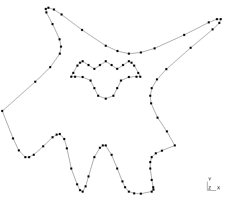
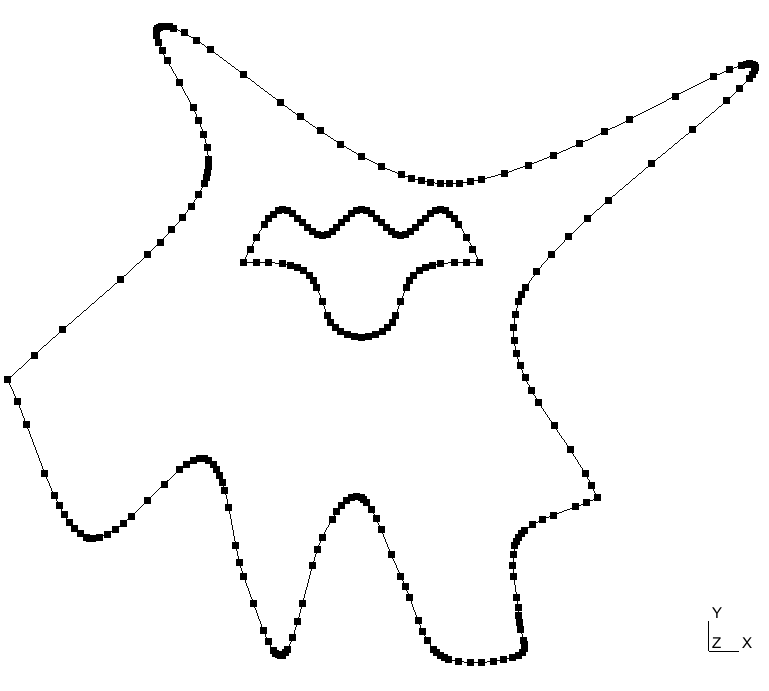
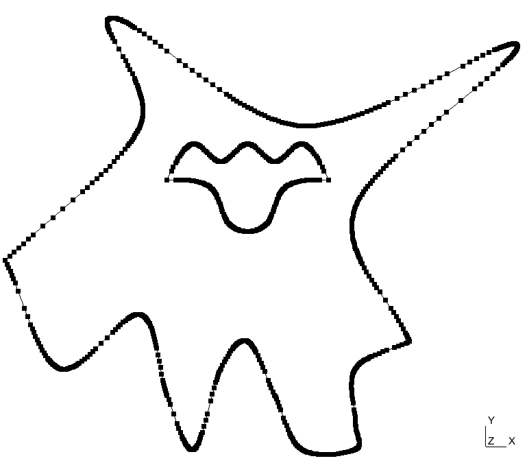
Figure 6: Adaptive subdivision of a 2D boundary with $\epsilon=5\times 10^{-2}$ (88 points), $\epsilon=10^{-2}$ (196 points), $\epsilon=10^{-3}$ (554 points), $\epsilon=10^{-4}$ (858 points)

2.2.2 Discrete distances between polygonal curves

The simplest way of approximating the distances $d_{\mathrm{H}}({\mathcal{C}},{\mathcal{C}}_{m})$ and $d_{\mathrm{F}}({\mathcal{C}},{\mathcal{C}}_{m})$ is to compute the discrete Hausdorff and Fréchet distances $\delta_{H}(M,N)$ and $\delta_{F}(M,N)$, i.e. the Hausdorff and Fréchet distances restricted to discrete point sets.

Computing $\delta_{H}(M,N)$ consist essentially in computing both Voronoi diagrams of the ${\bf{p}}_{i}$’s and of the ${\bf{q}}_{i}$’s and to find Voronoi cells of ${\bf{p}}_{i}$ that contains ${\bf{q}}_{j}$ and Voronoi cells of ${\bf{q}}_{j}$ that contains ${\bf{p}}_{i}$. Computing $\delta_{H}(M,N)$ requires ${\mathcal{O}}(m+n)\log(n+m)$ operations. In our implementation, we do not explicitly construct the Voronoi diagram. An approximate nearest neighbor algorithm [3] is used to locate closest points, leading to the same algorithmic complexity. The following result holds

$$d_{H}(M,N)\leq\delta_{H}(M,N)\leq d_{H}(M,N)+\max\{D(M),D(N)\}.$$

where $D(M)$ (resp. $D(N)$) is the maximum distance between two successive points in $M$ (resp. $N$). In Section 2.2.1, the accuracy $\epsilon$ of the polygonal representation is supposed to be much smaller than the actual distance between the CAD and the mesh in such a way that

$$|d_{H}(M,N)-d_{H}({\mathcal{C}},{\mathcal{C}}_{m})|={\mathcal{O}}(\epsilon).$$

Consequently, the discrete distance is accurate enough if and only if

$$\max\{D(M),D(N)\}<\epsilon,$$

which implies that the approximate nearest neighbor algorithm should not be applied directly to the vertices of $M$ and $N$, but to sets of points sampled at interval $\epsilon$ on these polygonal curves instead. Note that it is still useful to construct the optimal polygonal approximations $M$ and $N$ and to sample these rather than obtaining directly a dense sampling of ${\mathcal{C}}$ and ${\mathcal{C}}_{m}$, because evaluating a point of a Bézier curve is computationally much more intensive than evaluating a point of a line segment. Unfortunately, the number of points to be submitted to the approximate nearest neighbor algorithm is clearly a problem in our context, where a relative accuracy of $10^{-6}$ is often required.

The discrete Fréchet distance $\delta_{F}(M,N)$ [9] considers only positions of the “leash” where its endpoints are located at vertices of the two polygonal curves and never in the interior of an edge. The discrete Fréchet distance can be computed in polynomial time, i.e. in ${\mathcal{O}}(mn)$ operations, using a simple dynamic programming algorithm that is described in [9]. It is very difficult to find a sub-quadratic algorithm that computes the discrete Fréchet distance. We have again

$$d_{F}(M,N)\leq\delta_{F}(M,N)\leq d_{F}(M,N)+\max\{D(M),D(N)\}.$$

Computing the discrete Fréchet distance may be out of reach if massive oversampling is applied.

2.2.3 Direct distances between polygonal curves

Let us now consider the real Hausdorff and Fréchet distances between polygonal curves, that is, considering the line segments per se and not only discrete sets of points on them.

The computation of the direct Hausdorff distance between two polygonal curves is related to the Voronoi diagram of the line segments. The distance can only occur at points that are either endpoints of line segments or intersection points of the Voronoi diagram of one of the sets with a segment of the other. This observation leads us to the following quadratic algorithm for computing the direct Hausdorff distance $d_{H}(M,N)$.

• Compute the bissector of all possible pairs of segments of polygonal curve $N$. Two line segment have a bisector with up to 7 arcs (lines and parabolas). Store all arcs in a list.

• Compute the intersections of each arc with $M$.

• Compute the distance between those intersection points and $N$. The one sided Hausdorff distance is the maximum of those distances.

The Voronoi diagram of line segments could be theoretically computed in ${\mathcal{O}}((n+m)\log(n+m))$ operations [2]. Yet, it involves the computation of the whole Voronoi diagram. To our knowledge, few robust implementations of Voronoi diagrams of line segments exist [11] and no extension to higher dimensions than two has been proposed to date.

It is possible to compute the Fréchet distance $d_{F}(M,N)$ between two polygonal curves in ${\mathcal{O}}\left(mn\log(mn)\right)$ operations [2]. The algorithm is even more complex that for direct Hausdorff distance.

2.3 Geometrical error based on Taylor expansions

In the above sections, the curves ${\mathcal{C}}_{m}$ and ${\mathcal{C}}$ have been approximated by polygons, so that their relative distance can be easily and efficiently computed without any assumption about the curves. Another approach for simplifying the computation of the geometrical error is to take advantage of the fact that the high-order nodes $\text{\boldmath$x$\unboldmath}_{i}$ defining the mesh edge ${\mathcal{C}}_{m}$ are located both on ${\mathcal{C}}_{m}$ and on the model curve ${\mathcal{C}}$. A Taylor expansion of the natural parameter in the vicinity of $\text{\boldmath$x$\unboldmath}_{i}$ for each curve then provides an estimation of the geometrical error.

Assume a curve defined by $\text{\boldmath$x$\unboldmath}(t)$, $t\in[t_{1},t_{2}]$. The curvilinear abscissa $s(t)$ of a point $\text{\boldmath$x$\unboldmath}(t)$ of the curve is the length of the segment defined by parameter range $[t_{1},t]$, i.e. the length of the curve from the origin $\text{\boldmath$x$\unboldmath}(t_{1})$ to $\text{\boldmath$x$\unboldmath}(t)$:

$$s(t)=\int_{t_{1}}^{t}~{}\left\|\text{\boldmath$x$\unboldmath}_{,t}\right\|dt$$

We have $ds=\left\|\text{\boldmath$x$\unboldmath}_{,t}\right\|dt$. The arc length $s(t)$ provides the natural parametrization $\bar{\text{\boldmath$x$\unboldmath}}(s)$ of the curve:

$$\bar{\text{\boldmath$x$\unboldmath}}(s(t))=\text{\boldmath$x$\unboldmath}(t),~{}~{}t\in[t_{1},t_{2}],$$

with $\left\|\bar{\text{\boldmath$x$\unboldmath}}_{,s}\right\|=1$, where $\bar{\text{\boldmath$x$\unboldmath}}_{,s}$ is the derivative of $\bar{\text{\boldmath$x$\unboldmath}}$ with respect to $s$. The unit tangent vector to the curve is computed as

$${\bf{t}}=\bar{\text{\boldmath$x$\unboldmath}}_{,s}={\text{\boldmath$x$\unboldmath}_{,t}\over\|\text{\boldmath$x$\unboldmath}_{,t}\|}.$$ (4)

The curvature vector ${\bf{k}}$ of the curve at a point $x$ can be defined as the amplitude of the variations of the unit tangent ${\bf{t}}$ along the curve. The vector ${\bf{k}}={\bf{t}}_{,s}$ is obviously orthogonal to ${\bf{t}}$ because ${\bf{t}}$’s amplitude is equal to one along $s$. We have

$${\bf{k}}=\bar{\text{\boldmath$x$\unboldmath}}_{,ss}=\frac{1}{\left\|\text{\boldmath$x$\unboldmath}_{,t}\right\|^{3}}\left(\text{\boldmath$x$\unboldmath}_{,tt}\left\|\text{\boldmath$x$\unboldmath}_{,t}\right\|-\text{\boldmath$x$\unboldmath}_{,t}\frac{\text{\boldmath$x$\unboldmath}_{,t}\cdot\text{\boldmath$x$\unboldmath}_{,tt}}{\|\text{\boldmath$x$\unboldmath}_{,t}\|}\right).$$

It is thus possible to approximate the curve with a Taylor expansion of $\bar{\text{\boldmath$x$\unboldmath}}$ around $s_{0}=s(t_{0})$ at second order as

$$\bar{\text{\boldmath$x$\unboldmath}}(s_{0}+s)=\bar{\text{\boldmath$x$\unboldmath}}(s_{0})+s\left.{\bf{t}}\right|_{s_{0}}+\frac{s^{2}}{2}\left.{\bf{k}}\right|_{s_{0}}+{\mathcal{O}}(s^{3}).$$ (5)

Applying this expansion for a mesh edge ${\mathcal{C}}_{m}$ and the corresponding model curve ${\mathcal{C}}$, the geometrical error between both curves can be estimated near each of their common points $\text{\boldmath$x$\unboldmath}_{i}$ as

$$\delta^{i}_{T,L}=\left\|h({\bf{t}}_{m}-{\bf{t}})\right\|$$

for a linear approximation and

$$\delta^{i}_{T,Q}=\left\|h({\bf{t}}_{m}-{\bf{t}})+{h^{2}\over 2}({\bf{k}}_{m}-{\bf{k}})\right\|$$

for a quadratic approximation. In these expressions, the unit tangent vector ${\bf{t}}_{m}$ (resp. ${\bf{t}}$) and the curvature vector ${\bf{k}}_{m}$ (resp. ${\bf{k}}$) is computed on ${\mathcal{C}}_{m}$ and (resp. ${\mathcal{C}}$) at point $\text{\boldmath$x$\unboldmath}_{i}$, and $h$ is proportional to a “local edge length” computed from the Jacobian of ${\mathcal{C}}_{m}$. The derivatives of $\text{\boldmath$x$\unboldmath}_{m}$ required to compute ${\bf{t}}_{m}$ and ${\bf{k}}_{m}$ can be easily obtained from Eq. (1). For the vectors ${\bf{t}}$ and ${\bf{k}}$ related to the model curve ${\mathcal{C}}$, the derivatives of $x$ are provided by the CAD model. The geometrical error for the whole mesh edge ${\mathcal{C}}_{m}$ can then be computed as

$$\delta_{T}=\left(\sum_{i=0}^{p}{d^{i}_{T}}^{2}\right)^{\frac{1}{2}}.$$

2.4 A simple example

In order to illustrate the different estimates of the geometrical error described above, we consider the simple case of a particular Lamé curve:

$$y=\frac{1}{2}\left(1-x^{4}\right)^{\frac{1}{4}},\;\;x\in[0,1].$$

The geometrical model is a Bézier spline representing this curve with negligible error (see Fig. 7). The spline is parametrized with a variable $u\in[0,1]$.

A quadratic mesh edge is built to approximate the model curve. Its end vertices are fixed at the extremities of the curve (i.e. $u=0$ and $u=1$), and we explore the values of $\delta_{F}$, $\delta_{H}$ and $\delta_{T}$ for different locations of the high-order node on the model curve. In particular, we consider 100 locations in the range $u\in[0.2,0.68]$, where the Jacobian of the edge is positive (i.e. the mesh is valid).

The evolution of the discrete Hausdorff distance $\delta_{H}$ with the high-order node location is shown in Fig. 8 for different values of the accuracy threshold $\epsilon$. A value of $\epsilon=10^{-3}$ seems to yield sufficient accuracy for this curve. In this particular case, the discrete Fréchet distance $\delta_{F}$ is equal to the discrete Hausdorff distance $\delta_{H}$.

Fig. 9 shows the quantities $\delta_{H}=\delta_{F}$ and $\delta_{T}$ normalized by their respective maximum value, so that they can be compared to each other. Although both curves are qualitatively similar, they do not reach a minimum for the same high-order node location ($u=0.617$ for $\delta_{H}$ and $u=0.573$ for $\delta_{T}$), which can be visualized in Fig. 7. Moreover, it clearly appears that the Taylor-based geometrical error $\delta_{T}$ is a continuously differentiable function of the high-order node position, while the the Hausdorff and the Fréchet distances $\delta_{H}$ and $\delta_{F}$ are not differentiable everywhere, in particular at their minimum.

The approximate CPU time for one distance evaluation, measured on a recent laptop computer, is about $3.0\cdot 10^{-2}\;\textrm{s}$ for $\delta_{F}$, and $2.4\cdot 10^{-3}\;\textrm{s}$ for $\delta_{H}$ with $\epsilon=10^{-3}$, whereas it is only $1.1\cdot 10^{-6}\;\textrm{s}$ for $\delta_{T}$. Given its continuously differentiable nature and its low computational cost, the Taylor-based geometrical error estimate $\delta_{T}$ is clearly much more appropriate than the other distances for an optimization procedure such as the one described in Sec. 3.

Figure 7: Geometrical model representing a Lamé curve (thick blue line) and corresponding quadratic mesh edges minimizing $\delta_{H}=\delta_{F}$ (red thin line) and $\delta_{T}$ (green thin line).

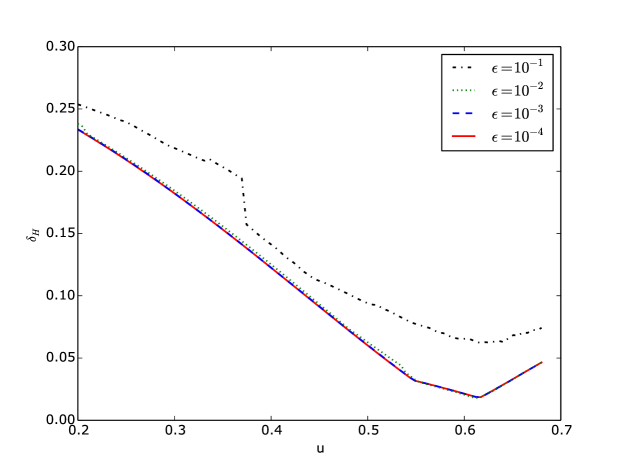
Figure 8: Case of a Lamé curve: discrete Hausdorff distance $\delta_{H}=\delta_{F}$ for the quadratic mesh edge as a function of the position $u$ of the high-order node on the geometrical model.

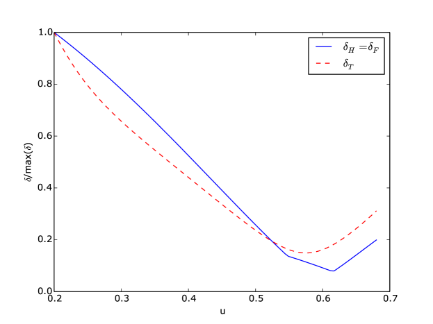
Figure 9: Case of a Lamé curve: quantities $\delta_{H}=\delta_{F}$ and $\delta_{T}$, normalized by their maximum value, for the quadratic mesh edge as a function of the position $u$ of the high-order node on the geometrical model.

3 Mesh optimization

In a recent paper [24], a technique that allows to untangle high order/curvilinear meshes is presented. The technique makes use of unconstrained optimization where element Jacobians are constrained to lie in a prescribed range through moving log-barriers. The untangling procedure starts from a possibly invalid curvilinear mesh and moves mesh vertices with the objective of producing elements that all have bounded Jacobians. Bounds on Jacobians are computed using results of papers [12, 13]. In what follows, we extend the optimization procedure in charge of untangling the invalid elements in order to take into account the geometrical error $\delta_{T}$.

The procedure described in Ref. [24] consists in solving a sequence of minimization problems, where the objective function $f(\text{\boldmath$x$\unboldmath}_{i})$ is composed of two parts ${\mathcal{E}}$ and ${\mathcal{F}}\epsilon$:

$$f={\mathcal{E}}+{\mathcal{F}}_{\epsilon}$$

Here $\text{\boldmath$x$\unboldmath}_{i}$ is the position of node $i$. For a node located on a boundary, it is possible to work with the parametric coordinate(s) of the node on the geometrical model entity given by the CAD model. As the scale of the parametric coordinate can differ significantly from the scale of the physical coordinates, preconditioning may then be required for the Conjugate Gradient to converge properly.

The first part ${\mathcal{E}}$ relies on the assumption that the method is provided with a straight-sided mesh of high quality. This mesh has potentially been defined to satisfy multiple criteria, such as a predetermined size field, or anisotropic adaptation. The conversion of such meshes to high order is expected to preserve as much as possible all these features. Therefore, the nodes shall be kept as close as possible to their initial location in the straight sided mesh. In this work, the definition of ${\mathcal{E}}$ is the one of [24] i.e.

$${\mathcal{E}}(\text{\boldmath$x$\unboldmath}_{i})=\frac{K_{\mathcal{E}}}{L^{2}}\sum_{i}\left\|\text{\boldmath$x$\unboldmath}_{i}-\text{\boldmath$X$\unboldmath}_{i}\right\|^{2}$$ (6)

with $\text{\boldmath$X$\unboldmath}_{i}$ the position of the node $i$ in the straight-sided mesh, $K_{\mathcal{E}}$ a non dimensional constant and $L$ a characteristic size of the problem.

The second part ${\mathcal{F}}$ of the functional controls the positivity of the Jacobian. A $\log$ barrier [24] prevent Jacobians from becoming too small:

$${\mathcal{F}}_{\epsilon}(\text{\boldmath$x$\unboldmath}_{i})=\sum_{e}\sum_{l}F^{e}_{l}(\text{\boldmath$x$\unboldmath}_{i},\epsilon)$$

with $l$ iterating on all coefficients $B^{e}_{l}$ of the Bézier expansion of the Jacobian of $e$ and where

$$F^{e}_{l}(\text{\boldmath$x$\unboldmath}_{i},\epsilon)=\left[\log\left(\frac{B^{e}_{l}(\text{\boldmath$x$\unboldmath}^{e})-\epsilon J^{e}_{0}}{J^{e}_{0}-\epsilon J^{e}_{0}}\right)\right]^{2}+\left(\frac{B^{e}_{l}(\text{\boldmath$x$\unboldmath}^{e})}{J^{e}_{0}}-1\right)^{2}$$ (7)

is the log barrier function defined in such a way that ${\mathcal{F}}$ blows up when $B^{e}_{l}/J^{e}_{0}\rightarrow\epsilon$, but still vanishes when $B^{e}_{l}=J^{e}_{0}$. In this expression, $\text{\boldmath$x$\unboldmath}^{e}$ is the vector gathering the positions $\text{\boldmath$x$\unboldmath}_{i}$ of all nodes $i$ belonging to element $e$, and $J^{e}_{0}$ is the constant straight sided Jacobian of $e$.

The value of $K_{\mathcal{E}}$ has little influence on results. The presence of ${\mathcal{E}}$ prevents the problem from being under-determined, and it orients the optimization procedure towards a solution that tends to preserve the straight-sided mesh, but it is clearly dominated by ${\mathcal{F}}_{\epsilon}$ when invalid elements exist in the domain.

A Conjugate Gradient algorithm is used to minimize the objective function $f$ with respect to the node positions $\text{\boldmath$x$\unboldmath}_{i}$ for a fixed value of the log barrier parameter $\epsilon$. A sequence of such minimization problems is solved, in between which the $\epsilon$ is progressively increased, so that the Jacobian of all elements is forced to exceed a user-defined target value.

In the present work, the procedure described above is followed in a first step. In a second step, a similar procedure is used, albeit with an objective function f taking into account the geometrical model:

$$f={\mathcal{E}}+{\mathcal{F}}_{\epsilon}+{\mathcal{D}}_{\epsilon^{\prime}}$$

The third part ${\mathcal{D}}_{\epsilon^{\prime}}$ of the functional controls the error $\delta_{T}$ between the mesh and the geometrical model. Again, a log barrier is used:

$${\mathcal{D}}_{\epsilon^{\prime}}(\text{\boldmath$x$\unboldmath}_{i})=K_{\mathcal{D}}\sum_{b}D^{b}(\text{\boldmath$x$\unboldmath}_{i},\epsilon)$$

with $b$ iterating on all boundary mesh edges and

$$D^{e}_{l}(\text{\boldmath$x$\unboldmath}_{i},\epsilon^{\prime})=\left[\log\left(\frac{\delta_{T}^{b}(\text{\boldmath$x$\unboldmath}^{b})-\epsilon\delta_{0}}{\delta_{0}-\epsilon\delta_{0}}\right)\right]^{2}+\left(\frac{\delta_{T}^{b}(\text{\boldmath$x$\unboldmath}^{b})}{\delta_{0}}\right)^{2}$$

where $\delta_{T}^{b}$ is the is the geometrical error $\delta_{T}$ for the boundary mesh edge $b$, and $\delta_{0}$ is a target value for $\delta_{T}^{b}$. The vector $\text{\boldmath$x$\unboldmath}^{b}$ collects the positions $\text{\boldmath$x$\unboldmath}_{i}$ of all nodes $i$ belonging to the boundary mesh edge $b$. Derivatives of $\delta_{T}$ with respect to $\text{\boldmath$x$\unboldmath}_{i}$ are computed using finite differences.

In this second step, ${\mathcal{F}}_{\epsilon}$ is used as a fixed log barrier (constant $\epsilon$) that is meant to prevent the Jacobian of elements to fall back below the target value reached in the first step. On the contrary, ${\mathcal{D}}_{\epsilon^{\prime}}$ is a moving log barrier where the parameter $\epsilon^{\prime}$ is iteratively updated to drive the geometrical error $\delta_{T}$ towards its target value. The parameter $K_{\mathcal{D}}$ reflects the weight given to the geometrical error contribution with respect to the contribution of the Jacobians. In this work, we typically choose values around $K_{\mathcal{D}}=0.1$.

4 Examples

4.1 NACA0012

We consider the classical geometry of the NACA0012 airfoil with unit chord length. Sequences of 6 triangular meshes are generated, where the airfoil is discretized by $4$, $6$, $10$, $18$, $34$ and $66$ elements respectively, for a total of $244$, $298$, $436$, $546$, $832$ and $1178$ elements in each mesh. The first sequence consists of linear meshes. Two others are composed of quadratic meshes resulting from the optimization procedure described in Section 3: one is optimized for element validity only, while the other also minimizes the geometrical error. The last two sequences are made up of cubic meshes generated in the same manner as the quadratic ones.

Figure 10 shows how the geometrical error $\delta_{T}$ and the model-to-mesh Hausdorff distance $\delta_{H}$ evolve with the mesh size. In meshes optimized for validity only, both $\delta_{T}$ and $\delta_{H}$ clearly decrease with decreasing mesh size, but most meshes are too coarse to yield the optimal convergence rate. However, minimizing the geometrical error $\delta_{T}$ reduces both $\delta_{T}$ and $\delta_{H}$ of at least one order of magnitude in most cases. Geometrically-optimized quadratic meshes are even more accurate than valid cubic meshes. The geometrical optimization is most beneficial for coarser meshes, which lie precisely the range of mesh size where refining brings less geometrical accuracy. For fine cubic meshes, the improvement is less significant: meshes optimized for validity only converge at near asymptotic rate for both while $\delta_{T}$ and $\delta_{H}$, while the convergence rate with meshes optimized for both validity and geometrical accuracy is not improved (or even reduced for $\delta_{T}$). Thus, optimizing meshes with respect to $\delta_{T}$ may be particularly interesting with numerical schemes of very high order running on coarse meshes, where it may yield a suitable geometrical approximation of the model without unnecessary mesh refinement.

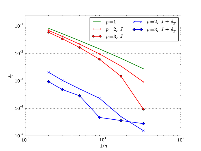
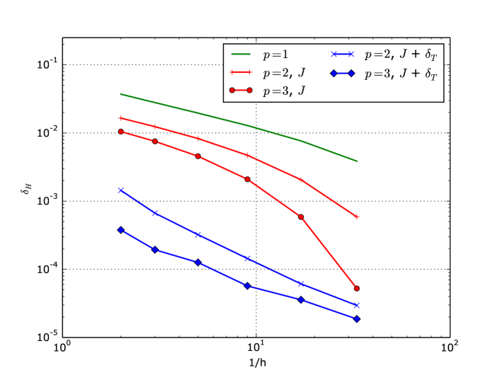
Figure 10: Geometrical error $\delta_{T}$ (top) and model-to mesh Hausdorff distance $\delta_{H}$ (bottom) for the NACA0012 profile: linear meshes ($p=1$) as well as quadratic ($p=2$) and cubic ($p=3$) meshes optimized either for element validity only ($J$) or for both element validity and geometrical error ($J+\delta_{T}$).

Examples of meshes are shown in Figures 11 and 12. In geometrically-optimized meshes, the high-order nodes located on the boundary are clearly moved along the CAD curve to minimize $\delta_{T}$, while they remain in the middle of corner nodes when validity only is considered. In coarse meshes, some elements need to be strongly deformed to satisfy both geometrical and validity criteria, which may affect the simulations adversely. Indeed, highly distorted elements are known to harm the accuracy of finite element approximations [6]. They may also deteriorate the conditioning of the spatial discretization operator, with negative impact on time integration [23]. Moreover, a correct integration of polynomial quantities on such elements may require costly higher-order quadrature rules. Fortunately, the effect is less pronounced in finer meshes.

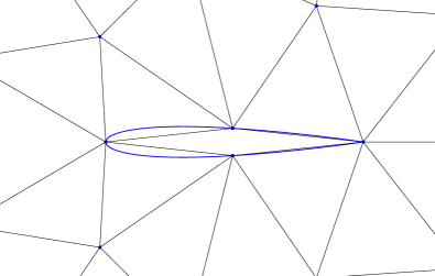
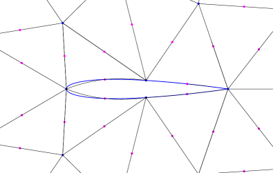
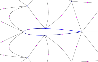
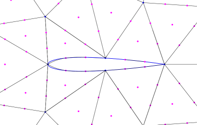
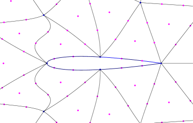
Figure 11: Coarsest meshes of the NACA0012 profile. Top: linear mesh. Center: quadratic meshes optimized for validity only (left) and for validity as well as geometrical error (right). Bottom: cubic meshes optimized for validity only (left) and for validity as well as geometrical error (right).

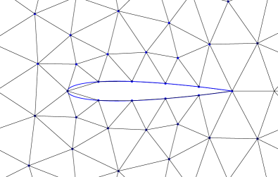
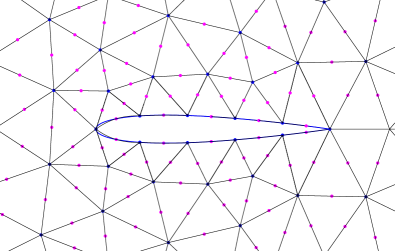
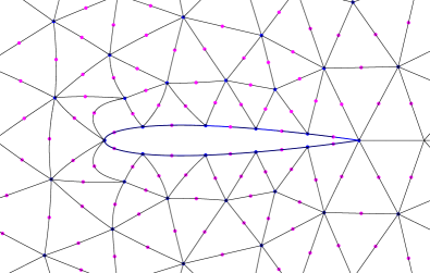
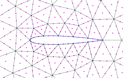
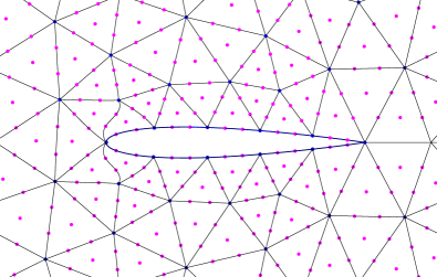
Figure 12: Medium-size meshes of the NACA0012 profile. Top: linear mesh. Center: quadratic meshes optimized for validity only (left) and for validity as well as geometrical error (right). Bottom: cubic meshes optimized for validity only (left) and for validity as well as geometrical error (right).

In order to illustrate the impact of the geometrical accuracy on simulations, computations solving the Euler flow around the NACA0012 airfoil at Mach number $M=0.5$ and $3^{\circ}$ angle-of-attack have been carried out. A high-order ($p=6$ i.e. sixth-order polynomials) discontinuous Galerkin scheme was used for the spatial discretization, and steady-state solutions were obtained through a pseudo-time approach involving a backward Euler scheme in combination with a Newton-Krylov solver. Slip wall conditions are imposed on the airfoil and characteristic-based free-stream boundary conditions are used at the far-field boundary of the domain.

Results for meshes in which the airfoil is discretized with 34 elements are shown in Figure 13. Unsurprisingly, the numerical method does not converge properly with the linear mesh, and the residual cannot be decreased by more than two orders of magnitude. The density field is clearly different from the expected solution. With the quadratic mesh optimized for validity only, the airfoil is represented more accurately, but the corresponding solution still exhibits spurious oscillations and flow features near corner nodes on the wall boundary, where the representation of the airfoil is not smooth. A drop of four orders of magnitude in residual is achieved in 26 pseudo-time iterations. With the geometrically-optimized mesh however, the computation converges towards the expected smooth solution in 19 pseudo-time iterations. In this purely inviscid test case, the increased boundary smoothness resulting from the minimization of $\delta_{T}$ is instrumental in converging towards the exact solution without spurious entropy generation at the boundary. Moreover, the geometrically-optimized quadratic mesh represents the model so accurately that it is meaningless to use a higher-order mesh, as the Hausdorff distance $\delta_{H}\approx 4\cdot 10^{-5}$ is probably already lower than the manufacturing tolerance of the airfoil.

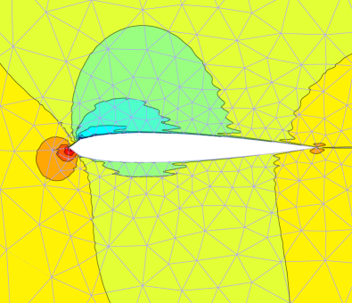
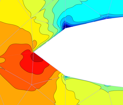
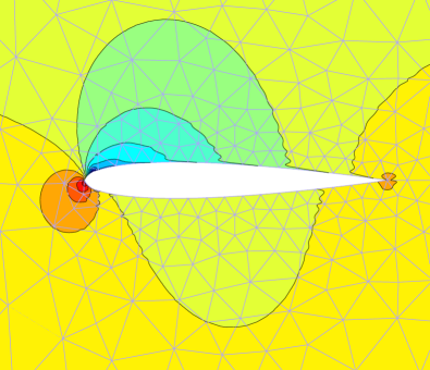
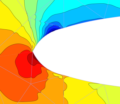
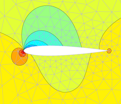
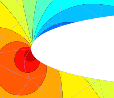
Figure 13: Density field for the NACA0012 case: flow around the airfoil (left column) and zoom around the leading edge (right column). Top row: results with a linear mesh. Middle row: results with a quadratic mesh optimized for validity only. Bottom row: results with a quadratic mesh optimized for both validity and geometrical accuracy.

4.2 Rattray island

We consider now an ocean modelling application focusing on the Rattray island, that is located in the Great Barrier Reef near Australia. Simulations have been performed, in which the shallow water equations are solved without diffusion nor Coriolis force. The water depth at rest is uniform and equal to $25\,\textrm{m}$. Slip wall conditions are imposed on the island coast and the lateral sides of the domain. At the upstream and downstream sides of the domain, uniform free-stream conditions are prescribed with a velocity corresponding to a Froude number of $Fr=0.02$, which is representative of the tidal stream [25]. The island, that has a length of about $1350\,\textrm{m}$, is oriented at $60^{\circ}$ compared to the free stream. In this setup, there is no source of vorticity, and the ideal solution is a steady irrotational flow. A view of the domain and the solution is given in Figure 14.

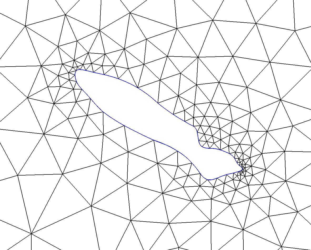
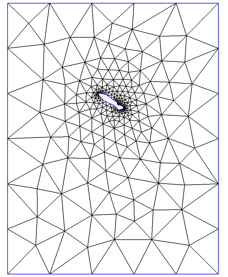
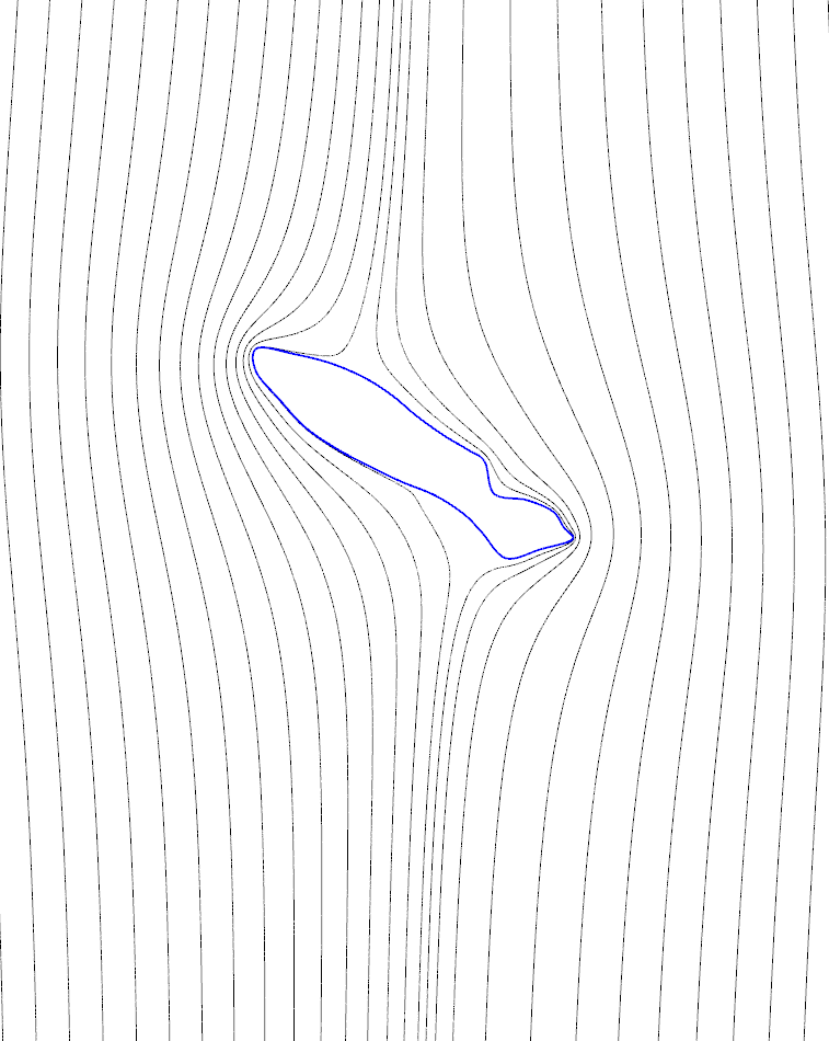
Figure 14: Rattray test case: general view of the computational domain and quadratic mesh (bottom left), zoom on the mesh around the island (top) and streamlines of the ideal solution in the vicinity of the island (right).

A quadratic mesh of $596$ elements with higher density near curved boundaries is generated. This mesh is already valid without optimization. A second mesh is obtained by minimizing $\delta_{T}$ according to the procedure described in Section 3. Figure 15 shows a comparison of both meshes at the tips of the island. The mesh boundaries of both meshes look very similar. Indeed, the model-to-mesh Hausdorff distance for the original mesh ($\delta_{H}=1.45\,\textrm{m}$) is not significantly different from the one for the optimized mesh ($\delta_{H}=0.66\,\textrm{m}$). This is due to the fact that the geometry is already well resolved by the unoptimized mesh. However, a close examination of Figure 15 reveals that the boundary of the unoptimized mesh is not perfectly smooth at element corners, while the optimized mesh looks better in this respect.

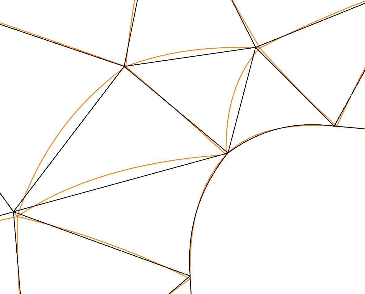
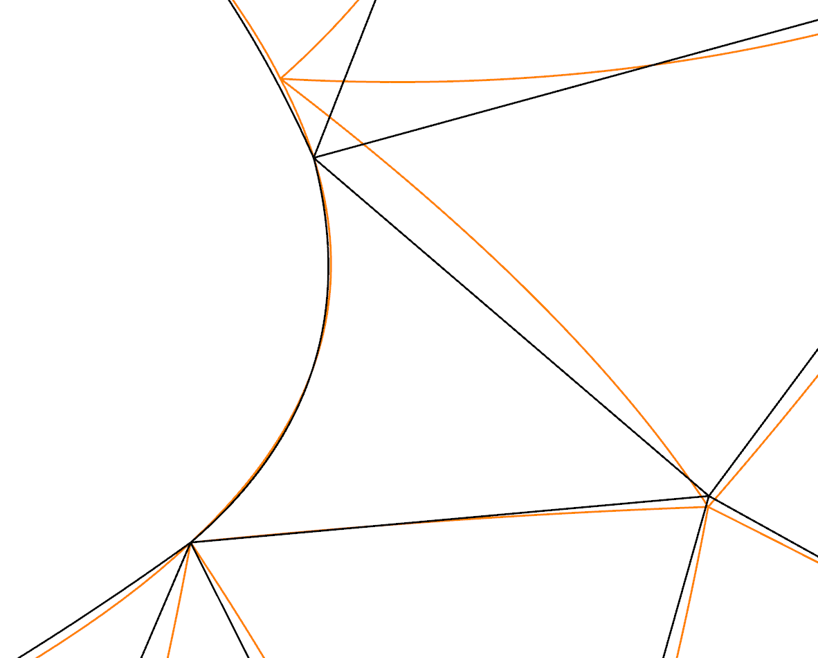
Figure 15: Rattray test case: comparison between the original quadratic mesh (black) and the geometrically-optimized mesh (orange) at the upstream tip (left) and the downstream tip (right) of the island.

Even though the improvement in the Taylor-based geometrical error is not necessarily impressive ($\delta_{T}=2.19\,\textrm{m}$ for the unoptimized mesh against $\delta_{T}=0.37\,\textrm{m}$ for the optimized one), the impact on the solution is important. Simulations were performed with the same numerical method as in Section 4.1. Figure 16 compares the results between both meshes. With the unoptimized mesh, vortices are shed from the downstream tip of the island, preventing the flow from reaching steady-state, while a drop of 4 orders of magnitude in residuals can be achieved with the optimized mesh, leading to a nearly potential solution. This test case shows, even more than in the NACA0012 case, that the gain in boundary smoothness brought by the geometrical optimization is crucial to obtain the correct solution in some problems.

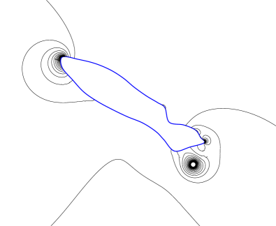
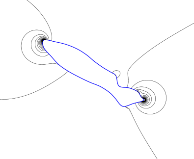
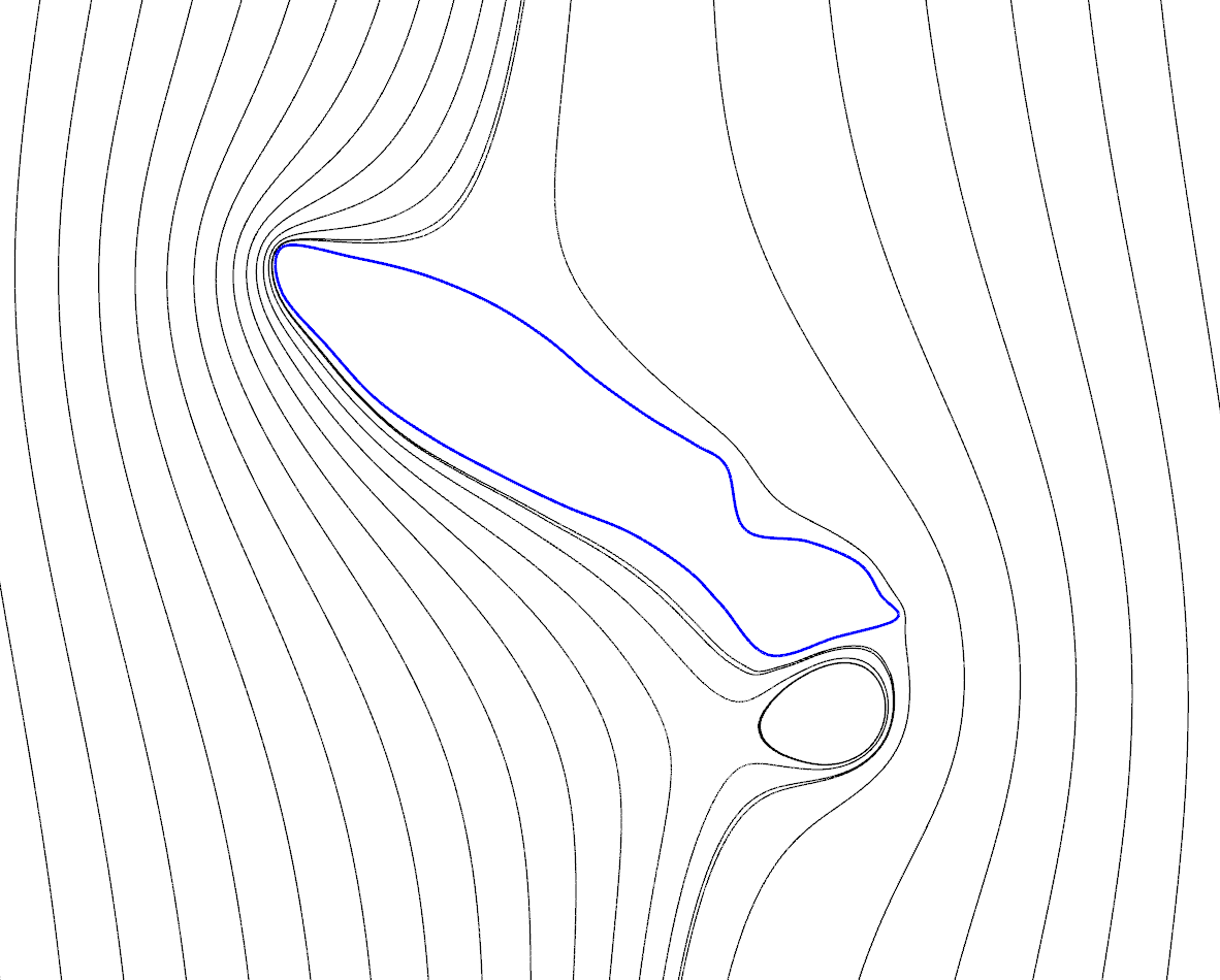
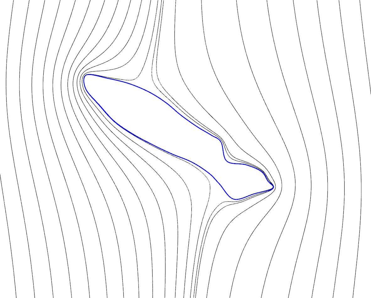
Figure 16: Rattray test case: contours of the sea surface elevation (upper row) and streamlines (bottom row) at $t=2100\,\textrm{s}$. Results obtained with the original quadratic mesh (left column) and with the geometrically-optimized mesh (right column).

4.3 High-lift airfoil

In this section, we apply the methods described in Section 3 to an acoustic application involving a high-lift airfoil. The geometry is a 3-element airfoil based on the RA16SC1 profile, with the slat and flap deflected by $30^{\circ}$ and $20^{\circ}$ respectively. The chord of the main element is $480\,\textrm{mm}$, and the computational domain is a disc of radius $1\,\textrm{m}$ centered on a point P located close to the trailing edge. The acoustic excitation consists of a monopole source placed at point P, with an amplitude of $1\,\textrm{Pa}$ and frequency of $7816\,\textrm{Hz}$. The computational domain is shown in Figure 17.

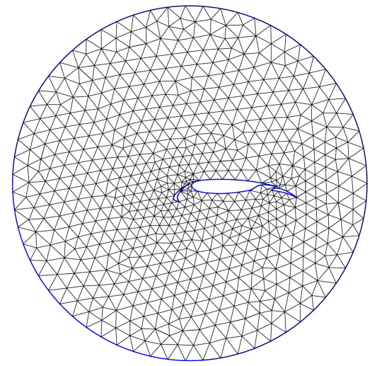
Figure 17: Acoustics test case: computational domain and medium-size quadratic mesh (left).

Simulations are performed with a discontinuous Galerkin nodal scheme for the space discretization, and the standard fourth-order four-stage Runge-Kutta integrator in time. Slip wall conditions are imposed on the airfoil, while characteristic-based non-reflecting boundary conditions are prescribed in the far field. The monopole is modeled by a Gaussian pressure perturbation of half-width $3\,\textrm{mm}$. Simulation are run until a periodic regime is reached. A reference solution is obtained through a computation on a fine grid.

Two sets of triangular meshes are generated, one composed of medium-size meshes ($1617$ elements) and one composed of coarse meshes ($296$ elements). Each set consists of a linear mesh, the corresponding quadratic mesh optimized for element validity only and the corresponding quadratic mesh optimized for both validity and geometrical accuracy. Details of the meshes around the slat and the leading edge of the main component, where the boundaries influence most the acoustic field, are plotted in Figure 18.

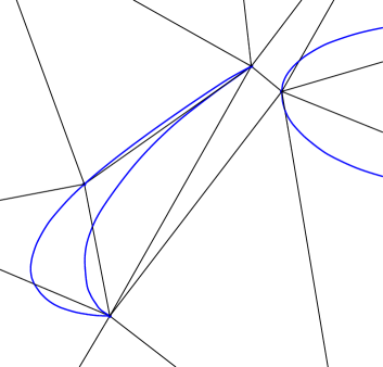
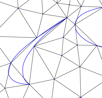
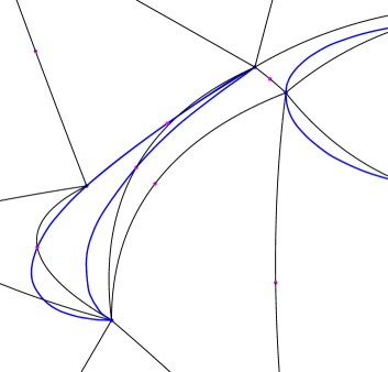
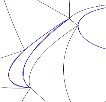
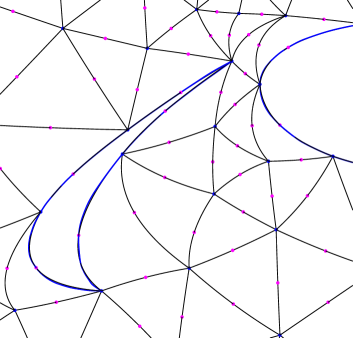
Figure 18: Acoustic test case: details of the mesh around the slat and the leading edge of the main component for the coarse meshes (left column) and the medium-size meshes (right column). Linear meshes (top row), quadratic meshes optimized for geometry only (middle row) and quadratic meshes optimized for both validity and geometrical accuracy (bottom row).

It is obvious that the coarse quadratic mesh optimized for validity only represents the model very poorly, while the minimization of the geometrical error yields a fairly accurate and smooth approximation of the airfoil. In the region of the computational domain shown in Figure 18, the geometrical optimization decreases the discrete model-to-mesh Hausdorff distance $\delta_{H}$ by a factor 7 approximately ($\delta_{H}=9.3\,\textrm{mm}$ to $\delta_{H}=1.3\,\textrm{mm}$), and the geometrical error $\delta_{T}$ drops by a factor 8 ($\delta_{T}=15.5\,\textrm{mm}$ to $\delta_{T}=1.8\,\textrm{mm}$). Above all, a close examination of mesh optimized for validity only at the trailing edge of the slat shows that the mesh edge on the lower side of the profile crosses the edge representing the upper side: even though the mesh is valid in the finite element sense, it is physically incorrect. On the contrary, a simulation with the coarse quadratic mesh optimized for geometrical accuracy can give an acceptable solution, provided that the spatial discretization is of sufficiently high order. In the present case, simulations with a 10${}^{\textrm{th}}$-order discontinuous Galerkin scheme were slightly more dissipative than the reference computation on a fine mesh (see Figure 19).

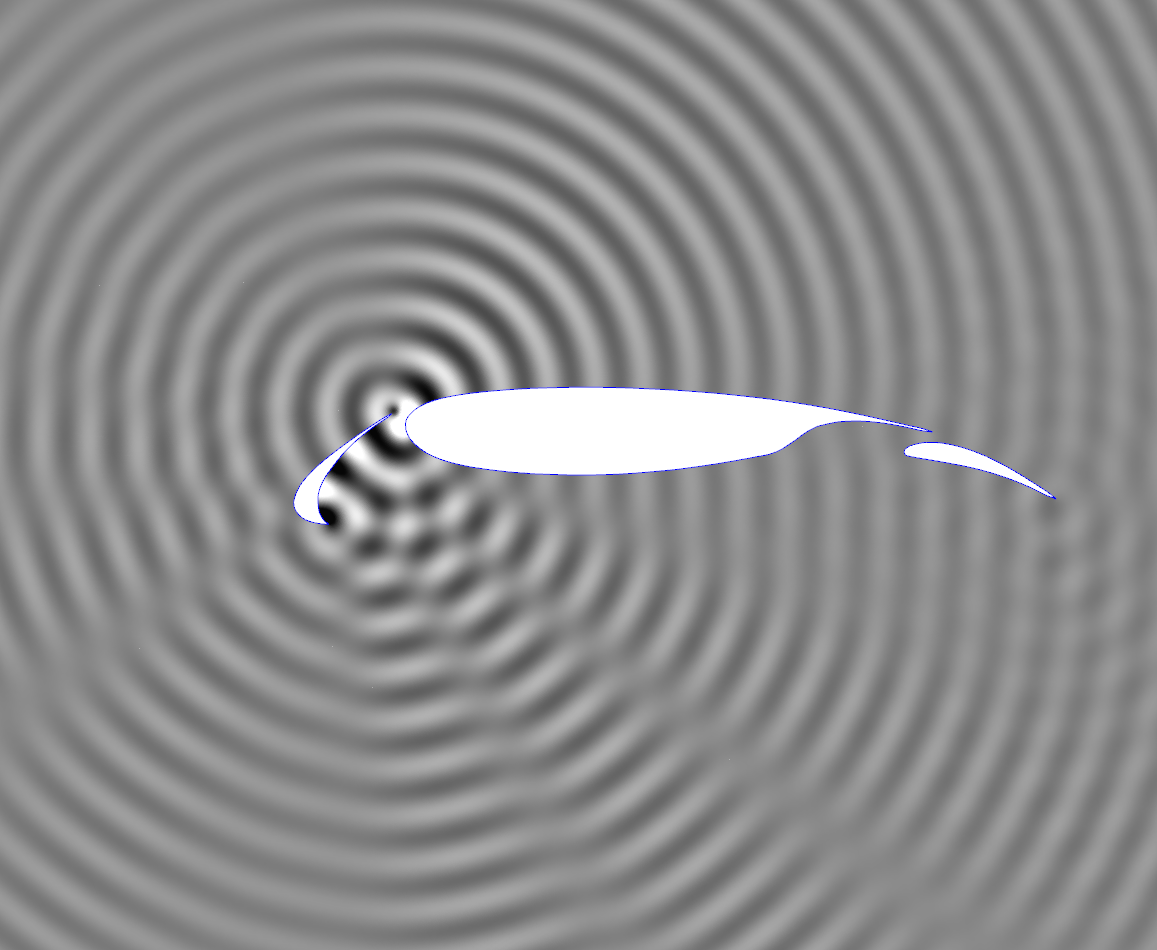
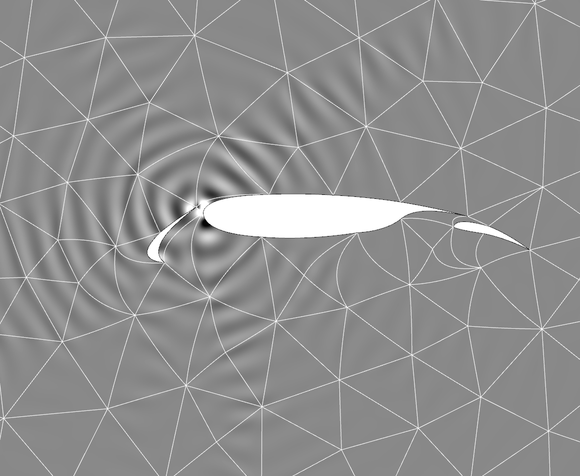
Figure 19: Acoustics test case: acoustic pressure field at final time for the reference solution (left) and the solution obtained on the coarse quadratic mesh optimized for geometrical accuracy (right).

The difference between both quadratic medium-size meshes is less spectacular, as seen in Figure 18: $\delta_{H}$ decreases by a factor 4 ($2.5\,\textrm{mm}$ to $0.6\,\textrm{mm}$) and $\delta_{T}$ by a factor of 5 ($3.8\,\textrm{mm}$ to $0.8\,\textrm{mm}$) with geometrical optimization. Simulations are run with these meshes, and the RMS acoustic pressure $p_{\textrm{RMS}}$ is measured over the last 6 oscillation periods along a circle of radius $750\,\textrm{mm}$ centered at point P. The results are expressed in terms of Sound Pressure Level as $\textrm{SPL}=20\,\log(p_{\textrm{RMS}}/p_{\textrm{ref}})$, where $p_{\textrm{ref}}=2\cdot 10^{-5}\,\textrm{Pa}$. Figure 20 shows that the effect of the geometrical optimization impacts significantly the accuracy of the sound directivity.

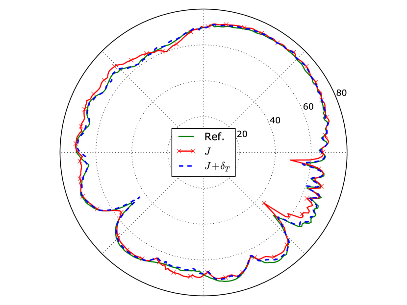
Figure 20: Acoustics test case: sound directivity expressed in terms of Sound Pressure Level (in dB) for the reference solution, as well as the solutions obtained with quadratic medium-size meshes optimized for validity only ($J$) and for both validity and geometrical accuracy ($J+\delta_{T}$).

5 Extension to three-dimensional meshes

In the same manner as described in Section 2 for curves, it is possible to define a geometrical error for a surface mesh element ${\mathcal{S}}_{m}$ approximating a model surface ${\mathcal{S}}$. At each of interpolation point $\text{\boldmath$x$\unboldmath}_{i}$ where both surfaces coincide, a first-order estimation of the geometrical error is:

$$\delta^{i}_{T}=\left\|h({\bf{n}}_{m}-{\bf{n}})\right\|.$$

where ${\bf{n}}_{m}$ represents the unit normal to ${\mathcal{S}}_{m}$ and ${\bf{n}}$ represents the unit normal to ${\mathcal{S}}$. Here, $h$ is proportional to the square root of a “local surface element area”, determined from the Jacobian of ${\mathcal{S}}_{m}$. The geometrical error $\delta_{T}$ for the surface mesh element can then be computed from all the $\delta^{i}_{T}$ in the element. It is then possible to use the optimization process presented in Section 3 in order to obtain a better representation of the model surfaces by the boundary of a 3D volume mesh.

In order to illustrate the potential of this approach for 3D meshes, we apply the method to the case of a wing made from an extruded NACA0012 profile of unit chord length. Fig. 21 shows a coarse mesh of $847$ tetrahedra in two versions, namely one optimized for validity only and one optimized for both validity and geometrical accuracy. As in the 2D case, the smoothness of the mesh boundary at the leading edge is significantly improved by the minimization of $\delta_{T}$, and the approximation of the airfoil seems to be more accurate. The geometrical error $\delta_{T}$ is indeed decreased by more than an order of magnitude ($0.16$ to $0.012$).

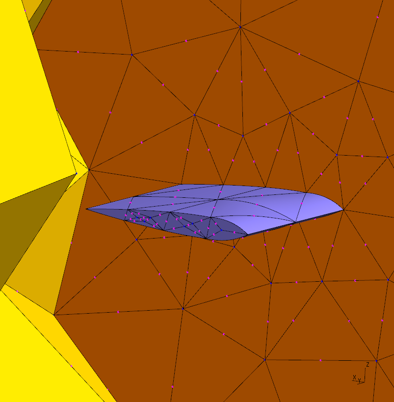
Figure 21: Mesh of the 3D NACA0012 geometry optimized for validity only (left) and for both validity and geometrical accuracy (right).

Another example is the case of an ONERA M6 wing of chord length of $810$ at wing root, illustrated in Figure 22. A coarse quadratic volume mesh of $11851$ terahedra is generated, then optimized for validity only on one hand, and for both validity and geometrical accuracy on the other hand. The geometrical error $\delta_{T}$ is reduced from $40$ to $15$ by the geometric optimization. The representation of the leading edge is clearly improved, particularly where it merges with the tip surface of the wing.

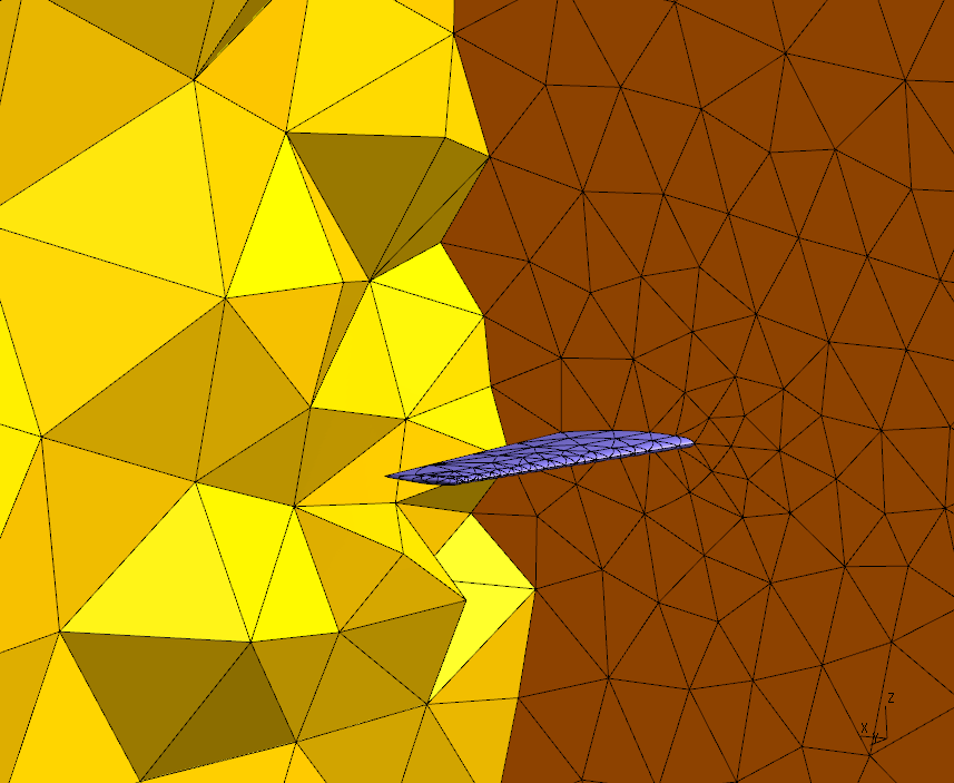
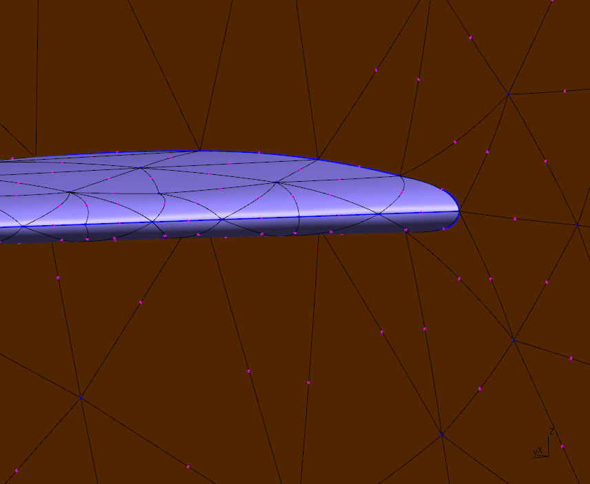
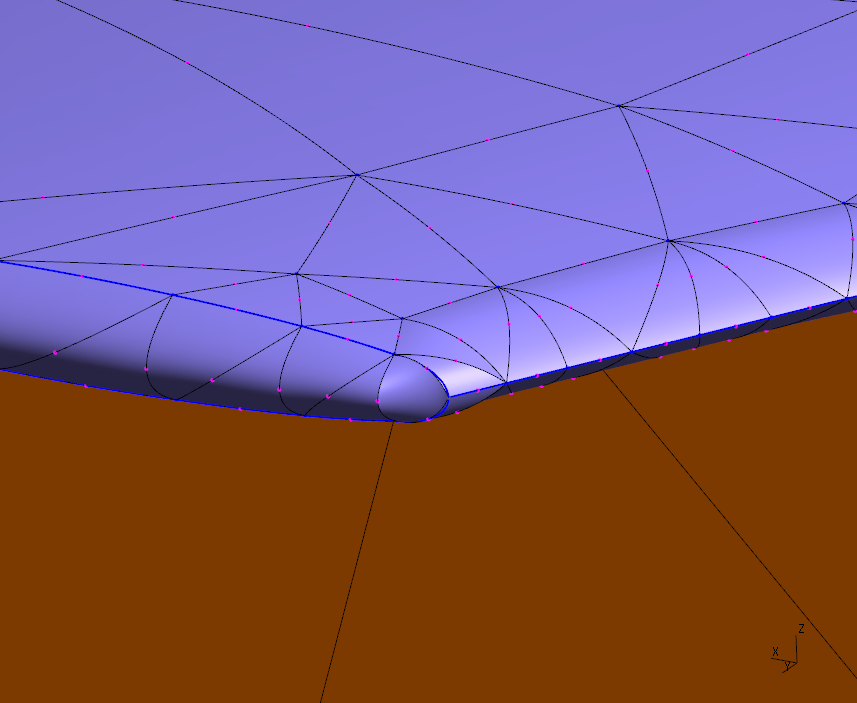
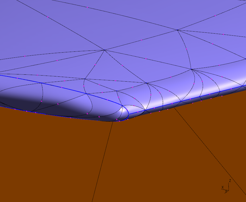
Figure 22: ONERA M6 case: General view of the volume mesh and the wing (top), details of the wing surface mesh optimized for validity only (center left and bottom left) and for both validity and geometrical accuracy (center right and bottom right).

6 Conclusions

In this paper, we have presented methods to evaluate and improve the geometrical representation of CAD models in high-order meshes.

The interest of formal distances in the plane for this purpose has been assessed. The Fréchet and the Hausdorff distances between two curves corresponding respectively to the model and to the mesh boundary have been examined. A discrete version of these quantities, in particular the Hausdorff distance, can be computed fast enough to assess the quality of the geometrical model approximation in practical 2D meshes. However, it is still computationally too costly to be employed in mesh optimization algorithms.

To this end, a fast estimate of the geometrical error between the mesh boundary and the CAD model is presented, which is based on a Taylor development of each curve. It is then introduced in a pre-existing optimization framework that guarantees the mesh validity. Several examples show that minimizing this quantity significantly improves the representation of the model: depending on the case, the model-to-mesh Hausdorff distance is decreased by a factor $2$ to $35$, the gain being larger for coarse meshes. An important aspect of the method lies in the beneficial impact of the geometrical optimization on the mesh boundary smoothness. As evidenced by several test cases, this effect is often instrumental in obtaining accurate solutions from high-order simulations. The approach is easily extended to 3D meshes, as illustrated by two examples.

The method presented in this paper reduces the need to refine a high-order mesh only for the purpose of representing the geometrical model correctly. Therefore, it makes it easier to enjoy the computational efficiency of very high order numerical schemes in practical simulations. However, the constraints of element validity and geometrical accuracy imposed on the mesh may lead to highly curved elements inside the computational domain. The impact of the element distortion on the accuracy, computational cost and robustness of the simulation remains to be assessed and, if possible, controlled. This topic is the subject of ongoing work.

References

- [1] R. Abgrall, C. Dobrzynski, and A. Froehly. A method for computing curved 2D and 3D meshes via the linear elasticity analogy: preliminary results. Rapport de recherche RR-8061, INRIA, Sept. 2012.
- [2] H. Alt and M. Godau. Computing the Fréchet distance between two polygonal curves. International Journal of Computational Geometry & Applications, 5(01n02):75–91, 1995.
- [3] S. Arya, D. M. Mount, N. S. Netanyahu, R. Silverman, and A. Y. Wu. An optimal algorithm for approximate nearest neighbor searching fixed dimensions. Journal of the ACM (JACM), 45(6):891–923, 1998.
- [4] F. Bassi and S. Rebay. High-order accurate discontinuous finite element solution of the 2D Euler equations. J. Comput. Phys., 138(2):251–285, 1997.
- [5] P.-E. Bernard, J.-F. Remacle, and V. Legat. Boundary discretization for high-order discontinuous Galerkin computations of tidal flows around shallow water islands. International Journal for Numerical Methods in Fluids, 59(5):535–557, 2009.
- [6] L. Botti. Influence of reference-to-physical frame mappings on approximation properties of discontinuous piecewise polynomial spaces. Journal of Scientific Computing, 52(3):675–703, 2012.
- [7] B. Cockburn, G. Karniadakis, and C.-W. Shu, editors. Discontinuous Galerkin Methods, volume 11 of Lecture Notes in Computational Science and Engineering, Berlin, 2000. Springer.
- [8] S. Dey, R. M. O’Bara, and M. S. Shephard. Curvilinear mesh generation in 3D. In Proceedings of the 8th International Meshing Roundtable, pages 407–417. John Wiley & Sons, 1999.
- [9] T. Eiter and H. Mannila. Computing discrete Fréchet distance. Technical report, Technische Universitat Wien, 1994.
- [10] A. Gargallo-Peiró, X. Roca, J. Peraire, and J. Sarrate. High-order mesh generation on CAD geometries. In J. P. M. de Almeida, P. Díez, C. Tiago, and N. Parés, editors, Proceedings of the VI International Conference on Adaptive Modeling and Simulation (ADMOS 2013). International Center for Numerical Methods in Engineering (CIMNE), Barcelona, Spain, 2013.
- [11] M. Held. Vroni: An engineering approach to the reliable and efficient computation of Voronoi diagrams of points and line segments. Computational Geometry, 18(2):95–123, 2001.
- [12] A. Johnen, J.-F. Remacle, and C. Geuzaine. Geometrical validity of curvilinear finite elements. In W. R. Quadros, editor, Proceedings of the 20th International Meshing Roundtable, pages 255–271. Springer Berlin Heidelberg, 2012.
- [13] A. Johnen, J.-F. Remacle, and C. Geuzaine. Geometrical validity of curvilinear finite elements. Journal of Computational Physics, 233:359–372, 2013.
- [14] N. Kroll, H. Bieler, H. Deconinck, V. Couaillier, H. Van Der Ven, and K. Sorensen. ADIGMA – A European Initiative on the Development of Adaptive Higher-Order Variational Methods for Aerospace Applications: Results of a Collaborative Research Project Funded by the European Union, 2006-2009. Notes on Numerical Fluid Mechanics and Multidisciplinary Design. Springer, 2010.
- [15] N. Kroll, C. Hirsch, F. Bassi, C. Johnston, and K. Hillewaert, editors. IDIHOM: Industrialization of High-Order Methods - A Top-Down Approach, volume 128 of Notes on Numerical Fluid Mechanics and Multidisciplinary Design. Springer International Publishing, 2015.
- [16] X. Luo, M. Shephard, R. O’Bara, R. Nastasia, and M. Beall. Automatic p-version mesh generation for curved domains. Engineering with Computers, 20(3):273–285, 2004.
- [17] D. Moxey, M. Green, S. Sherwin, and J. Peiró. An isoparametric approach to high-order curvilinear boundary-layer meshing. Computer Methods in Applied Mechanics and Engineering, 283:636–650, 2015.
- [18] P.-O. Persson and J. Peraire. Curved mesh generation and mesh refinement using lagrangian solid mechanics. In Proceedings of the 47th AIAA Aerospace Sciences Meeting and Exhibit, Orlando (FL), USA, 5-9 January 2009, 2009.
- [19] G. Rote. Computing the minimum hausdorff distance between two point sets on a line under translation. Information Processing Letters, 38(3):123–127, 1991.
- [20] O. Sahni, X. Luo, K. Jansen, and M. Shephard. Curved boundary layer meshing for adaptive viscous flow simulations. Finite Elements in Analysis and Design, 46(1-2):132–139, 2010.
- [21] S. J. Sherwin and J. Peiró. Mesh generation in curvilinear domains using high-order elements. International Journal for Numerical Methods in Engineering, 53(1):207–223, 2002.
- [22] T. Toulorge and W. Desmet. Curved boundary treatments for the discontinuous Galerkin method applied to aeroacoustic propagation. AIAA J., 48(2):479–489, 2010.
- [23] T. Toulorge and W. Desmet. Spectral properties of discontinuous Galerkin space operators on curved meshes. In J. S. Hesthaven, E. M. Ronquist, T. J. Barth, M. Griebel, D. E. Keyes, R. M. Nieminen, D. Roose, and T. Schlick, editors, Spectral and High Order Methods for Partial Differential Equations, volume 76 of Lecture Notes in Computational Science and Engineering, pages 495–502. Springer Berlin Heidelberg, 2011.
- [24] T. Toulorge, C. Geuzaine, J.-F. Remacle, and J. Lambrechts. Robust untangling of curvilinear meshes. J. Comput. Phys., 254:8–26, 2013.
- [25] E. Wolanski. Physical Oceanographic Processes of the Great Barrier Reef. CRC Press, Boca Raton, Florida, 1994.
- [26] Z. Q. Xie, R. Sevilla, O. Hassan, and K. Morgan. The generation of arbitrary order curved meshes for 3D finite element analysis. Computational Mechanics, 51(3):361–374, 2013.