Feature Normalisation for Robust Speech Recognition

Abstract.

Speech recognition system performance degrades in noisy environments. If the acoustic models (HMMs) for speech are built using features of clean utterances, the features of a noisy test utterance would be acoustically mismatched with the trained model. This gives poor likelihood values and poor recognition accuracy. Model adaptation and feature normalisation are two broad areas that address this problem. While the former often gives better performance, the latter involves estimation of lesser number of parameters, making the system feasible for practical implementations.

This research focuses on the efficacies of various subspace, statistical and stereo based feature normalisation techniques. A subspace projection based method has been investigated as a standalone and adjunct technique involving reconstruction of noisy speech features from a precomputed set of clean speech building-blocks. The building blocks are learned using non-negative matrix factorisation (NMF) on log-Mel filter bank coefficients, which form a basis for the clean speech subspace. The work provides a detailed study on how the method can be incorporated into the extraction process of Mel-frequency cepstral coefficients. Experimental results show that the new features are more robust to noise, and achieve better results when combined with the existing techniques.

The work also proposes a modification to the training process of the popular SPLICE algorithm for noise robust speech recognition. The modification is based on feature correlations, and enables this stereo-based algorithm to improve the performance in all noise conditions, especially in unseen cases. Further, the modified framework is extended to work for non-stereo datasets where clean and noisy training utterances, but not stereo counterparts, are required. An MLLR-based computationally efficient run-time noise adaptation method in SPLICE framework has been proposed.

Abbreviations and Notations

• Automatic Speech Recognition

• Cepstral Mean Subtraction

• Cepstral Mean and Variance Normalisation

• Gaussian Mixture Model

• Histogram Equalisation

• Heteroscedastic Linear Discriminant Analysis

• Hidden Markov Model

• Interactive voice response

• Log-Mel Filterbank

• Mel-Frequency Cepstral Coefficient

• Maximum Likelihood Linear Regression

• Non-Negative Matrix Factorisation

• Principal Component Analysis

• Stereo-Based Piecewise Linear Compensation for Environments

• Vector Quantisation

• Mean vector

• Covariance matrix

• Divergence function

• HLDA matrix

• Likelihood function

• Positive quadrant of the $D-$dimensional real number space

• (Normal caps font) Constant

• (Normal small font) Variable to the corresponding normal caps font notation

• (Bold caps font) Matrix

• (Bold small font) Vector

• Set of vectors $\mathbf{x}_{1},\mathbf{x}_{2},\ldots,\mathbf{x}_{N}$

• Hadamard (element-wise) matrix product

• Element of the $d^{th}$ row, $n^{th}$ column of the matrix

Chapter 1 Introduction

There are numerous applications of automatic speech recognition (ASR) in the present-day world. From personal mobile assistant apps for the urban population to providing commodity price helplines for farmers in rural areas, speech recognition has made its way from the research laboratories to the common man. More important are the real-time interactive voice response (IVR) based applications for information retrieval and storage, such as automated primary health care, personalised farming, price retrieval, ticket booking and so on.

Such applications, developed on low-end processors, require instant speech-to-text conversion robustly under varying background noises and microphone distortions. Numerous techniques have been proposed to improve the noise robustness of speech recognition. These improved accuracies come at the cost of higher computational complexity. The use of low-end processors limit the processing capability, and also consume time to perform intense computational tasks. This delays the response of the system to the user, making it annoying and often unusable. Thus only a few set of the techniques are suitable for robust real-time ASR systems, and there is an interest in understanding and improving them.

Typical back-end of an ASR system consists of a set of generative hidden Markov models (HMMs) which are trained for each sound unit. Features extracted from the user’s speech data are compared against the HMMs using a process called Viterbi decoding to get the most likely word sequence that could have been spoken. To overcome the effect of noise and distortion, a class of techniques normalise the features of test speech so that they have similar characteristics to those of training.

This thesis concentrates on these feature normalisation techniques suitable for improving robustness in real-time applications. Work has been done on two scenarios, during the training process of the back-end of the system, viz.,

1. there is no information about noise

2. some noisy training speech data are available

1.1. Motivation

Examples of feature normalisation techniques are cepstral mean and variance normalisation (CMVN), histogram equalisation (HEQ), stereo-based piecewise linear compensation for environments (SPLICE) etc. While some of the techniques operate at utterance level and estimate statistical parameters out of the test utterances, some operate on individual feature vectors. Parameter estimation in the former set of techniques requires sufficiently long utterances for reliable estimation, and also some processing. The latter are best suited for shorter utterances and real-time applications.

The standard features used for speech feature extraction are the Mel-frequency cepstral coefficients (MFCCs). In the final stage of their extraction process, a discrete cosine transform (DCT) is used for dimensionality reduction and feature decorrelation. An interesting question to ponder at this juncture is: whether DCT is the best method to achieve feature dimentionality reduction and feature decorrelation along with noise robustness.

Heteroscedastic linear discriminant analysis (HLDA) [Kumar, 1997] is one technique which achieves these qualities under low noise conditions, even though it was originally designed for a different objective. The technique fails in high noise environments. This thesis proposes using non-negative matrix factorisation (NMF) [Lee and Seung, 1999] and reconstruction of the features prior to applying the DCT in the standard MFCC extraction process. Two methods of achieving noise robust features are discussed in detail. These techniques do not assume any information about noise during the training process.

It is also reasonable to identify the commonly encountered noise environments during training, and learn their respective compensations. During the real-time operation of the system, the background noise can be classified into one of the known kinds of noise so that the corresponding compensation can be applied. An example of one such technique is the stereo-based piecewise compensation for environments (SPLICE) [Deng et al., 2000]. This technique requires stereo data during training, which consists of simultaneously recorded speech using two microphones. One is a close-talk microphone capturing mostly clean speech and the other is a far-field microphone, which captures noise along with speech.

This technique is of particular interest because it operates on individual feature vectors, and the compensation is an easily implementable linear transformation of the feature. However, there are two disadvantages of SPLICE. The algorithm fails when the test noise condition is not seen during training. Also, owing to its requirement of stereo data for training, the usage of the technique is quite restricted. This thesis proposes a modified version of SPLICE that improves its performance in all noise conditions, predominantly during severe noise mismatch. An extension of this modification is also proposed for datasets that are not stereo recorded, with minimal performance degradation as compared to the conventional SPLICE. To further boost the performance, run-time adaptation of the parameters is proposed, which is computationally very efficient when compared to maximum likelihood linear regression (MLLR), a standard model adaptation method.

1.2. Overview of the Thesis

The rest of the thesis is organised as follows. Chapter 2 summarises the required background and revises some existing techniques in literature. Chapter 3 discusses the proposed methods of performing feature compensation using NMF during MFCC extraction, and assumes no information about noise during training. Chapter 4 details the proposed modifications and techniques using SPLICE. Finally, Chapter 5 concludes the thesis, indicating possible future extensions.

Chapter 2 Background

2.1. HMM-GMM based Speech Recognition

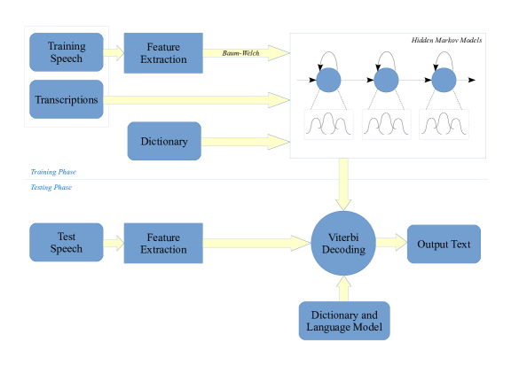
The aim of a speech recognition system is to efficiently convert a speech signal into a text transcription of spoken words [Rabiner and Schafer, 2010]. This requires extracting relevant features from the largely available speech samples, which is called feature extraction. By this process, the speech signal is converted into a stream of feature vectors capturing its time-varying spectral behaviour.

The feature vector streams of each basic sound unit are statistically modelled as HMMs using a training process called Baum-Welch algorithm. This requires sufficient amount of transcribed training speech. A dictionary specifying the conversion of words into the basic sound units is necessary in this process. During testing, an identical feature extraction process, followed by Viterbi decoding are performed to obtain the text output. The decoding is performed on a recognition network built using the HMMs, dictionary and a language model. Language model gives probabilities to sequences of words, and helps in boosting the performance of the ASR system.

This process is summarised in Figure 2.1.1. More detailed explanation can be found in [Rabiner and Schafer, 2010]. The choice of the basic sound unit depends on the size of the vocabulary. Word models are convenient to use for tasks such as digit recognition. For large vocabulary continuous ASR, triphone models are built, which can be concatenated appropriately during Viterbi decoding to represent words.

Figure 2.1.1. Overview of speech recognition system

2.2. MFCC Feature Extraction

Apart from the information about what has been spoken, a speech signal also contains distinct characteristics which vary with the recording conditions such as background noise, microphone distortion, reverberation and so on. Speaker dependent parameters such as vocal tract structure, accent, mood and style of speaking also affect the signal. Thus an ASR system requires robust feature extraction process which captures only the speech information, discarding the rest.

2.2.1. MFCCs

MFCCs have been shown to be one of the effective features for ASR. The extraction of MFCCs is summarised in Figure 2.2.1, and involves the following steps:

1. Short-time processing: Convert the speech signal into overlapping frames. On each frame, apply pre-emphasis to give weightage to higher formants, apply a hamming window to minimise the signal truncation effects, and take magnitude of the DFT.

2. Log Mel filterbank (LMFB): Apply a triangular filterbank with Mel-warping and obtain a single coefficient output for each filter. Apply log operation on each coefficient to reduce the dynamic range. These operations are motivated by the acoustics of human hearing.

3. DCT: Apply DCT on each frame of LMFB coefficients. This provides energy compaction useful for dimensionality reduction, as well as approximate decorrelation useful for diagonal covariance modelling.

   

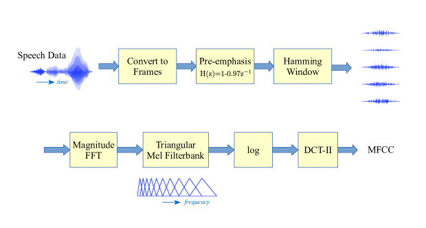
   Figure 2.2.1. Extraction process of MFCCs

A cepstral lifter is generally used to give approximate equal weightage to all the coefficients in MFCCs (the amplitude diminishes due to energy compaction property of DCT). Delta and acceleration coefficients are also appended to the liftered MFCCs, to capture the dynamic information in the speech signal. Finally cepstral mean subtraction (CMS) is performed on these composite features, to remove any stationary mismatch effects caused by recording in different environments.

2.3. Need for Additional Processing

Let us look at the robustness aspects of MFCC composite features in response to two kinds of undesired variations, viz., speaker-based and environment-based.

During MFCC extraction, most of the pitch information is discarded by the smoothing operation of LMFB. Some speaker-specific characteristics are removed by truncating the higher cepstral coefficients after DCT operation. However, other variations such as those occurring due to differences in vocal-tract structures can be compensated for better recognition results.

MFCC composite features are less robust to environment changes. The presence of background noise, especially during testing, causes serious non-linear distortions which cannot be compensated using CMS. This acoustic mismatch between the training and testing environments needs additional compensation.

2.3.1. Feature Compensation and Model Adaptation

The techniques which operate on features to nullify the undesired effects are called feature compensation techniques. Examples are CMVN, HEQ. These methods are usually simple and can be incorporated into real-time applications. So there is an interest in understanding and improving these techniques.

On the contrary, there are a class of model adaptation techniques which refine the models to compensate the effects. These are usually computationally intense and yield high recognition rates. Examples are maximum likelihood linear regression (MLLR), speaker adaptive training (SAT).

Some techniques such as joint factor analysis (JFA), joint uncertainty decoding (JUD) use a combination of both feature and model compensation to further improve the recognition.

However, this thesis focuses on feature compensation done on frame-by-frame basis, due to their suitability to real-time applications.

2.4. A Brief Review of Some Techniques Used

2.4.1. HLDA

Given features belonging to various classes, this technique aims at achieving discrimination among the classes through dimensionality reduction. It linearly transforms $D$ dimensional features such that only $R\;\left(<D\right)$ dimensions of the transformed features have the discriminating capability, and the remaining $D-R$ dimensions can be discarded. In ASR, the features assigned to each state of an HMM during training are typically considered as belonging to a class. The transformation $\boldsymbol{\mathbf{\mathbf{\mathcal{H}}}}$ is estimated from the training data using class labels obtained from their first-pass transcriptions. The $R$ dimensional new features are then used to train and test the models.

Estimation of HLDA transform

Let the feature $\mathbf{y}$ be transformed to obtain $\mathbf{x}=\boldsymbol{\mathbf{\mathbf{\mathcal{H}}}}\mathbf{y}$. Let $\mathbf{y}^{(k)}$ denote that the class-label of $\mathbf{y}$ is $k$. For each class $k$, the set $\left\{\mathbf{y}^{(k)}\right\}$ are assumed to be Gaussian, and thus are their corresponding $\left\{\mathbf{x}^{(k)}\right\}$. It is desired that the last $D-R$ dimensions of $\mathbf{x}$ do not contain any discriminative information, i.e., the mean $\boldsymbol{\mu}_{k}$ and covariance $\boldsymbol{\Sigma}_{k}$ of all the $K$ classes are identical in their last $D-R$ dimensions, as

$$\boldsymbol{\mu}_{k}=\begin{bmatrix}\widetilde{\boldsymbol{\mu}}_{k}\\ \boldsymbol{\mu}_{0}\end{bmatrix},\quad\boldsymbol{\Sigma}_{k}=\begin{bmatrix}\widetilde{\boldsymbol{\Sigma}}_{k}&\mathbf{0}\\ \mathbf{0}&\boldsymbol{\Sigma}_{0}\end{bmatrix}$$

where $\boldsymbol{\mu}_{0}$ and $\boldsymbol{\Sigma}_{0}$ are of dimensions $\left(D-R\right)\times 1$ and $\left(D-R\right)\times\left(D-R\right)$ respectively. If this is achieved, the last $D-R$ dimensions of $\mathbf{x}^{(k)}$ can be discarded without loss of discriminability.

The density of each $\mathbf{y}^{(k)}$ is modelled as

$$p(\mathbf{y}^{(k)})=\frac{|\boldsymbol{\mathbf{\mathcal{H}}}|}{(2\pi)^{\frac{D}{2}}|\boldsymbol{\Sigma}_{k}|^{\frac{1}{2}}}e^{-\frac{1}{2}(\mathbf{x}^{(k)}-\boldsymbol{\mu}_{k})^{T}\boldsymbol{\Sigma}_{k}^{-1}(\mathbf{x}^{(k)}-\boldsymbol{\mu}_{k})}$$

Numerical solution for $\boldsymbol{\mathbf{\mathcal{H}}}$ can be derived by differentiating the log-likelihood function $\mathcal{L}=\sum_{k=1}^{K}\log p(\mathbf{y}^{(k)})$ w.r.t $\boldsymbol{\mathbf{\mathcal{H}}}$, and using the maximum likelihood estimates of $\boldsymbol{\mu}_{k}$ and $\boldsymbol{\Sigma}_{k}$ obtained from $\mathcal{L}$ [Kumar, 1997].

2.4.2. HEQ

HEQ techniques are used to compensate for the acoustic mismatch between the training and testing conditions of an ASR system, thereby giving improved performance. HEQ is a feature compensation technique which defines a transformation that maps the distribution of test speech features onto a reference distribution. As shown in Figure 2.4.1, a function $x=g\left(y\right)$ can be learned such that any noise feature component $y_{0}$ can be transformed to its corresponding equalised version $x_{0}$.

Figure 2.4.1. Illustration of histogram equalisation

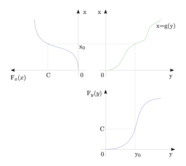
The reference distribution can be that of either clean speech, training data or even a parametric function. Both the training and test features need to be equalised to avoid mismatch. Since HEQ matches the whole distribution, it matches the means, variances and all other higher moments.

Let $y$ be a component of a noisy speech feature vector modelled as $f_{Test}\left(y\right)$. The relation between the cumulative distribution of $y$ and that of its equalised version $x$ is given by

$$F_{Test}\left(y\right) =\int_{-\infty}^{y}f_{Test}\left(y^{\prime}\right)dy^{\prime}$$

$$=\int_{-\infty}^{g\left(y\right)}f_{Test}\left(g^{-1}\left(x^{\prime}\right)\right)\frac{dg^{-1}\left(x^{\prime}\right)}{dx^{\prime}}dx^{\prime}$$

$$=\int_{-\infty}^{x}f_{Train}\left(x^{\prime}\right)dx^{\prime}\;\bigg{|}_{x=g\left(y\right)}$$

$$=F_{Train}\left(x\right)$$

In practice, the function $g\left(y\right)$ is implemented using quantile-based methods [Hilger and Ney, 2006].

2.4.3. MLLR

MLLR is a widely used adaptation technique based on maximum-likelihood principle [Legetter, 1995, Gales, 1998]. It performs adaptation through regression-based transformations on (usually) the mean vectors $\boldsymbol{\mu}_{m}$ of the system of HMMs, $m$ being the mixture index. The transformations are estimated such that the original system is tuned to a new speaker or environment.

$$\widetilde{\boldsymbol{\mu}}_{m}=\mathbf{\boldsymbol{\mathcal{M}}}_{m}\boldsymbol{\mu}^{\prime}_{m}$$

where $\mathbf{\boldsymbol{\mathcal{M}}}_{m}$ is an MLLR transformation matrix of dimension $D\times\left(D+1\right)$, and $\boldsymbol{\mu}^{\prime}_{m}=\begin{bmatrix}1&\boldsymbol{\mu}_{m}^{T}\end{bmatrix}^{T}$. An estimate of $\boldsymbol{\mathbf{\mathcal{M}}}_{m}$ is obtained by maximising the likelihood function

$$\mathbf{\mathcal{L}}=\frac{1}{(2\pi)^{\frac{D}{2}}|\boldsymbol{\Sigma}_{m}|^{\frac{1}{2}}}e^{-\frac{1}{2}(\mathbf{x}-\mathbf{\mathbf{\boldsymbol{\mathcal{M}}}_{m}}\boldsymbol{\mu}^{\prime}_{m})^{T}\boldsymbol{\Sigma}_{m}^{-1}(\mathbf{x}-\mathbf{\boldsymbol{\mathcal{M}}}_{m}\boldsymbol{\mu}^{\prime}_{m})}$$

In this work, MLLR mean adaptation has been used as a global transform to adjust the system of HMMs to a new noise environment encountered during testing. The adaptation data are the same as test data, which consist of files recorded in a particular noise condition with sufficient speaker and speech variations.

2.4.4. SPLICE

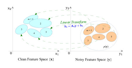
SPLICE is a popular and efficient noise robust feature enhancement technique. It partitions the noisy feature space into $M$ classes, and learns a linear transformation based noise compensation for each partition class during training, using stereo data. Any test vector $\mathbf{y}$ is soft-assigned to one or more classes by computing $p\left(m\,|\,\mathbf{y}\right)$ $\left(m=1,2,\ldots,M\right)$, and is compensated by applying the weighted combination of linear transformations to get the cleaned version $\widehat{\mathbf{x}}$.

(2.4.1) $$\widehat{\mathbf{x}}=\sum_{m=1}^{M}p\left(m\,|\,\mathbf{y}\right)\left(\mathbf{A}_{m}\mathbf{y}+\mathbf{b}_{m}\right)$$

$\mathbf{A}_{m}$ and $\mathbf{b}_{m}$ are estimated during training using stereo data. The training noisy vectors $\{\mathbf{y}\}$ are modelled using a Gaussian mixture model (GMM) $p(\mathbf{y})$ of $M$ mixtures, and $p\left(m\,|\,\mathbf{y}\right)$ is calculated for a test vector as a set of posterior probabilities w.r.t the GMM $p(\mathbf{y})$. Thus the partition class is decided by the mixture assignments $p\left(m\,|\,\mathbf{y}\right)$. This is illustrated in Figure 2.4.2.

Figure 2.4.2. Illustration of SPLICE feature enhancement

2.4.5. NMF

NMF is an approximate matrix decomposition

(2.4.2) $$\underset{\left(D\times N\right)}{\mathbf{V}}\approx\underset{\left(D\times R\right)}{\mathbf{W}}\underset{\left(R\times N\right)}{\mathbf{H}}$$

where $\mathbf{V}$, consisting of non-negative elements, is decomposed into two non-negative matrices $\mathbf{W}$ and $\mathbf{H}$. In the context of speech data, the columns of $\mathbf{V}$ constitute non-negative feature vectors $\{\mathbf{v}_{n}\}\in\mathbb{R}^{D+},\,n=1,2,\ldots,N$. After the decomposition, $\mathbf{W}$ is a non-negative dictionary of basis vectors $\{\mathbf{w}_{r}\}\in\mathbb{R}^{D+},\,r=1,2,\ldots,R$ along columns, representing a useful subspace in which $\{\mathbf{v}_{n}\}$ are contained, when $R<D$. $\mathbf{H}\in\mathbb{R}^{(R\times N)+}$ is a matrix of vectors $\{\mathbf{h}_{n}\}\in\mathbb{R}^{R+},n=1,2,\ldots,N$ such that each $\mathbf{h}_{n}=\{h_{1n},h_{2n},\ldots,h_{Rn}\}$ is a set of weights or activation coefficients acting upon all the bases $\{\mathbf{w}_{r}\}$ to give the corresponding $\mathbf{v}_{n}$, independently of all the other columns, as shown in equation 2.4.3.

(2.4.3) $$\mathbf{v}_{n}\approx\sum_{r=1}^{R}\mathbf{w}_{r}h_{rn}$$

The decomposition (2.4.2) can be learned by randomly initialising $\mathbf{W}$ and $\mathbf{H}$. The estimates of $\mathbf{W}$ and $\mathbf{H}$ are iteratively improved by minimising a KL-divergence based cost function

(2.4.4) $$\mathcal{D}(\mathbf{V}\parallel\mathbf{WH})=\sum_{d,n}\left[\mathbf{V}\otimes\log\left(\frac{\mathbf{V}}{\mathbf{W}\mathbf{H}}\right)-\mathbf{V}+\mathbf{WH}\right]_{dn}$$

where $\otimes$ denotes Hadamard product, the division inside the log is element-wise and the summation is over all the elements of the matrix. The optimisation

$$\underset{\mathbf{W},\mathbf{H}}{\arg\min}\enskip\mathcal{D}(\mathbf{V}\parallel\mathbf{WH})\qquad\mathbf{W}>0,\enskip\mathbf{H}>0$$

gives the following iterative update rules [Lee and Seung, 1999, Lee and Seung, 2000] for refining the matrices $\mathbf{W}$ and $\mathbf{H}$:

(2.4.5) $$w_{dr}:=w_{dr}\frac{\sum_{n}h_{rn}v_{dn}/[\mathbf{WH}]_{dn}}{\sum_{n}h_{rn}}$$

(2.4.6) $$h_{rn}:=h_{rn}\frac{\sum_{d}w_{dr}v_{dn}/[\mathbf{WH}]_{dn}}{\sum_{d}w_{dr}}$$

where “$:=$” refers to assignment operator. It can be seen that the update rules are multiplicative, i.e., the matrices are updated by performing just a product with another matrix, making the implementation simple and quick. The columns of $\mathbf{W}$ can be thought of as basic building blocks that can reconstruct speech features.

2.5. Recent Work in Literature - Motivation

[Sainath et al., 2012] showed an overview of a wide range of techniques in ASR that use speech exemplars (dictionaries). It was argued that noise robustness can be achieved through the use of speech dictionaries. However, most of these techniques are computationally intense.

Since NMF is one of the methods of learning dictionaries and is easily implementable, it is of particular interest. NMF is known to learn useful time-frequency patterns in a given dataset, and has been applied to learn spectral representations in audio and speech applications that include audio source separation, supervised speech separation, speech enhancement and recognition. A few of them are mentioned below.

A regularised variant of NMF was used by [Wilson et al., 2008] to learn separate dictionaries of speech and noise. The concatenated dictionary was used in NMF to learn weights of noisy test utterances, where the weights corresponding to noise bases are suppressed to achieve speech denoising and thus enhancement. [Schuller et al., 2010] proposed supervised NMF for improving noise robustness in spelling recognition task. NMF was performed using a predetermined $\mathbf{W}$ consisting of spectra of spelled letters. The authors showed that appending the weights $\mathbf{H}$ to MFCC and BLSTM (Bidirectional Long Short-Term Memory neural network) features improves noise robustness. [Gemmeke et al., 2011] represented LMFB features of noisy speech using exemplars of speech and noise bases. A hybrid (exemplar and HMM based) recognition on Aurora-2 task was performed to achieve noise robustness at high noise levels.

Most of the above techniques have used the weights $\mathbf{H}$ as new features or combining them with existing features for improved recognition. In contrast, Chapter 3 of this thesis will show that multiplying back $\mathbf{W}$ and $\mathbf{H}$ to get new LMFB features and converting them to MFCCs improves noise robustness. This approach is useful in real-time applications because of its fast implementation. A technique which learns a robust $\mathbf{W}$ will also be discussed. These methods do not assume any information about noise during training.

When there are noisy training files available, techniques such as SPLICE learn compensation from the seen noisy data to obtain their corresponding clean versions. Over the last decade, improvements using uncertainty decoding [Droppo et al., 2002], maximum mutual information based training [Droppo and Acero, 2005], speaker normalisation [Shinohara et al., 2008] etc. were introduced in SPLICE framework. There are two disadvantages of SPLICE. The algorithm fails when the test noise condition is not seen during training. Also, owing to its requirement of stereo data for training, the usage of the technique is quite restricted. So there is an interest in addressing these issues.

[Chijiiwa et al., 2012] recently proposed an adaptation framework using Eigen-SPLICE to address the problem of unseen noise conditions. The method involves preparation of quasi stereo data using the noise frames extracted from non-speech portions of the test utterances. For this, the recognition system is required to have access to some clean training utterances for performing run-time adaptation.

[Gonzalez et al., 2011] proposed a stereo-based feature compensation method, which is similar to SPLICE in certain aspects. Clean and noisy feature spaces were partitioned into vector quantised (VQ) regions. The stereo vector pairs belonging to $i^{th}$ VQ region in clean space and $j^{th}$ VQ region in noisy space are classified to the $ij^{th}$ sub-region. Transformations based on Gaussian whitening expression were estimated from every noisy sub-region to clean sub-region. But it is not always guaranteed to have enough data to estimate a full transformation matrix from each sub-region to other.

In Chapter 4, a simple modification to SPLICE will be proposed, based on an assumption made on the correlation of training stereo data. This will be shown to give improved performance in all the noise conditions, predominantly in unseen conditions which are highly mismatched with those of training. An extension of the method to non-stereo datasets (which are not stereo recorded) will be proposed, with minimal performance degradation as compared to conventional SPLICE. Finally, an MLLR-based run-time noise adaptation framework will be proposed, which is computationally efficient and achieves better results than MLLR-based model adaptation.

Chapter 3 Non-Negative Subspace Projection

3.1. Introduction

During MFCC extraction, usually 23 LMFB coefficients are converted into 13 dimensional MFCCs through DCT. Results in Table 3.1 show that performing HLDA on 39 dimensional MFCCs gives better robustness to noise than MFCCs when the noise levels are low. But this technique fails in high noise conditions. However, the objective of HLDA is not to achieve robustness, but class-separability. Here a method is proposed which aims at finding representations of speech feature vectors using building-blocks.

Figure 3.1.1. NMF subspace projection

The method operates on LMFB feature vectors by representing them using non-negative linear combinations of their non-negative building blocks. DCT-II is applied on the new feature vectors to obtain new MFCCs. This incorporates, into the MFCC extraction process, a concept that the speech features are made up of underlying building blocks. Apart from the proposed additional step, conventional MFCC extraction framework is maintained throughout the process. The building blocks of speech are learned using NMF on speech feature vectors. Experimental results show that the new MFCC features are more robust to noise, and achieve better results when combined with the existing noise robust feature normalisation techniques like HEQ and HLDA.

3.2. The Speech Subspace

The columns of $\mathbf{W}$ can be thought of as basic building blocks that construct all the speech feature vectors, or the bases for subspace of the speech feature vectors. So far, no mathematical proof has been derived to validate if NMF learns the representations of the underlying data. However, much of the literature support this. [Smaragdis, 2007] states that the basis functions describe the spectral characteristics of the input signal components, and reveal its vertical structure. [Wilson et al., 2008] refer to these building blocks as a set of spectral shapes. [Schuller et al., 2010] refer to them as spectra of events occurring in the signal, and NMF is known to learn useful time-frequency patterns in a given dataset.

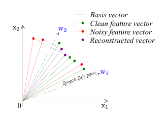
One could probably use other basis learning techniques like principal component analysis (PCA) to estimate the clean subspace. Though PCA finds the directions of maximum spread of the features, these directions need not contain only speech information. In methods such as NMF, new features can be reconstructed within the subspace using different cost functions to achieve desired qualities such as source localisation, sparseness etc. KL-divergence based NMF has been successfully applied in speech applications [Wilson et al., 2008, Schuller et al., 2010] over the conventional Euclidean distance measure. In addition, the non-negativity constraint is an added advantage. Figure 3.1.1 shows the bases $\mathbf{w}_{1}$ and $\mathbf{w}_{2}$ learned by NMF on two-dimensional data contained in the subspace shown. Any vector outside this subspace cannot be reconstructed perfectly using $\mathbf{w}_{1}$ and $\mathbf{w}_{2}$ when the weights acting on them are constrained to be non-negative. So when these features are moved away from the subspace due to the effect of noise, the reconstructed features can be used in place of these features as better representations of the underlying signal. However, vectors still inside the subspace are not compensated.

(a) Original features

(b) Reconstruction using NMF individual basis vectors

Figure 3.2.1. LMFB features of a speech utterance

3.3. Learning the Speech Subspace

NMF can be performed by optimising cost functions based on different measures such as Euclidean, KL-divergence, Itakura-Saito distances. Here KL-divergence based method is chosen, which gives the update equations (2.4.5) and (2.4.6). The decomposition is not unique since the cost function (2.4.4) to be optimised is not convex. Depending on the application, one may choose to perform update on both $\mathbf{W}$ and $\mathbf{H}$ in each iteration, or fix one matrix and update the other. While simultaneously refining $\mathbf{W}$ and $\mathbf{H}$, the columns of $\mathbf{W}$ may be normalised after each update so that the sum of each column adds up to value $1$. The scaling is automatically compensated in weight matrix $\mathbf{H}$ during its update.

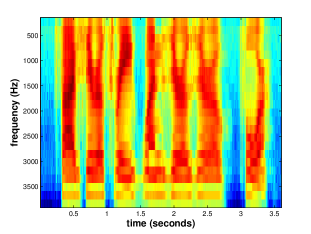
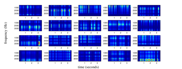
Fig. 3.2.1a shows the plot of LMFB outputs of an utterance containing connected spoken digits. Using the dictionary learned from Aurora-2 database (as described in Section 3.4.1), the reconstructions of the same utterance from each individual basis vector of $\mathbf{W}$ are plotted in Fig. 3.2.1b. It can be observed that each of the reconstructions has only a set of particular dominant frequencies that are captured by the corresponding basis vector. Such a dictionary can capture useful combinations of frequencies present in speech utterances, and can give noise-robust speech reconstructions. The reconstructed feature vectors are more correlated, due to their confinement to the speech subspace, than the original ones.

In PCA method, the speech dictionary $\mathbf{W}$ can be built by stacking the most significant Eigen vectors of the clean training data as columns. Any speech feature $\mathbf{v}$ can be reconstructed as

$$\widehat{\mathbf{v}}=\mathbf{W}\mathbf{W}^{T}\mathbf{v}$$

3.4. Proposed Feature Extraction Methods

Speech signal is passed through conventional short-time processing steps followed by an LMFB. Before applying DCT, which corresponds to obtaining the conventional MFCC features, an additional step is proposed to be introduced as shown in Fig. 3.4.1, so that the new MFCCs obtained after the processing are more robust to noise. The additional step is computed in two different methods as described in Sections 3.4.1 and 3.4.2, and the performances are compared in Sections 4.5.2.

Short-time processing of speech signal includes applying STFT with Hamming window of length 25$ms$ at a frame rate of 100 frames/second, followed by passing the mean subtracted frames through a pre-emphasis filter $1-0.97z^{-1}$. A conventional Mel-filter bank of $23$ constant bandwidth equal gain linear triangular filters on the Mel scale is applied to get a set of filter outputs for each frame. These outputs are Mel-floored to value 1.0, and log operator is applied to obtain non-negative LMFB feature vectors $\{\mathbf{v}_{n}\}$.

Let the LMFB feature vectors $\{\mathbf{v}_{\zeta}\}$ and $\{\mathbf{v}_{\varphi}\}$ corresponding to the training and test speech be stacked as columns of $\mathbf{V}_{\zeta}$ and $\mathbf{V}_{\varphi}$ respectively.

3.4.1. NMF_plain

$\mathbf{V}_{\zeta}$ is decomposed as $\mathbf{V}_{\zeta}\approx\mathbf{W}_{\zeta}\mathbf{H}_{\zeta}$ using NMF decomposition by simultaneously updating $\mathbf{W}_{\zeta}$ and $\mathbf{H}_{\zeta}$ by (2.4.5) and (2.4.6). Each column of $\mathbf{W}_{\zeta}$ is normalised after every iteration. Finally, $\mathbf{W}_{\zeta}$ learns the building blocks of these feature vectors. During testing, $\mathbf{V}_{\varphi}$ is approximated as the product of $\mathbf{W}_{\zeta}$ and $\mathbf{H}_{\varphi}$ (i.e., $\mathbf{V}_{\varphi}\approx\mathbf{W}_{\zeta}\mathbf{H}_{\varphi}$). This is done by fixing $\mathbf{W}_{\zeta}$ obtained during training and performing update on $\mathbf{H}_{\varphi}$ alone using (2.4.6). The new feature vectors in training and testing are thus

(3.4.1) $$\widehat{\mathbf{V}}_{\zeta}=\mathbf{W}_{\zeta}\mathbf{H}_{\zeta}$$

and

(3.4.2) $$\mathbf{\widehat{V}}_{\varphi}=\mathbf{W}_{\zeta}\mathbf{H}_{\varphi}$$

respectively. In the implementation, the whole training data has been taken as $\mathbf{V}_{\zeta}$ to compute $\mathbf{W}_{\zeta}$ using NMF. However, during testing, each test utterance can separately be taken as $\mathbf{V}_{\varphi}$ and the corresponding $\mathbf{H}_{\varphi}$ can be computed, fixing $\mathbf{W}_{\zeta}$.

Figure 3.4.1. Computation of subspace projected MFCCs

Here the assumption is that many of the columns of $\mathbf{V}_{\varphi}$ are initially outside the speech subspace due to the effect of noise. If each of these vectors outside the subspace is mapped to the nearest vectors $\widehat{\mathbf{V}}_{\varphi}$ within the subspace, the new features are more noise-robust. If noise moves a clean feature vector to another vector in the same subspace, it cannot be compensated. Here the subspace is captured by $\mathbf{W}_{\zeta}$, and the term nearest is meant in the measure of KL-divergence distance. Replacement of $\mathbf{V}_{\varphi}$ by $\widehat{\mathbf{V}}_{\varphi}$ can alternatively be justified as follows. Each $\mathbf{v}_{\varphi}$ is being represented by non-negative linear combinations of building blocks $\mathbf{w}_{\zeta}$ of speech data, because of which any noise component in $\mathbf{v}_{\varphi}$ cannot be reconstructed using speech bases, and hence cannot be retained in $\mathbf{\widehat{v}}_{\varphi}$.

Now, by convention, DCT matrix $\mathbf{D}$, followed by a standard cepstral lifter $\mathbf{L}$ are applied on the features $\mathbf{V}_{\zeta}$ and $\mathbf{V}_{\varphi}$ to obtain 13 dimensional MFCC features ($C_{0}\ldots C_{12}$) for each frame, given by Eqs. (3.4.3) and (3.4.4).

(3.4.3) $$\mathbf{C}_{\zeta}=\mathbf{LD}\widehat{\mathbf{V}}_{\zeta}$$

(3.4.4) $$\mathbf{C}_{\varphi}=\mathbf{LD}\widehat{\mathbf{V}}_{\varphi}$$

These features are used to parameterise the acoustic models (HMMs), as explained in Section 3.6.1.

3.4.2. NMF_robustW

Each set of basis activation coefficients $\mathbf{h}_{n}$ (for both training and test data) is unique for the corresponding speech frame. An addition of noise changes the statistics of $\mathbf{h}_{n}$. So it is intuitive that equalising the statistics of $\mathbf{H}_{\varphi}$ during testing, to match that of training $\mathbf{H}_{\zeta}$, improves the recognition. The equalisation has to be applied during training also, to avoid mismatch of the test features against the built acoustic model. Here the intention is not to perform test feature equalisation explicitly, but to get a dictionary $\widetilde{\mathbf{W}}_{\zeta}$ which helps learn the test weights that are in equalised form, and thus are more robust. Figure 3.4.2 shows a method of obtaining the better dictionary $\widetilde{\mathbf{W}}_{\zeta}$ from $\mathbf{W}_{\zeta}$, $\mathbf{H}_{\zeta}$ and $\mathbf{V}_{\zeta}$, using HEQ during training.

Figure 3.4.2. Learning the speech dictionary in NMF_robustW

After decomposing $\mathbf{V}_{\zeta}$ as $\mathbf{V}_{\zeta}\approx\mathbf{W}_{\zeta}\mathbf{H}_{\zeta}$ using NMF, a set of $R$ reference histograms $\left\{Q_{r}\right\}$ of $\mathbf{H}_{\zeta}$ are calculated, one for each of its feature component. HEQ is performed on $\mathbf{H}_{\zeta}$, as described in Section 3.5, to get better or more robust activations $\mathbf{\widetilde{H}}_{\zeta}$. But $\mathbf{W}_{\zeta}\mathbf{\widetilde{H}}_{\zeta}$ no longer matches $\mathbf{V}_{\zeta}$. So a better $\mathbf{W}_{\zeta}$ is estimated using NMF update (2.4.5), i.e., by fixing $\mathbf{\widetilde{H}}_{\zeta}$, $\mathbf{V}_{\zeta}$ and updating $\mathbf{W}$. This essentially solves the optimisation

$$\widetilde{\mathbf{W}}_{\zeta}=\underset{\mathbf{W}}{\arg\min}\enskip D(\mathbf{V_{\zeta}}\parallel\mathbf{W\widetilde{H}_{\zeta}})\qquad\mathbf{W}>0,\enskip\mathbf{\widetilde{H}_{\zeta}}>0$$

In other words, the speech dictionary is chosen such that the weights become statistically equalised during training. Experimental results show that $\widetilde{\mathbf{W}}_{\zeta}$ is a better dictionary than $\mathbf{W}_{\zeta}$ in terms of noise-robustness. The training features are thus

(3.4.5) $$\widehat{\mathbf{V}}_{\zeta}=\mathbf{\widetilde{W}}_{\zeta}\mathbf{\widetilde{H}}_{\zeta}$$

Testing process is the same as described in Section 3.4.1, except that the new $\widetilde{\mathbf{W}}_{\zeta}$ is directly used to estimate the test data weights $\mathbf{H}_{\varphi}$, instead of $\mathbf{W}_{\zeta}$. Additional equalisation is not performed during testing, since the dictionary itself helps in learning equalised weights. The test features are thus

(3.4.6) $$\mathbf{\widehat{V}}_{\varphi}=\mathbf{\widetilde{W}}_{\zeta}\mathbf{H}_{\varphi}$$

As per convention, DCT and cepstral lifter matrices are applied on $\widehat{\mathbf{V}}_{\zeta}$ and $\mathbf{\widehat{V}}_{\varphi}$, given by Eqs. (3.4.3) and (3.4.4) to obtain the 13 dimensional MFCC feature vectors for training and testing the HMMs. Here it can be seen that the computational cost of both NMF_plain and NMF_robustW are the same during testing.

3.5. Cascading with Existing Techniques

The proposed methods can be cascaded with HEQ, where reference histogram can be built using $\mathbf{C}_{\zeta}$, and HEQ can be applied on $\mathbf{C}_{\zeta}$ and $\mathbf{C}_{\varphi}$ to get new features vectors, using which acoustic models can be built as described in Section 3.6.1.

Since the feature vectors given by Eqs. (3.4.1) and (3.4.2) are constrained to the column space of $\mathbf{W}_{\zeta}$, there is certain additional correlation introduced in them. Their corresponding cepstral features $\mathbf{C}_{\zeta}$ and $\mathbf{C}_{\varphi}$ are made approximately decorrelated through the use of DCT. However, an additional decorrelation using HLDA is expected to further reduce the feature correlations, besides utilising the advantage of subspace projection. This also makes them more suitable for diagonal covariance modelling. The HLDA transformation matrix is estimated in maximum likelihood (ML) framework after building the acoustic models using 39 dimensional MFCCs as described in [Kumar and Andreou, 1998], and is applied to both feature vectors and the models in the conventional method.

3.6. Experiments and Results

3.6.1. Experimental Setup

Aurora-2 task [Hirsch and Pearce, 2000] has been used to perform a comparative study of the proposed techniques versus the existing ones. Aurora-2 consists of connected spoken digit utterances of TIDigits database, filtered and resampled to 8 kHz, and with noises added at different SNRs. The noises are sounds recorded in places such as train station, crowd of people, restaurant, interior of car etc. The availability of both clean and noisy versions of the training speech utterances makes them stereo in nature. The test set consists of 10 sets of utterances, each with one noise environment added, and each at seven distinct SNR levels.

The acoustic word models for each digit have been built using left to right continuous density HMMs with 16 states and 3 diagonal covariance Gaussian mixtures per state. For all the experiments, $C_{0}$ included MFCC vectors of 13 dimensions, obtained from the signal processing blocks, are appended with 13 delta and 13 acceleration coefficients to get a composite 39 dimensional vector per frame. Cepstral mean subtraction (CMS) has been performed on these vectors, and the resultant feature vectors are used for building the acoustic models for each digit, which in Aurora-2 task is a left to right continuous density HMM with 16 states and 3 diagonal covariance Gaussian mixtures per state. HMM Toolkit (HTK) 3.4.1 [Young et al., 2009] has been used for building and testing the acoustic models.

NMF has been implemented using MATLAB software. The size of the speech dictionary (in other words, the dimensionality of the speech subspace) has been optimised and chosen as $R=20$ throughout the experiments based on recognition results. It is to be noted that during NMF, LMFB feature vectors are of dimension $D=23$. While performing NMF, $\mathbf{W}$ has been initialised from random columns of $\mathbf{V}$, and $\mathbf{H}$ with random numbers in $[0,1]$. 500 iterations of NMF are performed in all the experiments.

For performing HEQ, quantile based method has been employed, dividing the range of cdf values into 100 quantiles. In the experiments including HLDA, all 39 directions are retained, since the aim is to observe only the performance improvement after nullifying the correlations.

3.6.2. Results

Table 3.1. Subspace projection on Aurora-2 database

Noise Level	Baseline	NMF_plain	NMF_robustW
Clean	99.25	99.27	99.02
SNR 20	97.35	97.50	97.45
SNR 15	93.43	94.17	95.00
SNR 10	80.62	82.73	86.94
SNR 5	51.87	56.48	65.48
SNR 0	24.30	25.97	32.46
SNR -5	12.03	12.46	12.68
Average	69.51	71.37	75.47

(a) Individual methods

Noise Level	HLDA	NMF_plain + HLDA	NMF_robustW + HLDA
Clean	99.35	99.35	99.28
SNR 20	98.11	98.25	98.26
SNR 15	94.84	95.69	96.20
SNR 10	82.08	87.14	89.76
SNR 5	49.85	63.63	70.95
SNR 0	21.64	28.31	35.41
SNR -5	11.15	11.47	12.97
Average	69.30	74.60	78.11

(b) Cascading with HLDA

Noise Level	HEQ	NMF_plain + HEQ	NMF_robustW + HEQ
Clean	99.03	98.94	98.73
SNR 20	97.68	97.76	97.21
SNR 15	95.39	95.93	95.26
SNR 10	90.00	91.49	90.67
SNR 5	75.61	79.21	78.79
SNR 0	46.66	51.63	53.04
SNR -5	18.37	19.54	21.28
Average	81.07	83.20	82.99

(c) Cascading with HEQ

Figure 3.6.1. Results of PCA as a subspace projection step

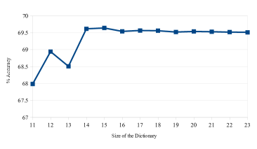
Table 3.1 shows the recognition accuracies of the various techniques on Aurora-2 database. Average values shown are taken over SNR levels $20-0$ dB. Table 3.1a shows the accuracies of proposed methods. Tables 3.1b and 3.1c show how the methods improve when cascaded with HLDA and HEQ respectively. It can be observed that HLDA can be used to achieve noise robustness in low noise levels only, and fails at high noise levels (SNR $5$ to $-5$ dB). In the PCA method as shown in Figure 3.6.1, a dictionary of size $23$ is an orthogonal matrix which retains all the directions, thus corresponding exactly to the baseline system. It can be seen that this method hardly gives an improvement over the baseline at different dictionary sizes. NMF_plain gives $1.86\%$ absolute improvement in recognition accuracy, NMF_plain cascaded with HLDA gives $5.09\%$, NMF_robustW gives $5.96\%$, NMF_robustW+HLDA gives $8.6\%$. NMF_plain+HEQ gives $13.69\%$ and NMF_robustW gives $13.48\%$ improvement.

Specifically at SNR 5 dB, the individual proposed methods NMF_plain and NMF_robustW give absolute improvements by $4.61\%$ and $11.76\%$ respectively. When combined with HEQ, the highest improvement achieved is $27.3\%$ at SNR $5$ and $0$ dB. Figure 3.6.1 shows the accuracy of using PCA as a feature processing step at different sizes of the dictionary.

The combination of NMF_plain+HEQ+HLDA achieved a recognition accuracy of $81.26\%$. This is not a comparable improvement over the other proposed techniques, considering the increased computational complexity.

3.7. Discussion

Methods described in Sections 3.4.1 and 3.4.2 are observed to give improvements in all noise conditions at all SNR levels, and give significantly better performances in moderate to high noise conditions. NMF_robustW+HEQ does not give improvement over NMF_plain+HEQ, both of them perform almost equally well. So when almost equalised weights $\mathbf{H}_{\varphi}$ are obtained through NMF_robustW, there is no advantage when an additional equalisation is done in cepstral domain.

The proposed methods have notable advantages of over other techniques in literature. There is no need of building a separate dictionary for capturing noise characteristics, for which training audio files containing pure noise would have been required. The methods operate on each speech frame independently, and so they can even handle very short utterances, unlike HEQ where the estimate of $F_{test}(x)$ will be poor for short utterances. The methods are seen to give advantage when combined with other feature normalisation techniques. Finally the proposed methods are simple, easy to implement, and are achievable without the use of some commonly used additional tools like speech/silence detector, pre-built CDHMM model etc.

The proposed methods have a few disadvantages. The decomposition is iterative and the step size of the update rules (2.4.5) and (2.4.6) is small. So it takes many iterations to converge, and the number of iterations increases when the size of the database is large. Dictionary estimation from a very large database is computationally expensive and is limited by the availability of memory in the computing device. Iterations have to be performed even during testing, to determine the weights $\mathbf{H_{\varphi}}$.

Thus the concept of building-blocks representation of speech is incorporated into the features, still preserving the advantages of using MFCCs. Conventional HMM based recogniser has been used to test the efficacy of the proposed MFCCs against the standard MFCCs.

Chapter 4 Stereo and Non-Stereo Based Feature Compensation

In this chapter, the techniques based on SPLICE are studied. A simple modification to SPLICE is proposed, based on an assumption made on the correlation of training stereo data. This is shown to give improved performance in all the noise conditions, predominantly in unseen conditions which are highly mismatched with those of training. This method does not need any adaptation data, in contrast to the recent work proposed in literature [Chijiiwa et al., 2012], and has been termed as modified SPLICE (M-SPLICE). M-SPLICE has also been extended to work for datasets that are not stereo recorded, with minimal performance degradation as compared to conventional SPLICE. Finally, an MLLR-based run-time noise adaptation framework has been proposed, which is computationally efficient and achieves better results than MLLR HMM-adaptation. This method is done on 13 dimensional MFCCs and does not require two-pass Viterbi decoding, in contrast to conventional MLLR done on 39 dimensions.

4.1. Review of SPLICE

As discussed in the introduction, SPLICE algorithm makes the following two assumptions:

1. The noisy features $\left\{\mathbf{y}\right\}$ follow a Gaussian mixture density of $M$ modes

   (4.1.1) $$p(\mathbf{y})=\sum_{m=1}^{M}P(m)p(\mathbf{y}\,|\,m)=\sum_{m=1}^{M}\boldsymbol{\pi}_{m}\mathcal{N}\left(\mathbf{y}\,;\,\boldsymbol{\mu}_{y,m},\boldsymbol{\Sigma}_{y,m}\right)$$

2. The conditional density $p(\mathbf{x}\,|\,\mathbf{y},m)$ is the Gaussian

   (4.1.2) $$p(\mathbf{x}\,|\,\mathbf{y},m)\sim\mathcal{N}\left(\mathbf{x}\,;\,\mathbf{A}_{m}\mathbf{y}+\mathbf{b}_{m},\boldsymbol{\Sigma}_{x,m}\right)$$

   where $\{\mathbf{x}\}$ are the clean features.

Thus, $\mathbf{A}_{m}$ and $\mathbf{b}_{m}$ parameterise the mixture specific linear transformations on the noisy vector $\mathbf{y}$. Here $\mathbf{y}$ and $m$ are independent variables, and $\mathbf{x}$ is dependent on them. Estimate of the cleaned feature $\widehat{\mathbf{x}}$ can be obtained in MMSE framework as shown in Eq. (2.4.1).

The derivation of SPLICE transformations is briefly discussed next. Let $\mathbf{W}_{m}=\begin{bmatrix}\mathbf{b}_{m}&\mathbf{A}_{m}\end{bmatrix}$ and $\mathbf{y}^{\prime}=\begin{bmatrix}1&\mathbf{y}^{T}\end{bmatrix}^{T}$. Using $N$ independent pairs of stereo training features $\left\{\left(\mathbf{x}_{n},\mathbf{y}_{n}\right)\right\}$ and maximising the joint log-likelihood

(4.1.3) $$\mathcal{L}=\sum_{n=1}^{N}\log p(\mathbf{x}_{n},\mathbf{y}_{n})=\sum_{n=1}^{N}\log\left[\sum_{m=1}^{M}p(\mathbf{x}_{n}\,|\,\mathbf{y}_{n},m)p(\mathbf{y}_{n}\,|\,m)P(m)\right]$$

yields

(4.1.4) $$\mathbf{W}_{m}=\left[\sum_{n=1}^{N}p\left(m\,|\,\mathbf{y}_{n}\right)\mathbf{x}_{n}\mathbf{y}_{n}^{\prime T}\right]\left[\sum_{n=1}^{N}p\left(m\,|\,\mathbf{y}_{n}\right)\mathbf{y}_{n}^{\prime}\mathbf{y}_{n}^{\prime T}\right]^{-1}$$

Alternatively, sub-optimal update rules of separately estimating $\mathbf{b}_{m}$ and $\mathbf{A}_{m}$ can be derived by initially assuming $\mathbf{A}_{m}$ to be identity matrix while estimating $\mathbf{b}_{m}$. The newly estimated $\mathbf{b}_{m}$ is then used to estimate $\mathbf{A}_{m}$.

A perfect correlation between $\mathbf{x}$ and $\mathbf{y}$ is assumed, and the following approximation is used in deriving Eq. (4.1.4) [Afify et al., 2009].

(4.1.5) $$p\left(m\,|\,\mathbf{x}_{n},\mathbf{y}_{n}\right)\approx p\left(m\,|\,\mathbf{x}_{n}\right)\approx p\left(m\,|\,\mathbf{y}_{n}\right)$$

Given mixture index $m$, Eq. (4.1.4) can be shown to give the MMSE estimator of $\widehat{\mathbf{x}}_{m}=\mathbf{A}_{m}\mathbf{y}+\mathbf{b}_{m}$ [Deng et al., 2000], given by

(4.1.6) $$\widehat{\mathbf{x}}_{m}=\boldsymbol{\mu}_{x,m}+\boldsymbol{\Sigma}_{xy,m}\boldsymbol{\Sigma}_{y,m}^{-1}\left(\mathbf{y}-\boldsymbol{\mu}_{y,m}\right)$$

where

(4.1.7) $$\boldsymbol{\mu}_{x,m}=\frac{\underset{n=1}{\overset{N}{\sum}}p\left(m\,|\,\mathbf{y}_{n}\right)\mathbf{x}_{n}}{\underset{n=1}{\overset{N}{\sum}}p\left(m\,|\,\mathbf{y}_{n}\right)},\;\boldsymbol{\mu}_{y,m}=\frac{\underset{n=1}{\overset{N}{\sum}}p\left(m\,|\,\mathbf{y}_{n}\right)\mathbf{y}_{n}}{\underset{n=1}{\overset{N}{\sum}}p\left(m\,|\,\mathbf{y}_{n}\right)}$$

(4.1.8) $$\boldsymbol{\Sigma}_{xy,m}=\frac{\underset{n=1}{\overset{N}{\sum}}p\left(m\,|\,\mathbf{y}_{n}\right)\mathbf{x}_{n}\mathbf{y}_{n}^{T}}{\underset{n=1}{\overset{N}{\sum}}p\left(m\,|\,\mathbf{y}_{n}\right)},\;\boldsymbol{\Sigma}_{y,m}=\frac{\underset{n=1}{\overset{N}{\sum}}p\left(m\,|\,\mathbf{y}_{n}\right)\mathbf{y}_{n}\mathbf{y}_{n}^{T}}{\underset{n=1}{\overset{N}{\sum}}p\left(m\,|\,\mathbf{y}_{n}\right)}$$

i.e., the alignments $p(m\,|\,\mathbf{y}_{n})$ are being used in place of $p(m\,|\,\mathbf{x}_{n})$ and $p(m\,|\,\mathbf{x}_{n},\mathbf{y}_{n})$ in Eqs. (4.1.7) and (4.1.8) respectively. Thus from (4.1.6),

(4.1.9) $$\mathbf{A}_{m}=\boldsymbol{\Sigma}_{xy,m}\boldsymbol{\Sigma}_{y,m}^{-1}$$

(4.1.10) $$\mathbf{b}_{m}=\boldsymbol{\mu}_{x,m}-\mathbf{A}_{m}\boldsymbol{\mu}_{y,m}$$

To reduce the number of parameters, a simplified model with only bias $\mathbf{b}_{m}$ is proposed in literature [Deng et al., 2000].

A diagonal version of Eq. (4.1.6) can be written as

(4.1.11) $$\widehat{x}_{c}=\mu_{x,c}+\frac{\sigma_{xy,c}^{2}}{\sigma_{y,c}^{2}}\left(y-\mu_{y,c}\right)$$

where $c$ runs along all components of the features and all mixtures. Since this method does not capture all the correlations, it suffers from performance degradation. This shows that noise has significant effect on feature correlations.

4.2. Proposed Modification to SPLICE

SPLICE assumes that a perfect correlation exists between clean and noisy stereo features (Eq. (4.1.5)), which makes the implementation simple [Afify et al., 2009]. But, the actual feature correlations $\boldsymbol{\Sigma}_{xy,m}$ are used to train SPLICE parameters, as seen in Eq. (4.1.9). Instead, if the training process also assumes perfect correlation and eliminates the term $\boldsymbol{\Sigma}_{xy,m}$ during parameter estimation, it complies with the assumptions and gives improved performance. This simple modification can be done as follows:

Eq. (4.1.11) can be rewritten as

$$\frac{\widehat{x}-\mu_{x}}{\sigma_{x}}=\frac{\sigma_{xy}^{2}}{\sigma_{x}\sigma_{y}}\left(\frac{y-\mu_{y}}{\sigma_{y}}\right)=\rho\left(\frac{y-\mu_{y}}{\sigma_{y}}\right)$$

where $\rho=\frac{\sigma_{xy}^{2}}{\sigma_{x}\sigma_{y}}$ is the correlation coefficient. A perfect correlation implies $\rho=1$. Since Eq. (4.1.5) makes this assumption, it can be enforced in the above equation to obtain

(4.2.1) $$\widehat{x}_{c}=\mu_{x,c}+\frac{\sigma_{x,c}}{\sigma_{y,c}}\left(y-\mu_{y,c}\right)$$

Similarly, for multidimensional case, the matrix $\boldsymbol{\Sigma}_{x,m}^{-\frac{1}{2}}\boldsymbol{\Sigma}_{xy,m}\boldsymbol{\Sigma}_{y,m}^{-\frac{1}{2}}$ should be enforced to be identity as per the assumption. Thus, the following is obtained:

(4.2.2) $$\widehat{\mathbf{x}}_{m}=\boldsymbol{\mu}_{x,m}+\boldsymbol{\Sigma}_{x,m}^{\frac{1}{2}}\boldsymbol{\Sigma}_{y,m}^{-\frac{1}{2}}\left(\mathbf{y}-\boldsymbol{\mu}_{y,m}\right)$$

Hence M-SPLICE and its updates are defined as

(4.2.3) $$\widehat{\mathbf{x}}=\sum_{m=1}^{M}p\left(m\,|\,\mathbf{y}\right)\left(\mathbf{C}_{m}\mathbf{y}+\mathbf{d}_{m}\right)$$

(4.2.4) $$\mathbf{C}_{m} =\boldsymbol{\Sigma}_{x,m}^{\frac{1}{2}}\boldsymbol{\Sigma}_{y,m}^{-\frac{1}{2}}$$

(4.2.5) $$\mathbf{d}_{m} =\boldsymbol{\mu}_{x,m}-\mathbf{C}_{m}\boldsymbol{\mu}_{y,m}$$

All the assumptions of conventional SPLICE are valid for M-SPLICE. Comparing both the methods, it can be seen from Eqs. (4.1.6) and (4.2.4) that while $\mathbf{A}_{m}$ is obtained using MMSE estimation framework, $\mathbf{C}_{m}$ is based on whitening expression. Also, $\mathbf{A}_{m}$ involves cross-covariance term $\boldsymbol{\Sigma}_{xy,m}$, whereas $\mathbf{C}_{m}$ does not. The bias terms are computed in the same manner, using their respective transformation matrices, as seen in Eqs. (4.1.10) and (4.2.5). More analysis on M-SPLICE is given in Section 4.3.1.

(a) M-SPLICE

(b) Non-Stereo Method

Figure 4.2.1. Transform estimation block diagrams of proposed methods

4.2.1. Training

The estimation procedure of M-SPLICE transformations is shown in Figure 4.2.1a. The steps are summarised as follows:

1. Build noisy GMM $p(\mathbf{y})$ using noisy features $\{\mathbf{y}_{n}\}$ of stereo data. This gives $\boldsymbol{\mu}_{y,m}$ and $\boldsymbol{\Sigma}_{y,m}$.

2. For every noise frame $\mathbf{y}_{n}$, compute the alignment w.r.t. the noisy GMM, i.e., $p(m\,|\,\mathbf{y}_{n})$.

3. Using the alignments of stereo counterparts, compute the means $\boldsymbol{\mu}_{x,m}$ and covariance matrices $\boldsymbol{\Sigma}_{x,m}$ of each clean mixture from clean data $\{\mathbf{x}_{n}\}$.

4. Compute $\mathbf{C}_{m}$ and $\mathbf{d}_{m}$ using Eq. (4.2.4) and (4.2.5).

4.2.2. Testing

Testing process of M-SPLICE is exactly same as that of conventional SPLICE, and is summarised as follows:

1. For each test vector $\mathbf{y}$, compute the alignment w.r.t. the noisy GMM, i.e., $p(m\,|\,\mathbf{y})$.

2. Compute the cleaned version as:

   $$\widehat{\mathbf{x}}=\sum_{m=1}^{M}p\left(m\,|\,\mathbf{y}\right)\left(\mathbf{C}_{m}\mathbf{y}+\mathbf{d}_{m}\right)$$

4.2.3. M-SPLICE with Diagonal Transformations

Techniques such as CMS, HEQ etc. operate on individual feature dimensions, assuming the features have diagonal covariance structures. This assumption is valid for MFCCs, since the use of DCT approximately decorrelates the features. Without significant loss of performance, M-SPLICE can also be extended in a similar fashion by constraining the covariance matrices $\boldsymbol{\Sigma}_{x,m}$ and $\boldsymbol{\Sigma}_{y,m}$ to be diagonal. Thus $\mathbf{C}_{m}$ becomes diagonal, and Eq. 4.2.3 can be rewritten as

$$\widehat{\mathbf{x}}=\sum_{m=1}^{M}p\left(m\,|\,\mathbf{y}\right)\left(\mathbf{c}_{m}^{T}\mathbf{y}+\mathbf{d}_{m}\right)$$

where $diag\left(\mathbf{c}_{m}\right)=\mathbf{C}_{m}$. This implementation replaces the matrix multiplication in M-SPLICE by scalar product and addition operations.

4.3. Non-Stereo Extension

This section motivates and proposes the extension of M-SPLICE to datasets which are not stereo recorded. However some noisy training utterances, which are not necessarily the stereo counterparts of the clean data, are required.

4.3.1. Motivation

Consider a stereo dataset of $N$ training frames $(\mathbf{x}_{n},\mathbf{y}_{n})$. Suppose two $M$ mixture GMMs $p(\mathbf{x})$ and $p(\mathbf{y})$ are independently built using $\{\mathbf{x}_{n}\}$ and $\{\mathbf{y}_{n}\}$ respectively, and each data point is hard-clustered to the mixture giving the highest probability. The matrix $\mathbf{V}_{M\times M}$, built as described below, is of interest:

$$\mathbf{V}_{ij}=\sum_{n=1}^{N}\mathbbm{1}\left(\mathbf{x}_{n}\in i,\mathbf{y}_{n}\in j\right)$$

where $\mathbbm{1()}$ is indicator function. In other words, while parsing the stereo training data, when a stereo pair with clean part belonging to $i^{th}$ clean mixture and noisy part to $j^{th}$ noisy mixture is encountered, the $ij^{th}$ element of the matrix is incremented by unity. Thus each $ij^{th}$ element of the matrix denotes the number of stereo pairs belong to the $i^{th}$ clean $-$ $j^{th}$ noisy mixture-pair. When data are soft assigned to all the mixtures, the matrix can instead be built as:

$$\mathbf{V}_{ij}=\sum_{n=1}^{N}p(i\,|\,\mathbf{x}_{n})p(j\,|\,\mathbf{y}_{n})$$

(a) Separately built noisy and clean GMMs

(b) GMMs of SPLICE and M-SPLICE

(c) Noisy GMM and MLLR-EM based clean GMM

Figure 4.3.1. Mixture assignment distribution plots for Aurora-2 stereo training data

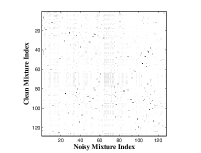
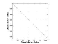
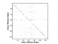
Figure 4.3.1a visualises such a matrix built using Aurora-2 stereo training data using $128$ mixture models. A dark spot in the plot represents a higher data count, and a bulk of stereo data points do belong to that mixture-pair.

In conventional SPLICE and M-SPLICE, only the noisy GMM $p(\mathbf{y})$ is built, and not $p(\mathbf{x})$. $p\left(m\,|\,\mathbf{y}_{n}\right)$ are computed for every noisy frame, and the same alignments are assumed for the clean frames $\{\mathbf{x}_{n}\}$ while computing $\boldsymbol{\mu}_{x,m}$ and $\boldsymbol{\Sigma}_{x,m}$. Hence $\boldsymbol{\mu}_{x,m}$, $\boldsymbol{\Sigma}_{x,m}$ and $p\left(m\,|\,\mathbf{y}\right)$ can be considered as the parameters of a clean hypothetical GMM $p(\mathbf{x})$. Now, given these GMMs $p(\mathbf{y})$ and $p(\mathbf{x})$, the matrix $\mathbf{V}$ can be constructed, which is visualised in Fig. (4.3.1b). Since the alignments are same, and $i^{th}$ clean mixture corresponds to the $i^{th}$ noisy mixture, a diagonal pattern can be seen.

Thus, under the assumption of Eq. (4.1.5), conventional SPLICE and M-SPLICE are able to estimate transforms from $i^{th}$ noisy mixture to exactly $i^{th}$ clean mixture by maintaining the mixture-correspondence.

When stereo not available, such exact mixture correspondence do not exist. Fig. 4.3.1a makes this fact evident, since stereo property was not used while building the two independent GMMs. However, a sparse structure can be seen, which suggests that for most noisy mixtures $j$, there exists a unique clean mixture $i^{*}$ having highest mixture-correspondence. This property can be exploited to estimate piecewise linear transformations from every mixture $j$ of $p(\mathbf{y})$ to a single mixture $i^{*}$ of $p(\mathbf{x})$, ignoring all other mixtures $i\neq i^{*}$. This is the basis for the proposed extension to non-stereo data.

4.3.2. Implementation

In the absence of stereo data, the approach is to build two separate GMMs viz., clean and noisy during training, such that there exists mixture-to-mixture correspondence between them, as close to Fig. 4.3.1b as possible. Then whitening based transforms can be estimated from each noisy mixture to its corresponding clean mixture. This sort of extension is not obvious in the conventional SPLICE framework, since it is not straight-forward to compute the cross-covariance terms $\boldsymbol{\Sigma}_{xy,m}$ without using stereo data. Also, M-SPLICE is expected to work better than SPLICE due to its advantages described earlier.

The training approach of two mixture-corresponded GMMs is as follows:

1. After building the noisy GMM $p(\mathbf{y})$, it is mean adapted by estimating a global MLLR transformation using clean training data. The transformed GMM has the same covariances and weights, and only means are altered to match the clean data. By this process, the mixture correspondences are not lost.

2. However, the transformed GMM need not model the clean data accurately. So a few (typically three) steps of expectation maximisation (EM) are performed using clean training data, initialising with the transformed GMM. This adjusts all the parameters and gives a more accurate representation of the clean GMM $p(\mathbf{x})$.

Now, the matrix obtained through this method using Aurora-2 training data is visualised in Figure 4.3.1c. It can be noted that no stereo information has been used while obtaining $p(\mathbf{x})$, following the above mentioned steps, from $p(\mathbf{y})$. It can be observed that a diagonal pattern is retained, as in the case of M-SPLICE, though there are some outliers. Since stereo information is not used, only comparable performances can be achieved. Figure 4.2.1b shows the block diagram of estimating transformations of non-stereo method. The steps are summarised as follows:

1. Build noisy GMM $p(\mathbf{y})$ using noisy features $\{\mathbf{y}\}$. This gives $\boldsymbol{\mu}_{y,m}$ and $\boldsymbol{\Sigma}_{y,m}$.

2. Adapt the means of noisy GMM $p(\mathbf{y})$ to clean data $\{\mathbf{x}\}$ using global MLLR transformation.

3. Perform at least three EM iterations to refine the adapted GMM using clean data. This gives $p(\mathbf{x})$, thus $\boldsymbol{\mu}_{x,m}$ and $\boldsymbol{\Sigma}_{x,m}$.

4. Compute $\mathbf{C}_{m}$ and $\mathbf{d}_{m}$ using Eq. (4.2.4) and (4.2.5).

The testing process is exactly same as that of M-SPLICE, as explained in Section 4.2.2.

4.4. Additional Run-time Adaptation

To improve the performance of the proposed methods during run-time, GMM adaptation to the test condition can be done in both conventional SPLICE and M-SPLICE frameworks in a simple manner. Conventional MLLR adaptation on HMMs involves two-pass recognition, where the transformation matrices are estimated using the alignments obtained through first pass Viterbi-decoded output, and a final recognition is performed using the transformed models.

MLLR adaptation can be used to adapt GMMs in the context of SPLICE and M-SPLICE as follows:

1. Adapt the noisy GMM through a global MLLR mean transformation

   $$\boldsymbol{\mu}_{y,m}^{(a)}\leftarrow\boldsymbol{\mu}_{y,m}$$

2. Now, adjust the bias term in conventional SPLICE or M-SPLICE as

   (4.4.1) $$\mathbf{d}_{m}^{(a)}=\boldsymbol{\mu}_{x,m}-\mathbf{C}_{m}\boldsymbol{\mu}_{y,m}^{(a)}$$

This method involves only simple calculation of alignments of the test data w.r.t. the noisy GMM, and doesn’t need Viterbi decoding. Clean mixture means $\mathbf{\mu}_{x,m}$ computed during training need to be stored. A separate global MLLR mean transform can be estimated using test utterances belonging to each noise condition. The steps for testing process for run-time compensation are summarised as follows:

1. For all test vectors $\{\mathbf{y}\}$ belonging to a particular environment, compute the alignments w.r.t. the noisy GMM, i.e., $p(m\,|\,\mathbf{y})$.

2. Estimate a global MLLR mean transformation using $\{\mathbf{y}\}$, maximising the likelihood w.r.t. $p(\mathbf{y})$.

3. Compute the adapted noisy GMM $p^{(a)}(\mathbf{y})$ using the estimated MLLR transform. Only the means $\boldsymbol{\mu}_{y,m}$ of the noisy GMM would have been adapted as $\boldsymbol{\mu}_{y,m}^{(a)}$.

4. Using Eq. (4.4.1), recompute the bias term of SPLICE or M-SPLICE.

5. Compute the cleaned test vectors as

   $$\widehat{\mathbf{x}}=\sum_{m=1}^{M}p\left(m\,|\,\mathbf{y}\right)\left(\mathbf{C}_{m}\mathbf{y}+\mathbf{d}_{m}^{(a)}\right)$$

4.5. Experiments and Results

4.5.1. Experimental Setup

All SPLICE based linear transformations have been applied on 13 dimensional MFCCs, including $C_{0}$. Aurora-2 setup is the same as described in 3.6.1. During HMM training, the features are appended with 13 delta and 13 acceleration coefficients to get a composite 39 dimensional vector per frame. Cepstral mean subtraction (CMS) has been performed in all the experiments. 128 mixture GMMs are built for all SPLICE based experiments. Run-time noise adaptation in SPLICE framework is performed on 13 dimensional MFCCs. Data belonging to each SNR level of a test noise condition has been separately used to compute the global transformations. In all SPLICE based experiments, pseudo-cleaning of clean features has been performed.

To test the efficacy of non-stereo method on a database which does not contain stereo data, Aurora-4 task of 8 kHz sampling frequency has been used. Aurora-4 is a continuous speech recognition task with clean and noisy training utterances (non-stereo) and test utterances of 14 environments. Aurora-4 acoustic models are built using crossword triphone HMMs of 3 states and 6 mixtures per state. Standard WSJ0 bigram language model has been used during decoding of Aurora-4. Noisy GMM of 512 mixtures is built for evaluating non-stereo method, using 7138 utterances taken from both clean and multi-training data. This GMM is adapted to standard clean training set to get the clean GMM.

4.5.2. Results

Table 4.1. SPLICE-based methods on Aurora-2 database

Noise Level	Baseline	SPLICE	M-SPLICE	M-SPLICE Diagonal	Non-Stereo Method	Non-Stereo Method Diagonal
Clean	99.25	98.97	99.01	98.98	99.08	99.03
SNR 20	97.35	97.84	97.92	97.85	97.68	97.67
SNR 15	93.43	95.81	96.10	95.78	95.15	95.01
SNR 10	80.62	89.48	91.03	90.19	87.37	86.74
SNR 5	51.87	72.71	77.59	75.46	68.49	67.35
SNR 0	24.30	42.85	50.72	46.60	39.00	37.76
SNR -5	12.03	18.52	22.27	19.39	16.73	16.31
Test A	67.45	81.39	83.47	81.72	77.44	76.64
Test B	72.26	83.24	84.18	82.43	79.63	79.06
Test C	68.14	69.42	78.06	77.57	73.54	73.13
Overall	69.51	79.74	82.67	81.17	77.54	76.91

(a) Individual Methods

Noise Level	MLLR (39)	SPLICE + RA	M-SPLICE + RA	M-SPLICE Diagonal + RA	Non-Stereo Method + RA	Non-Stereo Method Diagonal + RA
Clean	99.28	99.05	99.02	99.00	99.08	99.07
SNR 20	98.33	97.96	98.18	98.22	97.77	97.75
SNR 15	96.82	96.21	96.87	96.70	95.47	95.38
SNR 10	91.88	90.61	93.10	92.61	88.80	88.77
SNR 5	73.88	75.05	82.00	81.05	72.36	72.34
SNR 0	41.94	46.27	57.51	55.70	44.98	44.84
SNR -5	18.71	20.10	27.32	26.30	20.43	20.27
Test A	79.31	82.45	86.47	85.90	80.12	80.01
Test B	82.55	84.09	85.91	85.05	81.67	81.53
Test C	79.14	73.01	82.90	82.37	75.79	75.99
Overall	80.57	81.22	85.53	84.85	79.88	79.82

(b) Run-time adaptation

Table 4.2. Non-Stereo method on Aurora-4 database

		Clean	Car	Babble	Street	Restaurant	Airport	Station	Average
Baseline	Mic-1	87.63	75.58	52.77	52.83	46.53	56.38	45.30	54.73
	Mic-2	77.40	64.39	45.15	42.03	36.26	47.69	36.32
Non-Stereo Method	Mic-1	87.39	77.21	62.79	59.29	57.43	60.9	57.99	61.78
	Mic-2	78.95	67.18	55.41	50.72	46.31	54.55	48.76

(a) Clean-Training

		Clean	Car	Babble	Street	Restaurant	Airport	Station	Average
Baseline	Mic-1	86.89	82.83	70.52	68.52	65.37	72.73	64.28	70.16
	Mic-2	82.29	77.36	65.48	62.23	57.61	67.29	58.77
Non-Stereo Method	Mic-1	86.21	82.03	71.64	67.59	66.47	71.32	65.89	69.98
	Mic-2	80.59	75.68	66.41	62.11	58.68	65.31	59.85

(b) Multi-Training

Table 4.1a summarises the results of various algorithms discussed, on Aurora-2 dataset. All the results are shown in % accuracy. All SNRs levels mentioned are in decibels. The first seven rows report the overall results on all 10 test noise conditions. The rest of the rows report the average values in the SNR range $20-0$ dB. Table 4.2b shows the results of run-time adaptation (indicated as RA) using various methods. For reference, the result of standard MLLR adaptation on HMMs [Gales, 1998] has been shown in Table 4.2b, which computes a global 39 dimensional mean transformation, and uses two-pass Viterbi decoding. Table 4.2 shows the experimental results on Aurora-4 database. Table 4.2a shows the results of non-stereo method on Aurora-4 database using clean-trained HMMs. Table 4.2b shows the similar results for multi-trained HMMs, using the standard multi-training dataset.

It can be seen that M-SPLICE improves over SPLICE at all noise conditions and SNR levels and gives an absolute improvement of $8.6\%$ in test-set C and $2.93\%$ overall. Run-time compensation in SPLICE framework gives improvements over standard MLLR in test-sets A and B, whereas M-SPLICE gives improvements in all conditions. Here $9.89\%$ absolute improvement can be observed over SPLICE with run-time noise adaptation, and $4.96\%$ over standard MLLR. Finally, non-stereo method, though not using stereo data, shows $10.37\%$ and $7.05\%$ absolute improvements over Aurora-2 and Aurora-4 clean baseline models respectively, and a slight degradation w.r.t. SPLICE in all test cases. Run-time noise adaptation results of non-stereo method are comparable to that of standard MLLR, and are computationally less expensive. It can be observed that non-stereo method gives performance similar to that of multi-condition training.

4.6. Discussion

In terms of computational cost, the methods M-SPLICE and non-stereo methods are identical during testing as compared to conventional SPLICE. Also, there is almost negligible increase in cost during training. The MLLR mean adaptation in both non-stereo method and run-time adaptation are computationally very efficient, and do not need Viterbi decoding. The diagonal versions of the proposed methods give comparable performances.

In terms of performance, M-SPLICE is able to achieve good results in all cases without any use of adaptation data, especially in unseen cases. In non-stereo method, one-to-one mixture correspondence is assumed between noise and clean GMMs. The method gives slight degradation in performance. This could be attributed to neglecting the outlier data.

Comparing with other existing feature normalisation techniques, the techniques in SPLICE framework operate on individual feature vectors, and no estimation of parameters is required from test data. So these methods do not suffer from test data insufficiency problems, and are advantageous for shorter utterances. Also, the testing process is usually faster, and are easily implementable in real-time applications. So by extending the methods to non-stereo data, we believe that they become more useful in many applications.

Chapter 5 Conclusion and Future Work

In this thesis, feature normalisation methods suitable for noise robust real-time ASR have been studied. When there is no information about noise, it has been shown that an additional feature processing block in the MFCC extraction process can be included for noise-robustness. The additional block rebuilds all the speech frames from non-negative linear combinations of the speech subspace basis vectors in the LMFB domain. The new features are also shown to give improved performance when used with the existing techniques such as HEQ and HLDA.

In future, the methods may be improved by imposing sparseness constraints for learning better and more meaningful speech dictionaries. Also, the current methods involve iterative estimation of weights $\mathbf{H}$ during testing. Though the implementation is simple, owing to its slow convergence a large number of iterations is required. Addressing this issue could be another possible future work. The methods may be implemented in higher dimensional spaces for improvements, possibly involving DFT of larger number of samples during feature extraction.

In the presence of stereo training data, a modified version of the SPLICE algorithm has been proposed for noise robust ASR. It is better compliant with the assumptions of SPLICE, and improves the recognition in highly mismatched and unseen noise conditions. An extension of the methods to non-stereo data has been presented. Finally, a convenient run-time adaptation framework has been explained, which is computationally much cheaper than the standard MLLR adaptation of HMMs.

In future, the efficiency of the non-stereo extension of SPLICE can be improved. Better techniques could be proposed to achieve this, which either give fewer outliers in their mixture distribution plot, or do not neglect the outlier data. M-SPLICE could also be extended in uncertainty decoding framework, which has gained popularity [Droppo et al., 2002] over the conventional SPLICE.

Derivation of SPLICE Parameters

Let $\mathbf{W}_{m}=\begin{bmatrix}\mathbf{b}_{m}&\mathbf{A}_{m}\end{bmatrix}$ and $\mathbf{y}^{\prime}=\begin{bmatrix}1\\ \mathbf{y}\end{bmatrix}$. $\left(\mathbf{x}_{n},\mathbf{y}_{n}\right)$ can be substituted in

$$p(\mathbf{x}\,|\,\mathbf{y},m)\sim\mathcal{N}\left(\mathbf{x}\,;\,\mathbf{A}_{m}\mathbf{y}+\mathbf{b}_{m},\boldsymbol{\Sigma}_{x,m}\right)$$

to obtain

$$p\left(\mathbf{x}_{n}\,|\,\mathbf{y}_{n},m\right)=\frac{1}{\left(2\pi\right)^{\frac{D}{2}}\left|\boldsymbol{\Sigma}_{x,m}\right|^{\frac{1}{2}}}e^{-\frac{1}{2}\left(\mathbf{x}-\mathbf{W}_{m}\mathbf{y}_{n}^{\prime}\right)^{T}\boldsymbol{\Sigma}_{x,m}^{-1}\left(\mathbf{x}-\mathbf{W}_{m}\mathbf{y}_{n}^{\prime}\right)}$$

Now, the log-likelihood function can be expanded as

$$\mathcal{L}=\log\left[\prod_{n=1}^{N}p\left(\mathbf{x}_{n},\mathbf{y}_{n}\right)\right]=\sum_{n=1}^{N}\log\left[\sum_{m=1}^{M}p(\mathbf{x}_{n},\mathbf{y}_{n},m)\right]$$

$$\mathcal{L}=\sum_{n=1}^{N}\log\left[\sum_{m=1}^{M}p\left(\mathbf{x}_{n}\,|\,\mathbf{y}_{n},m\right)p\left(\mathbf{y}_{n}\,|\,m\right)P\left(m\right)\right]$$

Differentiating w.r.t $\mathbf{W}_{m}$ and equating to zero, and using the matrix identity

$$\frac{\partial}{\partial\mathbf{A}}\left(\mathbf{x}-\mathbf{A}\mathbf{s}\right)\mathbf{B}\left(\mathbf{x}-\mathbf{A}\mathbf{s}\right)=-2\mathbf{B}\left(\mathbf{x}-\mathbf{A}\mathbf{s}\right)\mathbf{s}^{T}$$

$$\implies\frac{\partial\mathcal{L}}{\partial\mathbf{W}_{m}}=\sum_{n=1}^{N}\frac{1}{p(\mathbf{x}_{n},\mathbf{y}_{n})}p\left(\mathbf{y}_{n}\,|\,m\right)P\left(m\right)p\left(\mathbf{x}_{n}\,|\,\mathbf{y}_{n},m\right)\boldsymbol{\Sigma}_{x,m}^{-1}\left(\mathbf{x}_{n}-\mathbf{W}_{m}\mathbf{y}_{n}^{\prime}\right)\mathbf{y}_{n}^{\prime T}=0$$

$$\implies\boldsymbol{\Sigma}_{x,m}^{-1}\left(\sum_{n=1}^{N}p\left(m\,|\,\mathbf{x}_{n},\mathbf{y}_{n}\right)\left(\mathbf{x}_{n}-\mathbf{W}_{m}\mathbf{y}_{n}^{\prime}\right)\mathbf{y}_{n}^{\prime T}\right)=0$$

SPLICE assumes a perfect correlation between $\mathbf{x}$ and $\mathbf{y}$, so

$$p\left(m\,|\,\mathbf{x}_{n},\mathbf{y}_{n}\right)\approx p\left(m\,|\,\mathbf{x}_{n}\right)\approx p\left(m\,|\,\mathbf{y}_{n}\right)$$

Since $\Gamma_{m}^{-1}$ is non-singular and the above matrix product is zero, it can be proved that

$$\sum_{n=1}^{N}p\left(m\,|\,\mathbf{y}_{n}\right)\left(\mathbf{x}_{n}-\mathbf{W}_{m}\mathbf{y}_{n}^{\prime}\right)\mathbf{y}_{n}^{\prime T}=0$$

Solving for $\mathbf{W}_{m}$ yields

$$\mathbf{W}_{m}=\left[\sum_{n=1}^{N}p\left(m\,|\,\mathbf{y}_{n}\right)\mathbf{x}_{n}\mathbf{y}_{n}^{\prime T}\right]\left[\sum_{n=1}^{N}p\left(m\,|\,\mathbf{y}_{n}\right)\mathbf{y}_{n}^{\prime}\mathbf{y}_{n}^{\prime T}\right]^{-1}$$

Publications Based on this Thesis

1. D. S. Pavan Kumar, N. Vishnu Prasad, Vikas Joshi, S. Umesh, “Modified SPLICE and its Extension to Non-Stereo Data for Noise Robust Speech Recognition,” accepted in IEEE Automatic Speech Recognition and Understanding Workshop, Olomouc, Dec. 2013. (View Online)

2. D. S. Pavan Kumar, Raghavendra Bilgi and S. Umesh, “Non-Negative Subspace Projection During Conventional MFCC Feature Extraction for Noise Robust Speech Recognition,” National Conference on Communications, New Delhi, Feb. 2013. (View Online)

References

- [Afify et al., 2009] Afify, M., Cui, X., and Gao, Y. (2009). Stereo-based stochastic mapping for robust speech recognition. IEEE Trans. on Audio, Speech and Lang. Proc., 17(7):1325–1334.
- [Chijiiwa et al., 2012] Chijiiwa, K., Suzuki, M., Minematsu, N., and Hirose, K. (2012). Unseen noise robust speech recognition using adaptive piecewise linear transformation. In Acoustics, Speech and Signal Processing (ICASSP), IEEE International Conference on, pages 4289–4292.
- [Deng et al., 2000] Deng, L., Acero, A., Plumpe, M., and Huang, X. (2000). Large-vocabulary speech recognition under adverse acoustic environments. In International Conference on Spoken Language Processing, pages 806–809.
- [Droppo and Acero, 2005] Droppo, J. and Acero, A. (2005). Maximum mutual information splice transform for seen and unseen conditions. In INTERSPEECH, pages 989–992.
- [Droppo et al., 2002] Droppo, J., Acero, A., and Deng, L. (2002). Uncertainty decoding with splice for noise robust speech recognition. In Acoustics, Speech, and Signal Processing (ICASSP), 2002 IEEE International Conference on, volume 1, pages I–57. IEEE.
- [Gales, 1998] Gales, M. J. (1998). Maximum likelihood linear transformations for hmm-based speech recognition. Computer speech & language, 12(2):75–98.
- [Gemmeke et al., 2011] Gemmeke, J. F., Virtanen, T., and Hurmalainen, A. (2011). Exemplar-based sparse representations for noise robust automatic speech recognition. IEEE Transactions on Audio, Speech & Language Processing, 19(7):2067–2080.
- [Gonzalez et al., 2011] Gonzalez, J., Peinado, A., Gomez, A., and Carmona, J. (2011). Efficient MMSE estimation and uncertainty processing for multienvironment robust speech recognition. Audio, Speech, and Language Processing, IEEE Transactions on, 19(5):1206–1220.
- [Hilger and Ney, 2006] Hilger, F. and Ney, H. (2006). Quantile based histogram equalization for noise robust large vocabulary speech recognition. IEEE Transactions on Audio, Speech and Language Processing, 14(3):845–854.
- [Hirsch and Pearce, 2000] Hirsch, H.-G. and Pearce, D. (2000). The aurora experimental framework for the performance evaluation of speech recognition systems under noisy conditions. In Automatic Speech Recognition: Challenges for the new Millenium ISCA Tutorial and Research Workshop (ITRW).
- [Kumar, 1997] Kumar, N. (1997). Investigation of Silicon Auditory Models and Generalization of Linear Discriminant Analysis for Improved Speech Recognition. PhD thesis, Johns Hopkins University.
- [Kumar and Andreou, 1998] Kumar, N. and Andreou, A. G. (1998). Heteroscedastic discriminant analysis and reduced rank hmms for improved speech recognition. Speech Communication, 26(4):283–297.
- [Lee and Seung, 1999] Lee, D. D. and Seung, H. S. (1999). Learning the parts of objects by non-negative matrix factorization. Nature, 401(6755):788–791.
- [Lee and Seung, 2000] Lee, D. D. and Seung, H. S. (2000). Algorithms for non-negative matrix factorization. In In NIPS, pages 556–562. MIT Press.
- [Legetter, 1995] Legetter, C. J. (1995). Improved acoustic modeling for HMMs using linear transformation. PhD thesis, University of Cambridge.
- [Rabiner and Schafer, 2010] Rabiner, L. and Schafer, R. (2010). Theory and Applications of Digital Speech Processing. Prentice Hall Press, Upper Saddle River, NJ, USA, 1st edition.
- [Sainath et al., 2012] Sainath, T., Ramabhadran, B., Nahamoo, D., Kanevsky, D., Van Compernolle, D., Demuynck, K., Gemmeke, J., Bellegarda, J., and Sundaram, S. (2012). Exemplar-based processing for speech recognition: An overview. IEEE Signal Processing Magazine, 29(6):98–113.
- [Schuller et al., 2010] Schuller, B., Weninger, F., Wollmer, M., Sun, Y., and Rigoll, G. (2010). Non-negative matrix factorization as noise-robust feature extractor for speech recognition. In Acoustics Speech and Signal Processing (ICASSP), IEEE International Conference on, pages 4562–4565.
- [Shinohara et al., 2008] Shinohara, Y., Masuko, T., and Akamine, M. (2008). Feature enhancement by speaker-normalized splice for robust speech recognition. In Acoustics, Speech and Signal Processing (ICASSP), IEEE International Conference on, pages 4881–4884. IEEE.
- [Smaragdis, 2007] Smaragdis, P. (2007). Convolutive speech bases and their application to supervised speech separation. Audio, Speech, and Language Processing, IEEE Transactions on, 15(1):1–12.
- [Wilson et al., 2008] Wilson, K., Raj, B., Smaragdis, P., and Divakaran, A. (2008). Speech denoising using nonnegative matrix factorization with priors. In Acoustics, Speech and Signal Processing (ICASSP), IEEE International Conference on, pages 4029–4032.
- [Young et al., 2009] Young, S. et al. (2009). The HTK book (revised for HTK version 3.4.1). Cambridge University.