Dirichlet-Neumann Waveform Relaxation Method for the 1D and 2D Heat and Wave Equations in Multiple subdomains

Abstract

We present a Waveform Relaxation (WR) version of the Dirichlet-Neumann algorithm, formulated specially for multiple subdomains splitting for general parabolic and hyperbolic problems. This method is based on a non-overlapping spatial domain decomposition, and the iteration involves subdomain solves in space-time with corresponding interface condition, and finally organize an exchange of information between neighboring subdomains. Using a Fourier-Laplace transform argument, for a particular relaxation parameter, we present convergence analysis of the algorithm for the heat and wave equations. We prove superlinear convergence for finite time window in case of the heat equation, and finite step convergence for the wave equation. The convergence behavior however depends on the size of the subdomains and the time window length on which the algorithm is employed. We illustrate the performance of the algorithm with numerical results, and show a comparison with classical and optimized Schwarz WR methods.

1 Introduction

A recent version of Waveform Relaxation (WR) methods, namely Dirichlet-Neumann Waveform Relaxation (DNWR) has been introduced in [16, 10, 9] to solve space-time problems in parallel computer. This iterative method is based on a non-overlapping domain decomoposition in space, and the iteration requires subdomain solves with Dirichlet boundary conditions followed by subdomain solves with Neumann boundary conditions. For a two-subdomain decomposition, we have proved superlinear convergence for 1D heat equation, and finite step convergence for 1D wave equation. In this paper, we extend the DNWR method to multiple subdomains, and present convergence analysis for one dimensional heat and wave equation. We also present convergence result for two dimensional wave equation.

In a different viewpoint, the WR-type methods can be seen as an extension of DD methods for elliptic PDEs. The systematic extension of the classical Schwarz method to time-dependent parabolic problems was started in [11, 12]; later optimized SWR methods have been introduced to achieve faster convergence or convergence with no overlap, see [6] for parabolic problems, and [7] for hyperbolic problems. Recently Neumann-Neumann Waveform Relaxation (NNWR) algorithm is formulated from substructuring-type Neumann-Neumann algorithm [2, 20, 22] to solve space-time problems; for more details see [13, 14, 15]. The DNWR method thus can be regarded as an extension of Dirichlet-Neumann (DN) method for solving elliptic problems. The DN algorithm was first considered by Bjørstad & Widlund [1] and further studied in [3], [17] and [18]. The performance of the algorithm is now well understood for elliptic problems, see for example the book [23] and the references therein.

We consider the following two PDEs on a bounded domain $\Omega\subset\mathbb{R}^{d},0<t<T$, $d=1,2,3$, with a smooth boundary as our guiding examples: the parabolic problem

$$\begin{array}[]{rcll}{\displaystyle\frac{\partial u}{\partial t}}&=&\nabla\cdot\left(\kappa(\boldsymbol{x},t)\nabla u\right)+f(\boldsymbol{x},t),&\boldsymbol{x}\in\Omega,\ 0<t<T,\\ u(\boldsymbol{x},0)&=&u_{0}(\boldsymbol{x}),&\boldsymbol{x}\in\Omega,\\ u(\boldsymbol{x},t)&=&g(\boldsymbol{x},t),&\boldsymbol{x}\in\partial\Omega,\ 0<t<T,\end{array}$$ (1)

where $\kappa(\boldsymbol{x},t)>0$, and the hyperbolic problem

$$\begin{array}[]{rcll}\frac{\partial^{2}u}{\partial t^{2}}-c^{2}(\boldsymbol{x})\Delta u&=&f(\boldsymbol{x},t),&\boldsymbol{x}\in\Omega,0<t<T,\\ u(\boldsymbol{x},0)&=&v_{0}(\boldsymbol{x}),&\boldsymbol{x}\in\Omega,\\ u_{t}(\boldsymbol{x},0)&=&w_{0}(\boldsymbol{x}),&\boldsymbol{x}\in\Omega,\\ u(\boldsymbol{x},t)&=&g(\boldsymbol{x},t),&\boldsymbol{x}\in\partial\Omega,0<t<T,\end{array}$$ (2)

with $c(\boldsymbol{x})$ being a positive function.

We introduce in Section 2 the non-overlapping DNWR algorithm with multiple subdomains for (1), and then analyze its convergence for the one dimensional heat equation. In Section 3 we define this method to hyperbolic problems, and analyze convergence behavior for one dimensional wave equation. We extend our result to two dimensional wave equation and prove similar convergence behavior as in 1D in Section 6. Finally we present numerical results in Section 7, which illustrate our analysis.

2 DNWR for parabolic problems

The Dirichlet-Neumann Waveform Relaxation (DNWR) method for parabolic problems with two subdomains is introduced in [10, 16]. In this section we generalize the algorithm to multiple subdomains in one spatial dimension. We present different possible arrangements (in terms of placing Dirichlet and Neumann boundary conditions) and with a numerical implementation of these arrangements for a model problem we determine the best possible one. We then formally define the DNWR method for (1), and analyze its convergence for the one dimensional heat equation.

2.1 Motivation

Suppose we want to solve the 1D heat equation

$$\begin{array}[]{rcll}{\displaystyle\frac{\partial u}{\partial t}}&=&\Delta u,&x\in\Omega,\ 0<t<T,\\ u(x,0)&=&u_{0}(x),&x\in\Omega,\\ u(x,t)&=&g(x,t),&x\in\partial\Omega,\ 0<t<T,\end{array}$$ (3)

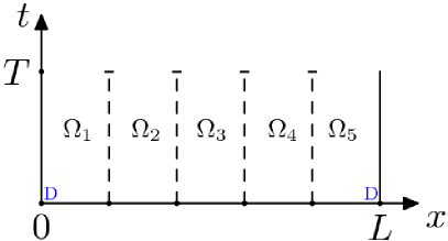
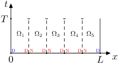
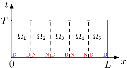
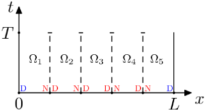
using the DNWR method. The spatial domain $\Omega=(0,5)$ is decomposed into five non-overlapping subdomains $\Omega_{i}=(x_{i-1},x_{i}),i=1,\ldots,5$, see the left panel of Figure 1, with three possible combinations of boundary conditions along the interfaces, right panel of Figure 1 and two arrangements in Figure 2. $D$ in blue denotes the Dirichlet condition along the two physical boundaries, whereas $D$ and $N$ in red denote the Dirichlet and Neumann boundary conditions along the interfaces. We are given Dirichlet traces $\left\{g_{i}^{0}(t)\right\}_{i=1}^{4}$ as initial guesses along the interfaces $\left\{x_{i}\right\}_{i=1}^{4}$.

First arrangement (A1):

Here we extend the two subdomain-formulation [10, 16] to many subdomains in a natural way, see the right panel of Figure 1. With the intial guesses, a Dirichlet subproblem is solved in the first subdomain $\Omega_{1}$, followed by a series of mixed Neumann-Dirichlet subproblem solves in the subsequent subdomains ($\Omega_{i},i=2,\ldots,5$), exactly like in the two-subdomain case. Thus the DNWR algorithm is given by: for $k=1,2\ldots$ and for $\theta\in(0,1]$ compute

$$\begin{array}[]{rcll}\partial_{t}u_{1}^{k}-\partial_{xx}u_{1}^{k}&=&0,&\textrm{in}\;\Omega_{1},t>0,\\ u_{1}^{k}(x,0)&=&u_{0}(x),&\textrm{in}\;\Omega_{1},\\ u_{1}^{k}(0,t)&=&g(0,t),&t>0,\\ u_{1}^{k}(x_{1},t)&=&g_{1}^{k-1}(t),&t>0,\end{array}$$

and for $i=2,\ldots,5$

$$\begin{array}[]{rcll}\partial_{t}u_{i}^{k}-\partial_{xx}u_{i}^{k}&=&0,&\textrm{in}\;\Omega_{i},t>0,\\ u_{i}^{k}(x,0)&=&u_{0}(x),&\textrm{in}\;\Omega_{i},\\ \partial_{x}u_{i}^{k}(x_{i-1},t)&=&\partial_{x}u_{i-1}^{k}(x_{i-1},t),&t>0,\\ u_{i}^{k}(x_{i},t)&=&g_{i}^{k-1}(t),&t>0,\end{array}$$

with $g_{5}^{k}(t)=g(5,t)$ for the last subdomain along the physical boundary. The updated interface values for the next step are then defined as

$$g_{i}^{k}(t)=\theta u_{i+1}^{k}(x_{i},t)+(1-\theta)g_{i}^{k-1}(t).$$

Fig. 1: Decomposition of the domain on the left, and arrangement of boundary conditions due to A1 on the right

Fig. 2: Two different arrangements of boundary conditions: A2 on the left, and A3 on the right

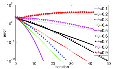
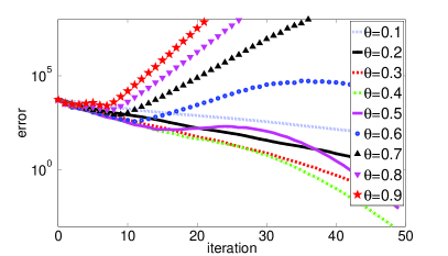
We now discretize (3) using standard centered finite differences in space and backward Euler in time, and solve the equation numerically using the above algorithm for different time windows. For the test we choose $u_{0}(x)=0,g(x,t)=(x+1)t,g_{i}^{0}(t)=t^{2},t\in[0,T]$. Figure 3 gives the convergence curves for different values of the parameter $\theta$ for $T=2$ on the left, and $T=20$ on the right.

Fig. 3: Arrangement A1: Convergence of multi-subdomain DNWR for various relaxation parameters $\theta$, on the left for $T=2$ and on the right for $T=20$

Second arrangement (A2):

This is the well-known red-black block formulation, described in the left panel of Figure 2. In this arrangement, we solve a Dirichlet subproblem and a Neumann subproblem in alternating fashion. Given initial Dirichlet traces along the interfaces, a series of Dirichlet subproblems is first solved in parallel in alternating subdomains ($\Omega_{1},\Omega_{3},\Omega_{5}$), and then a series of Neumann subproblems is solved in the remaining subdomains ($\Omega_{2},\Omega_{4}$). So this type of DNWR algorithm is given by: for $k=1,2\ldots$ compute for $i=1,3,5$

$$\begin{array}[]{rcll}\partial_{t}u_{i}^{k}-\partial_{xx}u_{i}^{k}&=&0,&\textrm{in}\;\Omega_{i},t>0,\\ u_{i}^{k}(x,0)&=&u_{0}(x),&\textrm{in}\;\Omega_{i},\\ u_{i}^{k}(x_{i-1},t)&=&g_{i-1}^{k-1}(t),&t>0,\\ u_{i}^{k}(x_{i},t)&=&g_{i}^{k-1}(t),&t>0,\end{array}$$

with $g_{0}^{k}(t)=g(0,t),g_{5}^{k}(t)=g(5,t)$, and for $i=2,4$

$$\begin{array}[]{rcll}\partial_{t}u_{i}^{k}-\partial_{xx}u_{i}^{k}&=&0,&\textrm{in}\;\Omega_{i},t>0,\\ u_{i}^{k}(x,0)&=&u_{0}(x),&\textrm{in}\;\Omega_{i},\\ \partial_{x}u_{i}^{k}(x_{i-1},t)&=&\partial_{x}u_{i-1}^{k}(x_{i-1},t),&t>0,\\ \partial_{x}u_{i}^{k}(x_{i},t)&=&\partial_{x}u_{i+1}^{k}(x_{i},t),&t>0,\end{array}$$

together with the updating conditions

$$g_{i}^{k}(t) = \theta u_{i+1}^{k}(x_{i},t)+(1-\theta)g_{i}^{k-1}(t),\;i=1,3,$$

$$g_{i}^{k}(t) = \theta u_{i}^{k}(x_{i},t)+(1-\theta)g_{i}^{k-1}(t),\;i=2,4,$$

where $\theta\in(0,1]$ is a relaxation parameter.

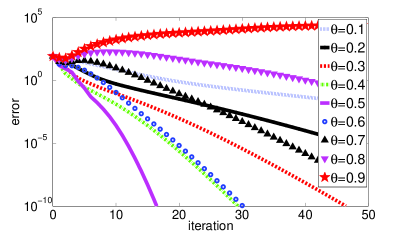
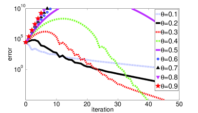
We now implement this version of DNWR algorithm for different time windows, picking the same problem and initial guesses as for A1. Figure 4 gives the convergence curves for different values of the parameter $\theta$ for $T=2$ on the left, and $T=20$ on the right.

Fig. 4: Arrangement A2: Convergence of multi-subdomain DNWR for various relaxation parameters $\theta$, on the left for $T=2$ and on the right for $T=20$

Third arrangement (A3):

We now consider a completely different type of arrangement, proposed in [4] and shown in the right panel of Figure 2. Given initial guesses along the interfaces, we begin with a Dirichlet solve in the middle subdomain $\Omega_{3}$, followed by mixed Neumann-Dirichlet subproblem solves in the adjacent subdomains, in an order $\Omega_{2},\Omega_{4}$ first and then in $\Omega_{1},\Omega_{5}$. This third version of the DNWR algorithms for multiple subdomains is given by: for $k=1,2\ldots$ and for $\theta\in(0,1]$ compute

$$\begin{array}[]{rcll}\partial_{t}u_{3}^{k}-\partial_{xx}u_{3}^{k}&=&0,&\textrm{in}\;\Omega_{3},t>0,\\ u_{3}^{k}(x,0)&=&u_{0}(x),&\textrm{in}\;\Omega_{3},\\ u_{3}^{k}(x_{2},t)&=&g_{2}^{k-1}(t),&t>0,\\ u_{3}^{k}(x_{3},t)&=&g_{3}^{k-1}(t),&t>0,\end{array}$$ (4)

and then for $i=2,1$

$$\begin{array}[]{rcll}\partial_{t}u_{i}^{k}-\partial_{xx}u_{i}^{k}&=&0,&\textrm{in}\;\Omega_{i},t>0,\\ u_{i}^{k}(x,0)&=&u_{0}(x),&\textrm{in}\;\Omega_{i},\\ u_{i}^{k}(x_{i-1},t)&=&g_{i-1}^{k-1}(t),&t>0,\\ \partial_{x}u_{i}^{k}(x_{i},t)&=&\partial_{x}u_{i+1}^{k}(x_{i},t),&t>0,\end{array}$$ (5)

and finally for $i=4,5$

$$\begin{array}[]{rcll}\partial_{t}u_{i}^{k}-\partial_{xx}u_{i}^{k}&=&0,&\textrm{in}\;\Omega_{i},t>0,\\ u_{i}^{k}(x,0)&=&u_{0}(x),&\textrm{in}\;\Omega_{i},\\ \partial_{x}u_{i}^{k}(x_{i-1},t)&=&\partial_{x}u_{i-1}^{k}(x_{i-1},t),&t>0,\\ u_{i}^{k}(x_{i},t)&=&g_{i}^{k-1}(t),&t>0,\end{array}$$ (6)

with $g_{0}^{k}(t)=g(0,t),g_{5}^{k}(t)=g(5,t)$ for the first and last subdomains at the physical boundaries. The updated interface values for the next step are defined as

$$g_{i}^{k}(t) = \theta u_{i}^{k}(x_{i},t)+(1-\theta)g_{i}^{k-1}(t),\;i=1,2,$$

$$g_{i}^{k}(t) = \theta u_{i+1}^{k}(x_{i},t)+(1-\theta)g_{i}^{k-1}(t),\;i=3,4.$$

We solve (3) using the above DNWR algorithm for different time windows for the same setting as in A1. Figure 5 gives the convergence curves for different values of the parameter $\theta$ for $T=2$ on the left, and $T=20$ on the right.

Fig. 5: Arrangement A3: Convergence of multi-subdomain DNWR for various relaxation parameters $\theta$, on the left for $T=2$ and on the right for $T=20$

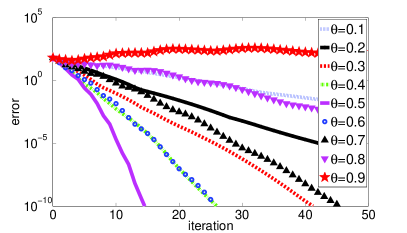
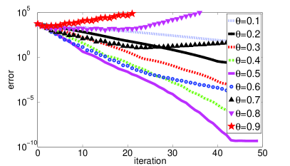
From the three numerical tests of the DNWR methods (A1, A2 and A3), it is evident that the behavior of these algorithms are similar for smaller time windows. But we notice clearly faster convergence for the arrangement A3 for large time windows. We therefore focus on the third version (A3) of the DNWR algorithms, and formally define the DNWR method for the general parabolic model problem (1) for multiple subdomains in the next subsection.

2.2 DNWR algorithm

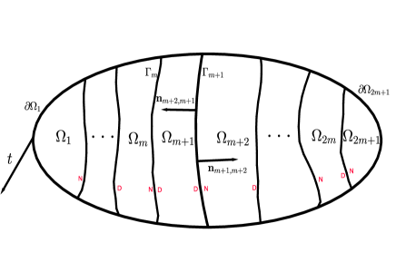
We now formally define the Dirichlet-Neumann Waveform Relaxation method for the model problem (1) on the space-time domain $\Omega\times(0,T)$ with Dirichlet data given on $\partial\Omega$. Suppose the spatial domain $\Omega$ is partitioned into $2m+1$ non-overlapping subdomains $\Omega_{i},i=1,\ldots,2m+1$ without any cross-points, as illustrated in Figure 6. We denote by $u_{i}$ the restriction of the solution $u$ of (1) to $\Omega_{i}$. For $i=1,\ldots,2m$, set $\Gamma_{i}:=\partial\Omega_{i}\cap\partial\Omega_{i+1}$. We further define $\Gamma_{0}=\Gamma_{2m+1}=\emptyset$. We denote by $\boldsymbol{n}_{i,j}$ the unit outward normal for $\Omega_{i}$ on the interface $\Gamma_{j},j=i-1,i$ (for $\Omega_{1},\Omega_{2m+1}$ we have only $\boldsymbol{n}_{1,2}$ and $\boldsymbol{n}_{2m+1,2m}$ respectively). In Figure 6, $D$ and $N$ in red denote the Dirichlet and Neumann boundary conditions respectively along the interfaces as in the arrangement A3.

The DNWR algorithm starts with initial Dirichlet traces $g_{i}^{0}(\boldsymbol{x},t)$ along the interfaces $\Gamma_{i}\times(0,T)$, $i=1,\ldots,2m$, and then performs the following computation for $k=1,2,\ldots$

$$\begin{array}[]{rcll}\partial_{t}u_{m+1}^{k}-\nabla\cdot\left(\kappa(\boldsymbol{x},t)\nabla u_{m+1}^{k}\right)&=&f,&\textrm{in}\;\Omega_{m+1},\\ u_{m+1}^{k}(\boldsymbol{x},0)&=&u_{0}(\boldsymbol{x}),&\textrm{in}\;\Omega_{m+1},\\ u_{m+1}^{k}&=&g,&\textrm{on}\;\partial\Omega\cap\partial\Omega_{m+1},\\ u_{m+1}^{k}&=&g_{i}^{k-1},&\textrm{on}\;\Gamma_{i},i=m,m+1,\end{array}$$ (7)

and then for $m\geq i\geq 1$ and $m+2\leq j\leq 2m+1$

$$\begin{array}[]{rcll}\partial_{t}u_{i}^{k}&=&\nabla\cdot\left(\kappa(\boldsymbol{x},t)\nabla u_{i}^{k}\right)+f,&\,\textrm{in}\;\Omega_{i},\\ u_{i}^{k}(\boldsymbol{x},0)&=&u_{0}(\boldsymbol{x}),&\textrm{in}\;\Omega_{i},\\ u_{i}^{k}&=&\widetilde{g}_{i}^{k-1},&\textrm{on}\;\partial\Omega_{i}\setminus\Gamma_{i},\\ \partial_{\boldsymbol{n}_{i,i+1}}u_{i}^{k}&=&-\partial_{\boldsymbol{n}_{i+1,i}}u_{i+1}^{k},&\textrm{on}\;\Gamma_{i},\end{array}\;\begin{array}[]{rcll}\partial_{t}u_{j}^{k}&=&\nabla\cdot\left(\kappa(\boldsymbol{x},t)\nabla u_{j}^{k}\right)+f,&\,\textrm{in}\;\Omega_{j},\\ u_{j}^{k}(\boldsymbol{x},0)&=&u_{0}(\boldsymbol{x}),&\textrm{in}\;\Omega_{j},\\ \partial_{\boldsymbol{n}_{j,j-1}}u_{j}^{k}&=&-\partial_{\boldsymbol{n}_{j-1,j}}u_{j-1}^{k},&\textrm{on}\;\Gamma_{j-1},\\ u_{j}^{k}&=&\check{g}_{j}^{k-1},&\textrm{on}\;\partial\Omega_{j}\setminus\Gamma_{j-1},\end{array}$$ (8)

with the update conditions along the interfaces

$$\begin{array}[]{rcl}g_{i}^{k}(\boldsymbol{x},t)&=&\theta u_{i}^{k}\left|{}_{\Gamma_{i}\times(0,T)}\right.+(1-\theta)g_{i}^{k-1}(\boldsymbol{x},t),\;1\leq i\leq m,\\ g_{j}^{k}(\boldsymbol{x},t)&=&\theta u_{j+1}^{k}\left|{}_{\Gamma_{j}\times(0,T)}\right.+(1-\theta)g_{j}^{k-1}(\boldsymbol{x},t),\;m+1\leq j\leq 2m,\end{array}$$ (9)

where $\theta\in(0,1]$, and for $i=1,\ldots,m$ and $j=m+2,\ldots,2m+1$

$$\widetilde{g}_{i}^{k-1}=\begin{cases}g,&\textrm{on}\;\partial\Omega\cap\partial\Omega_{i},\\ g_{i-1}^{k-1},&\textrm{on}\;\Gamma_{i-1},\end{cases},\quad\check{g}_{j}^{k-1}=\begin{cases}g,&\textrm{on}\;\partial\Omega\cap\partial\Omega_{j},\\ g_{j}^{k-1},&\textrm{on}\;\Gamma_{j},\end{cases}.$$

Fig. 6: Splitting into many non-overlapping strip-like subdomains

Remark 1.

The DNWR algorithm (7)-(8)-(9) is defined for an odd number of subdomains. In case of an even number of subdomains $2m+2$, we treat in a similar way as above the first $2m+1$ subdomains, keeping the last one aside. Then for the last subdomain, we apply a Neumann transmission condition along the interface $\Gamma_{2m+1}$ and a Dirichlet boundary condition along the physical boundary.

2.3 Convergence analysis

We present the convergence result of the DNWR algorithm (7)-(8)-(9) for the 1D heat equation with $\kappa(x,t)=\nu$. We split the domain $\Omega:=(0,L)$ into non-overlapping subdomains $\Omega_{i}:=(x_{i-1},x_{i})$, $i=1,\ldots,2m+1$, and define the subdomain length $h_{i}:=x_{i}-x_{i-1}$. Also, define the physical boundary conditions as $u(0,t)=g_{0}(t)$ and $u(L,t)=g_{L}(t)$, which in turn become zeros as we consider the error equations, $f(x,t)=0,g_{0}(t)=g_{L}(t)=0=u_{0}(x)$. We take $\left\{g_{i}^{0}(t)\right\}_{i=1}^{2m}$ as initial guesses along the interfaces $\left\{x=x_{i}\right\}\times(0,T)$, and for sake of consistency we denote $g_{0}^{k}(t)=g_{2m+1}^{k}=0$ for all $k$ corresponding to the physical boundaries. Denoting by $\left\{w_{i}^{k}(t)\right\}_{i=1}^{2m}$ for $k=1,2\ldots$ the Neumann traces along the interfaces, we compute

$$\begin{array}[]{rcll}\partial_{t}u_{m+1}^{k}-\nu\partial_{xx}u_{m+1}^{k}&=&0,&x\in\Omega_{m+1},\\ u_{m+1}^{k}(x,0)&=&0,&x\in\Omega_{m+1},\\ u_{m+1}^{k}(x_{m},t)&=&g_{m}^{k-1}(t),\\ u_{m+1}^{k}(x_{m+1},t)&=&g_{m+1}^{k-1}(t).\end{array}$$ (10)

and then for $m\geq i\geq 1$ and $m+2\leq j\leq 2m+1$

$$\begin{array}[]{rcll}\partial_{t}u_{i}^{k}-\nu\partial_{xx}u_{i}^{k}&=&0,&x\in\Omega_{i},\\ u_{i}^{k}(x,0)&=&0,&x\in\Omega_{i},\\ u_{i}^{k}(x_{i-1},t)&=&g_{i-1}^{k-1}(t),\\ \partial_{x}u_{i}^{k}(x_{i},t)&=&w_{i}^{k}(t),\end{array}\;\begin{array}[]{rcll}\partial_{t}u_{j}^{k}-\nu\partial_{xx}u_{j}^{k}&=&0,&x\in\Omega_{j},\\ u_{j}^{k}(x,0)&=&0,&x\in\Omega_{j},\\ -\partial_{x}u_{j}^{k}(x_{j-1},t)&=&w_{j-1}^{k}(t),\\ u_{j}^{k}(x_{j},t)&=&g_{j}^{k-1}(t),\end{array}$$ (11)

and finally the update conditions with the parameter $\theta\in(0,1]$

$$\begin{array}[]{rclrcl}g_{i}^{k}(t)&=&\theta u_{i}^{k}(x_{i},t)+(1-\theta)g_{i}^{k-1}(t),&w_{i}^{k}(t)&=&\partial_{x}u_{i+1}^{k}(x_{i},t),\;1\leq i\leq m,\\ g_{j}^{k}(t)&=&\theta u_{j+1}^{k}(x_{j},t)+(1-\theta)g_{j}^{k-1}(t),&w_{j}^{k}(t)&=&-\partial_{x}u_{j}^{k}(x_{j},t),\;m+1\leq j\leq 2m.\end{array}$$ (12)

We have the following main convergence result for DNWR for the heat equation and the proof will be given in Section 5.

Theorem 2 (Convergence of DNWR for multiple subdomains).

For $\theta=1/2$ and $T>0$ fixed, the DNWR algorithm (10)-(11)-(12) for multiple subdomains of unequal sizes $h_{i},1\leq i\leq 2m+1$ with $h_{\max}:=\max_{1\leq i\leq 2m+1}h_{i}$ and $h_{\min}:=\min_{1\leq i\leq 2m+1}h_{i}$ converges superlinearly with the estimate

$${\displaystyle\max_{1\leq i\leq 2m}}\parallel g_{i}^{k}\parallel_{L^{\infty}(0,T)}\leq\left(2m-3+\frac{2h_{\max}}{h_{m+1}}\right)^{k}{\rm erfc}\left(\frac{kh_{\min}}{2\sqrt{\nu T}}\right){\displaystyle\max_{1\leq i\leq 2m}}\parallel g_{i}^{0}\parallel_{L^{\infty}(0,T)}.$$

Remark 3.

The estimate in Theorem 2 holds for an odd number of subdomains. In case of an even number of subdomains $2m+2$, we define the algorithm as given in Remark 1, and the estimate will be of the form

$${\displaystyle\max_{1\leq i\leq 2m+1}}\parallel g_{i}^{k}\parallel_{L^{\infty}(0,T)}\leq\left(2m-1+\frac{2h_{\max}}{h_{m+1}}\right)^{k}{\rm erfc}\left(\frac{kh_{\min}}{2\sqrt{\nu T}}\right){\displaystyle\max_{1\leq i\leq 2m+1}}\parallel g_{i}^{0}\parallel_{L^{\infty}(0,T)}.$$ (13)

$2m-1$ appears in (13) as we calculate the estimate for $2m+3$ subdomains.

3 DNWR for hyperbolic problems

In this section we define the Dirichlet-Neumann Waveform Relaxation method with many subdomains for the model problem (2) on the space-time domain $\Omega\times(0,T)$. This can be treated as a generalization of the DNWR algorithm for two subdomains, for which see [9]. As before, there are three possible arrangements: A1, A2 and A3. However, for consistency we formally define below the DNWR algorithm for the arrangement A3.

3.1 DNWR algorithm

Suppose the spatial domain $\Omega$ is partitioned into $2m+1$ non-overlapping subdomains $\Omega_{i},i=1,\ldots,2m+1$, without any cross-points as illustrated in Figure 6. For $i=1,\ldots,2m$, set $\Gamma_{i}:=\partial\Omega_{i}\cap\partial\Omega_{i+1}$. For consistency, we set $\Gamma_{0}=\Gamma_{2m+1}=\emptyset$. We denote by $u_{i}$ the restriction of the solution $u$ of (2) to $\Omega_{i}$, and by $\boldsymbol{n}_{i,j}$ the unit outward normal for $\Omega_{i}$ on the interface $\Gamma_{j},j=i-1,i$ (for $\Omega_{1},\Omega_{2m+1}$ we have only $\boldsymbol{n}_{1,2}$ and $\boldsymbol{n}_{2m+1,2m}$ respectively). We define the DNWR method as in the arrangement A3, but one can also consider as in A1 and A2.

Given initial Dirichlet traces $g_{i}^{0}(\boldsymbol{x},t)$ along the interfaces $\Gamma_{i}\times(0,T)$, $i=1,\ldots,2m$, the DNWR algorithm consists of the following computation for $k=1,2,\ldots$

$$\begin{array}[]{rcll}\partial_{tt}u_{m+1}^{k}-c^{2}(\boldsymbol{x})\Delta u_{m+1}^{k}&=&f,&\textrm{in}\;\Omega_{m+1},\\ u_{m+1}^{k}(\boldsymbol{x},0)&=&v_{0}(\boldsymbol{x}),&\textrm{in}\;\Omega_{m+1},\\ \partial_{t}u_{m+1}^{k}(\boldsymbol{x},0)&=&w_{0}(\boldsymbol{x}),&\textrm{in}\;\Omega_{m+1},\\ u_{m+1}^{k}&=&g,&\textrm{on}\;\partial\Omega\cap\partial\Omega_{m+1},\\ u_{m+1}^{k}&=&g_{i}^{k-1},&\textrm{on}\;\Gamma_{i},i=m,m+1,\end{array}$$ (14)

and then for $m\geq i\geq 1$ and $m+2\leq j\leq 2m+1$

$$\begin{array}[]{rcll}\partial_{tt}u_{i}^{k}&=&c^{2}(\boldsymbol{x})\Delta u_{i}^{k}+f,&\,\textrm{in}\;\Omega_{i},\\ u_{i}^{k}(\boldsymbol{x},0)&=&v_{0}(\boldsymbol{x}),&\textrm{in}\;\Omega_{i},\\ \partial_{t}u_{i}^{k}(\boldsymbol{x},0)&=&w_{0}(\boldsymbol{x}),&\textrm{in}\;\Omega_{i},\\ u_{i}^{k}&=&\widetilde{g}_{i}^{k-1},&\textrm{on}\;\partial\Omega_{i}\setminus\Gamma_{i},\\ \partial_{\boldsymbol{n}_{i,i+1}}u_{i}^{k}&=&-\partial_{\boldsymbol{n}_{i+1,i}}u_{i+1}^{k},&\textrm{on}\;\Gamma_{i},\end{array}\;\begin{array}[]{rcll}\partial_{tt}u_{j}^{k}&=&c^{2}(\boldsymbol{x})\Delta u_{j}^{k}+f,&\,\textrm{in}\;\Omega_{j},\\ u_{j}^{k}(\boldsymbol{x},0)&=&v_{0}(\boldsymbol{x}),&\textrm{in}\;\Omega_{j},\\ \partial_{t}u_{j}^{k}(\boldsymbol{x},0)&=&w_{0}(\boldsymbol{x}),&\textrm{in}\;\Omega_{j},\\ \partial_{\boldsymbol{n}_{j,j-1}}u_{j}^{k}&=&-\partial_{\boldsymbol{n}_{j-1,j}}u_{j-1}^{k},&\textrm{on}\;\Gamma_{j-1},\\ u_{j}^{k}&=&\check{g}_{j}^{k-1},&\textrm{on}\;\partial\Omega_{j}\setminus\Gamma_{j-1},\end{array}$$ (15)

with the update conditions along the interfaces

$$\begin{array}[]{rcl}g_{i}^{k}(\boldsymbol{x},t)&=&\theta u_{i}^{k}\left|{}_{\Gamma_{i}\times(0,T)}\right.+(1-\theta)g_{i}^{k-1}(\boldsymbol{x},t),\;1\leq i\leq m,\\ g_{j}^{k}(\boldsymbol{x},t)&=&\theta u_{j+1}^{k}\left|{}_{\Gamma_{j}\times(0,T)}\right.+(1-\theta)g_{j}^{k-1}(\boldsymbol{x},t),\;m+1\leq j\leq 2m,\end{array}$$ (16)

where $\theta\in(0,1]$, and for $i=1,\ldots,m$ and $j=m+2,\ldots,2m+1$

$$\widetilde{g}_{i}^{k-1}=\begin{cases}g,&\textrm{on}\;\partial\Omega\cap\partial\Omega_{i},\\ g_{i-1}^{k-1},&\textrm{on}\;\Gamma_{i-1},\end{cases},\quad\check{g}_{j}^{k-1}=\begin{cases}g,&\textrm{on}\;\partial\Omega\cap\partial\Omega_{j},\\ g_{j}^{k-1},&\textrm{on}\;\Gamma_{j},\end{cases}.$$

3.2 Convergence analysis

We analyze the DNWR algorithm (14)-(15)-(16) for the 1D wave equation with a constant wave speed, $c(x)=c$. Consider a splitting of the domain $\Omega:=(0,L)$ into non-overlapping subdomains $\Omega_{i}:=(x_{i-1},x_{i})$, $i=1,\ldots,2m+1$, and define the subdomain length $g_{i}:=x_{i}-x_{i-1}$. As we consider the error equations, the physical boundary conditions $u(0,t)=g_{0}(t)$ and $u(L,t)=g_{L}(t)$ become zeros along with $f(x,t)=0,v_{0}(x)=0=w_{0}(x)$. We take $\left\{g_{i}^{0}(t)\right\}_{i=1}^{2m}$ as initial guesses along the interfaces $\left\{x=x_{i}\right\}\times(0,T)$, and for sake of consistency we denote $g_{0}^{k}(t)=g_{2m+1}^{k}=0$ for all $k$ corresponding to the physical boundaries. Denoting by $\left\{w_{i}^{k}(t)\right\}_{i=1}^{2m}$ for $k=1,2\ldots$ the Neumann traces along the interfaces, we compute

$$\begin{array}[]{rcll}\partial_{tt}u_{m+1}^{k}-c^{2}\partial_{xx}u_{m+1}^{k}&=&0,&x\in\Omega_{m+1},\\ u_{m+1}^{k}(x,0)&=&0,&x\in\Omega_{m+1},\\ \partial_{t}u_{m+1}^{k}(x,0)&=&0,&x\in\Omega_{m+1},\\ u_{m+1}^{k}(x_{m},t)&=&g_{m}^{k-1}(t),\\ u_{m+1}^{k}(x_{m+1},t)&=&g_{m+1}^{k-1}(t).\end{array}$$ (17)

and then for $m\geq i\geq 1$ and $m+2\leq j\leq 2m+1$

$$\begin{array}[]{rcll}\partial_{tt}u_{i}^{k}-c^{2}\partial_{xx}u_{i}^{k}&=&0,&x\in\Omega_{i},\\ u_{i}^{k}(x,0)&=&0,&x\in\Omega_{i},\\ \partial_{t}u_{i}^{k}(x,0)&=&0,&x\in\Omega_{i},\\ u_{i}^{k}(x_{i-1},t)&=&g_{i-1}^{k-1}(t),\\ \partial_{x}u_{i}^{k}(x_{i},t)&=&w_{i}^{k}(t),\end{array}\;\begin{array}[]{rcll}\partial_{tt}u_{j}^{k}-c^{2}\partial_{xx}u_{j}^{k}&=&0,&x\in\Omega_{j},\\ u_{j}^{k}(x,0)&=&0,&x\in\Omega_{j},\\ \partial_{t}u_{j}^{k}(x,0)&=&0,&x\in\Omega_{j},\\ -\partial_{x}u_{j}^{k}(x_{j-1},t)&=&w_{j-1}^{k}(t),\\ u_{j}^{k}(x_{j},t)&=&g_{j}^{k-1}(t),\end{array}$$ (18)

and finally the update conditions with the parameter $\theta\in(0,1]$

$$\begin{array}[]{rclrcl}g_{i}^{k}(t)&=&\theta u_{i}^{k}(x_{i},t)+(1-\theta)g_{i}^{k-1}(t),&w_{i}^{k}(t)&=&\partial_{x}u_{i+1}^{k}(x_{i},t),\;1\leq i\leq m,\\ g_{j}^{k}(t)&=&\theta u_{j+1}^{k}(x_{j},t)+(1-\theta)g_{j}^{k-1}(t),&w_{j}^{k}(t)&=&-\partial_{x}u_{j}^{k}(x_{j},t),\;m+1\leq j\leq 2m.\end{array}$$ (19)

We now state the main convergence result for DNWR for the wave equation. The proof of Theorem 4 will also be given in Section 5.

Theorem 4 (Convergence of DNWR for multiple subdomains).

Let $\theta=1/2$. Then the DNWR algorithm (17)-(18)-(19) converges in at most $k+1$ iterations for multiple subdomains, if the time window length $T$ satisfies $T/k\leq h_{\min}/c$, where $c$ is the wave speed.

4 Auxiliary results

We need a few auxiliary results related to Laplace transform to prove our main convergence results. We define the convolution of two functions $g,w:(0,\infty)\rightarrow\mathbb{R}$ by

$$(g*w)(t):=\int_{0}^{t}g(t-\tau)w(\tau)d\tau.$$

Lemma 5.

Let $g$ and $w$ be two real-valued functions in $(0,\infty)$ with $\hat{w}(s)=\mathcal{L}\left\{w(t)\right\}$ the Laplace transform of $w$. Then for $t\in(0,T)$, we have the following properties:

1. If $g(t)\geq 0$ and $w(t)\geq 0$, then $(g*w)(t)\geq 0$.

2. $\|g*w\|_{L^{1}(0,T)}\leq\|g\|_{L^{1}(0,T)}\|w\|_{L^{1}(0,T)}.$

3. $\bigl{|}(g*w)(t)\bigl{|}\leq\|g\|_{L^{\infty}(0,T)}\int_{0}^{T}\bigl{|}w(\tau)\bigl{|}d\tau.$

4. $\int_{0}^{t}w(\tau)d\tau=(H*w)(t)=\mathcal{L}^{-1}\left(\frac{\hat{w}(s)}{s}\right)$, $H(t)$ being the Heaviside step function.

Proof.

The proofs follow directly from the definitions. ∎

Lemma 6 (Limit).

Let, $w(t)$ be a continuous and $L^{1}$-integrable function on $(0,\infty)$ with $w(t)\geq 0$ for all $t\geq 0$, and $\hat{w}(s)=\mathcal{L}\left\{w(t)\right\}$ be its Laplace transform. Then, for $\tau>0$, we have the bound

$$\int_{0}^{\tau}|w(t)|dt\leq\lim_{s\rightarrow 0+}\hat{w}(s).$$

Proof.

For a proof of this lemma, see [10]. ∎

Lemma 7 (Positivity).

Let $\beta>\alpha\geq 0$ and $s$ be a complex variable. Then, for $t\in(0,\infty)$

$$\varphi(t):=\mathcal{L}^{-1}\left\{\frac{\sinh(\alpha\sqrt{s})}{\sinh(\beta\sqrt{s})}\right\}\geq 0\quad\mbox{and}\quad\psi(t):=\mathcal{L}^{-1}\left\{\frac{\cosh(\alpha\sqrt{s})}{\cosh(\beta\sqrt{s})}\right\}\geq 0.$$

Proof.

For a proof, we again cite [10]. ∎

Lemma 8.

Let $\alpha,\beta>0$ be two real numbers and $s$ be a complex variable. Set

$$\chi(s):=\frac{\sinh((\alpha-\beta)\sqrt{s})}{\cosh(\alpha\sqrt{s})\sinh(\beta\sqrt{s})}.$$ (20)

Then

$$\int_{0}^{T}\bigl{|}\mathcal{L}^{-1}\left\{\chi(\cdot)\right\}(\tau)\bigr{|}d\tau={\displaystyle\lim_{s\rightarrow 0+}}\chi(s)=\left|\frac{\alpha-\beta}{\beta}\right|.$$

Proof.

There are two possibilities: $\alpha>\beta$ or $\alpha<\beta$. In either case, we need Lemma 7 to prove positivity of the expression. For a detailed proof, see [10]. ∎

5 Proof of main results

We now prove the main convergence results for the DNWR algorithm applied to the heat and wave equations, stated in Section 2 and 3.

5.1 Proof of Theorem 2

We start by applying the Laplace transform to the homogeneous Dirichlet subproblem in (10), and obtain

$$s\hat{u}_{m+1}^{k}-\nu\hat{u}_{m+1,xx}^{k}=0,\quad\hat{u}_{m+1}^{k}(x_{m},s)=\hat{g}_{m}^{k-1}(s),\quad\hat{u}_{m+1}^{k}(x_{m+1},s)=\hat{g}_{m+1}^{k-1}(s),$$

Defining $\sigma_{i}:=\sinh\left(h_{i}\sqrt{s/\nu}\right)$ and $\gamma_{i}:=\cosh\left(h_{i}\sqrt{s/\nu}\right)$, the subproblem (10) solution becomes

$$\begin{array}[]{rcl}\hat{u}_{m+1}^{k}(x,s)&=&\frac{1}{\sigma_{m+1}}\left(\hat{g}_{m+1}^{k-1}(s)\sinh\left((x\!-\!x_{m})\sqrt{s/\nu}\right)\!+\!\hat{g}_{m}^{k-1}(s)\sinh\left((x_{m+1}\!-\!x)\sqrt{s/\nu}\right)\right).\end{array}$$

Similarly the solutions of the subproblems (11) in Laplace space are

$$\begin{array}[]{rcl}\hat{u}_{i}^{k}(x,s)&=&\frac{1}{\gamma_{i}}\frac{\hat{w}_{i}^{k}}{\sqrt{s/\nu}}\sinh((x-x_{i-1})\sqrt{s/\nu})+\frac{1}{\gamma_{i}}\hat{g}_{i-1}^{k-1}\cosh((x_{i}-x)\sqrt{s/\nu}),\\ \hat{u}_{j}^{k}(x,s)&=&\frac{1}{\gamma_{j}}\hat{g}_{j}^{k-1}\cosh((x-x_{j-1})\sqrt{s/\nu})+\frac{1}{\gamma_{j}}\frac{\hat{w}_{j-1}^{k}}{\sqrt{s/\nu}}\sinh((x_{j}-x)\sqrt{s/\nu}),\end{array}$$

for $1\leq i\leq m$ and $m+2\leq j\leq 2m+1$. Therefore for $\theta=1/2$ the update conditions (12) become

$$\begin{array}[]{rclrcl}\hat{g}_{i}^{k}&=&\frac{1}{2\gamma_{i}}\hat{g}_{i-1}^{k-1}+\frac{1}{2}\hat{g}_{i}^{k-1}+\frac{\sigma_{i}}{2\gamma_{i}}\frac{\hat{w}_{i}^{k}}{\sqrt{s/\nu}},&\hat{g}_{j}^{k}&=&\frac{\sigma_{j+1}}{2\gamma_{j+1}}\frac{\hat{w}_{j}^{k}}{\sqrt{s/\nu}}+\frac{1}{2}\hat{g}_{j}^{k-1}+\frac{1}{2\gamma_{j+1}}\hat{g}_{j+1}^{k-1},\end{array}$$ (21)

for $1\leq i\leq m$, $m+1\leq j\leq 2m$ and

$$\begin{array}[]{rcl}\hat{w}_{i}^{k}&=&-\sqrt{\frac{s}{\nu}}\frac{\sigma_{i+1}}{\gamma_{i+1}}\hat{g}_{i}^{k-1}+\frac{1}{\gamma_{i+1}}\hat{w}_{i+1}^{k},1\leq i\leq m-1;\;\hat{w}_{m}^{k}=-\sqrt{\frac{s}{\nu}}\frac{\gamma_{m+1}}{\sigma_{m+1}}\hat{g}_{m}^{k-1}+\frac{\sqrt{s/\nu}}{\sigma_{m+1}}\hat{g}_{m+1}^{k-1},\\ \hat{w}_{m+1}^{k}&=&\frac{\sqrt{s/\nu}}{\sigma_{m+1}}\hat{g}_{m}^{k-1}-\sqrt{\frac{s}{\nu}}\frac{\gamma_{m+1}}{\sigma_{m+1}}\hat{g}_{m+1}^{k-1};\quad\hat{w}_{j}^{k}=\frac{1}{\gamma_{j}}\hat{w}_{j-1}^{k}-\sqrt{\frac{s}{\nu}}\frac{\sigma_{j}}{\gamma_{j}}\hat{g}_{j}^{k-1},\;m+2\leq j\leq 2m.\end{array}$$ (22)

We choose $\bar{g}_{i}^{k}:=\gamma_{i}\hat{g}_{i}^{k}$, $\bar{w}_{i}^{k}:=\frac{\hat{w}_{i}^{k}}{\sqrt{s/\nu}}\sigma_{i},1\leq i\leq m$ and $\bar{g}_{j}^{k}:=\gamma_{j+1}\hat{g}_{j}^{k},\bar{w}_{j}^{k}:=\frac{\hat{w}_{j}^{k}}{\sqrt{s/\nu}}\sigma_{j+1},m+1\leq j\leq 2m$ with $\gamma_{0}=\gamma_{2m+2}=1$ in (21)-(22) to get

$$\begin{array}[]{rclrcl}\bar{g}_{i}^{k}&=&\frac{1}{2\gamma_{i-1}}\bar{g}_{i-1}^{k-1}\!+\!\frac{1}{2}\bar{g}_{i}^{k-1}\!+\!\frac{1}{2}\bar{w}_{i}^{k},\,1\leq i\leq m;&\bar{g}_{j}^{k}&=&\frac{1}{2}\bar{w}_{j}^{k}\!+\!\frac{1}{2}\bar{g}_{j}^{k-1}\!\!+\!\!\frac{1}{2\gamma_{j+2}}\bar{g}_{j+1}^{k-1},\,m+1\leq j\leq 2m,\end{array}$$

and for $1\leq i\leq m-1$ and $m+2\leq j\leq 2m$,

$$\begin{array}[]{rcl}\bar{w}_{i}^{k}&=&-\frac{\sigma_{i}\sigma_{i+1}}{\gamma_{i}\gamma_{i+1}}\bar{g}_{i}^{k-1}\!+\!\frac{\sigma_{i}}{\sigma_{i+1}\gamma_{i+1}}\bar{w}_{i+1}^{k};\;\bar{w}_{m}^{k}=-\frac{\sigma_{m}\gamma_{m+1}}{\gamma_{m}\sigma_{m+1}}\bar{g}_{m}^{k-1}\!+\!\frac{\sigma_{m}}{\sigma_{m+1}\gamma_{m+2}}\bar{g}_{m+1}^{k-1},\\ \bar{w}_{m+1}^{k}&=&\frac{\sigma_{m+2}}{\gamma_{m}\sigma_{m+1}}\bar{g}_{m}^{k-1}-\frac{\gamma_{m+1}\sigma_{m+2}}{\sigma_{m+1}\gamma_{m+2}}\bar{g}_{m+1}^{k-1};\quad\bar{w}_{j}^{k}=\frac{\sigma_{j+1}}{\gamma_{j}\sigma_{j}}\bar{w}_{j-1}^{k}-\frac{\sigma_{j}\sigma_{j+1}}{\gamma_{j}\gamma_{j+1}}\bar{g}_{j}^{k-1}.\end{array}$$

Therefore in matrix form, the system becomes

$$A\begin{pmatrix}\bar{g}_{1}^{k}\\ \bar{w}_{1}^{k}\\ \vdots\\ \vdots\\ \bar{g}_{m}^{k}\\ \bar{w}_{m}^{k}\\ \bar{w}_{m+1}^{k}\\ \bar{g}_{m+1}^{k}\\ \vdots\\ \vdots\\ \bar{w}_{2m}^{k}\\ \bar{g}_{2m}^{k}\end{pmatrix}=B\begin{pmatrix}\bar{g}_{1}^{k-1}\\ \vdots\\ \bar{g}_{m}^{k-1}\\ \bar{g}_{m+1}^{k-1}\\ \vdots\\ \bar{g}_{2m}^{k-1}\end{pmatrix},\>\textrm{where }A=\begin{pmatrix}L_{1}&\mathbf{0}\\ \mathbf{0}&L_{2}\end{pmatrix}_{4m\times 4m},$$

with

$$L_{1}=\begin{bmatrix}1&-\frac{1}{2}\\ &1&0&-\frac{\sigma_{1}}{\sigma_{2}\gamma_{2}}\\ &&1&-\frac{1}{2}\\ &&&1&0&-\frac{\sigma_{2}}{\sigma_{3}\gamma_{3}}\\ &&&&\ddots&\ddots\\ &&&&&1&0&-\frac{\sigma_{m-1}}{\sigma_{m}\gamma_{m}}\\ &&&&&&1&-\frac{1}{2}\\ &&&&&&&1\end{bmatrix},L_{2}=\begin{bmatrix}1\\ -\frac{1}{2}&1\\ -\frac{\sigma_{i+1}}{\sigma_{i}\gamma_{i}}&0&1\\ &&-\frac{1}{2}&1\\ &&\ddots&\ddots&\ddots\\ &&&&-\frac{1}{2}&1\\ &&&&-\frac{\sigma_{2m+1}}{\sigma_{2m}\gamma_{2m}}&0&1\\ &&&&&&-\frac{1}{2}&1\end{bmatrix},$$

and

$$B=\left[\begin{array}[]{cccc|cccc}\frac{1}{2}&&&\\ -\frac{\sigma_{1}\sigma_{2}}{\gamma_{1}\gamma_{2}}&&&\\ \frac{1}{2\gamma_{1}}&\frac{1}{2}&&\\ &-\frac{\sigma_{2}\sigma_{3}}{\gamma_{2}\gamma_{3}}&&\\ &\frac{1}{2\gamma_{2}}&\frac{1}{2}&\\ &&\ddots&\\ &&\frac{1}{2\gamma_{m-1}}&\frac{1}{2}\\ &&&-\frac{\sigma_{m}\gamma_{m+1}}{\gamma_{m}\sigma_{m+1}}&\frac{\sigma_{m}}{\sigma_{m+1}\gamma_{m+2}}\\ \hline\cr&&&\frac{\sigma_{m+2}}{\sigma_{m+1}\gamma_{m}}&-\frac{\sigma_{m+2}\gamma_{m+1}}{\gamma_{m+2}\sigma_{m+1}}\\ &&&&\frac{1}{2}&\frac{1}{2\gamma_{m+3}}\\ &&&&&-\frac{\sigma_{m+2}\sigma_{m+3}}{\gamma_{m+2}\gamma_{m+3}}\\ &&&&&\frac{1}{2}&\frac{1}{2\gamma_{m+4}}\\ &&&&&&\ddots\\ &&&&&&\frac{1}{2}&\frac{1}{2\gamma_{2m+1}}\\ &&&&&&&-\frac{\sigma_{2m}\sigma_{2m+1}}{\gamma_{2m}\gamma_{2m+1}}\\ &&&&&&&\frac{1}{2}\end{array}\right]_{4m\times 2m}.$$

Thus inverting $A$, we obtain

$$\begin{pmatrix}\bar{g}_{1}^{k}\\ \vdots\\ \bar{g}_{m}^{k}\\ \bar{g}_{m+1}^{k}\\ \vdots\\ \bar{g}_{2m}^{k}\end{pmatrix}=P\begin{pmatrix}\bar{g}_{1}^{k-1}\\ \vdots\\ \bar{g}_{m}^{k-1}\\ \bar{g}_{m+1}^{k-1}\\ \vdots\\ \bar{g}_{2m}^{k-1}\end{pmatrix},$$ (23)

where

$$P=\left(\begin{array}[]{c|c}K_{1}&K_{2}\\ \hline\cr K_{3}&K_{4}\end{array}\right)_{2m\times 2m},K_{1}=\begin{bmatrix}\frac{\gamma_{1,2}}{2\gamma_{1}\gamma_{2}}&-\frac{\sigma_{1}\sigma_{3}}{2\gamma_{2}^{2}\gamma_{3}}&\cdots&\frac{-\sigma_{1}\sigma_{m}}{2\gamma_{2}\ldots\gamma_{m-2}\gamma_{m-1}^{2}\gamma_{m}}&\frac{-\sigma_{1}\gamma_{m+1}}{2\gamma_{2}\ldots\gamma_{m-1}\gamma_{m}^{2}\sigma_{m+1}}\\ \frac{1}{2\gamma_{1}}&\frac{\gamma_{2,3}}{2\gamma_{2}\gamma_{3}}&\ddots&\frac{-\sigma_{2}\sigma_{m}}{2\gamma_{3}\ldots\gamma_{m-2}\gamma_{m-1}^{2}\gamma_{m}}&\frac{-\sigma_{2}\gamma_{m+1}}{2\gamma_{3}\ldots\gamma_{m-1}\gamma_{m}^{2}\sigma_{m+1}}\\ 0&\ddots&\ddots&\vdots&\vdots\\ \vdots&0&\frac{1}{2\gamma_{m-2}}&\frac{\gamma_{m-1,m}}{2\gamma_{m-1}\gamma_{m}}&-\frac{\sigma_{m-1}\gamma_{m+1}}{2\gamma_{m}^{2}\sigma_{m+1}}\\ 0&\cdots&0&\frac{1}{2\gamma_{m-1}}&\frac{\sigma_{m+1,m}}{2\sigma_{m+1}\gamma_{m}}\end{bmatrix},$$

$$K_{2}=\begin{bmatrix}\frac{\sigma_{1}}{2\gamma_{2}\ldots\gamma_{m}\sigma_{m+1}\gamma_{m+2}}&0&\cdots&\cdots&0\\ \frac{\sigma_{2}}{2\gamma_{3}\ldots\gamma_{m}\sigma_{m+1}\gamma_{m+2}}&\vdots&\vdots&\vdots&\vdots\\ \vdots&\vdots&\vdots&\vdots&\vdots\\ \frac{\sigma_{m-1}}{2\gamma_{m}\sigma_{m+1}\gamma_{m+2}}&\vdots&\vdots&\vdots&\vdots\\ \frac{\sigma_{m}}{2\sigma_{m+1}\gamma_{m+2}}&0&\cdots&\cdots&0\end{bmatrix},K_{3}=\begin{bmatrix}0&\cdots&\cdots&0&\frac{\sigma_{m+2}}{2\gamma_{m}\sigma_{m+1}}\\ \vdots&\vdots&\vdots&\vdots&\frac{\sigma_{m+3}}{2\gamma_{m}\sigma_{m+1}\gamma_{m+2}}\\ \vdots&\vdots&\vdots&\vdots&\vdots\\ \vdots&\vdots&\vdots&\vdots&\frac{\sigma_{2m}}{2\gamma_{m}\sigma_{m+1}\gamma_{m+2}\ldots\gamma_{2m-1}}\\ 0&\cdots&\cdots&0&\frac{\sigma_{2m+1}}{2\gamma_{m}\sigma_{m+1}\gamma_{m+2}\ldots\gamma_{2m}}\end{bmatrix},$$

$$K_{4}=\begin{bmatrix}\frac{\sigma_{m+1,m+2}}{2\sigma_{m+1}\gamma_{m+2}}&\frac{1}{2\gamma_{m+3}}&0&\cdots&0\\ -\frac{\sigma_{m+3}\gamma_{m+1}}{2\sigma_{m+1}\gamma_{m+2}^{2}}&\frac{\gamma_{m+2,m+3}}{2\gamma_{m+2}\gamma_{m+3}}&\frac{1}{2\gamma_{m+4}}&0&\vdots\\ \vdots&\vdots&\ddots&\ddots&0\\ \frac{-\sigma_{2m}\gamma_{m+1}}{2\sigma_{m+1}\gamma_{m+2}^{2}\gamma_{m+3}\ldots\gamma_{2m-1}}&\frac{-\sigma_{2m}\sigma_{m+2}}{2\gamma_{m+2}\gamma_{m+3}^{2}\gamma_{m+4}\ldots\gamma_{2m-1}}&\ddots&\frac{\gamma_{2m-1,2m}}{2\gamma_{2m-1}\gamma_{2m}}&\frac{1}{2\gamma_{2m+1}}\\ \frac{-\sigma_{2m+1}\gamma_{m+1}}{2\sigma_{m+1}\gamma_{m+2}^{2}\gamma_{m+3}\ldots\gamma_{2m}}&\frac{-\sigma_{2m+1}\sigma_{m+2}}{2\gamma_{m+2}\gamma_{m+3}^{2}\gamma_{m+4}\ldots\gamma_{2m}}&\cdots&-\frac{\sigma_{2m-1}\sigma_{2m+1}}{2\gamma_{2m-1}\gamma_{2m}^{2}}&\frac{\gamma_{2m,2m+1}}{2\gamma_{2m}\gamma_{2m+1}}\end{bmatrix},$$

with $\gamma_{i,j}=\cosh\left((h_{i}-h_{j})\sqrt{s/\nu}\right),\sigma_{i,j}=\sinh\left((h_{i}-h_{j})\sqrt{s/\nu}\right)$. Therefore we can write the first equation as:

$$\begin{array}[]{rcl}2\hat{g}_{1}^{k}&=&\frac{\gamma_{1,2}}{\gamma_{1}\gamma_{2}}\hat{g}_{1}^{k-1}\!-\!\frac{\sigma_{1}\sigma_{3}}{\gamma_{1}\gamma_{2}\gamma_{3}}\hat{g}_{2}^{k-1}\!-\!\cdots\!-\!\frac{\sigma_{1}\sigma_{m}}{\gamma_{1}\gamma_{2}\ldots\gamma_{m-1}\gamma_{m}}\hat{g}_{m-1}^{k-1}\!-\!\frac{\sigma_{1}\gamma_{m+1}}{\gamma_{1}\ldots\gamma_{m}\sigma_{m+1}}\hat{g}_{m}^{k-1}\!+\!\frac{\sigma_{1}}{\gamma_{1}\ldots\gamma_{m}\sigma_{m+1}}\hat{g}_{m+1}^{k-1}.\end{array}$$ (24)

So with the substitution $\hat{v}_{i}^{k}:=2^{k}\gamma^{k}\hat{g}_{i}^{k}$, $\gamma=\cosh\left(h_{\min}\sqrt{s/\nu}\right)$, we get

$$\begin{array}[]{rcl}\hat{v}_{1}^{k}&=&\frac{\gamma\gamma_{1,2}}{\gamma_{1}\gamma_{2}}\hat{v}_{1}^{k-1}\!-\!\frac{\gamma\sigma_{1}\sigma_{3}}{\gamma_{1}\gamma_{2}\gamma_{3}}\hat{v}_{2}^{k-1}\!-\!\cdots\!-\!\frac{\gamma\sigma_{1}\sigma_{m}}{\gamma_{1}\gamma_{2}\ldots\gamma_{m-1}\gamma_{m}}\hat{v}_{m-1}^{k-1}\!-\!\frac{\gamma\sigma_{1}\gamma_{m+1}}{\gamma_{1}\ldots\gamma_{m}\sigma_{m+1}}\hat{v}_{m}^{k-1}\!+\!\frac{\gamma\sigma_{1}}{\gamma_{1}\ldots\gamma_{m}\sigma_{m+1}}\hat{v}_{m+1}^{k-1}\\ &=:&\displaystyle{\sum_{i=1}^{m+1}}\hat{d}_{1,i}\hat{v}_{i}^{k-1}.\end{array}$$

Now using Lemma 7 and 6, we obtain

$$\int_{0}^{\infty}|d_{1,1}(t)|dt\leq\lim_{s\rightarrow 0+}\frac{\cosh(h_{\min}\sqrt{s/\nu})\cosh\left((h_{1}-h_{2})\sqrt{s/\nu}\right)}{\cosh(h_{2}\sqrt{s/\nu})\cosh(h_{1}\sqrt{s/\nu})}\leq 1,$$

so that using Lemma 5, part 3, we get

$$\left\|\mathcal{L}^{-1}\left(\hat{d}_{1,1}\,\hat{v}_{1}^{k-1}(s)\right)\right\|_{L^{\infty}(0,T)}\leq\|v_{1}^{k-1}\|_{L^{\infty}(0,T)}.$$

Moreover, we write for $j=2,\ldots,m-1$

$$\hat{d}_{1,j}\! = \!\frac{\gamma}{\gamma_{2}\ldots\gamma_{j}}\left(1-\frac{\sigma_{1}\sigma_{j+1}}{\gamma_{1}\gamma_{j+1}}-1\right)=\frac{\gamma\cosh\left((h_{1}-h_{j+1})\sqrt{s/\nu}\right)}{\gamma_{2}\ldots\gamma_{j}\gamma_{1}\gamma_{j+1}}-\frac{\gamma}{\gamma_{2}\ldots\gamma_{j}}$$

$$= \!\frac{\cosh\left((h_{\min}+h_{1}-h_{j+1})\sqrt{s/\nu}\right)+\cosh\left((h_{\min}-h_{1}+h_{j+1})\sqrt{s/\nu}\right)}{2\gamma_{2}\ldots\gamma_{j}\gamma_{1}\gamma_{j+1}}-\frac{\gamma}{\gamma_{2}\ldots\gamma_{j}}.$$

Now $-h_{j+1}\leq h_{\min}+h_{1}-h_{j+1}=h_{1}+h_{\min}-h_{j+1}\leq h_{1}$, so for the first term, we choose the pairing

$$\frac{1}{\gamma_{2}\ldots\gamma_{j}}\cdot\frac{1}{2\cosh(h_{j+1}\sqrt{s/\nu})}\cdot\frac{\cosh\left((h_{\min}+h_{1}-h_{j+1})\sqrt{s/\nu}\right)}{\cosh(h_{1}\sqrt{s/\nu})}$$

and

$$\frac{1}{\gamma_{2}\ldots\gamma_{j}}\cdot\frac{1}{2\cosh(h_{1}\sqrt{s/\nu})}\cdot\frac{\cosh\left((h_{\min}-h_{1}+h_{j+1})\sqrt{s/\nu}\right)}{\cosh(h_{j+1}\sqrt{s/\nu})}.$$

We therefore get by Lemma 7 and 6

$$\begin{array}[]{rcl}\int_{0}^{\infty}|d_{1,j}(t)|\,dt&\leq&{\displaystyle\lim_{s\rightarrow 0+}}\left(\frac{\cosh\left((h_{\min}+h_{1}-h_{j+1})\sqrt{s/\nu}\right)+\cosh\left((h_{\min}-h_{1}+h_{j+1})\sqrt{s/\nu}\right)}{2\gamma_{2}\ldots\gamma_{j}\gamma_{1}\gamma_{j+1}}+\frac{\gamma}{\gamma_{2}\ldots\gamma_{j}}\right)\\ &\leq&2,\end{array}$$

so that

$$\left\|\mathcal{L}^{-1}\left(\hat{d}_{1,j}\hat{v}_{j}^{k-1}(s)\right)\right\|_{L^{\infty}(0,T)}\leq 2\,\|v_{j}^{k-1}\|_{L^{\infty}(0,T)}.$$

Finally we write $\hat{d}_{1,m}=\frac{\gamma}{\gamma_{2}\ldots\gamma_{m}}\left(1-\frac{\sigma_{1}\gamma_{m+1}}{\gamma_{1}\sigma_{m+1}}-1\right)=-\frac{\gamma}{\gamma_{2}\ldots\gamma_{m}}\cdot K_{1}(s)-\frac{\gamma}{\gamma_{2}\ldots\gamma_{m}}$, where $K_{1}(s)=\frac{\sinh\left((h_{1}-h_{m+1})\sqrt{s/\nu}\right)}{\sinh(h_{m+1}\sqrt{s/\nu})\cosh(h_{1}\sqrt{s/\nu})}$, and write

$$\hat{d}_{1,m+1}=\frac{\sigma}{\sigma_{m+1}}\cdot\frac{1}{\gamma_{2}\ldots\gamma_{m}}\left(\frac{\sigma_{1}\gamma}{\gamma_{1}\sigma}-1+1\right)=\frac{\sigma}{\sigma_{m+1}}\cdot\frac{1}{\gamma_{2}\ldots\gamma_{m}}\cdot K_{2}(s)+\frac{\sigma}{\sigma_{m+1}}\cdot\frac{1}{\gamma_{2}\ldots\gamma_{m}},$$

where $\sigma=\sinh\left(h_{\min}\sqrt{s/\nu}\right)$, $K_{2}(s)=\frac{\sinh\left((h_{1}-h_{\min})\sqrt{s/\nu}\right)}{\sinh(h_{\min}\sqrt{s/\nu})\cosh(h_{1}\sqrt{s/\nu})}$. Note that both $K_{1}(s)$ and $K_{2}(s)$ are of the form (20). So by Lemma 8, we obtain the bounds

$$\int_{0}^{\infty}|d_{1,m}(t)|\,dt\leq\lim_{s\rightarrow 0+}\frac{\gamma}{\gamma_{2}\ldots\gamma_{m}}\left(K_{1}(s)+1\right)\leq\bigl{|}\frac{h_{1}-h_{m+1}}{h_{m+1}}\bigr{|}+1,$$

and

$$\int_{0}^{\infty}|d_{1,m+1}(t)|dt\leq\lim_{s\rightarrow 0+}\frac{\sigma}{\sigma_{m+1}}\cdot\frac{1}{\gamma_{2}\ldots\gamma_{m}}\left(K_{2}(s)\!+\!1\right)\leq\frac{h_{\min}}{h_{m+1}}\left(\!\frac{h_{1}\!-\!h_{\min}}{h_{\min}}+1\!\right)\!=\!\frac{h_{1}}{h_{m+1}}.$$

We therefore get

$$\left\|v_{1}^{k}(\cdot)\right\|_{L^{\infty}(0,T)} \leq \left(1+2(m-2)+\frac{2h_{\max}}{h_{m+1}}\right){\displaystyle\max_{1\leq j\leq m+1}}\parallel v_{j}^{k-1}(\cdot)\parallel_{L^{\infty}(0,T)}$$

$$\leq \left(2m-3+\frac{2h_{\max}}{h_{m+1}}\right){\displaystyle\max_{1\leq j\leq 2m}}\parallel v_{j}^{k-1}(\cdot)\parallel_{L^{\infty}(0,T)}.$$

We also get similar relations for other equations. By induction, we therefore get for all $i$

$$\left\|v_{i}^{k}(\cdot)\right\|_{L^{\infty}(0,T)} \leq \left(2m-3+\frac{2h_{\max}}{h_{m+1}}\right){\displaystyle\max_{1\leq j\leq 2m}}\parallel v_{j}^{k-1}(\cdot)\parallel_{L^{\infty}(0,T)}$$ (25)

$$\leq \cdots\leq\left(2m-3+\frac{2h_{\max}}{h_{m+1}}\right)^{k}{\displaystyle\max_{1\leq j\leq 2m}}\parallel g_{j}^{0}(\cdot)\parallel_{L^{\infty}(0,T)}.$$

Setting $f_{k}(t):=\mathcal{L}^{-1}\left\{\frac{1}{\gamma^{k}}\right\}$ we have

$$g_{i}^{k}(t)=\frac{1}{2^{k}}\left(f_{k}*v_{i}^{k}\right)(t)=\frac{1}{2^{k}}\int_{0}^{t}f_{k}(t-\tau)v_{i}^{k}(\tau)d\tau,$$

from which it follows, using part 3 of Lemma 5 that

$$\|g_{i}^{k}(\cdot)\|_{L^{\infty}(0,T)}\leq\frac{1}{2^{k}}\|v_{i}^{k}(\cdot)\|_{L^{\infty}(0,T)}\int_{0}^{T}|f_{k}(\tau)|d\tau.$$ (26)

By Lemma 7, $f_{k}(t)\geq 0$ for all $t$. To obtain a bound for $\int_{0}^{T}f_{k}(\tau)\,d\tau$, we first show that the function $r_{k}(t)=\mathcal{L}^{-1}(2^{k}e^{-kh_{\min}\sqrt{s/\nu}})$ is greater than or equal to $f_{k}(t)$ for all $t>0$, and then bound $\int_{0}^{T}r_{k}(\tau)\,d\tau$ instead. Indeed, we have

$$\mathcal{L}\left\{r_{k}(t)-f_{k}(t)\right\} =2^{k}e^{-kh_{\min}\sqrt{s/\nu}}-\frac{2^{k}}{(e^{h_{\min}\sqrt{s/\nu}}+e^{-h_{\min}\sqrt{s/\nu}})^{k}}$$

$$=\frac{2^{k}((1+e^{-2h_{\min}\sqrt{s/\nu}})^{k}-1)}{(e^{h_{\min}\sqrt{s/\nu}}+e^{-h_{\min}\sqrt{s/\nu}})^{k}}$$

$$=\sum_{j=1}^{k}{k\choose j}e^{-2jh_{\min}\sqrt{s/\nu}}\operatorname{sech}^{k}(h_{\min}\sqrt{s/\nu}).$$

Also, by [19]

$$\mathcal{L}^{-1}\left(e^{-2jh_{\min}\sqrt{s/\nu}}\right)=\frac{jh_{\min}}{\sqrt{\pi\nu t^{3}}}e^{-j^{2}h_{\min}^{2}/\nu t},$$ (27)

is a positive function for $j=1,\ldots,k$. Thus, $\mathcal{L}^{-1}\left(e^{-2jh_{\min}\sqrt{s/\nu}}\operatorname{sech}^{k}(h_{\min}\sqrt{s/\nu})\right)$ is a convolution of positive functions, and hence positive by part 1 of Lemma 5. This implies $r_{k}(t)-f_{k}(t)\geq 0$, so we deduce that

$$\int_{0}^{T}f_{k}(\tau)\,d\tau\leq\int_{0}^{T}r_{k}(\tau)\,d\tau=\mathcal{L}^{-1}\left(\frac{2^{k}e^{-kh_{\min}\sqrt{s/\nu}}}{s}\right)=2^{k}\,\textrm{erfc}\left(\frac{kh_{\min}}{2\sqrt{\nu T}}\right),$$ (28)

where we expressed the second integral as an inverse Laplace transform using Lemma 5, part 4, which we then evaluated using the following identity from [19]:

$$\mathcal{L}^{-1}\left(\frac{1}{s}e^{-\lambda\sqrt{s}}\right)=\textrm{erfc}\left(\frac{\lambda}{2\sqrt{t}}\right),\quad\lambda>0.$$ (29)

Finally, we combine the above bound (28) with (25) and (26) to conclude the proof of the theorem.

Remark 9.

For equal subdomains, with subdomain size $h$, we can deduce a better estimate:

$${\displaystyle\max_{1\leq i\leq 2m}}\parallel g_{i}^{k}\parallel_{L^{\infty}(0,T)}\leq\left(\min\left\{2m-1,Q(h,\nu,T)\right\}\right)^{k}{\rm erfc}\left(\frac{kh}{2\sqrt{\nu T}}\right){\displaystyle\max_{1\leq i\leq 2m}}\parallel g_{i}^{0}\parallel_{L^{\infty}(0,T)},$$

where $Q(h,\nu,T):=2\,{\rm erfc}\left(\frac{h}{2\sqrt{\nu T}}\right)+\sum_{i=0}^{\infty}2^{i+1}{\rm erfc}\left(\frac{ih}{2\sqrt{\nu T}}\right)$.

Here is the outline of the proof: For equal-length subdomains we have $h_{i}=h$ for $i=1,\ldots,2m+1$, so that $\gamma_{i}=\gamma,\sigma_{i}=\sigma$ and $\gamma_{i,j}=1,\sigma_{i,j}=0$ for all $i,j$ in the matrix $P$ in (23). Therefore, the first update equation (24) becomes

$$\hat{g}_{1}^{k}=\frac{1}{2\gamma^{2}}\hat{g}_{1}^{k-1}-\frac{\sigma^{2}}{2\gamma^{3}}\hat{g}_{2}^{k-1}-\cdots-\frac{\sigma^{2}}{2\gamma^{m}}\hat{g}_{m-1}^{k-1}-\frac{1}{2\gamma^{m-1}}\hat{g}_{m}^{k-1}+\frac{1}{2\gamma^{m}}\hat{g}_{m+1}^{k-1},\;m\geq 2,$$ (30)

which in turn becomes after setting $\hat{v}_{i}^{k}(s)=2^{k}\gamma^{k}\hat{g}_{i}^{k}(s)$,

$$\hat{v}_{1}^{k}\!\! = \!\!\frac{1}{\gamma}\hat{v}_{1}^{k-1}-\left(1-\frac{1}{\gamma^{2}}\right)\hat{v}_{2}^{k-1}-\cdots-\frac{1}{\gamma^{m-3}}\left(1-\frac{1}{\gamma^{2}}\right)\hat{v}_{m-1}^{k-1}-\frac{1}{\gamma^{m-2}}\hat{v}_{m}^{k-1}+\frac{1}{\gamma^{m-1}}\hat{v}_{m+1}^{k-1}$$ (31)

$$=: \!\!\sum_{i=1}^{m+1}\hat{r}_{i}\hat{v}_{i}^{k-1}.$$

Note that the estimate from Theorem 2 also holds in this case with $h_{\max}=h_{m+1}$:

$${\displaystyle\max_{1\leq i\leq 2m}}\parallel g_{i}^{k}\parallel_{L^{\infty}(0,T)}\leq\left(2m-1\right)^{k}{\rm erfc}\left(\frac{kh}{2\sqrt{\nu T}}\right){\displaystyle\max_{1\leq i\leq 2m}}\parallel g_{i}^{0}\parallel_{L^{\infty}(0,T)}.$$ (32)

We now present a different estimate starting from (31). By back transforming into the time domain we obtain $v_{1}^{k}(t)=\sum_{i=1}^{m+1}\left(r_{i}*v_{i}^{k-1}\right)(t).$ Now part 3 of Lemma 5 yields

$$\|v_{1}^{k}\|_{L^{\infty}(0,T)} \leq \sum_{i=1}^{m+1}\|v_{i}^{k-1}\|_{L^{\infty}(0,T)}\int_{0}^{T}\!|r_{i}(\tau)|d\tau$$ (33)

$$\leq {\displaystyle\max_{1\leq i\leq m+1}}\parallel v_{i}^{k-1}\parallel_{L^{\infty}(0,T)}\sum_{i=1}^{m+1}\int_{0}^{T}\!|r_{i}(\tau)|d\tau.$$

Set $f_{k}(t):=\mathcal{L}^{-1}\left(\frac{1}{\gamma^{k}}\right)$. Since $\lim_{s\rightarrow 0+}\left|1-\frac{1}{\gamma^{2}}\right|\leq 2$, we have from (33)

$$\sum_{i=1}^{m+1}\int_{0}^{T}|r_{i}(\tau)|d\tau\leq\int_{0}^{T}\left(f_{1}(t)+2+2f_{1}(t)+\cdots+2f_{m-3}(t)+f_{m-2}(t)+f_{m-1}(t)\right)dt.$$

Therefore using the inequality (28), $\int_{0}^{T}f_{k}(t)dt\leq 2^{k}{\rm erfc}\left(\frac{kh}{2\sqrt{\nu T}}\right)$, the above expression is bounded by

$$\sum_{i=1}^{m+1}\int_{0}^{T}|r_{i}(\tau)|d\tau\leq 2\,{\rm erfc}\left(\frac{h}{2\sqrt{\nu T}}\right)+\sum_{i=0}^{m-1}2^{i+1}{\rm erfc}\left(\frac{ih}{2\sqrt{\nu T}}\right)\leq Q(h,\nu,T),$$

where $Q(h,\nu,T):=2\,{\rm erfc}\left(\frac{h}{2\sqrt{\nu T}}\right)+\sum_{i=0}^{\infty}2^{i+1}{\rm erfc}\left(\frac{ih}{2\sqrt{\nu T}}\right)$. So we get the second estimate as

$${\displaystyle\max_{1\leq i\leq 2m}}\parallel g_{i}^{k}\parallel_{L^{\infty}(0,T)}\leq Q^{k}\,{\rm erfc}\left(\frac{kh}{2\sqrt{\nu T}}\right){\displaystyle\max_{1\leq i\leq 2m}}\parallel g_{i}^{0}\parallel_{L^{\infty}(0,T)}.$$ (34)

The result follows combining the two estimates (32) and (34).

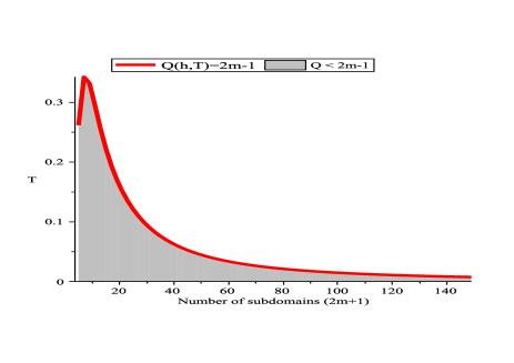
We compare the two estimates (32) and (34) in Figure 7 for $\nu=1$. The region below the red curve is where the estimate (32) is more accurate than (34).

Fig. 7: Comparison of the two estimates (32) and (34) for $\nu=1$

5.2 Proof of Theorem 4

We start by applying the Laplace transform to the homogeneous Dirichlet subproblem in (17) to get

$$s^{2}\hat{u}_{m+1}^{k}-c^{2}\hat{u}_{m+1,xx}^{k}=0,\quad\hat{u}_{m+1}^{k}(x_{m},s)=\hat{g}_{m}^{k-1}(s),\quad\hat{u}_{m+1}^{k}(x_{m+1},s)=\hat{g}_{m+1}^{k-1}(s),$$

Define $\rho_{i}:=\sinh\left(h_{i}s/c\right)$ and $\lambda_{i}:=\cosh\left(h_{i}s/c\right)$. Then the subproblem (17) solution becomes

$$\hat{u}_{m+1}^{k}(x,s)=\frac{1}{\rho_{m+1}}\left(\hat{g}_{m+1}^{k-1}(s)\sinh\left((x-x_{m})s/c\right)+\hat{g}_{m}^{k-1}(s)\sinh\left((x_{m+1}-x)s/c\right)\right).$$

The solutions of the subproblems (18) in Laplace space are

$$\begin{array}[]{rcl}\hat{u}_{i}^{k}(x,s)&=&\frac{1}{\lambda_{i}}\frac{\hat{w}_{i}^{k}}{s/c}\sinh((x-x_{i-1})s/c)+\frac{1}{\lambda_{i}}\hat{g}_{i-1}^{k-1}\cosh((x_{i}-x)s/c),\;1\leq i\leq m,\\ \hat{u}_{j}^{k}(x,s)&=&\frac{1}{\lambda_{j}}\hat{g}_{j}^{k-1}\cosh((x-x_{j-1})s/c)+\frac{1}{\lambda_{j}}\frac{\hat{w}_{j-1}^{k}}{s/c}\sinh((x_{j}-x)s/c),\;m+2\leq j\leq 2m+1.\end{array}$$

Therefore for $\theta=1/2$ the update conditions (19) become

$$\begin{array}[]{rcl}\hat{g}_{i}^{k}&=&\frac{1}{2\lambda_{i}}\hat{g}_{i-1}^{k-1}+\frac{1}{2}\hat{g}_{i}^{k-1}+\frac{\rho_{i}}{2\lambda_{i}}\frac{\hat{w}_{i}^{k}}{s/c},\;1\leq i\leq m,\\ \hat{g}_{j}^{k}&=&\frac{\rho_{j+1}}{2\lambda_{j+1}}\frac{\hat{w}_{j}^{k}}{s/c}+\frac{1}{2}\hat{g}_{j}^{k-1}+\frac{1}{2\lambda_{j+1}}\hat{g}_{j+1}^{k-1},\;m+1\leq j\leq 2m.\end{array}$$ (35)

and

$$\begin{array}[]{rcl}\hat{w}_{i}^{k}&=&-\frac{s}{c}\frac{\rho_{i+1}}{\lambda_{i+1}}\hat{g}_{i}^{k-1}+\frac{1}{\lambda_{i+1}}\hat{w}_{i+1}^{k},1\leq i\leq m-1;\;\hat{w}_{m}^{k}=-\frac{s}{c}\frac{\lambda_{m+1}}{\rho_{m+1}}\hat{g}_{m}^{k-1}+\frac{s/c}{\rho_{m+1}}\hat{g}_{m+1}^{k-1},\\ \hat{w}_{m+1}^{k}&=&\frac{s/c}{\rho_{m+1}}\hat{g}_{m}^{k-1}-\frac{s}{c}\frac{\lambda_{m+1}}{\rho_{m+1}}\hat{g}_{m+1}^{k-1};\quad\hat{w}_{j}^{k}=\frac{1}{\lambda_{j}}\hat{w}_{j-1}^{k}-\frac{s}{c}\frac{\rho_{j}}{\lambda_{j}}\hat{g}_{j}^{k-1},\;m+2\leq j\leq 2m,\end{array}$$ (36)

We choose $\bar{g}_{i}^{k}:=\lambda_{i}\hat{g}_{i}^{k},\bar{w}_{i}^{k}:=\frac{\hat{w}_{i}^{k}}{s/c}\rho_{i},1\leq i\leq m$ and $\bar{g}_{j}^{k}:=\lambda_{j+1}\hat{g}_{j}^{k},\bar{w}_{j}^{k}:=\frac{\hat{w}_{j}^{k}}{s/c}\rho_{j+1},m+1\leq j\leq 2m$ with $\lambda_{0}=\lambda_{2m+2}=1$ in the corresponding equations of (35)-(36) to get

$$\begin{array}[]{rcl}{g}_{i}^{k}&=&\frac{1}{2\lambda_{i-1}}\bar{g}_{i-1}^{k-1}+\frac{1}{2}\bar{g}_{i}^{k-1}+\frac{1}{2}\bar{w}_{i}^{k},\;1\leq i\leq m;\\ \bar{g}_{j}^{k}&=&\frac{1}{2}\bar{w}_{j}^{k}+\frac{1}{2}\bar{g}_{j}^{k-1}+\frac{1}{2\lambda_{j+2}}\bar{g}_{j+1}^{k-1},\;m+1\leq j\leq 2m,\end{array}$$

and for $1\leq i\leq m-1$ and $m+2\leq j\leq 2m$,

$$\begin{array}[]{rcl}\bar{w}_{i}^{k}&=&-\frac{\rho_{i}\rho_{i+1}}{\lambda_{i}\lambda_{i+1}}\bar{g}_{i}^{k-1}+\frac{\rho_{i}}{\rho_{i+1}\lambda_{i+1}}\bar{w}_{i+1}^{k};\;\bar{w}_{m}^{k}=-\frac{\rho_{m}\lambda_{m+1}}{\lambda_{m}\rho_{m+1}}\bar{g}_{m}^{k-1}+\frac{\rho_{m}}{\rho_{m+1}\lambda_{m+2}}\bar{g}_{m+1}^{k-1},\\ \bar{w}_{m+1}^{k}&=&\frac{\rho_{m+2}}{\lambda_{m}\rho_{m+1}}\bar{g}_{m}^{k-1}-\frac{\lambda_{m+1}\rho_{m+2}}{\rho_{m+1}\lambda_{m+2}}\bar{g}_{m+1}^{k-1};\quad\bar{w}_{j}^{k}=\frac{\rho_{j+1}}{\lambda_{j}\rho_{j}}\bar{w}_{j-1}^{k}-\frac{\rho_{j}\rho_{j+1}}{\lambda_{j}\lambda_{j+1}}\bar{g}_{j}^{k-1}.\end{array}$$

Therefore we can write the system in matrix form as in the Heat equation case

$$\begin{pmatrix}\bar{g}_{1}^{k}\\ \vdots\\ \bar{g}_{m}^{k}\\ \bar{g}_{m+1}^{k}\\ \vdots\\ \bar{g}_{2m}^{k}\end{pmatrix}=P\begin{pmatrix}\bar{g}_{1}^{k-1}\\ \vdots\\ \bar{g}_{m}^{k-1}\\ \bar{g}_{m+1}^{k-1}\\ \vdots\\ \bar{g}_{2m}^{k-1}\end{pmatrix},$$

where $P$ is in the same form as in (23) with $\gamma_{i,j}$ and $\sigma_{i,j}$ replaced by $\lambda_{i,j}:=\cosh\left((h_{i}-h_{j})s/c\right),\rho_{i,j}:=\sinh\left((h_{i}-h_{j})s/c\right)$ respectively. Therefore the updating conditions become

$$\hat{g}_{i}^{k}(s)={\displaystyle\sum_{l=i-1}^{m+1}}\hat{k}_{i,l}\hat{g}_{l}^{k-1}(s),\>1\leq i\leq m;\quad\hat{g}_{j}^{k}(s)={\displaystyle\sum_{l=m}^{j+1}}\hat{k}_{j,l}\hat{g}_{l}^{k-1}(s),\>m+1\leq j\leq 2m,$$ (37)

where $\hat{k}_{1,0}=\hat{k}_{2m,2m+1}=0$, and for $i+1\leq l<m$ $\hat{k}_{i,i-1}=\frac{1}{2\lambda_{i}},\hat{k}_{i,i}=\frac{\lambda_{i,i+1}}{2\lambda_{i}\lambda_{i+1}},\hat{k}_{i,l}=-\frac{\rho_{i}\rho_{l+1}}{2\lambda_{i}\lambda_{i+1}\ldots\lambda_{l+1}},$ $\hat{k}_{i,m}=-\frac{\rho_{i}\lambda_{m+1}}{2\lambda_{i}\ldots\lambda_{m}\rho_{m+1}},\hat{k}_{i,m+1}=\frac{\rho_{i}}{2\lambda_{i}\ldots\lambda_{m}\rho_{m+1}}$ for $1\leq i<m,$ and for $m+1<l\leq j-1$ $\hat{k}_{j,j}=\frac{\lambda_{j,j+1}}{2\lambda_{j}\lambda_{j+1}},\hat{k}_{j,l}=-\frac{\rho_{j+1}\rho_{l}}{2\lambda_{l}\lambda_{l+1}\ldots\lambda_{j+1}},\hat{k}_{j,j+1}=\frac{1}{2\lambda_{j+1}},$ $\hat{k}_{j,m+1}=-\frac{\rho_{j+1}\lambda_{m+1}}{2\rho_{m+1}\lambda_{m+2}\ldots\lambda_{j+1}},\hat{k}_{j,m}=\frac{\rho_{j+1}}{2\rho_{m+1}\lambda_{m+2}\ldots\lambda_{j+1}}$ for $m+1<j\leq 2m.$ Also, $\hat{k}_{m,m-1}=\frac{1}{2\lambda_{m}},\hat{k}_{m,m}=\frac{\rho_{m+1,m}}{2\rho_{m+1}\lambda_{m}},\hat{k}_{m,m+1}=\frac{\rho_{m}}{2\rho_{m+1}\lambda_{m}}$ and $\hat{k}_{m+1,m}=\frac{\rho_{m+2}}{2\rho_{m+1}\lambda_{m+2}},\hat{k}_{m+1,m+1}=\frac{\rho_{m+1,m+2}}{2\rho_{m+1}\lambda_{m+2}},\hat{k}_{m+1,m+2}=\frac{1}{2\lambda_{m+2}}.$ So by induction on (37) we can write for $1\leq i\leq 2m$

$$\hat{g}_{i}^{k}(s)=\sum_{j=1}^{2m}p_{i,j}^{n}\left(\hat{k}_{1,1},\hat{k}_{1,2},\ldots,\hat{k}_{2m,2m-1},\hat{k}_{2m,2m}\right)\,\hat{g}_{j}^{k-n}(s),$$ (38)

where the coefficients $p_{i,j}^{n}$ are either zero or homogeneous polynomials of degree $n$. Now expanding hyperbolic functions into infinite binomial series, we obtain for $i+1\leq l<m$ and $1\leq i<m$

$$\hat{k}_{i,i}=\frac{\cosh\left((h_{i}-h_{i+1})s/c\right)}{2\cosh(h_{i}s/c)\cosh(h_{i+1}s/c)}=\left(e^{-2h_{i}s/c}+e^{-2h_{i+1}s/c}\right)\left[1+{\displaystyle\sum_{l=1}^{\infty}}(-1)^{l}e^{-2h_{i}ls/c}\right.\\ \left.+{\displaystyle\sum_{n=1}^{\infty}}(-1)^{n}e^{-2h_{i+1}ns/c}+{\displaystyle\sum_{l=1}^{\infty}}{\displaystyle\sum_{n=1}^{\infty}}(-1)^{l+n}e^{-2(lh_{i}+nh_{i+1})s/c}\right],$$

$$\hat{k}_{i,l}=-\frac{\sinh\left(h_{i}s/c\right)\sinh\left(h_{l+1}s/c\right)}{2\cosh(h_{i}s/c)\cosh(h_{i+1}s/c)\ldots\cosh(h_{l+1}s/c)}=-2^{l-i-1}e^{-\left(h_{i+1}+\cdots+h_{l}\right)s/c}\left(1-\right.\\ \left.e^{-2h_{i}s/c}-e^{-2h_{l+1}s/c}+e^{-2(h_{i}+h_{l+1})s/c}\right){\displaystyle\prod_{n=i}^{l+1}}\left(1+e^{-2h_{n}s/c}\right)^{-1},$$

$$\hat{k}_{i,i-1}=\frac{1}{2\cosh(h_{i}s/c)}=e^{-h_{i}s/c}\left[1+{\displaystyle\sum_{l=1}^{\infty}}(-1)^{l}e^{-2h_{i}ls/c}\right],$$

$$\hat{k}_{i,m}=-\frac{\sinh\left(h_{i}s/c\right)\cosh\left(h_{m+1}s/c\right)}{2\cosh(h_{i}s/c)\ldots\cosh(h_{m}s/c)\sinh(h_{m+1}s/c)}\\ =-2^{m-i-1}e^{-\left(h_{i+1}+\cdots+h_{m}\right)s/c}\left(1-e^{-2h_{i}s/c}+e^{-2h_{m+1}s/c}\right.\\ \left.-e^{-2(h_{i}+h_{m+1})s/c}\right)\left(1-e^{-2h_{m+1}s/c}\right)^{-1}{\displaystyle\prod_{l=i}^{m}}\left(1+e^{-2h_{l}s/c}\right)^{-1},$$

$$\hat{k}_{i,m+1}=\frac{\sinh\left(h_{i}s/c\right)}{2\cosh(h_{i}s/c)\ldots\cosh(h_{m}s/c)\sinh(h_{m+1}s/c)}\\ =2^{m-i}e^{-\left(h_{i+1}+\cdots+h_{m+1}\right)s/c}\left(1-e^{-2h_{i}s/c}\right)\left(1-e^{-2h_{m+1}s/c}\right)^{-1}{\displaystyle\prod_{l=i}^{m}}\left(1+e^{-2h_{l}s/c}\right)^{-1},$$

$$\hat{k}_{m,m}=\frac{\sinh\left((h_{m+1}-h_{m})s/c\right)}{2\cosh(h_{m}s/c)\sinh(h_{m+1}s/c)}=\left(e^{-2h_{m}s/c}-e^{-2h_{m+1}s/c}\right)\left[1\right.\\ \left.+{\displaystyle\sum_{l=1}^{\infty}}(-1)^{l}e^{-2h_{m}ls/c}+{\displaystyle\sum_{n=1}^{\infty}}e^{-2h_{m+1}ns/c}+{\displaystyle\sum_{l=1}^{\infty}}{\displaystyle\sum_{n=1}^{\infty}}(-1)^{l}e^{-2(lh_{m}+nh_{m+1})s/c}\right],$$

$$\hat{k}_{m,m+1}=\frac{\sinh\left(h_{m}s/c\right)}{2\cosh(h_{m}s/c)\sinh(h_{m+1}s/c)}=\left(e^{-h_{m+1}s/c}-e^{-(2h_{m}+h_{m+1})s/c}\right)\left[1\right.\\ \left.+{\displaystyle\sum_{l=1}^{\infty}}(-1)^{l}e^{-2h_{m}ls/c}+{\displaystyle\sum_{n=1}^{\infty}}e^{-2h_{m+1}ns/c}+{\displaystyle\sum_{l=1}^{\infty}}{\displaystyle\sum_{n=1}^{\infty}}(-1)^{l}e^{-2(lh_{m}+nh_{m+1})s/c}\right].$$

The argument also holds similarly for other terms. Now using these expressions we can write (38) as

$$\hat{g}_{i}^{k}(s)=\sum_{j=1}^{2m}\hat{r}_{i,j}^{k}(s)\,\hat{g}_{j}^{0}(s),$$ (39)

where $\hat{r}_{i,j}^{k}(s)$ are linear combinations of terms of the form $e^{-sz}$ with $z\geq kh_{l}/c$ for some $l\in\left\{1,2,\ldots 2m+1\right\}$. We now recall the shifting property of Laplace transform:

$$\mathcal{L}^{-1}\left\{e^{-\alpha s}\hat{f}(s)\right\}=H(t-\alpha)f(t-\alpha),$$ (40)

where $H(t):=\begin{cases}1,&t>0,\\ 0,&t\leq 0.\end{cases}$ is the Heaviside step function. We use (40) to back transform (39) and obtain

$$g_{i}^{k}(t)=g_{j}^{0}\left(t-\frac{kh_{l}}{c}\right)H\left(t-\frac{kh_{l}}{c}\right)+\>\textrm{other terms},$$

for some $j\in\left\{1,2,\ldots 2m\right\}$ and $l\in\left\{1,2,\ldots 2m+1\right\}$. Thus for $T\leq kh_{\min}/c$, we get $g_{i}^{k}(t)=0$ for all $i$, and the conclusion follows.

Remark 10.

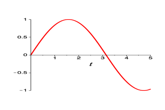
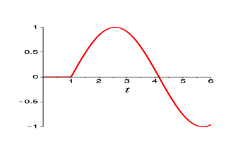
The shifting property of Laplace transform (40) is the reason behind the finite step convergence of the DNWR for $\theta=1/2$. The right hand side of (40) becomes identically zero for $t\leq\alpha$, so that for sufficiently small time window length $T$ (e.g., $T\leq\alpha$) the error becomes zero and leads to convergence in the next iteration. In Figure 8 we plot $\mathcal{L}^{-1}\left\{\hat{f}(s)\right\}$ with $f(t)=\sin(t)$ on the left, and show the effect of time-shifting on the right.

Fig. 8: Example of time-shifting for the function $f(t)=\sin(t)$: $\mathcal{L}^{-1}\left\{\hat{f}(s)\right\}$ on the left, and $\mathcal{L}^{-1}\left\{e^{-s}\hat{f}(s)\right\}$ on the right

6 Analysis of DNWR algorithm for Wave equation in 2D

We now formulate and analyze the DNWR algorithm for the two-dimensional wave equation

$$\partial_{tt}u-c^{2}\Delta u=f(x,y,t),\quad(x,y)\in\Omega=(l,L)\times(0,\pi),\>t\in(0,T]$$

with initial condition $u(x,y,0)=v_{0}(x,y),\partial_{t}u(x,y,0)=w_{0}(x,y)$ and Dirichlet boundary conditions $u(x,y,t)=g(x,y,t),(x,y)\in\partial\Omega$. To define the DNWR algorithm, we decompose $\Omega$ into strips of the form $\Omega_{i}=(x_{i-1},x_{i})\times(0,\pi)$, $l=x_{0}<x_{1}<\cdots<x_{2m+1}=L$. We define the subdomain width $h_{i}:=x_{i}-x_{i-1}$, and $h_{\min}:=\min_{1\leq i\leq 2m+1}h_{i}$. Also we directly consider the error equations with $f(x,y,t)=0,v_{0}(x,y)=0=w_{0}(x,y)$ and homogeneous Dirichlet boundary conditions. Given initial guesses $\left\{g_{i}^{0}(y,t)\right\}_{i=1}^{2m}$ along the interface $\left\{x=x_{i}\right\}$, the DNWR algorithm, as a particular case of (14)-(15)-(16), is given by performing iteratively for $k=1,2,\ldots$

$$\begin{array}[]{rcll}\partial_{tt}u_{m+1}^{k}-c^{2}\Delta u_{m+1}^{k}&=&0,&\textrm{in}\;\Omega_{m+1},\\ u_{m+1}^{k}(x,y,0)&=&0,&\textrm{in}\;\Omega_{m+1},\\ \partial_{t}u_{m+1}^{k}(x,y,0)&=&0,&\textrm{in}\;\Omega_{m+1},\\ u_{m+1}^{k}(x_{m},y,t)&=&g_{m}^{k-1}(y,t),&\\ u_{m+1}^{k}(x_{m+1},y,t)&=&g_{m+1}^{k-1}(y,t),&\\ u_{m+1}^{k}(x,0,t)&=&u_{m+1}^{k}(x,\pi,t)=0,&\end{array}$$ (41)

and then denoting by $\left\{w_{i}^{k}(y,t)\right\}_{i=1}^{2m}$ the Neumann traces along the interfaces, calculate for $m\geq i\geq 1$ and $m+2\leq j\leq 2m+1$

$$\begin{array}[]{rcll}\partial_{tt}u_{i}^{k}-c^{2}\Delta u_{i}^{k}&=&0,&\textrm{in}\;\Omega_{i},\\ u_{i}^{k}(x,y,0)&=&0,&\textrm{in}\;\Omega_{i},\\ \partial_{t}u_{i}^{k}(x,y,0)&=&0,&\textrm{in}\;\Omega_{i},\\ u_{i}^{k}(x_{i-1},y,t)&=&g_{i-1}^{k-1}(y,t),&\\ \partial_{x}u_{i}^{k}(x_{i},y,t)&=&w_{i}^{k}(y,t),&\\ u_{i}^{k}(x,0,t)&=&u_{i}^{k}(x,\pi,t)=0,&\end{array}\;\begin{array}[]{rcll}\partial_{tt}u_{j}^{k}-c^{2}\Delta u_{j}^{k}&=&0,&\textrm{in}\;\Omega_{j},\\ u_{j}^{k}(x,y,0)&=&0,&\textrm{in}\;\Omega_{j},\\ \partial_{t}u_{j}^{k}(x,y,0)&=&0,&\textrm{in}\;\Omega_{j},\\ -\partial_{x}u_{j}^{k}(x_{j-1},y,t)&=&w_{j-1}^{k}(y,t),&\\ u_{j}^{k}(x_{j},y,t)&=&g_{j}^{k-1}(y,t),&\\ u_{j}^{k}(x,0,t)&=&u_{j}^{k}(x,\pi,t)=0,&\end{array}$$ (42)

with the update conditions for $1\leq i\leq m$ and $m+1\leq j\leq 2m$

$$\begin{array}[]{rclrcl}g_{i}^{k}(y,t)&=&\theta u_{i}^{k}(x_{i},y,t)+(1-\theta)g_{i}^{k-1}(y,t),&w_{i}^{k}(y,t)&=&\partial_{x}u_{i+1}^{k}(x_{i},y,t),\\ g_{j}^{k}(y,t)&=&\theta u_{j+1}^{k}(x_{j},y,t)+(1-\theta)g_{j}^{k-1}(y,t),&w_{j}^{k}(y,t)&=&-\partial_{x}u_{j}^{k}(x_{j},y,t),\end{array}$$ (43)

where $\theta\in(0,1]$.

We perform a Fourier transform along the $y$ direction to reduce the original problem into a collection of one-dimensional problems. Using a Fourier sine series along the $y$-direction, we get

$$u_{i}^{k}(x,y,t)=\sum_{n\geq 1}U_{i}^{k}(x,n,t)\sin(ny)$$

where

$$U_{i}^{k}(x,n,t)=\frac{2}{\pi}\int_{0}^{\pi}u_{i}^{k}(x,\eta,t)\sin(n\eta)d\eta.$$

The equation (41) therefore becomes a sequence of 1D equations for each $n$,

$$\frac{\partial^{2}U_{m+1}^{k}}{\partial t^{2}}(x,n,t)-c^{2}\frac{\partial^{2}U_{m+1}^{k}}{\partial x^{2}}(x,n,t)+c^{2}n^{2}U_{m+1}^{k}(x,n,t)=0,$$ (44)

with the boundary conditions for $U_{m+1}^{k}(x,n,t)$. We now define

$$\chi(\alpha,\beta,t):=\mathcal{L}^{-1}\left\{\exp\left(-\beta\sqrt{s^{2}+\alpha^{2}}\right)\right\},\quad\textrm{Re}(s)>0,$$ (45)

with $s$ being the Laplace variable. Before presenting the main convergence theorem, we prove the following auxiliary result.

Lemma 11.

We have the identity:

$$\chi(\alpha,\beta,t)=\begin{cases}\delta(t-\beta)-\frac{\alpha\beta}{\sqrt{t^{2}-\beta^{2}}}\,J_{1}\left(\alpha\sqrt{t^{2}-\beta^{2}}\right),&t\geq\beta,\\ 0,&0<t<\beta,\end{cases}$$

where $\delta$ is the dirac delta function and $J_{1}$ is the Bessel function of first order given by

$$J_{1}(z)=\frac{1}{\pi}\int_{0}^{\pi}\cos\left(z\sin\varphi-\varphi\right)d\varphi.$$

Proof.

Using the change of variable $r=\sqrt{s^{2}+\alpha^{2}}$ we write

$$e^{-\beta r}=e^{-\beta s}-(e^{-\beta s}-e^{-\beta r}).$$

From the table [21, p. 245] we get

$$\mathcal{L}^{-1}\left\{e^{-\beta s}\right\}=\delta(t-\beta),$$ (46)

Also on page 263 of [21] we find

$$\mathcal{L}^{-1}\left\{e^{-\beta s}-e^{-\beta r}\right\}=\begin{cases}\frac{\alpha\beta}{\sqrt{t^{2}-\beta^{2}}}\,J_{1}\left(\alpha\sqrt{t^{2}-\beta^{2}}\right),&t>\beta,\\ 0,&0<t<\beta.\end{cases}$$ (47)

Subtracting (47) from (46) we obtain the expected inverse Laplace transform. ∎

Now we are ready to prove the convergence result for DNWR in 2D:

Theorem 12 (Convergence of DNWR in 2D).

Let $\theta=1/2$. For $T>0$ fixed, the DNWR algorithm (41)-(42)-(43) converges in $k+1$ iterations, if the time window length $T$ satisfies $T/k<h_{\min}/c$, $c$ being the wave speed.

Proof.

We take Laplace transforms in $t$ of (44) to get

$$(s^{2}+c^{2}n^{2})\hat{U}_{m+1}^{k}-c^{2}\frac{d^{2}\hat{U}_{m+1}^{k}}{dx^{2}}=0.$$

We obtain similar sequence of equations by applying Fourier series first and then Laplace transform to (42). We now treat each $n$ as in the one-dimensional analysis in the proof of Theorem 4, where the recurrence relation (39) of the form

$$\hat{g}_{i}^{k}(s)=\sum_{j}\hat{r}_{i,j}^{k}(s)\,\hat{g}_{j}^{0}(s)$$ (48)

become for each $n=1,2,\ldots$

$$\hat{G}_{i}^{k}(n,s)=\sum_{j}\hat{r}_{i,j}^{k}\left(\sqrt{s^{2}+c^{2}n^{2}}\right)\hat{G}_{j}^{0}(n,s).$$ (49)

In the equation (48) $\hat{r}_{i,j}^{k}(s)$ are linear combination of terms of the form $e^{-\varrho s}$ for $\varrho\geq kh_{l}/c$ for some $l\in\left\{1,2,\ldots 2m+1\right\}$. Therefore the coefficients $\hat{r}_{i,j}^{k}\left(\sqrt{s^{2}+c^{2}n^{2}}\right)$ are sum of exponential functions of the form $e^{-\varrho\sqrt{s^{2}+c^{2}n^{2}}}$ for $\varrho\geq kh_{l}/c$. Hence we use the definition of $\chi$ in (45) to take the inverse Laplace transform of (49), and obtain

$$G_{i}^{k}(n,t)=\sum_{j}\sum_{l}\chi(cn,\varrho_{l,j},t)*G_{j}^{0}(n,t),$$

with $\varrho_{l,j}\geq kh_{\min}/c$. So it is straightforward that for $t<kh_{\min}/c$, $G_{i}^{k}(n,t)=0$ for each $n$, since the function $\chi$ is zero there by Lemma 11. Therefore the update functions $g_{i}^{k}(y,t)$, given by $g_{i}^{k}(y,t)=\sum_{n\geq 1}G_{i}^{k}(n,t)\sin(ny)$ are also zero for all $i\in\left\{1,\ldots,2m\right\}$. Hence one more iteration produces the desired solution on the entire domain. ∎

7 Numerical Experiments

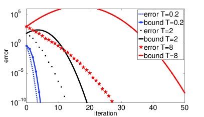
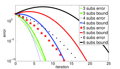
We show some experiments for the DNWR algorithm in the spatial domain $\Omega=(0,5)$, for the problem $\partial_{t}u=\Delta u,$ with initial condition $u_{0}(x)=x(5-x)$ and boundary conditions $u(0,t)=t^{2},u(5,t)=te^{-t}$. We discretize the heat equation using standard centered finite differences in space and backward Euler in time on a grid with $\Delta x=2\times 10^{-2}$ and $\Delta t=4\times 10^{-3}$. In the first experiment we apply the DNWR for a decomposition into five subdomains and for three different time windows $T=0.2,T=2$ and $T=8$, whereas for a fixed time $T=2$ we run another experiment for three to six equal subdomains. In Figure 9, on the left panel, we show the convergence estimates in the five-subdomain case as a function of time $T$, whereas on the right panel, we show the convergence for $T=2$ as we vary the number of subdomains. We observe superlinear convergence as predicted by Theorem 2, and for small $T$ the estimate is quite sharp. We also see that the convergence slows down as the number of subdomains is increased.

Fig. 9: Convergence estimates of DNWR for $\theta=1/2$, on the left for various values of $T$ for five subdomains, and on the right for various number of subdomains for $T=2$

Fig. 10: Arrangement A3: convergence of DNWR with various values of $\theta$ for $T=5$ on the left, and for various lengths $T$ of the time window and $\theta=1/2$ on the right

We now consider the following model wave equation to see the convergence behavior of the DNWR algorithm with multiple subdomains:

$$\partial_{tt}u =\partial_{xx}u, x\in(0,5),t>0,$$

$$u(x,0) =0,\>u_{t}(x,0)=0, 0<x<5,$$ (50)

$$u(0,t) =t^{2},\>u(5,t)=t^{2}e^{-t}, t>0,$$

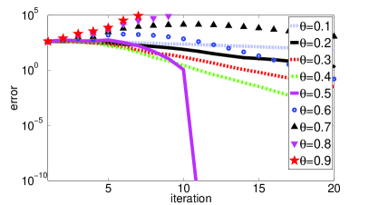
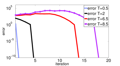
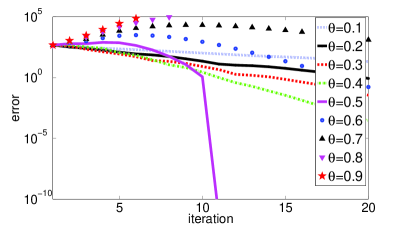
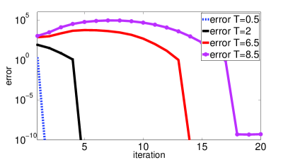
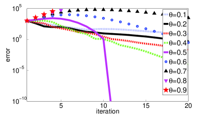
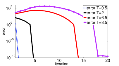
which is discretized using centered finite differences in both space and time on a grid with $\Delta x=\Delta t=2{\times}10^{-2}$. We take the initial guesses $g_{j}^{0}(t)=t^{2},t\in(0,T]$ for $1\leq j\leq 4$, and consider a decomposition of $(0,5)$ into five unequal subdomains, whose widths $h_{i}$ are $1,0.5,1.5,1,1$ respectively, so that $h_{\min}=0.5$. On the left panel of Figure 10, we show the convergence for different values of the parameter $\theta$ for $T=5$, and on the right panel the error curves for the best parameter $\theta=1/2$ for different time window length $T$. These convergence curves justify our convergence result for the arrangement A3 in Theorem 4. We observe two-step convergence for $\theta=1/2$ for a sufficiently small time window $T$. Coincidentally we observe exactly the same convergence behavior for other two corresponding arrangements A1 and A2 from Subsection 2.1, see Figure 11 and Figure 12 respectively.

Fig. 11: Arrangement A1: convergence of DNWR with various values of $\theta$ for $T=5$ on the left, and for various lengths $T$ of the time window and $\theta=1/2$ on the right

Fig. 12: Arrangement A2: convergence of DNWR with various values of $\theta$ for $T=5$ on the left, and for various lengths $T$ of the time window and $\theta=1/2$ on the right

Next we show an experiment for the DNWR algorithm in two dimension for the following model problem

$$\partial_{tt}u-\left(\partial_{xx}u+\partial_{yy}u\right)=0,u(x,y,0)=xy(x-1)(y-\pi)(5x-2)(4x-3),u_{t}(x,y,0)=0,$$

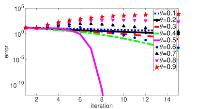
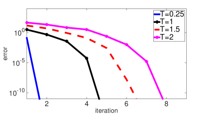
with homogeneous Dirichlet boundary conditions. We discretize the wave equation using the centered finite difference in both space and time (Leapfrog scheme) on a grid with $\Delta x=5{\times}10^{-2},\Delta y=16{\times}10^{-2},\Delta t=4{\times}10^{-2}$. We decompose our domain $\Omega:=(0,1)\times(0,\pi)$ into three non-overlapping subdomains $\Omega_{1}=(0,2/5)\times(0,\pi)$, $\Omega_{2}=(2/5,3/4)\times(0,\pi)$, $\Omega_{3}=(3/4,1)\times(0,\pi)$. As initial guesses, we take $w_{i}^{0}(y,t)=t\sin(y)$. In Figure 13 we plot the convergence curves for different values of the parameter $\theta$ for $T=2$ on the left panel, and on the right the results for the best parameter $\theta=1/2$ for different time window length $T$.

Fig. 13: Convergence of DNWR in 2D: curves for different values of $\theta$ for $T=2$ on the left, and for various time lengths $T$ and $\theta=1/2$ on the right

We now compare in Figure 14 the performance of the DNWR algorithm with its counterpart NNWR method [14, 9] and the SWR algorithms with and without overlap [7, 5]. Here we consider the model problem

$$\partial_{tt}u-\left(\partial_{xx}u+\partial_{yy}u\right)=0,u(x,y,0)=0=u_{t}(x,y,0),$$

with Dirichlet boundary conditions $u(0,y,t)=t^{2}\sin(y),u(1,y,t)=y(y-\pi)t^{3}$ and $u(x,0,t)=0=u(x,\pi,t)$. We decompose our domain $\Omega:=(0,1)\times(0,\pi)$ for the two subdomains experiment into $\Omega_{1}=(0,3/5)\times(0,\pi)$ and $\Omega_{2}=(3/5,1)\times(0,\pi)$, and for the three subdomains experiment into $\Omega_{1}=(0,2/5)\times(0,\pi)$, $\Omega_{2}=(2/5,3/4)\times(0,\pi)$, $\Omega_{3}=(3/4,1)\times(0,\pi)$. We take a random initial guess to start the iteration, and for the overlapping SWR we use an overlap of length $2\Delta x$ in all the experiments. We implement first order methods with one parameter in optimized SWR iterations; for more details see [5]. On the left panel of Figure 14 we plot the comparison curves for two subdomains, and the same for three subdomains on the right.

Fig. 14: Comparison of DNWR, NNWR, and SWR for $T=2$ in 2D for two subdomains on the left, and three subdomains on the right

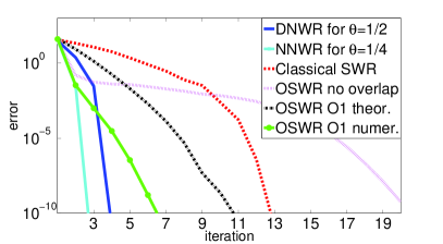
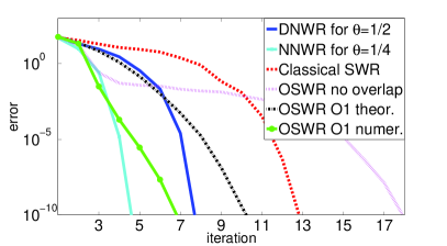
Here we consider a comparison of performances between the DNWR and the NNWR algorithms for the wave equation. Table 1 gives a summary of the theoretical results from Section 3 and 6 and [14, 9], to indicate the maximum number of iterations needed for the 1D and 2D wave equation to converge to the exact solution.

Table 1: Comparison of steps needed for convergence of DNWR and NNWR for the wave equation.

Methods	2 subdomains, 1D	Many subdomains, 1D	Many subdomains, 2D
DNWR	$T\leq 2kh_{\min}/c$	$T\leq kh_{\min}/c$	$T<kh_{\min}/c$
NNWR	$T\leq 4kh_{\min}/c$	$T\leq 2kh_{\min}/c$	$T<2kh_{\min}/c$

Table 2: Propagation speed and time steps for different subdomains.

	$\Omega_{1}$	$\Omega_{2}$	$\Omega_{3}$
wave speed $c$	$1/4$	$2$	$1/2$
time grids $\Delta t_{i}$	$13\times 10^{-2}$	$39\times 10^{-3}$	$1\times 10^{-1}$

Next we show a numerical experiment for the DNWR algorithm with different time grids for different subdomains and discontinuous wave speed across interfaces. We consider the model problem

$$\partial_{tt}u-c^{2}\partial_{xx}u=0,u(x,0)=0=u_{t}(x,0),$$

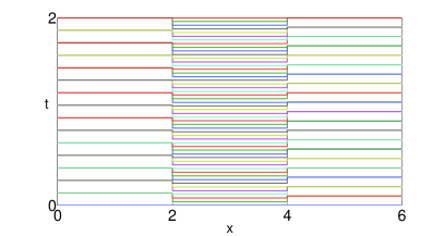
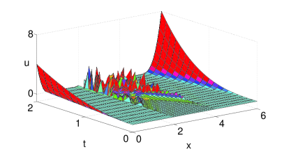
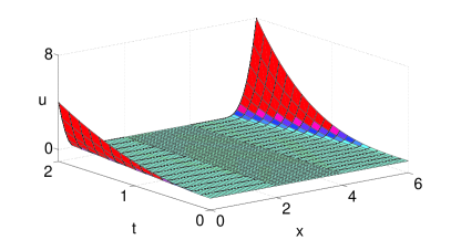
with Dirichlet boundary conditions $u(0,t)=t^{2},u(6,t)=t^{3}$. Suppose the spatial domain $\Omega:=(0,6)$ is decomposed into three equal subdomains $\Omega_{i},i=1,2,3$, and the random initial guesses are used to start the DNWR iteration. For the spatial discretization, we take a uniform mesh with size $\Delta x=1{\times}10^{-1}$, and for the time discretization, we use non-uniform time grids $\Delta t_{i},i=1,2,3$, as given in Table 2. For the non-uniform mesh grid, boundary data is transmitted from one subdomain to a neighboring subdomain by introducing a suitable time projection. For two dimensional problems, the interface is one dimensional. Using ideas of merge sort one can compute the projection with linear cost, see [8] and the references therein. In Figure 15(a) we show the non-uniform time steps for different subdomains. Figure 15(b), (c) and (d) give the three-step convergence of the DNWR algorithm for $T=2$.

(a) Non-uniform time-stepping

(b) DNWR: 1st iteration

(c) DNWR: 2nd iteration

(d) DNWR: 3rd iteration

Fig. 15: Convergence of the DNWR method applied to the wave equation for non-uniform time steps for $\theta=1/2$ for $T=2$

8 Conclusions

We defined the DNWR algorithm for multiple subdomains for parabolic and hyperbolic problems, and analyzed its convergence properties for one dimensional heat and wave equations. We proved using numerical experiments that for a particular choice of the relaxation parameter, $\theta=1/2$, superlinear convergence can be obtained for heat equation, whereas we showed finite step convergence for wave equation. In fact, the algorithm can be used as a two-step method for the wave equation, choosing the time window lengh $T$ small enough. We have also extended the DNWR algorithm for 2D wave equation, and analyzed its convergence properties. We have also shown using numerical experiments that among DNWR and NNWR, the second converges faster. But in comparison to DNWR, the NNWR has to solve twice the number of subproblems (once for Dirichlet subproblems, and once for Neumann subproblems) on each subdomain at each iteration. Therefore the computational cost is almost double for the NNWR than for the DNWR algorithm at each step. However, we get better convergence behavior with the NNWR in terms of iteration numbers. Finally we presented a comparison of performences between the DNWR, NNWR and Schwarz WR methods, and showed that the DNWR and NNWR converge faster than optimized SWR at least for higher dimensions.

References

- [1] P. E. Bjørstad and O. B. Widlund, Iterative Methods for the Solution of Elliptic Problems on Regions Partitioned into Substructures, SIAM J. Numer. Anal., (1986).
- [2] J. F. Bourgat, R. Glowinski, P. L. Tallec, and M. Vidrascu, Variational Formulation and Algorithm for Trace Operator in Domain Decomposition Calculations, in Domain Decomposition Methods, T. F. Chan, R. Glowinski, J. Périaux, and O. B. Widlund, eds., SIAM, 1989, pp. 3–16.
- [3] J. H. Bramble, J. E. Pasciak, and A. H. Schatz, An Iterative Method for Elliptic Problems on Regions Partitioned into Substructures, Mathematics of Computation, (1986).
- [4] D. Funaro, A. Quarteroni, and P. Zanolli, An Iterative Procedure with Interface Relaxation for Domain Decomposition Methods, SIAM J. Numer. Anal., 25 (1988), pp. 1213–1236.
- [5] M. J. Gander and L. Halpern, Absorbing Boundary Conditions for the Wave Equation and Parallel Computing, Math. of Comput., 74 (2004), pp. 153–176.
- [6] , Optimized Schwarz Waveform Relaxation for Advection Reaction Diffusion Problems, SIAM J. Num. Anal., 45 (2007), pp. 666–697.
- [7] M. J. Gander, L. Halpern, and F. Nataf, Optimal Schwarz Waveform Relaxation for the One Dimensional Wave Equation, SIAM J. Num. Anal., 41 (2003), pp. 1643–1681.
- [8] M. J. Gander and C. Japhet, An Algorithm for Non-Matching Grid Projections with Linear Complexity, in Domain Decomposition in Science and Engineering XVIII, M. Bercovier, M. J. Gander, D. Keyes, and O. Widlund, eds., 2008.
- [9] M. J. Gander, F. Kwok, and B. C. Mandal, Dirichlet-Neumann and Neumann-Neumann Waveform Relaxation for the Wave Equation, in Domain Decomposition in Science and Engineering XXII, Springer-Verlag, 2015.
- [10] , Dirichlet-Neumann and Neumann-Neumann Waveform Relaxation Algorithms for Parabolic Problems, submitted, (arXiv:1311.2709).
- [11] M. J. Gander and A. M. Stuart, Space-time continuous analysis of waveform relaxation for the heat equation, SIAM J. for Sci. Comput., 19 (1998), pp. 2014–2031.
- [12] E. Giladi and H. Keller, Space time domain decomposition for parabolic problems, Tech. Report 97-4, Center for research on parallel computation CRPC, Caltech, 1997.
- [13] F. Kwok, Neumann-Neumann Waveform Relaxation for the Time-Dependent Heat Equation, in Domain Decomposition in Science and Engineering XXI, J. Erhel, M. J. Gander, L. Halpern, G. Pichot, T. Sassi, and O. B. Widlund, eds., vol. 98, Springer-Verlag, 2014, pp. 189–198.
- [14] B. C. Mandal, Neumann-Neumann Waveform Relaxation Algorithm in Multiple Subdomains for Hyperbolic Problems in 1d and 2d, in Preparation.
- [15] , Convergence Analysis of Substructuring Waveform Relaxation Methods for Space-time Problems and Their Application to Optimal Control Problems, 2014. Thesis (Ph.D.)–University of Geneva.
- [16] , A Time-Dependent Dirichlet-Neumann Method for the Heat Equation, in Domain Decomposition in Science and Engineering XXI, J. Erhel, M. J. Gander, L. Halpern, G. Pichot, T. Sassi, and O. B. Widlund, eds., vol. 98, Springer-Verlag, 2014, pp. 467–475.
- [17] L. Martini and A. Quarteroni, An Iterative Procedure for Domain Decomposition Methods: a Finite Element Approach, SIAM, in Domain Decomposition Methods for PDEs, I, (1988), pp. 129–143.
- [18] , A Relaxation Procedure for Domain Decomposition Method using Finite Elements, Numer. Math., (1989).
- [19] Fritz Oberhettinger and L. Badii, Tables of Laplace Transforms, Springer-Verlag, 1973.
- [20] Y. D. Roeck and P. L. Tallec, Analysis and Test of a local domain decomposition preconditioner, in Domain Decomposition Methods for PDEs, I, R. Glowinski et al., ed., Philadelphia, 1991, SIAM, pp. 112–128.
- [21] J. L. Schiff, The Laplace Transform, Springer, 1991.
- [22] P. L. Tallec, Y. D. Roeck, and M. Vidrascu, Domain decomposition methods for large linearly elliptic three-dimensional problems, J. of Comput. and App. Math., (1991).
- [23] A. Toselli and O. B. Widlund, Domain Decomposition Methods, Algorithms and Theory, Springer, 2005.