Neumann-Neumann Waveform Relaxation Algorithm in Multiple subdomains for Hyperbolic Problems in 1D and 2D

Bankim C. Mandal Department of Mathematical Sciences, Michigan Technological University, USA (bmandal@mtu.edu).
Abstract

We present a Waveform Relaxation (WR) version of the Neumann-Neumann algorithm for the wave equation in space-time. The method is based on a non-overlapping spatial domain decomposition, and the iteration involves subdomain solves in space-time with corresponding interface condition, followed by a correction step. Using a Fourier-Laplace transform argument, for a particular relaxation parameter, we prove convergence of the algorithm in a finite number of steps for finite time intervals. The number of steps depends on the size of the subdomains and the time window length on which the algorithm is employed. We illustrate the performance of the algorithm with numerical results, followed by a comparison with classical and optimized Schwarz WR methods.

keywords:
Neumann-Neumann, Waveform Relaxation, Wave equation, Domain Decomposition.

1 Introduction

We formulate a new variant of Waveform Relaxation (WR) methods based on the Neumann-Neumann algorithm to solve hyperbolic problems in parallel computer, and present convergence results for the method. The Neumann-Neumann algorithm was introduced for solving elliptic problems by Bourgat et al. [1], see also [26] and [28]. The iteration involves solving the subdomain problems using Dirichlet interface conditions in the first step, followed by a correction step involving Neumann interface conditions. The convergence behavior of the algorithm is now well understood for elliptic problems, see for example the book [29].

To solve time-dependent problems in parallel, the following three possible classes of domain decomposition techniques exist:

  • this approach consists of discretizing the problem uniformly in time with an implicit scheme to obtain a sequence of elliptic problems, which are then solved by DD methods. For this kind of technique, we refer to [2, 3]. One disadvantage of this approach is that, uniform time step across the whole domain need to be enforced, which is very restrictive for problems with variable coefficients or multiple time scales. Also this method is expensive for parallel computation, since one needs to exchange information at each time step of the discretization.

  • in this approach the equation is first discretized in space, which is called the method of lines, and then one applies a waveform relaxation algorithm to solve the large system of ordinary differential equations (ODEs) obtained from the space-discretization process. Multigrid dynamic iteration [21, 16] and multi-splitting algorithms [17] are some particular examples of this approach.

  • in contrast to the two classical techniques above, there exist space-time domain decomposition methods, formulated at the continuous level. Here, instead of discretizing in time or in space, one decomposes the original spatial domain into smaller subdomains and considers each subproblem as posed in both space and time; then the subproblems are solved iteratively communicating information at the interfaces between subdomains. This permits the use of different numerical methods in different subdomains. At each iteration, one solves the space-time subproblem over the entire time interval of interest, before communicating interface data across subdomains. Thus one saves communication time while computing in parallel computer. For this approach, see [14, 15, 4, 6, 24] for parabolic problems, and [8, 5, 7] for hyperbolic problems.

In this article, we focus on the WR-type algorithm as it allows different discretizations in different space-time subdomains. WR methods have their origin in the work of Picard [25] and Lindelöf [20] in the late 19th century. Lelarasmee, Ruehli and Sangiovanni-Vincentelli [19] rediscovered WR as a parallel method for the solution of ODEs.

In a different viewpoint, the WR-type methods can be seen as an extension of DD methods for elliptic PDEs. The systematic extension of the classical Schwarz method to time-dependent parabolic problems was started in [14, 15]; later optimized SWR methods have been introduced to achieve faster convergence or convergence with no overlap, see [6] for parabolic problems, and [8] for hyperbolic problems. Recently, we extended the substructuring methods, namely the Dirichlet-Neumann and Neumann-Neumann methods, to space-time problems; for parabolic problems see [13, 23, 18, 11, 22], and for hyperbolic problems see [12, 11, 22]. We analyzed for the heat equation to prove that on finite time intervals, the Dirichlet-Neumann Waveform Relaxation (DNWR) and the Neumann-Neumann Waveform Relaxation (NNWR) methods converge superlinearly for an optimal choice of the relaxation parameter. On the contrary for the wave equation, these methods with a two-subdomains decomposition converge in a finite no of steps, see [11]. In this paper, we propose the NNWR method with many subdomains decomposition for hyperbolic problems and analyze the method for the Wave equation in one and two space dimensions. We analyze the method in the continuous setting to ensure the understanding of the asymptotic behavior of the methods in the case of fine grids.

We consider the following hyperbolic PDE on a bounded domain Ωd,0<t<Tformulae-sequenceΩsuperscript𝑑0𝑡𝑇\Omega\subset\mathbb{R}^{d},0<t<T, d=1,2,3𝑑123d=1,2,3, with a smooth boundary as our guiding example,

2ut2c2(𝒙)Δu=f(𝒙,t),𝒙Ω,0<t<T,u(𝒙,0)=u0(𝒙),𝒙Ω,ut(𝒙,0)=v0(𝒙),𝒙Ω,u(𝒙,t)=g(𝒙,t),𝒙Ω,0<t<T,superscript2𝑢superscript𝑡2superscript𝑐2𝒙Δ𝑢𝑓𝒙𝑡formulae-sequence𝒙Ω0𝑡𝑇𝑢𝒙0subscript𝑢0𝒙𝒙Ωsubscript𝑢𝑡𝒙0subscript𝑣0𝒙𝒙Ω𝑢𝒙𝑡𝑔𝒙𝑡formulae-sequence𝒙Ω0𝑡𝑇\begin{array}[]{rcll}\frac{\partial^{2}u}{\partial t^{2}}-c^{2}(\boldsymbol{x})\Delta u&=&f(\boldsymbol{x},t),&\boldsymbol{x}\in\Omega,0<t<T,\\ u(\boldsymbol{x},0)&=&u_{0}(\boldsymbol{x}),&\boldsymbol{x}\in\Omega,\\ u_{t}(\boldsymbol{x},0)&=&v_{0}(\boldsymbol{x}),&\boldsymbol{x}\in\Omega,\\ u(\boldsymbol{x},t)&=&g(\boldsymbol{x},t),&\boldsymbol{x}\in\partial\Omega,0<t<T,\end{array} (1)

with c(𝒙)𝑐𝒙c(\boldsymbol{x}) being a positive function.

We introduce in Section 2 the non-overlapping NNWR algorithm with multiple subdomains for the model problem (1), and then analyze its convergence for the one dimensional wave equation. In Section 3 we present convergence result of the NNWR for multiple subdomains in 2D. Our convergence analysis shows that both the NNWR algorithm converge in a finite no of steps for finite time intervals, T<𝑇T<\infty. Finally we present numerical results in Section 4, which illustrate our analysis.

2 NNWR for multiple subdomains

In this section we define the Neumann-Neumann Waveform Relaxation (NNWR) method with many subdomains for the model problem (1) on the space-time domain Ω×(0,T)Ω0𝑇\Omega\times(0,T) with Dirichlet data given on ΩΩ\partial\Omega. This can be treated as a generalization of the NNWR algorithm for two subdomains, for which see [12]. The method starts with a non-overlapping spatial domain decomposition, and the iteration involves subdomain solves in space time with corresponding interface condition, followed by a correction step.

2.1 NNWR algorithm

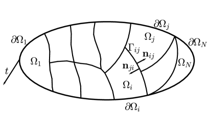
Suppose the spatial domain ΩΩ\Omega is partitioned into N𝑁N non-overlapping subdomains {Ωi\{\Omega_{i}, 1iN}1\leq i\leq N\}, as illustrated in the left panel of Figure 1. For i=1,,N𝑖1𝑁i=1,\ldots,N set Γi:=ΩiΩassignsubscriptΓ𝑖subscriptΩ𝑖Ω\Gamma_{i}:=\partial\Omega_{i}\setminus\partial\Omega, Λi:={j{1,,N}:ΓiΓjhas nonzero measure}assignsubscriptΛ𝑖conditional-set𝑗1𝑁subscriptΓ𝑖subscriptΓ𝑗has nonzero measure\Lambda_{i}:=\{j\in\{1,\ldots,N\}:\Gamma_{i}\cap\Gamma_{j}\,\mbox{has nonzero measure}\} and Γij:=ΩiΩjassignsubscriptΓ𝑖𝑗subscriptΩ𝑖subscriptΩ𝑗\Gamma_{ij}:=\partial\Omega_{i}\cap\partial\Omega_{j}, so that the interface of ΩisubscriptΩ𝑖\Omega_{i} can be rewritten as Γi=jΛiΓijsubscriptΓ𝑖subscript𝑗subscriptΛ𝑖subscriptΓ𝑖𝑗\Gamma_{i}=\bigcup_{j\in\Lambda_{i}}\Gamma_{ij}. We denote by uisubscript𝑢𝑖u_{i} the restriction of the solution u𝑢u of (1) to ΩisubscriptΩ𝑖\Omega_{i} and by 𝒏ijsubscript𝒏𝑖𝑗\boldsymbol{n}_{ij} the unit outward normal for ΩisubscriptΩ𝑖\Omega_{i} on the interface ΓijsubscriptΓ𝑖𝑗\Gamma_{ij}. The NNWR algorithm for the model problem (1) starts with an initial guess wij0(𝒙,t)superscriptsubscript𝑤𝑖𝑗0𝒙𝑡w_{ij}^{0}(\boldsymbol{x},t) along the interfaces Γij×(0,T)subscriptΓ𝑖𝑗0𝑇\Gamma_{ij}\times(0,T), jΛi𝑗subscriptΛ𝑖j\in\Lambda_{i}, i=1,,N𝑖1𝑁i=1,\ldots,N, and then performs the following two-step iteration: one first solves Dirichlet subproblems on each ΩisubscriptΩ𝑖\Omega_{i} in parallel,

ttuikc2(𝒙)Δuik=f,in Ωi,uik(𝒙,0)=u0(𝒙),in Ωi,tuik(𝒙,0)=v0(𝒙),in Ωi,uik=g,on ΩiΓi,uik=wijk1,on Γij,jΛi.subscript𝑡𝑡superscriptsubscript𝑢𝑖𝑘superscript𝑐2𝒙Δsuperscriptsubscript𝑢𝑖𝑘𝑓in Ωisuperscriptsubscript𝑢𝑖𝑘𝒙0subscript𝑢0𝒙in Ωisubscript𝑡superscriptsubscript𝑢𝑖𝑘𝒙0subscript𝑣0𝒙in Ωisuperscriptsubscript𝑢𝑖𝑘𝑔on ΩiΓisuperscriptsubscript𝑢𝑖𝑘superscriptsubscript𝑤𝑖𝑗𝑘1on Γij,jΛi\begin{array}[]{rcll}\partial_{tt}u_{i}^{k}-c^{2}(\boldsymbol{x})\Delta u_{i}^{k}&=&f,&\mbox{in $\Omega_{i}$},\\ u_{i}^{k}(\boldsymbol{x},0)&=&u_{0}(\boldsymbol{x}),&\mbox{in $\Omega_{i}$},\\ \partial_{t}u_{i}^{k}(\boldsymbol{x},0)&=&v_{0}(\boldsymbol{x}),&\mbox{in $\Omega_{i}$},\\ u_{i}^{k}&=&g,&\mbox{on $\partial\Omega_{i}\setminus\Gamma_{i}$},\\ u_{i}^{k}&=&w_{ij}^{k-1},&\mbox{on $\Gamma_{ij},j\in\Lambda_{i}$}.\end{array} (2)

One then solves Neumann subproblems on all subdomains,

ttφikc2(𝒙)Δφik=0,in Ωi,φik(𝒙,0)=0,in Ωi,tφik(𝒙,0)=0,in Ωi,φik=0,on ΩiΓi,𝒏ijφik=𝒏ijuik+𝒏jiujk,on Γij,jΛi.subscript𝑡𝑡superscriptsubscript𝜑𝑖𝑘superscript𝑐2𝒙Δsuperscriptsubscript𝜑𝑖𝑘0in Ωisuperscriptsubscript𝜑𝑖𝑘𝒙00in Ωisubscript𝑡superscriptsubscript𝜑𝑖𝑘𝒙00in Ωisuperscriptsubscript𝜑𝑖𝑘0on ΩiΓisubscriptsubscript𝒏𝑖𝑗superscriptsubscript𝜑𝑖𝑘subscriptsubscript𝒏𝑖𝑗superscriptsubscript𝑢𝑖𝑘subscriptsubscript𝒏𝑗𝑖superscriptsubscript𝑢𝑗𝑘on Γij,jΛi\begin{array}[]{rcll}\partial_{tt}\varphi_{i}^{k}-c^{2}(\boldsymbol{x})\Delta\varphi_{i}^{k}&=&0,&\mbox{in $\Omega_{i}$},\\ \varphi_{i}^{k}(\boldsymbol{x},0)&=&0,&\mbox{in $\Omega_{i}$},\\ \partial_{t}\varphi_{i}^{k}(\boldsymbol{x},0)&=&0,&\mbox{in $\Omega_{i}$},\\ \varphi_{i}^{k}&=&0,&\mbox{on $\partial\Omega_{i}\setminus\Gamma_{i}$},\\ \partial_{\boldsymbol{n}_{ij}}\varphi_{i}^{k}&=&\partial_{\boldsymbol{n}_{ij}}u_{i}^{k}+\partial_{\boldsymbol{n}_{ji}}u_{j}^{k},&\mbox{on $\Gamma_{ij},j\in\Lambda_{i}$}.\end{array} (3)

with the updating condition

wijk(𝒙,t)=wijk1(𝒙,t)θ(φik|+Γij×(0,T)φjk|)Γij×(0,T),w_{ij}^{k}(\boldsymbol{x},t)=w_{ij}^{k-1}(\boldsymbol{x},t)-\theta\left(\varphi_{i}^{k}\left|{}_{\Gamma_{ij}\times(0,T)}\right.+\varphi_{j}^{k}\left|{}_{\Gamma_{ij}\times(0,T)}\right.\right), (4)

where θ(0,1]𝜃01\theta\in(0,1] is a relaxation parameter.

Refer to caption
Refer to caption
Fig. 1: Splitting into many non-overlapping subdomains

2.2 Convergence analysis for 1D

We prove our convergence result for the one dimensional wave equation with constant speed, c(x)=c𝑐𝑥𝑐c(x)=c on the domain Ω:=(0,L)assignΩ0𝐿\Omega:=(0,L) with boundary conditions u(0,t)=g0(t)𝑢0𝑡subscript𝑔0𝑡u(0,t)=g_{0}(t) and u(L,t)=gL(t)𝑢𝐿𝑡subscript𝑔𝐿𝑡u(L,t)=g_{L}(t), which in turn become zeros as we consider the error equations, f(x,t)=0,g0(t)=gL(t)=0=u0(x)=v0(x)formulae-sequence𝑓𝑥𝑡0subscript𝑔0𝑡subscript𝑔𝐿𝑡0subscript𝑢0𝑥subscript𝑣0𝑥f(x,t)=0,g_{0}(t)=g_{L}(t)=0=u_{0}(x)=v_{0}(x). We decompose ΩΩ\Omega into non-overlapping subdomains Ωi:=(xi1,xi)assignsubscriptΩ𝑖subscript𝑥𝑖1subscript𝑥𝑖\Omega_{i}:=(x_{i-1},x_{i}), i=1,,N𝑖1𝑁i=1,\ldots,N, as shown in the right panel of Figure 1, and define the subdomain length hi:=xixi1assignsubscript𝑖subscript𝑥𝑖subscript𝑥𝑖1h_{i}:=x_{i}-x_{i-1}, and hmin:=min1iNhiassignsubscriptsubscript1𝑖𝑁subscript𝑖h_{\min}:=\min_{1\leq i\leq N}h_{i}. Our initial guess is denoted by {wi0(t)}i=1N1superscriptsubscriptsuperscriptsubscript𝑤𝑖0𝑡𝑖1𝑁1\left\{w_{i}^{0}(t)\right\}_{i=1}^{N-1} on the interfaces {x=xi}×(0,T)𝑥subscript𝑥𝑖0𝑇\left\{x=x_{i}\right\}\times(0,T), and for sake of consistency we denote w0k(t)=wNk(t)=0superscriptsubscript𝑤0𝑘𝑡superscriptsubscript𝑤𝑁𝑘𝑡0w_{0}^{k}(t)=w_{N}^{k}(t)=0 for all k𝑘k. We then obtain

ttuikc2xxuik=0,in Ωi,ttφikc2xxφik=0,in Ωi,uik(x,0)=0,in Ωi,φik(x,0)=0,in Ωi,tuik(x,0)=0,in Ωi,tφik(x,0)=0,in Ωi,uik(xi1,t)=wi1k1(t),xφik(xi1,t)=(xui1kxuik)(xi1,t),uik(xi,t)=wik1(t),xφik(xi,t)=(xuikxui+1k)(xi,t),subscript𝑡𝑡superscriptsubscript𝑢𝑖𝑘superscript𝑐2subscript𝑥𝑥superscriptsubscript𝑢𝑖𝑘0in Ωisubscript𝑡𝑡superscriptsubscript𝜑𝑖𝑘superscript𝑐2subscript𝑥𝑥superscriptsubscript𝜑𝑖𝑘0in Ωisuperscriptsubscript𝑢𝑖𝑘𝑥00in Ωisuperscriptsubscript𝜑𝑖𝑘𝑥00in Ωisubscript𝑡superscriptsubscript𝑢𝑖𝑘𝑥00in Ωisubscript𝑡superscriptsubscript𝜑𝑖𝑘𝑥00in Ωisuperscriptsubscript𝑢𝑖𝑘subscript𝑥𝑖1𝑡superscriptsubscript𝑤𝑖1𝑘1𝑡subscript𝑥superscriptsubscript𝜑𝑖𝑘subscript𝑥𝑖1𝑡subscript𝑥superscriptsubscript𝑢𝑖1𝑘subscript𝑥superscriptsubscript𝑢𝑖𝑘subscript𝑥𝑖1𝑡superscriptsubscript𝑢𝑖𝑘subscript𝑥𝑖𝑡superscriptsubscript𝑤𝑖𝑘1𝑡subscript𝑥superscriptsubscript𝜑𝑖𝑘subscript𝑥𝑖𝑡subscript𝑥superscriptsubscript𝑢𝑖𝑘subscript𝑥superscriptsubscript𝑢𝑖1𝑘subscript𝑥𝑖𝑡\begin{array}[]{rclrcl}\partial_{tt}u_{i}^{k}-c^{2}\partial_{xx}u_{i}^{k}&=&0,\qquad\textrm{in $\Omega_{i}$},&\partial_{tt}\varphi_{i}^{k}-c^{2}\partial_{xx}\varphi_{i}^{k}&=&0,\qquad\textrm{in $\Omega_{i}$},\\ u_{i}^{k}(x,0)&=&0,\qquad\textrm{in $\Omega_{i}$},&\varphi_{i}^{k}(x,0)&=&0,\qquad\textrm{in $\Omega_{i}$},\\ \partial_{t}u_{i}^{k}(x,0)&=&0,\qquad\textrm{in $\Omega_{i}$},&\partial_{t}\varphi_{i}^{k}(x,0)&=&0,\qquad\textrm{in $\Omega_{i}$},\\ u_{i}^{k}(x_{i-1},t)&=&w_{i-1}^{k-1}(t),&-\partial_{x}\varphi_{i}^{k}(x_{i-1},t)&=&(\partial_{x}u_{i-1}^{k}-\partial_{x}u_{i}^{k})(x_{i-1},t),\\ u_{i}^{k}(x_{i},t)&=&w_{i}^{k-1}(t),&\partial_{x}\varphi_{i}^{k}(x_{i},t)&=&(\partial_{x}u_{i}^{k}-\partial_{x}u_{i+1}^{k})(x_{i},t),\end{array} (5)

except for the first and last subdomains, where the Neumann conditions in the Neumann step are replaced by homogeneous Dirichlet conditions along the physical boundaries. The updated interface values for the next step will be

wik(t)=wik1(t)θ(φik(xi,t)+φi+1k(xi,t)).superscriptsubscript𝑤𝑖𝑘𝑡superscriptsubscript𝑤𝑖𝑘1𝑡𝜃superscriptsubscript𝜑𝑖𝑘subscript𝑥𝑖𝑡superscriptsubscript𝜑𝑖1𝑘subscript𝑥𝑖𝑡w_{i}^{k}(t)=w_{i}^{k-1}(t)-\theta\left(\varphi_{i}^{k}(x_{i},t)+\varphi_{i+1}^{k}(x_{i},t)\right). (6)

We start by applying the Laplace transform to the homogeneous Dirichlet subproblems in (5), and obtain

s2u^ic2u^i,xx=0,u^i(xi1,s)=w^i1(s),u^i(xi,s)=w^i(s),formulae-sequencesuperscript𝑠2subscript^𝑢𝑖superscript𝑐2subscript^𝑢𝑖𝑥𝑥0formulae-sequencesubscript^𝑢𝑖subscript𝑥𝑖1𝑠subscript^𝑤𝑖1𝑠subscript^𝑢𝑖subscript𝑥𝑖𝑠subscript^𝑤𝑖𝑠s^{2}\hat{u}_{i}-c^{2}\hat{u}_{i,xx}=0,\quad\hat{u}_{i}(x_{i-1},s)=\hat{w}_{i-1}(s),\quad\hat{u}_{i}(x_{i},s)=\hat{w}_{i}(s),

for i=2,,N1.𝑖2𝑁1i=2,...,N-1. Set γi=cosh(his/c),σi=sinh(his/c).formulae-sequencesubscript𝛾𝑖subscript𝑖𝑠𝑐subscript𝜎𝑖subscript𝑖𝑠𝑐\gamma_{i}=\cosh\left(h_{i}s/c\right),\sigma_{i}=\sinh\left(h_{i}s/c\right). These subdomain problems have the solutions

u^i(x,s)=1σi(w^i(s)sinh((xxi1)s/c)+w^i1(s)sinh((xix)s/c)).subscript^𝑢𝑖𝑥𝑠1subscript𝜎𝑖subscript^𝑤𝑖𝑠𝑥subscript𝑥𝑖1𝑠𝑐subscript^𝑤𝑖1𝑠subscript𝑥𝑖𝑥𝑠𝑐\hat{u}_{i}(x,s)=\frac{1}{\sigma_{i}}\left(\hat{w}_{i}(s)\sinh\left((x-x_{i-1})s/c\right)+\hat{w}_{i-1}(s)\sinh\left((x_{i}-x)s/c\right)\right).

Next we apply the Laplace transform to the Neumann subproblems in (5) for subdomains not touching the physical boundary, and obtain

φ^i(x,s)=Ci(s)cosh((xxi1)s/c)+Di(s)cosh((xix)s/c),subscript^𝜑𝑖𝑥𝑠subscript𝐶𝑖𝑠𝑥subscript𝑥𝑖1𝑠𝑐subscript𝐷𝑖𝑠subscript𝑥𝑖𝑥𝑠𝑐\hat{\varphi}_{i}(x,s)=C_{i}(s)\cosh\left((x-x_{i-1})s/c\right)+D_{i}(s)\cosh\left((x_{i}-x)s/c\right),

where

Cisubscript𝐶𝑖\displaystyle C_{i} =\displaystyle= 1σi(w^i(γiσi+γi+1σi+1)w^i1σiw^i+1σi+1),1subscript𝜎𝑖subscript^𝑤𝑖subscript𝛾𝑖subscript𝜎𝑖subscript𝛾𝑖1subscript𝜎𝑖1subscript^𝑤𝑖1subscript𝜎𝑖subscript^𝑤𝑖1subscript𝜎𝑖1\displaystyle\frac{1}{\sigma_{i}}\left(\hat{w}_{i}\left(\frac{\gamma_{i}}{\sigma_{i}}+\frac{\gamma_{i+1}}{\sigma_{i+1}}\right)-\frac{\hat{w}_{i-1}}{\sigma_{i}}-\frac{\hat{w}_{i+1}}{\sigma_{i+1}}\right),
Disubscript𝐷𝑖\displaystyle D_{i} =\displaystyle= 1σi(w^i1(γiσi+γi1σi1)w^i2σi1w^iσi).1subscript𝜎𝑖subscript^𝑤𝑖1subscript𝛾𝑖subscript𝜎𝑖subscript𝛾𝑖1subscript𝜎𝑖1subscript^𝑤𝑖2subscript𝜎𝑖1subscript^𝑤𝑖subscript𝜎𝑖\displaystyle\frac{1}{\sigma_{i}}\left(\hat{w}_{i-1}\left(\frac{\gamma_{i}}{\sigma_{i}}+\frac{\gamma_{i-1}}{\sigma_{i-1}}\right)-\frac{\hat{w}_{i-2}}{\sigma_{i-1}}-\frac{\hat{w}_{i}}{\sigma_{i}}\right).

We therefore obtain for i=2,,N2,𝑖2𝑁2i=2,...,N-2, at iteration k𝑘k

w^ik(s)superscriptsubscript^𝑤𝑖𝑘𝑠\displaystyle\hat{w}_{i}^{k}(s) =\displaystyle= w^ik1(s)θ(φ^ik(xi,s)+φ^i+1k(xi,s))superscriptsubscript^𝑤𝑖𝑘1𝑠𝜃superscriptsubscript^𝜑𝑖𝑘subscript𝑥𝑖𝑠superscriptsubscript^𝜑𝑖1𝑘subscript𝑥𝑖𝑠\displaystyle\hat{w}_{i}^{k-1}(s)-\theta\left(\hat{\varphi}_{i}^{k}(x_{i},s)+\hat{\varphi}_{i+1}^{k}(x_{i},s)\right)
=\displaystyle= w^ik1(s)θ(Ciγi+Di+Ci+1+Di+1γi+1).superscriptsubscript^𝑤𝑖𝑘1𝑠𝜃subscript𝐶𝑖subscript𝛾𝑖subscript𝐷𝑖subscript𝐶𝑖1subscript𝐷𝑖1subscript𝛾𝑖1\displaystyle\hat{w}_{i}^{k-1}(s)-\theta\left(C_{i}\gamma_{i}+D_{i}+C_{i+1}+D_{i+1}\gamma_{i+1}\right).

Using the identity γi21=σi2superscriptsubscript𝛾𝑖21superscriptsubscript𝜎𝑖2\gamma_{i}^{2}-1=\sigma_{i}^{2} and simplifying, we get

w^ik=w^ik1θ(w^ik1(2+2γiγi+1σiσi+1)+w^i+1k1σi+1(γi+2σi+2γiσi)+w^i1k1σi(γi1σi1γi+1σi+1)w^i+2k1σi+1σi+2w^i2k1σiσi1).superscriptsubscript^𝑤𝑖𝑘superscriptsubscript^𝑤𝑖𝑘1𝜃superscriptsubscript^𝑤𝑖𝑘122subscript𝛾𝑖subscript𝛾𝑖1subscript𝜎𝑖subscript𝜎𝑖1superscriptsubscript^𝑤𝑖1𝑘1subscript𝜎𝑖1subscript𝛾𝑖2subscript𝜎𝑖2subscript𝛾𝑖subscript𝜎𝑖superscriptsubscript^𝑤𝑖1𝑘1subscript𝜎𝑖subscript𝛾𝑖1subscript𝜎𝑖1subscript𝛾𝑖1subscript𝜎𝑖1superscriptsubscript^𝑤𝑖2𝑘1subscript𝜎𝑖1subscript𝜎𝑖2superscriptsubscript^𝑤𝑖2𝑘1subscript𝜎𝑖subscript𝜎𝑖1\hat{w}_{i}^{k}={\displaystyle\hat{w}_{i}^{k-1}-\theta\left(\hat{w}_{i}^{k-1}\left(2+\frac{2\gamma_{i}\gamma_{i+1}}{\sigma_{i}\sigma_{i+1}}\right)+\frac{\hat{w}_{i+1}^{k-1}}{\sigma_{i+1}}\left(\frac{\gamma_{i+2}}{\sigma_{i+2}}-\frac{\gamma_{i}}{\sigma_{i}}\right)\right.}\\ \left.+\frac{\hat{w}_{i-1}^{k-1}}{\sigma_{i}}\left(\frac{\gamma_{i-1}}{\sigma_{i-1}}-\frac{\gamma_{i+1}}{\sigma_{i+1}}\right)-\frac{\hat{w}_{i+2}^{k-1}}{\sigma_{i+1}\sigma_{i+2}}-\frac{\hat{w}_{i-2}^{k-1}}{\sigma_{i}\sigma_{i-1}}\right). (7)

For i=1𝑖1i=1 and i=N𝑖𝑁i=N, the Neumann conditions on the physical boundary are replaced by homogeneous Dirichlet conditions φ1(0,t)=0subscript𝜑10𝑡0\varphi_{1}(0,t)=0 and φN(L,t)=0subscript𝜑𝑁𝐿𝑡0\varphi_{N}(L,t)=0, t>0𝑡0t>0. For these two subdomains, we obtain as solution after a Laplace transform

φ^1(x,s)subscript^𝜑1𝑥𝑠\displaystyle\hat{\varphi}_{1}(x,s) =\displaystyle= 1γ1(w^1(γ1σ1+γ2σ2)w^2σ2)sinh((xx0)s/c),1subscript𝛾1subscript^𝑤1subscript𝛾1subscript𝜎1subscript𝛾2subscript𝜎2subscript^𝑤2subscript𝜎2𝑥subscript𝑥0𝑠𝑐\displaystyle\frac{1}{\gamma_{1}}\left(\hat{w}_{1}\left(\frac{\gamma_{1}}{\sigma_{1}}+\frac{\gamma_{2}}{\sigma_{2}}\right)-\frac{\hat{w}_{2}}{\sigma_{2}}\right)\sinh\left((x-x_{0})s/c\right),
φ^N(x,s)subscript^𝜑𝑁𝑥𝑠\displaystyle\hat{\varphi}_{N}(x,s) =\displaystyle= 1γN(w^N1(γN1σN1+γNσN)w^N2σN1)sinh((xNx)s/c),1subscript𝛾𝑁subscript^𝑤𝑁1subscript𝛾𝑁1subscript𝜎𝑁1subscript𝛾𝑁subscript𝜎𝑁subscript^𝑤𝑁2subscript𝜎𝑁1subscript𝑥𝑁𝑥𝑠𝑐\displaystyle\frac{1}{\gamma_{N}}\left(\hat{w}_{N-1}\left(\frac{\gamma_{N-1}}{\sigma_{N-1}}+\frac{\gamma_{N}}{\sigma_{N}}\right)-\frac{\hat{w}_{N-2}}{\sigma_{N-1}}\right)\sinh\left((x_{N}-x)s/c\right),

and thus the recurrence relations on the first interface is

w^1k=w^1k1θ(w^1k1(2+γ1γ2σ1σ2+σ1γ2γ1σ2)+w^2k1σ2(γ3σ3σ1γ1)w^3k1σ2σ3),superscriptsubscript^𝑤1𝑘superscriptsubscript^𝑤1𝑘1𝜃superscriptsubscript^𝑤1𝑘12subscript𝛾1subscript𝛾2subscript𝜎1subscript𝜎2subscript𝜎1subscript𝛾2subscript𝛾1subscript𝜎2superscriptsubscript^𝑤2𝑘1subscript𝜎2subscript𝛾3subscript𝜎3subscript𝜎1subscript𝛾1superscriptsubscript^𝑤3𝑘1subscript𝜎2subscript𝜎3\hat{w}_{1}^{k}=\hat{w}_{1}^{k-1}-\theta\left(\hat{w}_{1}^{k-1}\left(2+\frac{\gamma_{1}\gamma_{2}}{\sigma_{1}\sigma_{2}}+\frac{\sigma_{1}\gamma_{2}}{\gamma_{1}\sigma_{2}}\right)+\frac{\hat{w}_{2}^{k-1}}{\sigma_{2}}\left(\frac{\gamma_{3}}{\sigma_{3}}-\frac{\sigma_{1}}{\gamma_{1}}\right)-\frac{\hat{w}_{3}^{k-1}}{\sigma_{2}\sigma_{3}}\right), (8)

and on the last interface, we obtain

w^N1k=w^N1k1θ(w^N1k1(2+γN1γNσN1σN+σNγN1γNσN1)+w^N2k1σN1(γN2σN2σNγN)w^N3k1σN1σN2).superscriptsubscript^𝑤𝑁1𝑘superscriptsubscript^𝑤𝑁1𝑘1𝜃superscriptsubscript^𝑤𝑁1𝑘12subscript𝛾𝑁1subscript𝛾𝑁subscript𝜎𝑁1subscript𝜎𝑁subscript𝜎𝑁subscript𝛾𝑁1subscript𝛾𝑁subscript𝜎𝑁1superscriptsubscript^𝑤𝑁2𝑘1subscript𝜎𝑁1subscript𝛾𝑁2subscript𝜎𝑁2subscript𝜎𝑁subscript𝛾𝑁superscriptsubscript^𝑤𝑁3𝑘1subscript𝜎𝑁1subscript𝜎𝑁2\hat{w}_{N-1}^{k}={\displaystyle\hat{w}_{N-1}^{k-1}-\theta\left(\hat{w}_{N-1}^{k-1}\left(2+\frac{\gamma_{N-1}\gamma_{N}}{\sigma_{N-1}\sigma_{N}}+\frac{\sigma_{N}\gamma_{N-1}}{\gamma_{N}\sigma_{N-1}}\right)\right.}\\ {\displaystyle\left.+\frac{\hat{w}_{N-2}^{k-1}}{\sigma_{N-1}}\left(\frac{\gamma_{N-2}}{\sigma_{N-2}}-\frac{\sigma_{N}}{\gamma_{N}}\right)-\frac{\hat{w}_{N-3}^{k-1}}{\sigma_{N-1}\sigma_{N-2}}\right).} (9)

We have the following convergence result for NNWR in 1D:

Theorem 1 (Convergence of NNWR for multiple subdomains).

Let θ=1/4𝜃14\theta=1/4. Then the NNWR algorithm (5)-(6) converges in k+1𝑘1k+1 iterations, if the time window length T𝑇T satisfies T/k2hmin/c𝑇𝑘2subscript𝑐T/k\leq 2h_{\min}/c, c𝑐c being the wave speed.

Proof.

With θ=1/4𝜃14\theta=1/4 the updating condition (7) becomes

w^ik(s)=14(t^i,iw^ik1(s)+t^i,i+1w^i+1k1(s)+t^i,i1w^i1k1(s)t^i,i+2w^i+2k1(s)t^i,i2w^i2k1(s)),superscriptsubscript^𝑤𝑖𝑘𝑠14subscript^𝑡𝑖𝑖superscriptsubscript^𝑤𝑖𝑘1𝑠subscript^𝑡𝑖𝑖1superscriptsubscript^𝑤𝑖1𝑘1𝑠subscript^𝑡𝑖𝑖1superscriptsubscript^𝑤𝑖1𝑘1𝑠subscript^𝑡𝑖𝑖2superscriptsubscript^𝑤𝑖2𝑘1𝑠subscript^𝑡𝑖𝑖2superscriptsubscript^𝑤𝑖2𝑘1𝑠\hat{w}_{i}^{k}(s)=-\frac{1}{4}\left(\hat{t}_{i,i}\hat{w}_{i}^{k-1}(s)+\hat{t}_{i,i+1}\hat{w}_{i+1}^{k-1}(s)+\hat{t}_{i,i-1}\hat{w}_{i-1}^{k-1}(s)\right.\\ \left.-\hat{t}_{i,i+2}\hat{w}_{i+2}^{k-1}(s)-\hat{t}_{i,i-2}\hat{w}_{i-2}^{k-1}(s)\right), (10)

where we defined t^i,i:=2σiσi+1(γiγi+1σiσi+1)assignsubscript^𝑡𝑖𝑖2subscript𝜎𝑖subscript𝜎𝑖1subscript𝛾𝑖subscript𝛾𝑖1subscript𝜎𝑖subscript𝜎𝑖1\hat{t}_{i,i}:=\frac{2}{\sigma_{i}\sigma_{i+1}}(\gamma_{i}\gamma_{i+1}-\sigma_{i}\sigma_{i+1}), t^i,i+1:=(σiγi+2γiσi+2)σiσi+1σi+2assignsubscript^𝑡𝑖𝑖1subscript𝜎𝑖subscript𝛾𝑖2subscript𝛾𝑖subscript𝜎𝑖2subscript𝜎𝑖subscript𝜎𝑖1subscript𝜎𝑖2\hat{t}_{i,i+1}:=\frac{(\sigma_{i}\gamma_{i+2}-\gamma_{i}\sigma_{i+2})}{\sigma_{i}\sigma_{i+1}\sigma_{i+2}}, t^i,i1:=(σi+1γi1γi+1σi1)σiσi1σi+1assignsubscript^𝑡𝑖𝑖1subscript𝜎𝑖1subscript𝛾𝑖1subscript𝛾𝑖1subscript𝜎𝑖1subscript𝜎𝑖subscript𝜎𝑖1subscript𝜎𝑖1\hat{t}_{i,i-1}:=\frac{(\sigma_{i+1}\gamma_{i-1}-\gamma_{i+1}\sigma_{i-1})}{\sigma_{i}\sigma_{i-1}\sigma_{i+1}}, t^i,i+2:=1σi+1σi+2assignsubscript^𝑡𝑖𝑖21subscript𝜎𝑖1subscript𝜎𝑖2\hat{t}_{i,i+2}:=\frac{1}{\sigma_{i+1}\sigma_{i+2}}, and t^i,i2:=1σiσi1assignsubscript^𝑡𝑖𝑖21subscript𝜎𝑖subscript𝜎𝑖1\hat{t}_{i,i-2}:=\frac{1}{\sigma_{i}\sigma_{i-1}}. Similarly, we obtain for (8)

w^1k(s)=14(t^1,1w^1k1(s)+t^1,2w^2k1(s)t^1,3w^3k1(s)),superscriptsubscript^𝑤1𝑘𝑠14subscript^𝑡11superscriptsubscript^𝑤1𝑘1𝑠subscript^𝑡12superscriptsubscript^𝑤2𝑘1𝑠subscript^𝑡13superscriptsubscript^𝑤3𝑘1𝑠\hat{w}_{1}^{k}(s)=-\frac{1}{4}\left(\hat{t}_{1,1}\hat{w}_{1}^{k-1}(s)+\hat{t}_{1,2}\hat{w}_{2}^{k-1}(s)-\hat{t}_{1,3}\hat{w}_{3}^{k-1}(s)\right), (11)

where we defined t^1,1:=(σ1γ2γ1σ2+γ1γ2σ1σ22)assignsubscript^𝑡11subscript𝜎1subscript𝛾2subscript𝛾1subscript𝜎2subscript𝛾1subscript𝛾2subscript𝜎1subscript𝜎22\hat{t}_{1,1}:=\left(\frac{\sigma_{1}\gamma_{2}}{\gamma_{1}\sigma_{2}}+\frac{\gamma_{1}\gamma_{2}}{\sigma_{1}\sigma_{2}}-2\right), t^1,2=1σ2(γ3σ3σ1γ1)subscript^𝑡121subscript𝜎2subscript𝛾3subscript𝜎3subscript𝜎1subscript𝛾1\hat{t}_{1,2}=\frac{1}{\sigma_{2}}\left(\frac{\gamma_{3}}{\sigma_{3}}-\frac{\sigma_{1}}{\gamma_{1}}\right) and t^1,3=1σ2σ3subscript^𝑡131subscript𝜎2subscript𝜎3\hat{t}_{1,3}=\frac{1}{\sigma_{2}\sigma_{3}}. From (9), we obtain

w^N1k(s)=14(t^N1,N1w^N1k1(s)+t^N1,N2w^N2k1(s)t^N1,N3w^N3k1(s)),superscriptsubscript^𝑤𝑁1𝑘𝑠14subscript^𝑡𝑁1𝑁1superscriptsubscript^𝑤𝑁1𝑘1𝑠subscript^𝑡𝑁1𝑁2superscriptsubscript^𝑤𝑁2𝑘1𝑠subscript^𝑡𝑁1𝑁3superscriptsubscript^𝑤𝑁3𝑘1𝑠\hat{w}_{N-1}^{k}(s)=-\frac{1}{4}\left(\hat{t}_{N-1,N-1}\hat{w}_{N-1}^{k-1}(s)+\hat{t}_{N-1,N-2}\hat{w}_{N-2}^{k-1}(s)-\hat{t}_{N-1,N-3}\hat{w}_{N-3}^{k-1}(s)\right), (12)

where we defined t^N1,N1=(σN1γN2γN1σN2+γN1γN2σN1σN22)subscript^𝑡𝑁1𝑁1subscript𝜎𝑁1subscript𝛾𝑁2subscript𝛾𝑁1subscript𝜎𝑁2subscript𝛾𝑁1subscript𝛾𝑁2subscript𝜎𝑁1subscript𝜎𝑁22\hat{t}_{N-1,N-1}=\left(\frac{\sigma_{N-1}\gamma_{N-2}}{\gamma_{N-1}\sigma_{N-2}}+\frac{\gamma_{N-1}\gamma_{N-2}}{\sigma_{N-1}\sigma_{N-2}}-2\right), t^N1,N3=1σN2σN3subscript^𝑡𝑁1𝑁31subscript𝜎𝑁2subscript𝜎𝑁3\hat{t}_{N-1,N-3}=\frac{1}{\sigma_{N-2}\sigma_{N-3}} and t^N1,N2=1σN2(γN3σN3σN1γN1)subscript^𝑡𝑁1𝑁21subscript𝜎𝑁2subscript𝛾𝑁3subscript𝜎𝑁3subscript𝜎𝑁1subscript𝛾𝑁1\hat{t}_{N-1,N-2}=\frac{1}{\sigma_{N-2}}\left(\frac{\gamma_{N-3}}{\sigma_{N-3}}-\frac{\sigma_{N-1}}{\gamma_{N-1}}\right). Note that t^i,i+2=t^i+2,i,t^i,i+1=t^i+1,iformulae-sequencesubscript^𝑡𝑖𝑖2subscript^𝑡𝑖2𝑖subscript^𝑡𝑖𝑖1subscript^𝑡𝑖1𝑖\hat{t}_{i,i+2}=\hat{t}_{i+2,i},\hat{t}_{i,i+1}=-\hat{t}_{i+1,i}. So by induction on (10)-(11) we can write

w^ik(s)=j=2n2n(14)npi+jn(t^i+j,i+j2,t^i+j,i+j1,,t^i,i,,t^i+j,i+j+1,t^i+j,i+j+2)w^i+jkn(s),superscriptsubscript^𝑤𝑖𝑘𝑠superscriptsubscript𝑗2𝑛2𝑛superscript14𝑛superscriptsubscript𝑝𝑖𝑗𝑛subscript^𝑡𝑖𝑗𝑖𝑗2subscript^𝑡𝑖𝑗𝑖𝑗1subscript^𝑡𝑖𝑖subscript^𝑡𝑖𝑗𝑖𝑗1subscript^𝑡𝑖𝑗𝑖𝑗2superscriptsubscript^𝑤𝑖𝑗𝑘𝑛𝑠absent\begin{array}[]{rcl}\hat{w}_{i}^{k}(s)\!\!=\!\!\displaystyle{\sum_{j=-2n}^{2n}}&\left(-\frac{1}{4}\right)^{n}p_{i+j}^{n}\!\left(\hat{t}_{i+j,i+j-2},\hat{t}_{i+j,i+j-1},\!\ldots,\!\hat{t}_{i,i},\!\ldots,\!\hat{t}_{i+j,i+j+1},\hat{t}_{i+j,i+j+2}\right)\hat{w}_{i+j}^{k-n}(s)&,\end{array} (13)

and

w^1k(s)=j=02n(14)np1+jn(t^1,1,,t^1+j,2+j,t^1+j,3+j)w^1+jkn(s),superscriptsubscript^𝑤1𝑘𝑠superscriptsubscript𝑗02𝑛superscript14𝑛superscriptsubscript𝑝1𝑗𝑛subscript^𝑡11subscript^𝑡1𝑗2𝑗subscript^𝑡1𝑗3𝑗superscriptsubscript^𝑤1𝑗𝑘𝑛𝑠\hat{w}_{1}^{k}(s)=\sum_{j=0}^{2n}\left(-\frac{1}{4}\right)^{n}p_{1+j}^{n}\left(\hat{t}_{1,1},\ldots,\hat{t}_{1+j,2+j},\hat{t}_{1+j,3+j}\right)\,\hat{w}_{1+j}^{k-n}(s), (14)

where the coefficients pi+jnsuperscriptsubscript𝑝𝑖𝑗𝑛p_{i+j}^{n} are homogeneous polynomials of degree n𝑛n. A similar expression holds for w^N1k(s)superscriptsubscript^𝑤𝑁1𝑘𝑠\hat{w}_{N-1}^{k}(s). Now expanding hyperbolic functions into infinite binomial series, we obtain

t^i,i=2cosh((hihi+1)s/c)sinh(his/c)sinh(hi+1s/c)=4(e2his/c+e2hi+1s/c)[1+m=1e2hims/c+n=1e2hi+1ns/c+m=1n=1e2(mhi+nhi+1)s/c],subscript^𝑡𝑖𝑖2subscript𝑖subscript𝑖1𝑠𝑐subscript𝑖𝑠𝑐subscript𝑖1𝑠𝑐4superscript𝑒2subscript𝑖𝑠𝑐superscript𝑒2subscript𝑖1𝑠𝑐delimited-[]1superscriptsubscript𝑚1superscript𝑒2subscript𝑖𝑚𝑠𝑐superscriptsubscript𝑛1superscript𝑒2subscript𝑖1𝑛𝑠𝑐superscriptsubscript𝑚1superscriptsubscript𝑛1superscript𝑒2𝑚subscript𝑖𝑛subscript𝑖1𝑠𝑐\hat{t}_{i,i}=\frac{2\cosh\left((h_{i}-h_{i+1})s/c\right)}{\sinh(h_{i}s/c)\sinh(h_{i+1}s/c)}=4\left(e^{-2h_{i}s/c}+e^{-2h_{i+1}s/c}\right)\left[1+{\displaystyle\sum_{m=1}^{\infty}}e^{-2h_{i}ms/c}\right.\\ \left.+{\displaystyle\sum_{n=1}^{\infty}}e^{-2h_{i+1}ns/c}+{\displaystyle\sum_{m=1}^{\infty}}{\displaystyle\sum_{n=1}^{\infty}}e^{-2(mh_{i}+nh_{i+1})s/c}\right],
t^i,i+1=sinh((hihi+2)s/c)sinh(his/c)sinh(hi+1s/c)sinh(hi+2s/c)=4[1+l=1e2lshic+m=1e2mshi+1c+n=1e2nshi+2c+m=1n=1{e2(mhi+nhi+1)sc+e2(mhi+1+nhi+2)sc+e2(mhi+1+nhi+2)sc}+l=1m=1n=1e2(lhi+mhi+1+nhi+2)sc](e(hi+1+2hi+2)sce(hi+1+2hi)sc),subscript^𝑡𝑖𝑖1subscript𝑖subscript𝑖2𝑠𝑐subscript𝑖𝑠𝑐subscript𝑖1𝑠𝑐subscript𝑖2𝑠𝑐4delimited-[]1superscriptsubscript𝑙1superscript𝑒2𝑙𝑠subscript𝑖𝑐superscriptsubscript𝑚1superscript𝑒2𝑚𝑠subscript𝑖1𝑐superscriptsubscript𝑛1superscript𝑒2𝑛𝑠subscript𝑖2𝑐superscriptsubscript𝑚1superscriptsubscript𝑛1superscript𝑒2𝑚subscript𝑖𝑛subscript𝑖1𝑠𝑐superscript𝑒2𝑚subscript𝑖1𝑛subscript𝑖2𝑠𝑐superscript𝑒2𝑚subscript𝑖1𝑛subscript𝑖2𝑠𝑐superscriptsubscript𝑙1superscriptsubscript𝑚1superscriptsubscript𝑛1superscript𝑒2𝑙subscript𝑖𝑚subscript𝑖1𝑛subscript𝑖2𝑠𝑐superscript𝑒subscript𝑖12subscript𝑖2𝑠𝑐superscript𝑒subscript𝑖12subscript𝑖𝑠𝑐\hat{t}_{i,i+1}=\frac{\sinh\left((h_{i}-h_{i+2})s/c\right)}{\sinh(h_{i}s/c)\sinh(h_{i+1}s/c)\sinh(h_{i+2}s/c)}=4\left[1+{\displaystyle\sum_{l=1}^{\infty}}e^{-\frac{2lsh_{i}}{c}}+{\displaystyle\sum_{m=1}^{\infty}}e^{-\frac{2msh_{i+1}}{c}}\right.\\ +{\displaystyle\sum_{n=1}^{\infty}}e^{-\frac{2nsh_{i+2}}{c}}+{\displaystyle\sum_{m=1}^{\infty}}{\displaystyle\sum_{n=1}^{\infty}}\left\{e^{-\frac{2(mh_{i}+nh_{i+1})s}{c}}+e^{-\frac{2(mh_{i+1}+nh_{i+2})s}{c}}+e^{-\frac{2(mh_{i+1}+nh_{i+2})s}{c}}\right\}\\ \left.+{\displaystyle\sum_{l=1}^{\infty}}{\displaystyle\sum_{m=1}^{\infty}}{\displaystyle\sum_{n=1}^{\infty}}e^{-\frac{2(lh_{i}+mh_{i+1}+nh_{i+2})s}{c}}\right]\left(e^{-\frac{(h_{i+1}+2h_{i+2})s}{c}}-e^{-\frac{(h_{i+1}+2h_{i})s}{c}}\right),
t^i,i+2=1sinh(hi+1s/c)sinh(hi+2s/c)=4e(hi+1+hi+2)s/c[1+m=1e2mshi+1/c+n=1e2nshi+2/c+m=1n=1e2(mhi+1+nhi+2)s/c],subscript^𝑡𝑖𝑖21subscript𝑖1𝑠𝑐subscript𝑖2𝑠𝑐4superscript𝑒subscript𝑖1subscript𝑖2𝑠𝑐delimited-[]1superscriptsubscript𝑚1superscript𝑒2𝑚𝑠subscript𝑖1𝑐superscriptsubscript𝑛1superscript𝑒2𝑛𝑠subscript𝑖2𝑐superscriptsubscript𝑚1superscriptsubscript𝑛1superscript𝑒2𝑚subscript𝑖1𝑛subscript𝑖2𝑠𝑐\hat{t}_{i,i+2}=\frac{1}{\sinh(h_{i+1}s/c)\sinh(h_{i+2}s/c)}=4e^{-(h_{i+1}+h_{i+2})s/c}\left[1+{\displaystyle\sum_{m=1}^{\infty}}e^{-2msh_{i+1}/c}\right.\\ \left.+{\displaystyle\sum_{n=1}^{\infty}}e^{-2nsh_{i+2}/c}+{\displaystyle\sum_{m=1}^{\infty}}{\displaystyle\sum_{n=1}^{\infty}}e^{-2(mh_{i+1}+nh_{i+2})s/c}\right],
t^1,1=2cosh((2h1h2)s/c)sinh(2h1s/c)sinh(h2s/c)=4(e4h1s/c+e2h2s/c)[1+m=1e4msh1/c+n=1e2nsh2/c+m=1n=1e2(2mh1+nh2)s/c],subscript^𝑡1122subscript1subscript2𝑠𝑐2subscript1𝑠𝑐subscript2𝑠𝑐4superscript𝑒4subscript1𝑠𝑐superscript𝑒2subscript2𝑠𝑐delimited-[]1superscriptsubscript𝑚1superscript𝑒4𝑚𝑠subscript1𝑐superscriptsubscript𝑛1superscript𝑒2𝑛𝑠subscript2𝑐superscriptsubscript𝑚1superscriptsubscript𝑛1superscript𝑒22𝑚subscript1𝑛subscript2𝑠𝑐\hat{t}_{1,1}=\frac{2\cosh\left((2h_{1}-h_{2})s/c\right)}{\sinh(2h_{1}s/c)\sinh(h_{2}s/c)}=4\left(e^{-4h_{1}s/c}+e^{-2h_{2}s/c}\right)\left[1+{\displaystyle\sum_{m=1}^{\infty}}e^{-4msh_{1}/c}\right.\\ \left.+{\displaystyle\sum_{n=1}^{\infty}}e^{-2nsh_{2}/c}+{\displaystyle\sum_{m=1}^{\infty}}{\displaystyle\sum_{n=1}^{\infty}}e^{-2(2mh_{1}+nh_{2})s/c}\right],
t^1,2=cosh((h1h3)s/c)cosh(h1s/c)sinh(h2s/c)sinh(h3s/c)=4[1+l=1(1)le2lsh1c+m=1e2msh2c+n=1e2nsh3c+m=1n=1{(1)me2(mh1+nh2)sc+(1)me2(mh1+nh3)sc+e2(mh2+nh3)sc}+l=1m=1n=1(1)le2(lh1+mh2+nh3)s/c](e(2h1+h2)s/c+e(h2+2h3)s/c).subscript^𝑡12subscript1subscript3𝑠𝑐subscript1𝑠𝑐subscript2𝑠𝑐subscript3𝑠𝑐4delimited-[]1superscriptsubscript𝑙1superscript1𝑙superscript𝑒2𝑙𝑠subscript1𝑐superscriptsubscript𝑚1superscript𝑒2𝑚𝑠subscript2𝑐superscriptsubscript𝑛1superscript𝑒2𝑛𝑠subscript3𝑐superscriptsubscript𝑚1superscriptsubscript𝑛1superscript1𝑚superscript𝑒2𝑚subscript1𝑛subscript2𝑠𝑐superscript1𝑚superscript𝑒2𝑚subscript1𝑛subscript3𝑠𝑐superscript𝑒2𝑚subscript2𝑛subscript3𝑠𝑐superscriptsubscript𝑙1superscriptsubscript𝑚1superscriptsubscript𝑛1superscript1𝑙superscript𝑒2𝑙subscript1𝑚subscript2𝑛subscript3𝑠𝑐superscript𝑒2subscript1subscript2𝑠𝑐superscript𝑒subscript22subscript3𝑠𝑐\hat{t}_{1,2}=\frac{\cosh\left((h_{1}-h_{3})s/c\right)}{\cosh(h_{1}s/c)\sinh(h_{2}s/c)\sinh(h_{3}s/c)}=4\left[1+{\displaystyle\sum_{l=1}^{\infty}}(-1)^{l}e^{-\frac{2lsh_{1}}{c}}+{\displaystyle\sum_{m=1}^{\infty}}e^{-\frac{2msh_{2}}{c}}\right.\\ +{\displaystyle\sum_{n=1}^{\infty}}e^{-\frac{2nsh_{3}}{c}}+{\displaystyle\sum_{m=1}^{\infty}}{\displaystyle\sum_{n=1}^{\infty}}\left\{(-1)^{m}e^{-\frac{2(mh_{1}+nh_{2})s}{c}}+(-1)^{m}e^{-\frac{2(mh_{1}+nh_{3})s}{c}}+e^{-\frac{2(mh_{2}+nh_{3})s}{c}}\right\}\\ \left.+{\displaystyle\sum_{l=1}^{\infty}}{\displaystyle\sum_{m=1}^{\infty}}{\displaystyle\sum_{n=1}^{\infty}}(-1)^{l}e^{-2(lh_{1}+mh_{2}+nh_{3})s/c}\right]\left(e^{-(2h_{1}+h_{2})s/c}+e^{-(h_{2}+2h_{3})s/c}\right).

The argument also holds similarly for the terms t^i,i1subscript^𝑡𝑖𝑖1\hat{t}_{i,i-1}, t^i,i2subscript^𝑡𝑖𝑖2\hat{t}_{i,i-2}, t^1,3subscript^𝑡13\hat{t}_{1,3}, t^N1,N1subscript^𝑡𝑁1𝑁1\hat{t}_{N-1,N-1}, t^N1,N2subscript^𝑡𝑁1𝑁2\hat{t}_{N-1,N-2}, t^N1,N3subscript^𝑡𝑁1𝑁3\hat{t}_{N-1,N-3}. Now using these expressions we can write (13)-(14) as

w^ik(s)=(1)k[(e2kshi/c+e2kshi+1/c)w^i0(s)+j=2k2kqi+jk(s)w^i+j0(s)],superscriptsubscript^𝑤𝑖𝑘𝑠superscript1𝑘delimited-[]superscript𝑒2𝑘𝑠subscript𝑖𝑐superscript𝑒2𝑘𝑠subscript𝑖1𝑐superscriptsubscript^𝑤𝑖0𝑠superscriptsubscript𝑗2𝑘2𝑘superscriptsubscript𝑞𝑖𝑗𝑘𝑠superscriptsubscript^𝑤𝑖𝑗0𝑠\hat{w}_{i}^{k}(s)=\left(-1\right)^{k}\left[\left(e^{-2ksh_{i}/c}+e^{-2ksh_{i+1}/c}\right)\hat{w}_{i}^{0}(s)+\sum_{j=-2k}^{2k}q_{i+j}^{k}(s)\,\hat{w}_{i+j}^{0}(s)\right], (15)

and

w^1k(s)=(1)k[(e4h1ks/c+e2h2ks/c)w^10(s)+j=02kr1+jk(s)w^1+j0(s)],superscriptsubscript^𝑤1𝑘𝑠superscript1𝑘delimited-[]superscript𝑒4subscript1𝑘𝑠𝑐superscript𝑒2subscript2𝑘𝑠𝑐superscriptsubscript^𝑤10𝑠superscriptsubscript𝑗02𝑘superscriptsubscript𝑟1𝑗𝑘𝑠superscriptsubscript^𝑤1𝑗0𝑠\hat{w}_{1}^{k}(s)=\left(-1\right)^{k}\left[\left(e^{-4h_{1}ks/c}+e^{-2h_{2}ks/c}\right)\hat{w}_{1}^{0}(s)+\sum_{j=0}^{2k}r_{1+j}^{k}(s)\,\hat{w}_{1+j}^{0}(s)\right], (16)

where qi+jk(s)superscriptsubscript𝑞𝑖𝑗𝑘𝑠q_{i+j}^{k}(s) and r1+jk(s)superscriptsubscript𝑟1𝑗𝑘𝑠r_{1+j}^{k}(s) are linear combinations of terms of the form esmsuperscript𝑒𝑠𝑚e^{-sm} with m2khl/c𝑚2𝑘subscript𝑙𝑐m\geq 2kh_{l}/c for some l{1,2,N}𝑙12𝑁l\in\left\{1,2,\ldots N\right\}. A similar expression holds for w^N1k(s)superscriptsubscript^𝑤𝑁1𝑘𝑠\hat{w}_{N-1}^{k}(s). We now recall the shifting property of Laplace transform

1{eαsf^(s)}=H(tα)f(tα),superscript1superscript𝑒𝛼𝑠^𝑓𝑠𝐻𝑡𝛼𝑓𝑡𝛼\mathcal{L}^{-1}\left\{e^{-\alpha s}\hat{f}(s)\right\}=H(t-\alpha)f(t-\alpha), (17)

where H(t):={1,t>0,0,t0.assign𝐻𝑡cases1𝑡00𝑡0H(t):=\begin{cases}1,&t>0,\\ 0,&t\leq 0.\end{cases} is the Heaviside step function. We use (17) to back transform (15)-(16) and obtain

wik(t)=(1)k[wi0(t2khic)H(t2khic)+wi0(t2khi+1c)H(t2khi+1c)+other terms],superscriptsubscript𝑤𝑖𝑘𝑡superscript1𝑘delimited-[]superscriptsubscript𝑤𝑖0𝑡2𝑘subscript𝑖𝑐𝐻𝑡2𝑘subscript𝑖𝑐superscriptsubscript𝑤𝑖0𝑡2𝑘subscript𝑖1𝑐𝐻𝑡2𝑘subscript𝑖1𝑐other termsw_{i}^{k}(t)=\left(-1\right)^{k}\left[w_{i}^{0}\left(t-\frac{2kh_{i}}{c}\right)H\left(t-\frac{2kh_{i}}{c}\right)+w_{i}^{0}\left(t-\frac{2kh_{i+1}}{c}\right)H\left(t-\frac{2kh_{i+1}}{c}\right)\right.\\ \left.+\>\textrm{other terms}\right],
w1k(t)=(1)k[w10(t4kh1c)H(t4kh1c)+w10(t2kh2c)H(t2kh2c)+other terms]superscriptsubscript𝑤1𝑘𝑡superscript1𝑘delimited-[]superscriptsubscript𝑤10𝑡4𝑘subscript1𝑐𝐻𝑡4𝑘subscript1𝑐superscriptsubscript𝑤10𝑡2𝑘subscript2𝑐𝐻𝑡2𝑘subscript2𝑐other termsw_{1}^{k}(t)=\left(-1\right)^{k}\left[w_{1}^{0}\left(t-\frac{4kh_{1}}{c}\right)H\left(t-\frac{4kh_{1}}{c}\right)+w_{1}^{0}\left(t-\frac{2kh_{2}}{c}\right)H\left(t-\frac{2kh_{2}}{c}\right)\right.\\ \left.+\>\textrm{other terms}\right]

and a similar expression for wN1k(t)superscriptsubscript𝑤𝑁1𝑘𝑡w_{N-1}^{k}(t). So for T2khmin/c𝑇2𝑘subscript𝑐T\leq 2kh_{\min}/c, we get wik(t)=0superscriptsubscript𝑤𝑖𝑘𝑡0w_{i}^{k}(t)=0 for all i𝑖i, and the conclusion follows. ∎

Remark 2.

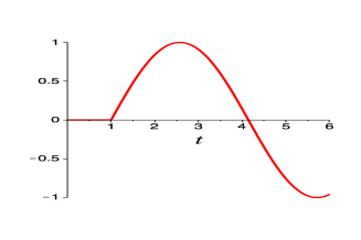
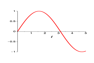
The shifting property of Laplace transform (17) is the reason behind the finite step convergence of the DNWR for a particular value of the parameter θ𝜃\theta. The right hand side of (17) becomes identically zero for tα𝑡𝛼t\leq\alpha, so that for sufficiently small time window length T𝑇T (e.g., Tα𝑇𝛼T\leq\alpha) the error becomes zero and leads to convergence in the next iteration. In Figure 2 we plot 1{f^(s)}superscript1^𝑓𝑠\mathcal{L}^{-1}\left\{\hat{f}(s)\right\} with f(t)=sin(t)𝑓𝑡𝑡f(t)=\sin(t) on the left, and show the effect of time-shifting on the right.
Refer to caption
Refer to caption
Fig. 2: Example of time-shifting for the function f(t)=sin(t)𝑓𝑡𝑡f(t)=\sin(t): 1{f^(s)}superscript1^𝑓𝑠\mathcal{L}^{-1}\left\{\hat{f}(s)\right\} on the left, and 1{esf^(s)}superscript1superscript𝑒𝑠^𝑓𝑠\mathcal{L}^{-1}\left\{e^{-s}\hat{f}(s)\right\} on the right

3 Analysis of NNWR algorithm in 2D

We now formulate and analyze the NNWR algorithm for the two-dimensional wave equation

ttuc2Δu=f(x,y,t),(x,y)Ω=(l,L)×(0,π),t(0,T]formulae-sequenceformulae-sequencesubscript𝑡𝑡𝑢superscript𝑐2Δ𝑢𝑓𝑥𝑦𝑡𝑥𝑦Ω𝑙𝐿0𝜋𝑡0𝑇\partial_{tt}u-c^{2}\Delta u=f(x,y,t),\quad(x,y)\in\Omega=(l,L)\times(0,\pi),\>t\in(0,T]

with initial condition u(x,y,0)=u0(x,y),tu(x,y,0)=v0(x,y)formulae-sequence𝑢𝑥𝑦0subscript𝑢0𝑥𝑦subscript𝑡𝑢𝑥𝑦0subscript𝑣0𝑥𝑦u(x,y,0)=u_{0}(x,y),\partial_{t}u(x,y,0)=v_{0}(x,y) and Dirichlet boundary conditions. To define the Neumann-Neumann algorithm, we decompose ΩΩ\Omega into strips of the form Ωi=(xi1,xi)×(0,π)subscriptΩ𝑖subscript𝑥𝑖1subscript𝑥𝑖0𝜋\Omega_{i}=(x_{i-1},x_{i})\times(0,\pi), l=x0<x1<<xN=L𝑙subscript𝑥0subscript𝑥1subscript𝑥𝑁𝐿l=x_{0}<x_{1}<\cdots<x_{N}=L. We define the subdomain width hi:=xixi1assignsubscript𝑖subscript𝑥𝑖subscript𝑥𝑖1h_{i}:=x_{i}-x_{i-1}, and hmin:=min1iNhiassignsubscriptsubscript1𝑖𝑁subscript𝑖h_{\min}:=\min_{1\leq i\leq N}h_{i}. Also we directly consider the error equations with f(x,y,t)=0,u0(x,y)=0=v0(x,y)formulae-sequence𝑓𝑥𝑦𝑡0subscript𝑢0𝑥𝑦0subscript𝑣0𝑥𝑦f(x,y,t)=0,u_{0}(x,y)=0=v_{0}(x,y) and homogeneous Dirichlet boundary conditions. Given initial guesses {wi0(y,t)}i=1N1superscriptsubscriptsuperscriptsubscript𝑤𝑖0𝑦𝑡𝑖1𝑁1\left\{w_{i}^{0}(y,t)\right\}_{i=1}^{N-1} along the interface {x=xi}𝑥subscript𝑥𝑖\left\{x=x_{i}\right\}, the NNWR algorithm, as a particular case of (2)-(3)-(4), is given by performing iteratively for k=1,2,𝑘12k=1,2,\ldots and for i=1,,N𝑖1𝑁i=1,\ldots,N the Dirichlet and Neumann steps

ttuikc2Δuik=0,in Ωi,ttφikc2Δφik=0,in Ωi,uik(x,y,0)=0,φik(x,y,0)=0,tuik(x,y,0)=0,tφik(x,y,0)=0,uik(xi1,y,t)=wi1k1(y,t),niφik(xi1,y,t)=(ni1ui1k+niuik)(xi1,y,t),uik(xi,y,t)=wik1(y,t),niφik(xi,y,t)=(ni1ui1k+niuik)(xi,y,t),uik(x,0,t)=uik(x,π,t)=0,φik(x,0,t)=φik(x,π,t)=0,subscript𝑡𝑡superscriptsubscript𝑢𝑖𝑘superscript𝑐2Δsuperscriptsubscript𝑢𝑖𝑘0in Ωisubscript𝑡𝑡superscriptsubscript𝜑𝑖𝑘superscript𝑐2Δsuperscriptsubscript𝜑𝑖𝑘0in Ωisuperscriptsubscript𝑢𝑖𝑘𝑥𝑦00superscriptsubscript𝜑𝑖𝑘𝑥𝑦00subscript𝑡superscriptsubscript𝑢𝑖𝑘𝑥𝑦00subscript𝑡superscriptsubscript𝜑𝑖𝑘𝑥𝑦00superscriptsubscript𝑢𝑖𝑘subscript𝑥𝑖1𝑦𝑡superscriptsubscript𝑤𝑖1𝑘1𝑦𝑡subscriptsubscript𝑛𝑖superscriptsubscript𝜑𝑖𝑘subscript𝑥𝑖1𝑦𝑡subscriptsubscript𝑛𝑖1superscriptsubscript𝑢𝑖1𝑘subscriptsubscript𝑛𝑖superscriptsubscript𝑢𝑖𝑘subscript𝑥𝑖1𝑦𝑡superscriptsubscript𝑢𝑖𝑘subscript𝑥𝑖𝑦𝑡superscriptsubscript𝑤𝑖𝑘1𝑦𝑡subscriptsubscript𝑛𝑖superscriptsubscript𝜑𝑖𝑘subscript𝑥𝑖𝑦𝑡subscriptsubscript𝑛𝑖1superscriptsubscript𝑢𝑖1𝑘subscriptsubscript𝑛𝑖superscriptsubscript𝑢𝑖𝑘subscript𝑥𝑖𝑦𝑡superscriptsubscript𝑢𝑖𝑘𝑥0𝑡superscriptsubscript𝑢𝑖𝑘𝑥𝜋𝑡0superscriptsubscript𝜑𝑖𝑘𝑥0𝑡superscriptsubscript𝜑𝑖𝑘𝑥𝜋𝑡0\begin{array}[]{rclrcl}\partial_{tt}u_{i}^{k}-c^{2}\Delta u_{i}^{k}&=&0,\qquad\textrm{in $\Omega_{i}$},&\partial_{tt}\varphi_{i}^{k}-c^{2}\Delta\varphi_{i}^{k}&=&0,\qquad\textrm{in $\Omega_{i}$},\\ u_{i}^{k}(x,y,0)&=&0,&\varphi_{i}^{k}(x,y,0)&=&0,\\ \partial_{t}u_{i}^{k}(x,y,0)&=&0,&\partial_{t}\varphi_{i}^{k}(x,y,0)&=&0,\\ u_{i}^{k}(x_{i-1},y,t)&=&w_{i-1}^{k-1}(y,t),&\partial_{n_{i}}\varphi_{i}^{k}(x_{i-1},y,t)&=&(\partial_{n_{i-1}}u_{i-1}^{k}+\partial_{n_{i}}u_{i}^{k})(x_{i-1},y,t),\\ u_{i}^{k}(x_{i},y,t)&=&w_{i}^{k-1}(y,t),&\partial_{n_{i}}\varphi_{i}^{k}(x_{i},y,t)&=&(\partial_{n_{i-1}}u_{i-1}^{k}+\partial_{n_{i}}u_{i}^{k})(x_{i},y,t),\\ u_{i}^{k}(x,0,t)&=&u_{i}^{k}(x,\pi,t)=0,&\varphi_{i}^{k}(x,0,t)&=&\varphi_{i}^{k}(x,\pi,t)=0,\end{array} (18)

except for the first and last subdomain, where in the Neumann step the Neumann conditions are replaced by homogeneous Dirichlet conditions along the physical boundaries. The update conditions are defined as

wik(y,t)=wik1(y,t)θ(φik(xi,y,t)+φi+1k(xi,y,t)).superscriptsubscript𝑤𝑖𝑘𝑦𝑡superscriptsubscript𝑤𝑖𝑘1𝑦𝑡𝜃superscriptsubscript𝜑𝑖𝑘subscript𝑥𝑖𝑦𝑡superscriptsubscript𝜑𝑖1𝑘subscript𝑥𝑖𝑦𝑡w_{i}^{k}(y,t)=w_{i}^{k-1}(y,t)-\theta\left(\varphi_{i}^{k}(x_{i},y,t)+\varphi_{i+1}^{k}(x_{i},y,t)\right).

We perform a Fourier transform along the y𝑦y direction to reduce the original problem into a collection of one-dimensional problems. Using a Fourier sine series along the y𝑦y-direction, we get

uik(x,y,t)=n1Uik(x,n,t)sin(ny)superscriptsubscript𝑢𝑖𝑘𝑥𝑦𝑡subscript𝑛1superscriptsubscript𝑈𝑖𝑘𝑥𝑛𝑡𝑛𝑦u_{i}^{k}(x,y,t)=\sum_{n\geq 1}U_{i}^{k}(x,n,t)\sin(ny)

where

Uik(x,n,t)=2π0πuik(x,η,t)sin(nη)𝑑η.superscriptsubscript𝑈𝑖𝑘𝑥𝑛𝑡2𝜋superscriptsubscript0𝜋superscriptsubscript𝑢𝑖𝑘𝑥𝜂𝑡𝑛𝜂differential-d𝜂U_{i}^{k}(x,n,t)=\frac{2}{\pi}\int_{0}^{\pi}u_{i}^{k}(x,\eta,t)\sin(n\eta)d\eta.

The NNWR algorithm (18) therefore becomes a sequence of 1D problems for each n𝑛n,

2Uikt2(x,n,t)c22Uikx2(x,n,t)+c2n2Uik(x,n,t)=0,superscript2superscriptsubscript𝑈𝑖𝑘superscript𝑡2𝑥𝑛𝑡superscript𝑐2superscript2superscriptsubscript𝑈𝑖𝑘superscript𝑥2𝑥𝑛𝑡superscript𝑐2superscript𝑛2superscriptsubscript𝑈𝑖𝑘𝑥𝑛𝑡0\frac{\partial^{2}U_{i}^{k}}{\partial t^{2}}(x,n,t)-c^{2}\frac{\partial^{2}U_{i}^{k}}{\partial x^{2}}(x,n,t)+c^{2}n^{2}U_{i}^{k}(x,n,t)=0, (19)

with the boundary conditions for Uik(x,n,t)superscriptsubscript𝑈𝑖𝑘𝑥𝑛𝑡U_{i}^{k}(x,n,t). We now define

χ(α,β,t):=1{exp(βs2+α2)},Re(s)>0,formulae-sequenceassign𝜒𝛼𝛽𝑡superscript1𝛽superscript𝑠2superscript𝛼2Re𝑠0\chi(\alpha,\beta,t):=\mathcal{L}^{-1}\left\{\exp\left(-\beta\sqrt{s^{2}+\alpha^{2}}\right)\right\},\quad\textrm{Re}(s)>0, (20)

with s𝑠s being the Laplace variable. Before presenting the main convergence theorem, we prove the following auxiliary result .

Lemma 3.

We have the identity:

χ(α,β,t)={δ(tβ)αβt2β2J1(αt2β2),tβ,0,0<t<β,𝜒𝛼𝛽𝑡cases𝛿𝑡𝛽𝛼𝛽superscript𝑡2superscript𝛽2subscript𝐽1𝛼superscript𝑡2superscript𝛽2𝑡𝛽00𝑡𝛽\chi(\alpha,\beta,t)=\begin{cases}\delta(t-\beta)-\frac{\alpha\beta}{\sqrt{t^{2}-\beta^{2}}}\,J_{1}\left(\alpha\sqrt{t^{2}-\beta^{2}}\right),&t\geq\beta,\\ 0,&0<t<\beta,\end{cases}

where δ𝛿\delta is the dirac delta function and J1subscript𝐽1J_{1} is the Bessel function of first order given by

J1(z)=1π0πcos(zsinφφ)𝑑φ.subscript𝐽1𝑧1𝜋superscriptsubscript0𝜋𝑧𝜑𝜑differential-d𝜑J_{1}(z)=\frac{1}{\pi}\int_{0}^{\pi}\cos\left(z\sin\varphi-\varphi\right)d\varphi.
Proof.

Using the change of variable r=s2+α2𝑟superscript𝑠2superscript𝛼2r=\sqrt{s^{2}+\alpha^{2}} we write

eβr=eβs(eβseβr).superscript𝑒𝛽𝑟superscript𝑒𝛽𝑠superscript𝑒𝛽𝑠superscript𝑒𝛽𝑟e^{-\beta r}=e^{-\beta s}-(e^{-\beta s}-e^{-\beta r}).

From the table [27, p. 245] we get

1{eβs}=δ(tβ),superscript1superscript𝑒𝛽𝑠𝛿𝑡𝛽\mathcal{L}^{-1}\left\{e^{-\beta s}\right\}=\delta(t-\beta), (21)

Also on page 263 of [27] we find

1{eβseβr}={αβt2β2J1(αt2β2),t>β,0,0<t<β.superscript1superscript𝑒𝛽𝑠superscript𝑒𝛽𝑟cases𝛼𝛽superscript𝑡2superscript𝛽2subscript𝐽1𝛼superscript𝑡2superscript𝛽2𝑡𝛽00𝑡𝛽\mathcal{L}^{-1}\left\{e^{-\beta s}-e^{-\beta r}\right\}=\begin{cases}\frac{\alpha\beta}{\sqrt{t^{2}-\beta^{2}}}\,J_{1}\left(\alpha\sqrt{t^{2}-\beta^{2}}\right),&t>\beta,\\ 0,&0<t<\beta.\end{cases} (22)

Subtracting (22) from (21) we obtain the expected inverse Laplace transform. ∎

Now we are ready to prove the convergence result for NNWR in 2D:

Theorem 4 (Convergence of NNWR in 2D).

Let θ=1/4𝜃14\theta=1/4. For T>0𝑇0T>0 fixed, the NNWR algorithm (18) converges in k+1𝑘1k+1 iterations, if the time window length T𝑇T satisfies T/k<2hmin/c𝑇𝑘2subscript𝑐T/k<2h_{\min}/c, c𝑐c being the wave speed.

Proof.

We take Laplace transforms in t𝑡t of (19) to get

(s2+c2n2)U^ikc2d2U^ikdx2=0,superscript𝑠2superscript𝑐2superscript𝑛2superscriptsubscript^𝑈𝑖𝑘superscript𝑐2superscript𝑑2superscriptsubscript^𝑈𝑖𝑘𝑑superscript𝑥20(s^{2}+c^{2}n^{2})\hat{U}_{i}^{k}-c^{2}\frac{d^{2}\hat{U}_{i}^{k}}{dx^{2}}=0,

and now treat each n𝑛n as in the one-dimensional analysis in the proof of Theorem 1, where the recurrence relations (10), (11) and (12) of the form

w^ik(s)=jAij(k)(s)w^j0(s)superscriptsubscript^𝑤𝑖𝑘𝑠subscript𝑗superscriptsubscript𝐴𝑖𝑗𝑘𝑠superscriptsubscript^𝑤𝑗0𝑠\hat{w}_{i}^{k}(s)=\sum_{j}A_{ij}^{(k)}(s)\hat{w}_{j}^{0}(s) (23)

now become for each n=1,2,𝑛12n=1,2,\ldots

W^ik(n,s)=jAij(k)(s2+c2n2)W^j0(n,s).superscriptsubscript^𝑊𝑖𝑘𝑛𝑠subscript𝑗superscriptsubscript𝐴𝑖𝑗𝑘superscript𝑠2superscript𝑐2superscript𝑛2superscriptsubscript^𝑊𝑗0𝑛𝑠\hat{W}_{i}^{k}(n,s)=\sum_{j}A_{ij}^{(k)}\left(\sqrt{s^{2}+c^{2}n^{2}}\right)\hat{W}_{j}^{0}(n,s). (24)

The equation (23) is of the form (15)-(16), that means Aij(k)(s)superscriptsubscript𝐴𝑖𝑗𝑘𝑠A_{ij}^{(k)}(s) are linear combination of terms of the form eϱssuperscript𝑒italic-ϱ𝑠e^{-\varrho s} for ϱ2khl/citalic-ϱ2𝑘subscript𝑙𝑐\varrho\geq 2kh_{l}/c for some l{1,2,N}𝑙12𝑁l\in\left\{1,2,\ldots N\right\}. Therefore the coefficients Aij(k)(s2+c2n2)superscriptsubscript𝐴𝑖𝑗𝑘superscript𝑠2superscript𝑐2superscript𝑛2A_{ij}^{(k)}\left(\sqrt{s^{2}+c^{2}n^{2}}\right) are sum of exponential functions of the form eϱs2+c2n2superscript𝑒italic-ϱsuperscript𝑠2superscript𝑐2superscript𝑛2e^{-\varrho\sqrt{s^{2}+c^{2}n^{2}}} for ϱ2khl/citalic-ϱ2𝑘subscript𝑙𝑐\varrho\geq 2kh_{l}/c. Hence we use the definition of χ𝜒\chi in (20) to take the inverse Laplace transform of (24), and obtain

Wik(n,t)=jmχ(cn,ϱm,j,t)Wj0(n,t),superscriptsubscript𝑊𝑖𝑘𝑛𝑡subscript𝑗subscript𝑚𝜒𝑐𝑛subscriptitalic-ϱ𝑚𝑗𝑡superscriptsubscript𝑊𝑗0𝑛𝑡W_{i}^{k}(n,t)=\sum_{j}\sum_{m}\chi(cn,\varrho_{m,j},t)*W_{j}^{0}(n,t),

with ϱm,j2khmin/csubscriptitalic-ϱ𝑚𝑗2𝑘subscript𝑐\varrho_{m,j}\geq 2kh_{\min}/c. So it is straightforward that for t<2khmin/c𝑡2𝑘subscript𝑐t<2kh_{\min}/c, Wik(n,t)=0superscriptsubscript𝑊𝑖𝑘𝑛𝑡0W_{i}^{k}(n,t)=0 for each n𝑛n, since the function χ𝜒\chi is zero there by Lemma 3. Therefore the interface functions wik(y,t)superscriptsubscript𝑤𝑖𝑘𝑦𝑡w_{i}^{k}(y,t), given by wik(y,t)=n1Wik(n,t)sin(ny)superscriptsubscript𝑤𝑖𝑘𝑦𝑡subscript𝑛1superscriptsubscript𝑊𝑖𝑘𝑛𝑡𝑛𝑦w_{i}^{k}(y,t)={\displaystyle{\displaystyle\sum_{n\geq 1}}}W_{i}^{k}(n,t)\sin(ny) are also zero for all i{1,,N1}𝑖1𝑁1i\in\left\{1,\ldots,N-1\right\}. Hence one more iteration produces the desired solution on the entire domain. ∎

4 Numerical Experiments

We perform numerical experiments to see the convergence behavior of the NNWR algorithm with multiple subdomains for the model problem

ttusubscript𝑡𝑡𝑢\displaystyle\partial_{tt}u =c2(x)xxu,absentsuperscript𝑐2𝑥subscript𝑥𝑥𝑢\displaystyle=c^{2}(x)\partial_{xx}u, x(0,5),t>0,formulae-sequence𝑥05𝑡0\displaystyle x\in(0,5),t>0,
u(x,0)𝑢𝑥0\displaystyle u(x,0) =0,ut(x,0)=0,formulae-sequenceabsent0subscript𝑢𝑡𝑥00\displaystyle=0,\>u_{t}(x,0)=0, 0<x<5,0𝑥5\displaystyle 0<x<5, (25)
u(0,t)𝑢0𝑡\displaystyle u(0,t) =t2,u(5,t)=t2et,formulae-sequenceabsentsuperscript𝑡2𝑢5𝑡superscript𝑡2superscript𝑒𝑡\displaystyle=t^{2},\>u(5,t)=t^{2}e^{-t}, t>0,𝑡0\displaystyle t>0,

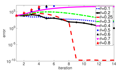
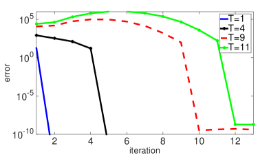
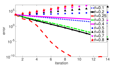
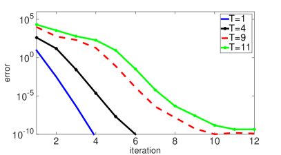
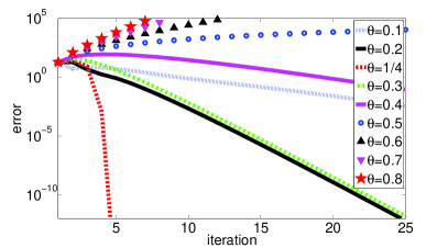
which is discretized using centered finite differences in both space and time on a grid with Δx=Δt=2×10²Δ𝑥Δ𝑡2superscript102\Delta x=\Delta t=2{\times}10^{-2}. We consider a decomposition of (0,5)05(0,5) into five unequal subdomains, whose widths hisubscript𝑖h_{i} are 0.6,0.6,0.5,2.3,10.60.60.52.310.6,0.6,0.5,2.3,1 respectively, and take the initial guesses wj0(t)=t2,t(0,T]formulae-sequencesuperscriptsubscript𝑤𝑗0𝑡superscript𝑡2𝑡0𝑇w_{j}^{0}(t)=t^{2},t\in(0,T] for 1j41𝑗41\leq j\leq 4. Note that in some of the experiments below, the coefficient c(x)𝑐𝑥c(x) will be spatially varying. This will allow us to study how spatially varying coefficients affect the performance of the NNWR, which have only been analyzed in the constant coefficient case. For the first experiment, we take the constant speed, c=1𝑐1c=1. On the left panel of Figure 3, we show the convergence for different values of the parameter θ𝜃\theta for T=8𝑇8T=8, and on the right the results for the best parameter θ=1/4𝜃14\theta=1/4 for different time window length T𝑇T. We observe two-step convergence for θ=1/4𝜃14\theta=1/4 for a sufficiently small time window T𝑇T. Now we take the propagation speed, c(x)=(x+1)/6𝑐𝑥𝑥16c(x)=(x+1)/6 for the second experiment. On the left panel of Figure 4, we show the convergence for different values of the parameter θ𝜃\theta for T=8𝑇8T=8, and on the right the results for the best parameter θ=1/4𝜃14\theta=1/4 for different time window length T𝑇T.

Refer to caption
Refer to caption
Fig. 3: Convergence of NNWR with various values of θ𝜃\theta for T=8𝑇8T=8 on the left, and for various lengths T𝑇T of the time window and θ=1/4𝜃14\theta=1/4 on the right
Refer to caption
Refer to caption
Fig. 4: Convergence of NNWR for variable coefficients c(x)=(x+1)/6𝑐𝑥𝑥16c(x)=(x+1)/6 with various values of θ𝜃\theta for T=8𝑇8T=8 on the left, and for various lengths T𝑇T of the time window and θ=1/4𝜃14\theta=1/4 on the right

Next we show an experiment for the NNWR algorithm in two dimension for the following model problem

ttu(xxu+yyu)=0,u(x,y,0)=xy(x1)(yπ)(5x2)(4x3),ut(x,y,0)=0,formulae-sequencesubscript𝑡𝑡𝑢subscript𝑥𝑥𝑢subscript𝑦𝑦𝑢0formulae-sequence𝑢𝑥𝑦0𝑥𝑦𝑥1𝑦𝜋5𝑥24𝑥3subscript𝑢𝑡𝑥𝑦00\partial_{tt}u-\left(\partial_{xx}u+\partial_{yy}u\right)=0,u(x,y,0)=xy(x-1)(y-\pi)(5x-2)(4x-3),u_{t}(x,y,0)=0,

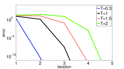
with homogeneous Dirichlet boundary conditions. We discretize the wave equation using the centered finite difference in both space and time (Leapfrog scheme) on a grid with Δx=5×10²,Δy=16×102,Δt=4×10²formulae-sequenceΔ𝑥5superscript102formulae-sequenceΔ𝑦16superscript102Δ𝑡4superscript102\Delta x=5{\times}10^{-2},\Delta y=16{\times}10^{-2},\Delta t=4{\times}10^{-2}. We decompose our domain Ω:=(0,1)×(0,π)assignΩ010𝜋\Omega:=(0,1)\times(0,\pi) into three non-overlapping subdomains Ω1=(0,2/5)×(0,π)subscriptΩ10250𝜋\Omega_{1}=(0,2/5)\times(0,\pi), Ω2=(2/5,3/4)×(0,π)subscriptΩ225340𝜋\Omega_{2}=(2/5,3/4)\times(0,\pi), Ω3=(3/4,1)×(0,π)subscriptΩ33410𝜋\Omega_{3}=(3/4,1)\times(0,\pi). As initial guesses, we take wi0(y,t)=tsin(y)superscriptsubscript𝑤𝑖0𝑦𝑡𝑡𝑦w_{i}^{0}(y,t)=t\sin(y). In Figure 5 we plot the convergence curves for different values of the parameter θ𝜃\theta for T=2𝑇2T=2 on the left panel, and on the right the results for the best parameter θ=1/4𝜃14\theta=1/4 for different time window length T𝑇T.

Refer to caption
Refer to caption
Fig. 5: Convergence of NNWR in 2D: curves for different values of θ𝜃\theta for T=2𝑇2T=2 on the left, and for various time lengths T𝑇T and θ=1/4𝜃14\theta=1/4 on the right

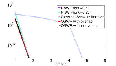
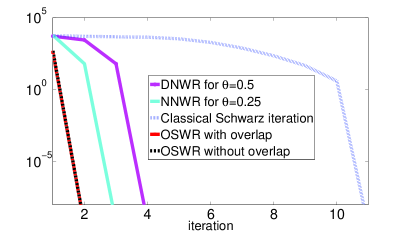
We compare in Figure 6 the performance of the NNWR and DNWR (see [12]) algorithms with the SWR algorithms with and without overlap. Here we consider the problem

ttuxxusubscript𝑡𝑡𝑢subscript𝑥𝑥𝑢\displaystyle\partial_{tt}u-\partial_{xx}u =0,absent0\displaystyle=0, x(3,2),t>0,formulae-sequence𝑥32𝑡0\displaystyle x\in(-3,2),t>0,
u(x,0)𝑢𝑥0\displaystyle u(x,0) =0,ut(x,0)=xex,formulae-sequenceabsent0subscript𝑢𝑡𝑥0𝑥superscript𝑒𝑥\displaystyle=0,\>u_{t}(x,0)=xe^{-x}, 3<x<2,3𝑥2\displaystyle-3<x<2,
u(3,t)𝑢3𝑡\displaystyle u(-3,t) =3e3t,u(2,t)=2te2,formulae-sequenceabsent3superscript𝑒3𝑡𝑢2𝑡2𝑡superscript𝑒2\displaystyle=-3e^{3}t,\>u(2,t)=2te^{-2}, t>0,𝑡0\displaystyle t>0,

and for the overlapping Schwarz variant we use an overlap of length 24Δx24Δ𝑥24\Delta x, where Δx=1/50Δ𝑥150\Delta x=1/50. For the DNWR, NNWR and non-overlapping SWR we consider a domain decomposition into two subdomains Ω1=(3,0)subscriptΩ130\Omega_{1}=(-3,0) and Ω2=(0,2)subscriptΩ202\Omega_{2}=(0,2). We observe that the DNWR and NNWR algorithms converge as fast as the Schwarz WR algorithms for smaller time windows T𝑇T.

Refer to caption
Refer to caption
Fig. 6: Comparison of DNWR, NNWR, and SWR for 1D wave equation for T=4𝑇4T=4 on the left, and T=10𝑇10T=10 on the right
Table 1: Comparison of steps needed for convergence for 1D wave equation.
Methods 2 subdomains, 1D Many subdomains, 1D Many subdomains, 2D
DNWR T2khmin/c𝑇2𝑘subscript𝑐T\leq 2kh_{\min}/c Tkhmin/c𝑇𝑘subscript𝑐T\leq kh_{\min}/c T<khmin/c𝑇𝑘subscript𝑐T<kh_{\min}/c
NNWR T4khmin/c𝑇4𝑘subscript𝑐T\leq 4kh_{\min}/c T2khmin/c𝑇2𝑘subscript𝑐T\leq 2kh_{\min}/c T<2khmin/c𝑇2𝑘subscript𝑐T<2kh_{\min}/c

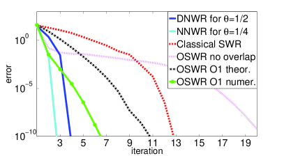
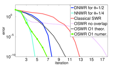
Due to the local nature of the Dirichlet-to-Neumann operator in 1D [8], SWR converges in a finite number of iterations just like DNWR and NNWR. In higher dimensions, however, non-overlapping SWR will no longer converge in a finite number of steps, but DNWR and NNWR will; see Figure 7. Table 1 gives a summary of the theoretical results from Section 2 and 3 and [12], to indicate the maximum number of iterations needed for the 1D and 2D wave equation to converge to the exact solution. For the comparison result in 2D, we consider the model problem

ttu(xxu+yyu)=0,u(x,y,0)=0=ut(x,y,0),formulae-sequencesubscript𝑡𝑡𝑢subscript𝑥𝑥𝑢subscript𝑦𝑦𝑢0𝑢𝑥𝑦00subscript𝑢𝑡𝑥𝑦0\partial_{tt}u-\left(\partial_{xx}u+\partial_{yy}u\right)=0,u(x,y,0)=0=u_{t}(x,y,0),

with Dirichlet boundary conditions u(0,y,t)=t2sin(y),u(1,y,t)=y(yπ)t3formulae-sequence𝑢0𝑦𝑡superscript𝑡2𝑦𝑢1𝑦𝑡𝑦𝑦𝜋superscript𝑡3u(0,y,t)=t^{2}\sin(y),u(1,y,t)=y(y-\pi)t^{3} and u(x,0,t)=0=u(x,π,t)𝑢𝑥0𝑡0𝑢𝑥𝜋𝑡u(x,0,t)=0=u(x,\pi,t). We decompose our domain Ω:=(0,1)×(0,π)assignΩ010𝜋\Omega:=(0,1)\times(0,\pi) for the two subdomains experiment into Ω1=(0,3/5)×(0,π)subscriptΩ10350𝜋\Omega_{1}=(0,3/5)\times(0,\pi) and Ω2=(3/5,1)×(0,π)subscriptΩ23510𝜋\Omega_{2}=(3/5,1)\times(0,\pi), and for the three subdomains experiment into Ω1=(0,2/5)×(0,π)subscriptΩ10250𝜋\Omega_{1}=(0,2/5)\times(0,\pi), Ω2=(2/5,3/4)×(0,π)subscriptΩ225340𝜋\Omega_{2}=(2/5,3/4)\times(0,\pi), Ω3=(3/4,1)×(0,π)subscriptΩ33410𝜋\Omega_{3}=(3/4,1)\times(0,\pi). We take a random initial guess to start the iteration, and for the overlapping SWR we use an overlap of length 2Δx2Δ𝑥2\Delta x in all the experiments. We implement first order methods with one parameter in optimized SWR iterations; for more details see [5]. On the left panel of Figure 7 we plot the comparison curves for two subdomains, and the same for three subdomains on the right.
Refer to caption
Refer to caption
Fig. 7: Comparison of DNWR, NNWR, and SWR for T=2𝑇2T=2 in 2D for two subdomains on the left, and three subdomains on the right

Now we show a numerical experiment for the NNWR algorithm with different time grids for different subdomains and discontinuous wave speed across interfaces. We consider the model problem

ttuc2xxu=0,u(x,0)=0=ut(x,0),formulae-sequencesubscript𝑡𝑡𝑢superscript𝑐2subscript𝑥𝑥𝑢0𝑢𝑥00subscript𝑢𝑡𝑥0\partial_{tt}u-c^{2}\partial_{xx}u=0,u(x,0)=0=u_{t}(x,0),

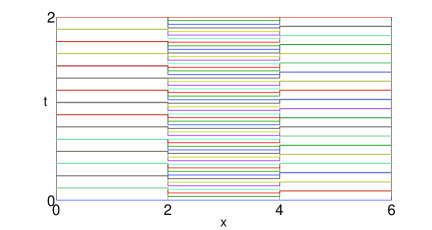
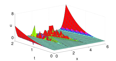
with Dirichlet boundary conditions u(0,t)=t2,u(6,t)=t3formulae-sequence𝑢0𝑡superscript𝑡2𝑢6𝑡superscript𝑡3u(0,t)=t^{2},u(6,t)=t^{3}. Suppose the spatial domain Ω:=(0,6)assignΩ06\Omega:=(0,6) is decomposed into three equal subdomains Ωi,i=1,2,3formulae-sequencesubscriptΩ𝑖𝑖123\Omega_{i},i=1,2,3, and the random initial guesses are used to start the NNWR iteration. For the spatial discretization, we take a uniform mesh with size Δx=1×101Δ𝑥1superscript101\Delta x=1{\times}10^{-1}, and for the time discretization, we use non-uniform time grids Δti,i=1,2,3formulae-sequenceΔsubscript𝑡𝑖𝑖123\Delta t_{i},i=1,2,3, as given in Table 2. For the non-uniform mesh grid, boundary data is transmitted from one subdomain to a neighboring subdomain by introducing a suitable time projection. For two dimensional problems, the interface is one dimensional. Using ideas of merge sort one can compute the projection with linear cost, see [9] and the references therein. Even for higher dimensional interfaces, such an algorithm with linear complexity is still possible, see [10]. In Figure 8 we show the non-uniform time steps for different subdomains. Figure 9 gives the convergence behavior of the NNWR algorithm for T=2𝑇2T=2 with the same non-uniform time grids as in Table 2.

Table 2: Propagation speed and time steps for different subdomains.
Ω1subscriptΩ1\Omega_{1} Ω2subscriptΩ2\Omega_{2} Ω3subscriptΩ3\Omega_{3}
wave speed c𝑐c 1/4141/4 222 1/2121/2
time grids ΔtiΔsubscript𝑡𝑖\Delta t_{i} 13×10213superscript10213\times 10^{-2} 39×10339superscript10339\times 10^{-3} 1×10¹¹superscript1011\times 10^{-1}
Refer to caption
Fig. 8: Subdomains with non-uniform time steps
Refer to caption
Refer to caption
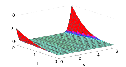
Fig. 9: Solution using NNWR method for the wave equation with non-uniform time steps for θ=1/4𝜃14\theta=1/4 for T=2𝑇2T=2: Solution after 1st iteration on the left, and solution after 2nd iteration on the right

Finally we raise the issue of scalability of the NNWR algorithm by giving some numerical examples for the wave equation. From Theorem 1, one can say that as long as h/T𝑇h/T is constant, we expect identical convergence behavior of the NNWR algorithm. We plot in Figure 10 the convergence curves by doubling the number of subdomains and making the time window length half. One can therefore conclude that the NNWR algorithm is weakly scalable for the wave equation.
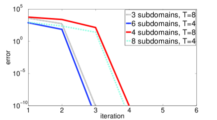
Refer to caption
Fig. 10: Graphs for comparing scalability of NNWR method for the wave equation

5 Conclusions

We defined the NNWR algorithm for multiple subdomains and for general hyperbolic problems, and analyzed their convergence properties for the second order wave equation in 1D. We showed using numerical experiments that for a particular choice of the relaxation parameter, more specifically for θ=1/4𝜃14\theta=1/4, convergence can be achieved in a finite number of steps. In fact, this algorithm can be used as a two-step method, choosing the time window lengh T𝑇T small enough. We have also extended the NNWR algorithm for the second order wave equation in 2D, and analyzed its convergence properties. We have also shown using numerical experiments that among the DNWR (see [11]) and NNWR methods, NNWR converges faster. But in comparison to DNWR, the NNWR has to solve twice the number of subproblems (once for Dirichlet subproblems, and once for Neumann subproblems) on each subdomain at each iteration. Therefore the computational cost is almost double for the NNWR than for the DNWR algorithm at each step. However, we get better convergence behavior with the NNWR in terms of iteration numbers. Finally we presented a comparison of performences between the DNWR, NNWR and Schwarz WR methods, and showed that the DNWR and NNWR converge faster than optimized SWR at least for higher dimensions.

Acknowledgement

I would like to express my gratitude to Prof. Martin J. Gander and Prof. Felix Kwok for their constant support and stimulating suggestions.

References

  • [1] J. F. Bourgat, R. Glowinski, P. L. Tallec, and M. Vidrascu, Variational Formulation and Algorithm for Trace Operator in Domain Decomposition Calculations, in Domain Decomposition Methods, T. F. Chan, R. Glowinski, J. Périaux, and O. B. Widlund, eds., SIAM, 1989, pp. 3–16.
  • [2] X.-C. Cai, Additive Schwarz algorithms for parabolic convection-diffusion equations, Numer. Math., 60 (1991), pp. 41–61.
  • [3]  , Multiplicative Schwarz Methods for Parabolic Problems, SIAM J. Sci. Comput., 15 (1994), pp. 587–603.
  • [4] M. J. Gander, Optimized Schwarz methods, SIAM J. Numer. Anal., 44 (2006), pp. 699–732.
  • [5] M. J. Gander and L. Halpern, Absorbing Boundary Conditions for the Wave Equation and Parallel Computing, Math. of Comput., 74 (2004), pp. 153–176.
  • [6]  , Optimized Schwarz Waveform Relaxation for Advection Reaction Diffusion Problems, SIAM J. Num. Anal., 45 (2007), pp. 666–697.
  • [7] M. J. Gander, L. Halpern, and F. Nataf, Optimal convergence for overlapping and non-overlapping Schwarz waveform relaxation, in 11th International Conference on Domain Decomposition in Science and Engineering, C.-H. Lai, P. E. Bjørstad, M. Cross, and O. B. Widlund, eds., 1999, pp. 253–260.
  • [8]  , Optimal Schwarz Waveform Relaxation for the One Dimensional Wave Equation, SIAM J. Num. Anal., 41 (2003), pp. 1643–1681.
  • [9] M. J. Gander and C. Japhet, An Algorithm for Non-Matching Grid Projections with Linear Complexity, in Domain Decomposition in Science and Engineering XVIII, M. Bercovier, M. J. Gander, D. Keyes, and O. Widlund, eds., 2008.
  • [10]  , Algorithm 932: PANG: Software for Non-Matching Grid Projections in 2d and 3d with Linear Complexity, ACM Transactions on Mathematical Software (TOMS), 40 (2013), pp. 6:1–6:25.
  • [11] M. J. Gander, F. Kwok, and B. C. Mandal, Dirichlet-Neumann Waveform Relaxation Method for the 1D and 2D Heat and Wave Equations in Multiple subdomains, in Preparation.
  • [12]  , Dirichlet-Neumann and Neumann-Neumann Waveform Relaxation for the Wave Equation, in Domain Decomposition in Science and Engineering XXII, Springer-Verlag, 2015.
  • [13]  , Dirichlet-Neumann and Neumann-Neumann Waveform Relaxation Algorithms for Parabolic Problems, submitted, (arXiv:1311.2709).
  • [14] M. J. Gander and A. M. Stuart, Space-time continuous analysis of waveform relaxation for the heat equation, SIAM J. for Sci. Comput., 19 (1998), pp. 2014–2031.
  • [15] E. Giladi and H. Keller, Space time domain decomposition for parabolic problems, Tech. Report 97-4, Center for research on parallel computation CRPC, Caltech, 1997.
  • [16] J. Janssen and S.: Vandewalle, Multigrid Waveform Relaxation on Spatial Finite Element Meshes: The Continuous-time Case, SIAM J. Numer. Anal., 33 (1996), pp. 456–474.
  • [17] R. Jeltsch and B. Pohl, Waveform relaxation with overlapping splittings, SIAM J. Sci. Comput., (1995).
  • [18] F. Kwok, Neumann-Neumann Waveform Relaxation for the Time-Dependent Heat Equation, in Domain Decomposition in Science and Engineering XXI, J. Erhel, M. J. Gander, L. Halpern, G. Pichot, T. Sassi, and O. B. Widlund, eds., vol. 98, Springer-Verlag, 2014, pp. 189–198.
  • [19] E. Lelarasmee, A. Ruehli, and A. Sangiovanni-Vincentelli, The waveform relaxation method for time-domain analysis of large scale integrated circuits, IEEE Trans. Compt.-Aided Design Integr. Circuits Syst., 1 (1982), pp. 131–145.
  • [20] E. Lindelöf, Sur l’application des méthodes d’approximations successives à l’étude des intégrales réelles des équations différentielles ordinaires, Journal de Mathématiques Pures et Appliquées, (1894).
  • [21] C. Lubich and A. Ostermann, Multigrid dynamic iteration for parabolic equations, BIT, 27 (1987), pp. 216–234.
  • [22] B. C. Mandal, Convergence Analysis of Substructuring Waveform Relaxation Methods for Space-time Problems and Their Application to Optimal Control Problems, 2014. Thesis (Ph.D.)–University of Geneva.
  • [23]  , A Time-Dependent Dirichlet-Neumann Method for the Heat Equation, in Domain Decomposition in Science and Engineering XXI, J. Erhel, M. J. Gander, L. Halpern, G. Pichot, T. Sassi, and O. B. Widlund, eds., vol. 98, Springer-Verlag, 2014, pp. 467–475.
  • [24] V. Martin, An optimized Schwarz waveform relaxation method for unsteady convection diffusion equation, Appl. Numer. Math., 52 (2005), pp. 401–428.
  • [25] E. Picard, Sur l’application des méthodes d’approximations successives à l’étude de certaines équations différentielles ordinaires, Journal de Mathématiques Pures et Appliquées, (1893).
  • [26] Y. D. Roeck and P. L. Tallec, Analysis and Test of a local domain decomposition preconditioner, in Domain Decomposition Methods for PDEs, I, R. Glowinski et al., ed., Philadelphia, 1991, SIAM, pp. 112–128.
  • [27] J. L. Schiff, The Laplace Transform, Springer, 1991.
  • [28] P. L. Tallec, Y. D. Roeck, and M. Vidrascu, Domain decomposition methods for large linearly elliptic three-dimensional problems, J. of Comput. and App. Math., (1991).
  • [29] A. Toselli and O. B. Widlund, Domain Decomposition Methods, Algorithms and Theory, Springer, 2005.