Satellite content and quenching of star formation in galaxy groups at $z\sim 1.8$

We study the properties of satellites in the environment of massive star-forming galaxies at $z\sim 1.8$ in the COSMOS field, using a sample of 215 galaxies on the main sequence of star formation with an average mass of $\sim 10^{11}$ M_⊙. At $z>1.5$, these galaxies typically trace halos of mass $\gtrsim 10^{13}$ M_⊙. We use optical-near-infrared photometry to estimate stellar masses and star formation rates (SFR) of centrals and satellites down to $\sim 6\times 10^{9}$ M_⊙. We stack data around 215 central galaxies to statistically detect their satellite halos, finding an average of $\sim 3$ galaxies in excess of the background density. We fit the radial profiles of satellites with simple $\beta$-models, and compare their integrated properties to model predictions. We find that the total stellar mass of satellites amounts to $\sim 68$% of the central galaxy, while SED modeling and far-infrared photometry consistently show their total SFR to be $25-35$% of the central’s rate. We also see significant variation in the specific SFR of satellites within the halo with, in particular, a sharp decrease at $<100$ kpc. After considering different potential explanations, we conclude that this is likely an environmental signature of the hot inner halo. This effect can be explained in the first order by a simple free-fall scenario, suggesting that these low-mass environments can shut down star formation in satellites on relatively short timescales of $\sim 0.3$ Gyr.

1 Introduction

Although the gradual infall of small dark matter halos onto larger ones has become a relatively straightforward aspect of the standard hierarchical formation paradigm, what happens to the baryons they contain is less well understood. In particular, the mechanisms that drive the evolution of their constituent galaxies become more complex as they are accreted by larger structures. Of special relevance are the processes that regulate and ultimately suppress star formation in galaxies in the early Universe. Their relationship to, and influence on, the galaxies’ immediate environment is not known with certainty; also debated is the relative importance of internal mechanisms versus externally driven ones (although the former are expected to be dominant in massive systems and the latter to act preferentially on lower-mass satellite galaxies; e.g., Baldry et al., 2006; Peng et al., 2010; Gabor et al., 2011). The $z=1.5-2.5$ epoch is particularly interesting as a transition period when global star formation in the universe peaks, but also where the first ostensibly collapsed and virialized galaxy structures appear, in which a spatial segregation of different galaxy types (e.g., passive and active) is observed. In particular, the cores of massive clusters appear to become dominated by quiescent galaxies around this time (e.g., Spitler et al., 2012; Strazzullo et al., 2013; Gobat et al., 2013). From a theoretical point of view, the increasing temperature of the gaseous medium in group- and cluster-scale halos starts to efficiently prevent accretion around this epoch (e.g., Dekel & Birnboim, 2006; Dekel et al., 2009), thus affecting the build-up and evolution of the galaxies they host. One can therefore expect the processes regulating mass accretion onto galaxies, crucial to our understanding of galaxy build-up, to be relatively accessible to observation at this epoch.

For practical and historical reasons, the mass regime most often explored at high redshift has been that of large galaxy clusters, which are the richest and most readily selectable halos. They are also the most biased regions in which to study environmental effects on galaxy evolution. However, at high redshift the advantages offered to galaxy evolution studies by their galaxy density and mass contrast are somewhat counterbalanced by their relative rarity. A lot of effort has thus been devoted to the search for high-redshift structures, through a variety of methods. Although remarkable progress has been made recently, only a handful of $z>1.5$ structures have been accurately characterized so far (e.g., Andreon et al., 2009; Papovich et al., 2010; Gobat et al., 2011; Stanford et al., 2012), as this endeavor is still fundamentally hampered by the relatively limited area for which deep datasets are available (although this may change thanks to ongoing and future deep wide-field infrared surveys). On the other hand, the lower “group” mass range, at this redshift that of the progenitors of $z=0$ clusters, has been less systematically explored; it requires either much deeper data (e.g., Erfaniar et al., 2013; Tanaka et al., 2013) or tracers, such as specific galaxy types (e.g., quasars or giant radio-galaxies), that correlate with structures but are not directly proportional to mass (unlike, e.g., galaxy density or diffuse X-ray emission). This latter type of tracer has been historically used for higher redshift systems, such as proto-clusters (e.g., Hatch et al., 2011; Wylezalek et al., 2013). At lower halo masses, even isolated massive galaxies are expected to be at the center of galaxy assemblages, as a simple consequence of the hierarchical nature of matter distribution in the universe.

In Béthermin et al. (2014), we indeed found that massive ($\sim 10^{11}$ M_⊙), star-forming galaxies on the main sequence of star formation (e.g., Brinchmann et al., 2004; Daddi et al., 2007; Rodighiero et al., 2010) in the range $z=1.5-2.5$ had clustering properties consistent with halos of mass ($>10^{13}$ M_⊙). Subsequent stacking of deep X-ray datasets available in COSMOS yielded constraints on the total mass consistent with the clustering analysis ($\sim 2\times 10^{13}$ M_⊙), thus providing independent confirmation. This suggests that massive main-sequence galaxies constitute a conspicuous tracer of group-scale environments at $z\sim 2$ (more so than, e.g., isolated quiescent galaxies), thus allowing for the easy study of these systems.

Small halos comprising a central galaxy and its satellite system are particularly useful for probing the environmental dependency of galaxy properties over large mass and redshift ranges. In particular, they provide a powerful tool to constrain quenching mechanisms and timescales, through their tell-tale signature on mass profiles and functions (e.g., Wang et al., 2010, 2014; Phillips et al., 2014; Hartley et al., 2015) or simple derived quantities such as the fraction of quiescent satellites (e.g., George et al., 2011). Being vastly more abundant and structurally simpler than massive galaxy clusters, these systems allow for a straightforward test for galaxy assembly and evolution models (e.g., Guo et al., 2011), without requiring deep knowledge of their components (age, position in phase-space, etc.). Here we have taken an intermediate approach, focusing on the properties of star-forming satellites, and in particular on the variation of their star formation rates (SFR). We have only considered systems with massive star-forming centrals: while quiescent galaxy pairs also trace similar sized halos (Béthermin et al., 2014), their center of mass is less clear, which would make an investigation of the radial dependency of satellite properties less straightforward. This paper is organized as follows: in Section 2, we describe the dataset and our sample selection. In Section 3, we present the integrated properties of satellites and the method used to derive them. In Section 4, we discuss their variation with environment and present our conclusions in Section 5. Throughout this paper we assume a $\Lambda$CDM cosmology with $H_{0}=70$ km s^-1 Mpc^-1, $\Omega_{m}=0.27$, and $\Lambda=0.73$, and a Chabrier (2003) initial mass function (IMF; relations used here that assume a different IMF have been converted to this one). Magnitudes are given in the AB photometric system throughout.

2 Data and sample selection

In this work, we have used aperture-corrected photometry from the $K_{s}$-selected catalog of the COSMOS/UltraVISTA survey (McCracken et al., 2012) from Muzzin et al. (2013). We have adopted photometric redshifts ($z_{phot}$) from Ilbert et al. (2013, and references therein) rather than the $z_{phot}$ estimates from Muzzin et al. (2013), as the former had access to a larger and deeper training set of spectroscopic redshifts ($z_{spec}$) (especially zCOSMOS Deep; Lilly et al., 2007), ensuring greater reliability of $z_{phot}$ at $z>1$. For objects for which these were not available, we have used the $z_{phot}$ estimates from Muzzin et al. (2013). Where possible, we have also used $z_{spec}$ from the zCOSMOS Bright sample (Lilly et al., 2009). Stellar masses, SFR, and rest-frame colors were then recomputed based on this merged catalog, as described in Section 2.1. Finally, we have also used mid- and far-infrared (FIR) maps from Spitzer/MIPS (Le Floc’h et al., 2009), Herschel/PACS (from the PEP survey; Lutz et al., 2011), and Herschel/SPIRE (from the HerMES survey; Oliver et al., 2012) in the analysis, although only the PACS data were used for the construction of the sample (see below).

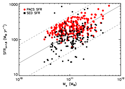
Figure 1: SFR of centrals as a function of their stellar mass, for SFR estimates from, respectively, Herschel/PACS fluxes (red circles) and SED modeling (black squares). Our adopted parametrization of the main sequence at $z=1.8$ is shown as a gray line, with the 0.5 dex limit shown by dashed lines. The SFRs shown here have been corrected according to the difference in normalization between the main sequence at $z=1.8$ and the redshift of the objects.

For consistency with Béthermin et al. (2014), we have built a sample of massive, star-forming galaxies by considering all BzK-selected (Daddi et al., 2004), Herschel/PACS-detected objects with SFRs within 0.5 dex of the main sequence (as parametrized in Béthermin et al., 2012), using the recomputed stellar mass derived from the UV-near-infrared (NIR) photometry and SFR derived from fits to the $100$ and $160\mu$ fluxes with Magdis et al. (2012) templates. Selecting only PACS-detected sources mostly yields massive galaxies, while the 0.5 dex removes lower and upper outliers (e.g., quenching galaxies and starbursts, respectively). The position of galaxies in our sample, relative to the main sequence at $z=1.8$, is shown in Fig. 1. In addition, we have also rejected galaxies that are less than 1′ ($\sim 500$ kpc) away from known overdensities with redshifts consistent within the 68% confidence level (Chiang et al., 2014; Strazzullo et al., 2015), or probable companions (also with redshifts consistent at 68% confidence) of mass $m_{frac}\geq 2$ times higher within $r_{vir}=35$″ ($\sim 300$ kpc). This constraint corresponds roughly to the typical expected virial radius ($r_{vir}$) of a $\sim 2\times 10^{13}$ M_⊙ halo in the sample’s redshift range ($1.5\lesssim z\lesssim 2.5$), while the constraint on the mass ratio between the central and companion galaxy reflects the typical stellar mass uncertainty when all variables and degeneracies are taken into account (e.g., Berta et al., 2004; Conroy, 2013). The first criterion is conservative and meant to minimize the risk of including halos significantly more massive than $\sim 2\times 10^{13}$ M_⊙. Such systems would also be richer and might somewhat bias the results of our analysis. These values, although physically motivated, were also chosen as a compromise to obtain a relatively clean but still statistically significant sample. We note that altering them slightly (e.g., $m_{frac}=1$ and $r=5$″ so as to reject probable interacting pairs) does not change the sample much, nor the outcome of the analysis presented below. This criterion yields 215 galaxies, which we henceforth assume are central to their halo (hereafter, centrals), with a mean mass of $\langle$M${}_{\star}\rangle=1.3\times 10^{11}$ M_⊙ and a mean redshift of $\langle z\rangle=1.8$. The scatter of the centrals’ stellar mass distribution is $\sim 0.25$ dex, consistent with that expected from a single halo population at this redshift (Behroozi et al., 2013). The distribution of masses and redshifts in the sample is shown in Fig. 2.

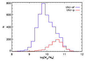
Figure 2: Distribution of stellar masses (left) and redshifts (middle) of centrals in our sample, and of stellar masses of satellites (right) color-selected as star-forming (blue histogram) and quiescent (red histogram).

2.1 Stellar population modeling

We have estimated stellar masses, SFR, and dust extinction for both centrals and satellites (see Section 3) by fitting the available UV-NIR SEDs with two different types of Bruzual & Charlot (2003) models: stellar masses were computed assuming a generalistic delayed exponential star formation history (SFH) of the form SFR(t) = SFR${}_{0}\times(t/\tau^{2})\times\textrm{exp}(-t/\tau)$ which includes both rising and declining cases. The age $t$ and timescale $\tau$ were allowed to vary between 0.1 Gyr ($t$) or 1 Myr ($\tau$) and the age of the Universe at the redshift of the galaxy. Star formation and extinction values, on the other hand, were estimated by fitting the rest-frame UV photometry assuming a constant SFR with an age limit of $t>100$ Myr (the timescale explicitly assumed for UV-derived SFRs; e.g., Kennicutt, 1998). This was done because, while the rest-frame optical-NIR part of the SED reflects the entire SFH of the galaxy, the rest-frame UV part is sensitive to “instant” SFR. This also makes comparison with the literature easier, since direct UV-to-SFR conversions (Kennicutt, 1998) generally assume continuous star formation over $\sim 100$ Myr (see also Section 4). We have included extinction by dust, considering values of $E(B$-$V)\leq 2$ and assuming a Calzetti et al. (2000) functional form with an additional UV bump (Noll et al., 2009; Buat et al., 2012). This limit should be safely above the normal values for even the most massive centrals in our sample (e.g., Garn & Best, 2010; Zahid et al., 2014; Pannella et al., 2014). Solar metallicity was assumed for all models: due to the age-metallicity degeneracy, this parameter would only matter in the case of very old populations, which are not liable to be relevant for the galaxies we consider in our analysis. We have ignored the far- and near-UV GALEX bands, as the resolution of GALEX is significantly poorer than that of the other instruments contributing to the catalog ($>4$″ compared to sub-arcsecond seeing), which precludes efficient deblending on scales typical of the size of halo cores ($\sim 5$″, and thus relevant to the analysis in Section 4). For the same reason, we did not include the 5.8 and 8 $\mu$m Spitzer/IRAC bands in the modeling and treated the FIR data separately, as detailed in Section 3.1. The SED modeling was thus performed on a maximum of 25 photometric bands.

3 Stacking analysis and integrated properties

For each central galaxy, we have constructed a sample of candidate members of that galaxy’s halo (hereafter “satellites”) by selecting all uncontaminated, non-stellar sources in the merged catalog with $K_{s}<23.4$, the completeness limit cited by Muzzin et al. (2013), and with $z_{L68}<z_{cen}<z_{H68}$. Here $z_{cen}$ is the photometric redshift of the central and $z_{L68}$ ($z_{H68}$) the lower (respectively upper) 68% confidence limit to the $z_{phot}$ of the putative satellites. The uncertainty on the association between galaxies is likely to be dominated by the uncertainty on the photometric redshifts of the fainter satellites, rather than of the bright centrals. Accordingly, we assume the redshift of the centrals to be fixed at the best-fit value. In addition, we have only considered sources within a radius of 80″, or $\sim 700$ kpc, about twice the typical $r_{vir}$ of the host halos at this redshift. Since the average minimum separation between centrals in our sample is $\sim 2$′, and the redshift range in which satellites are selected can be large, this has allowed us to estimate the contribution of background and foreground interlopers while minimizing cross-contamination between satellite systems. These satellite subsamples were then decomposed into passive and star-forming galaxies based on their rest-frame $U$-$V$ and $V$-$J$ colors (e.g., Wuyts et al., 2007, hereafter UVJ). The mass distribution of satellites selected as star-forming and passive, respectively, is shown in Fig. 2. The distribution of passive-selected satellites is shown for completeness only, as we focus on star-forming systems from Section 3.1 on.

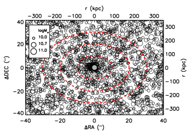
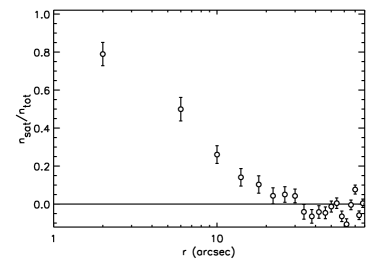
Figure 3: Left: Positions of all satellite candidates (open circles) compared to their respective centrals (filled circle), with the overdensity most visible at $\lesssim 10$″. The size of each symbol varies as a function of its stellar mass. The red dashed contours show scales of 10″, 20″, and 30″, respectively. Right: fraction of expected “real associations” among satellite candidates, $n_{sat}/n_{tot}$ as a function of radius (where $n_{sat}(r)=n(r)-n_{b}$, $n(r)$ and $n_{b}$ being, respectively, the number density of satellite candidates at radius $r$ and at $>50$″).

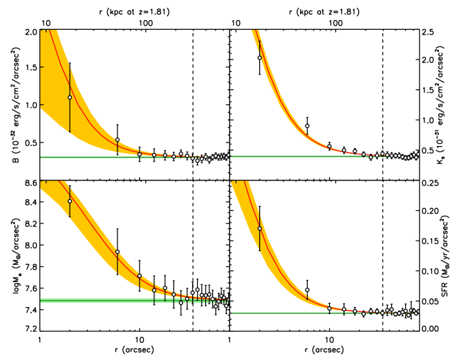
Figure 4: Density profiles of satellites, shown in bins of 4″ ($\sim 35$ kpc at $z\sim 1.8$) for clarity. Clockwise from the top left: $B$- and $K_{s}$-band flux, SFR and stellar mass. The best-fit $\beta$-model, shown with its associated uncertainties by the red line and orange envelope, was derived from the unrebinned data. The dashed vertical line marks the average putative virial radius of the halos and the level of contamination by interlopers (i.e., “background”) is shown in green.

Satellites were grouped in concentric annuli of width 2″ ($\sim 17$ kpc) centered on each halo galaxy, and their relevant properties (photometric fluxes, stellar masses and SFR) averaged in each radial bin. These values were then divided by the total area of the annulus. In each case, the contribution of background and foreground interlopers (hereafter, “background”, for convenience) was estimated from the values in annuli between 50″ and 80″. This region was chosen to be comfortably distant from any significant galaxy excess due to the host halo (as seen in Fig. 3) and cover a large area. We note that this method yields values consistent with background levels determined through random apertures. However, the use of an annular region that is still relatively close to the central should better account for local background variations due to interloper clustering (e.g., galaxy filaments). We use the same background radii for all subsamples and do not attempt to, e.g., adapt the size of the bins to the mass of the central, since $r_{vir}$ is not very sensitive to halo mass variations and the stellar mass scatter of the centrals is consistent with that of a single halo population. Uncertainties in stacked properties were estimated, in each bin, using 1000 bootstrap resamplings of the data, with sizes of half the initial sample. However, bootstrap-derived uncertainties tend to be underestimated as they do not account for systematic uncertainties. This is typically more noticeable in the case of large samples. In an attempt to compensate for it, we rescaled the bootstrap estimates so that, when fitting the background as a constant term, the reduced chi-square be $\chi^{2}_{0}=1$ if initially larger. This is an ad hoc correction meant to produce more conservative error estimates (however, systematic errors are not necessarily Gaussian and the use of a $\chi^{2}$ estimate might not be formally justified). As an example, Fig. 4 shows the averaged stellar mass, SFR, $B-$, and $K_{s}-$band flux density profiles of satellites.

The average number of satellites per central, and the contribution of satellites to the total stellar mass and SFR of the halos, were estimated by fitting a parametric function to the profiles. We have considered both the NFW profile (Navarro, Frenk & White, 1995) and projected $\beta$-model (Cavaliere & Fusco-Femiano, 1978), commonly used for, respectively, dark matter halos and galaxy clusters. We find that the latter provides significantly better agreement ($\Delta$AIC$\sim 45$) with the data, especially at small ($r<5$″) radii where the NFW profile is too shallow. This might be the result of mild mass segregation, as shown in Section 4 (see also, e.g., Watson et al., 2012; van der Burg et al., 2014; Piscionere et al., 2015). On the other hand, the profiles are well fit with $\beta\sim 0.9$. Although a precise constraint of the true shape of the satellite profile is beyond the scope of this paper, this is consistent with values derived at both low and high redshift (e.g., Popesso et al., 2004; Strazzullo et al., 2013). As a check, we have also performed fits letting the background vary freely, which yielded background values consistent with those estimated from the outer annuli.

Integrating the number density profile, we find the average excess of $K_{s}<23.4$ satellites to be $3.3\pm 0.2$. This is somewhat above the value reported by Hartley et al. (2015) for high-redshift centrals and could reflect the different nature of our sample as well as the higher average mass of its centrals. Similarly, we find the integrated stellar mass and SFR of satellites to be M${}_{\star}=(3.6\pm 1)\times 10^{10}$ M_⊙ and SFR $=28\pm 6$ M_⊙ yr^-1, or respectively 28% and 15% of the average central mass and SFR ($1.3\times 10^{11}$ M_⊙ and 192 M_⊙ yr^-1, respectively). However, these values are underestimates for two reasons: first, when selecting satellite candidates, we have considered objects with photometric redshifts consistent with the central’s at only the 68% confidence level. This was done to minimize background contamination when estimating radial profiles and trends (see above and Section 4). However, assuming to the first order that the width of the intrinsic velocity distribution of satellites is negligible compared to photometric errors, and that the background redshift distribution is mostly flat in the redshift range of the selection, we can expect to lose 32% of satellites to redshift uncertainties. The actual integrated mass and SFR should then be higher by a factor of 1.47. Secondly, we have only considered satellites within the completeness limit of the catalog, $K_{s}=23.4$, and thus do not include fainter satellites. At $z\sim 2$, the $K_{s}$ band does not trace stellar mass equally for all galaxies, due to the flux contribution from young stars becoming non-negligible. Through comparison with stellar population models, we have estimated the corresponding mass limits for quiescent and star-forming galaxies to be, respectively, logM_⋆=10.3 and 9.8. The models used here were based on Bruzual & Charlot (2003) templates assuming, respectively, a single burst of maximal age and a main-sequence SFH of the form

$$\textrm{SFR(t)}=10^{-10.2}\times\textrm{M}_{\star}(t)\left(\frac{\textrm{M}_{\star}(t)}{10^{11}\,\textrm{M}_{\odot}}\right)^{-0.2}(1+z(t))^{3}\leavevmode\nobreak\ \leavevmode\nobreak\ \textrm{M}_{\odot}\leavevmode\nobreak\ \textrm{yr}^{-1}$$ (1)

where $M(t)$ and $z(t)$ are, respectively, the stellar mass and redshift at time $t$ after the onset of star formation. The integrated stellar mass of UVJ-selected passive and star-forming satellites were then individually corrected using Tomczak et al. (2014) mass functions (MF) extrapolated to $10^{6}$ M_⊙. A correction to the SFR was similarly estimated, based on the main sequence parametrization shown above. The corrected total stellar mass and SFR are then M${}_{\star,tot,sat}=(9.2\pm 2)\times 10^{10}$ M_⊙ and SFR${}_{tot,sat}=(79\pm 15)$ M_⊙ yr^-1, or respectively $\sim 68$% and $\sim 35$% of the contribution of the central galaxy. Here we have used a “canonical” value of 0.8 for the slope of the main sequence (e.g., Rodighiero et al., 2014). Some recent works, on the other hand, tend to favor a value of near-unity (Abramson et al., 2014; Schreiber et al., 2015). If we assume this value, the corrected SFR value becomes $\sim 54\pm 10$ M_⊙ yr^-1, or $\sim 24$% of the central’s. We note that using Ilbert et al. (2013) MFs, derived on the same field but from a shallower sample, yields very similar values.

3.1 Far-infrared stacks

On the other hand, we have extrapolated the MFs to a mass range where they are not constrained, and for an environment with higher density than the sample from which they were defined. Similarly, the slope of the main sequence at this redshift is mostly unknown below $\sim 10^{9}$ M_⊙. Furthermore, extinction-corrected SED models might still underestimate SFRs in the case of high dust obscuration. The estimated total mass and SFR of satellites are therefore uncertain. As an independent check, we thus also estimated the total SFR of satellites from available FIR maps. Since the resolution of these data (FWHM$\sim 6-20$″) is similar to (or even larger than) the characteristic size of the satellite profile, as seen in Fig. 4, an annulus-based analysis would likely assign a significant fraction of the IR flux emitted by satellites to the central. In addition, satellites close to the mass limit are unlikely to be detected in the relatively shallow Herschel maps, regardless of their separation from the central. To derive the total contribution of satellites to the infrared flux of the halos, we have instead stacked, for each band, 80″$\times$80″ cutout images around each central. These stacked 2D images were then decomposed into a central point source (for the central), a PSF-convolved $\beta$-model centered at the same position (for the satellites) and a constant background term. For this fit, we have used MIPS 24 $\mu$m PSF images based on observations of the GOODS-North field (as used in Elbaz et al., 2011) and Herschel PSFs provided by the PEP and HerMES collaborations. The parameters of the $\beta$-model were fixed to those derived from the catalog-based SFR stack and flux uncertainties were estimated through Monte Carlo simulations based on parameter errors yielded by the fit, after renormalization so that the $\chi^{2}$ be at least one per degree of freedom. Fig. 5 shows the stacked images in the MIPS 24 $\mu$m, Herschel/PACS 100 and 150 $\mu$m, and Herschel/SPIRE 250 and 350 $\mu$m bands, along with the best-fit 2D models and residuals. The decomposition fails in the case of the SPIRE data, yielding only upper limits for the first two bands and providing no meaningful constraint to the 500 $\mu$m flux of satellites. This is likely due to the high confusion limit of the instrument, precluding a straightforward determination of the background (as shown by the residual images in Fig. 5), and to the size of the beam being comparable to or larger than that of the halos themselves.

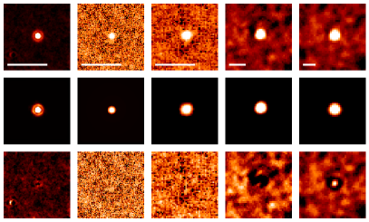
Figure 5: Stacked cutouts (top), best-fit 2D models (middle), and residual images (bottom) from the 24$\mu$m Spitzer/MIPS, 100 and 160$\mu$m Herschel/PACS, 250 and 350$\mu$m Herschel/SPIRE data (left to right; the 500$\mu$m SPIRE image is not shown). The white bar in each top cutout has a length of 30″. We note that in both the cutouts and model images the flux is dominated by the central point-source.

The total infrared luminosity $L_{IR}$ was then derived from the resulting SEDs using Magdis et al. (2012) templates convolved with the redshift distribution of centrals. We have considered both main-sequence and starburst templates, and found that the latter perform significantly worse, as shown in Fig. 6. Converting $L_{IR}$ into SFR assuming the Kennicutt (1998) relation, we find SFR${}_{tot,IR}=176\pm 11$ and $47\pm 6$ M_⊙ yr^-1, for the centrals and satellites respectively, consistent with the values derived from extinction- and completeness-corrected UV SFRs (which we then use in Section 4). We note that the total contribution of satellites is not sufficient to alter the apparent star formation mode (i.e., main-sequence or starburst) of the centrals as determined from the Herschel/PACS data. Finally, we can add to this value the SFR derived from the uncorrected rest-frame UV. Using the $B$-band flux as a measure of the rest-frame 1500$\AA$ emission, this yields $14\pm 3$ and $8\pm 1$ M_⊙ yr^-1 for the satellites and centrals, respectively. The total SFR of satellites estimated from FIR and uncorrected UV is then $60\pm 7$ M_⊙ yr^-1, or $\sim 33$% of the central’s.

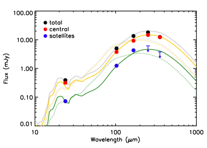
Figure 6: Average far-infrared SED (Spitzer/MIPS 24 $\mu$m, Herschel/PACS 100 and 160 $\mu$m, and Herschel/SPIRE 250 and 350 $\mu$m) of centrals and satellites, with best-fit Magdis et al. (2012) main-sequence templates (solid lines). As comparison, best-fit starburst templates are shown as dotted lines. Both sets of templates have been broadened according to the centrals’ redshift distribution.

3.2 X-ray observations

Since our sample is slightly different and smaller than the one used in Béthermin et al. (2014), the average mass of the host halos studied here might be different from that reported in that paper. As previously, we have used deep X-ray observations of the COSMOS field by the Chandra and XMM-Newton observatories (see, e.g., Finoguenov et al., 2007; Elvis et al., 2009) to constrain the total mass of the halos through a stacking analysis. Of the 215 centrals in the sample, 14 are directly detected as extended sources and 152 are located in zones free from emission. Most of the direct detections appear to be consistent with chance associations along the line of sight with lower-redshift galaxy groups, including 3 that were already known (George et al., 2011). We have accordingly excluded the “direct detections” from the X-ray stack. However, keeping or removing these objects from the sample has no effect on the rest of the analysis presented in this paper and its conclusions. For the sources in regions free from detectable emission, we have used the background-subtracted and exposure-corrected X-ray image, after subtracting detected point sources. The average flux in the 0.5–2 keV band is then $1.1\times 10^{-16}$ erg cm^-2 s^-1, detected at 5.3$\sigma$. Fig. 7 shows a stacked image of these individually undetected objects. For halos in the range $z\sim 1.5-2.5$, using the calibrations of Leauthaud et al. (2010), this flux corresponds to a rest frame 0.1–2.4 keV luminosity of 0.8–2.9$\times 10^{43}$ erg s^-1, an intergalactic medium temperature of $\sim 1$ keV and a total mass of M${}_{200}=2.1-2.4\times 10^{13}$ M_⊙, values similar to those reported in Béthermin et al. (2014). Such sources might then soon be individually detectable in deeper X-ray surveys such as the CDF-S (Finoguenov et al., 2014), where the applicability of the Leauthaud et al. (2010) scaling relations has already been verified for sources with fluxes close to that reported here.

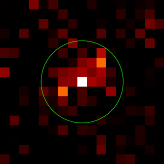
Figure 7: Stacked X-ray image at the position of the centrals (excluding individual detections), from the combined Chandra and XMM-Newton $0.5-2$ keV image of the COSMOS field. For reference, the green circle has a radius of 15″.

3.3 Comparison with model predictions

We have compared the integrated mass and SFR of satellites to the predictions of different halo occupation distribution (HOD) models from Leauthaud et al. (2012), Behroozi et al. (2013), and Béthermin et al. (2013, hereafter, respectively, L12, Bh13 and Bt13). The L12 model is shown for its highest defined redshift bin ($z=0.74-1$) while the last two are both evaluated at $z=1.8$. Fig. 8 shows this comparison for three quantities: the ratio of the total stellar mass of satellites to that of the central, $M_{sat}/M_{cen}$, the fraction of stellar mass (central and satellites) to total mass, $M_{\star}/M_{h}$, and the ratio of the total SFR of satellites to the SFR of the central, SFR${}_{sat}/$SFR_cen. We have here used the total halo masses derived from X-ray stacking, MF-corrected stellar masses and UV+FIR SFRs. All quantities assume the same IMF.

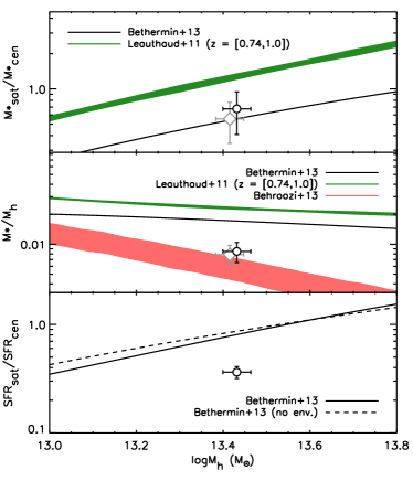
Figure 8: Comparison of the integrated properties of halos in our sample, as a function of halo mass, with model predictions from Béthermin et al. (2013, black), Leauthaud et al. (2012, green), and Behroozi et al. (2013, red): stellar mass fraction of satellites with respect to the central (top), stellar to total mass ratio (middle), and SFR fraction of satellites compared to that of the central (bottom; the dashed line corresponds to a case without environmental effects). The black circle and gray diamond show, respectively, the MF-corrected and uncorrected values. The latter have been shifted to the left for clarity.

The contribution of satellites to the total stellar mass is consistent with the predictions of Bt13 and below L12 at $z\lesssim 1$ (this is to be expected, since $M_{sat}/M_{cen}$ decreases with increasing redshift in both models). We note that this would still be the case if only the measured, uncorrected satellite mass were used. The mass fraction of satellites also appears to be compatible with that predicted at $z=0$ by recent numerical simulations, in the case of $\sim 10^{13}$ M_⊙ halos (Genel et al., 2014; Kravtsov et al., 2014). In our probed mass range, the stellar mass of the central does not evolve much with redshift (Moster et al., 2013; Behroozi et al., 2013), but it is not obvious that this should also be the case for the stellar content of satellites. This might therefore suggest that the processes that determine the baryon conversion efficiency of the host halo also determine to the first order that of the sub-halos. These processes can either act within the host halo (what is usually thought of when considering environmental effects), or in the large-scale structure containing both the central and satellites. In the second case, they would then be related to the conformity of galaxy properties on large scales seen at low redshift (e.g., Park et al., 2008; Ann et al., 2008; Kauffmann et al., 2010, 2013) and help synchronize the stellar mass build-up of the central and its future satellites, before the satellites merge with the host halo.

On the other hand, the measured total stellar mass fraction $M_{\star}/M_{h}$ is somewhat lower than the predictions of Bt13 and more consistent with Bh13. This is not entirely surprising, as the former is optimized to reproduce FIR counts while the latter adopts a more sophisticated treatment of the stellar-to-halo mass relation. The two models also use different stellar mass functions. Furthermore, Fig. 8 does not include the systematic uncertainty on stellar mass estimates ($\sim 0.2-0.3$ dex; see also Section 2). If we take it into account, both the Bt13 and L12 models become compatible with the measured value. Finally, the derived SFR ratio of satellites and centrals is substantially lower than model predictions. This might seem surprising, since the mass ratio is itself fully consistent with expectations. On the other hand, the total SFR of satellites is, in this model, somewhat sensitive to both the behavior of the MF at low masses and the slope of the main sequence. For example, if we assume a slope of unity, instead of the value of 0.8 used by Bt13, the predicted SFR ratio would decrease by a factor of $\sim 2$, making it more consistent with observations. The Bt13 model also adopts a relatively simplified treatment of star formation in sub-halos: in the “no-environment” case, the SFR and the quenched fraction are both a function of sub-halo mass, while in the other case the model assumes that all satellites of active centrals are themselves active. Notably, suppressed (but non-zero) star formation and gradual quenching are not considered.

4 Satellite properties as a function of radius

In this section, we investigate the variation of the stellar population properties of star-forming satellites with distance to the central. As in Section 3, we have selected star-forming satellites based on their rest-frame UVJ colors, using the high-redshift criterion of Williams et al. (2009). Conservatively, we have also excluded nominally star-forming objects that are within 0.1 mag of the dividing line, so as to avoid possible contamination from quiescent satellites. Fig. 9 shows the radial dependency of dust extinction, stellar mass, and specific star formation rate (SFR/M_⋆, or sSFR). We here look at the variation of median values to minimize the effects of outliers. However, because we can expect $\sim 20$% of spurious associations even in the central b in (see Fig. 3), this measure could still be skewed by interloper contamination. To mitigate this, we performed, for each measured quantity, the following statistical background subtraction: in each radial bin within $r_{vir}$, we randomly removed a number of satellite candidates corresponding to the expected number of interlopers, using the background distribution as prior. The uncertainties were estimated from the dispersion of median values of these background-subtracted distributions. To these values, we have added, as in Section 3, the uncertainties derived from bootstrap resampling. This subtraction was performed up to the putative virial radius, although the satellite counts start becoming consistent with background levels already at $r\gtrsim 20$″(or $\sim 170$ kpc; see Fig. 3). For comparison, Fig. 9 also shows the median value prior to the statistical subtraction.

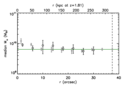
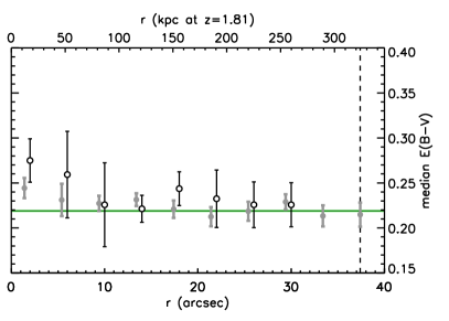
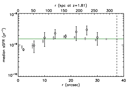
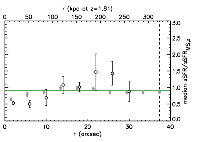
Figure 9: Median background-subtracted stellar population parameters of UVJ-selected star-forming satellites (open symbols), as a function of distance to the central, in bins of 4″: stellar mass (top left), extinction (top right), sSFR (bottom left), and sSFR as a fraction of the main-sequence value (assuming a slope of 0.8). Median values for the total distribution of star-forming satellites (i.e., without subtracting the background distribution) are shown in gray, slightly shifted to the left for convenience. Background levels and related uncertainties, estimated at $r>50$″, are shown in green and the virial radius is indicated by a dashed line.

The stellar mass and extinction of satellites does not vary very much with radius, except in the central bins, where the median M_⋆ and $E(B$-$V)$ are higher than the background value by $\sim 0.2$ dex and $\sim 0.04$ mag, respectively. More surprisingly, while the SFR density of satellites increases monotonously with decreasing halo-centric distance (Fig. 4), their median sSFR varies significantly within the halo, first exhibiting a mild ($\gtrsim 20$%, $\sim 3\sigma$ with respect to the background value) rise at 0.5$r_{vir}$ ($\sim 150$ kpc), then a more significant decrease ($\sim 40$%, $5\sigma$) close to the central ($<50$ kpc). Several interpretations, which we discuss below, could account for this effect.

Normal sSFR variation, as a consequence of the higher median mass of satellites at the center since, in the case of a non-unity slope for the SFR-$M_{\star}$ relation, the sSFR is mass-dependent. However, assuming a slope of $\sim 0.8$ (Rodighiero et al., 2014) and considering the ratio of the sSFR of individual galaxies to that of the main sequence at their stellar mass does not decrease the significance of the sSFR drop at small radii and only slightly that of the excess at $100-200$ kpc (from 3$\sigma$ to 2$\sigma$), as shown in Fig. 9 (bottom right). In fact, a very shallow slope of $\sim 0.3$ would be needed to fully account for the observed sSFR decrease. This value seems unlikely for $\sim 10^{10}$ M_⊙ galaxies at $z\sim 2$ (even in the case of a broken power-law relation; Whitaker et al., 2014) and, in the case of a single power-law, would reinforce the excess at $\gtrsim 150$ kpc. On the other hand, a slope value of near-unity would not alter the shape of the sSFR variation.

Stellar population modeling bias or “missed” SFR from heavily obscured star formation, e.g., due to a systematic underestimation of the extinction-corrected SFR in redder galaxies. We have performed a set of simulations using our stellar population models with varying extinctions and S/N ($E(B$-$V)=0-1$ and S/N$\geq 3$, respectively) to test the first possibility and quantify the bias to stellar population properties in our SED fitting. We find that, when increasing the extinction, faint objects will tend to have their stellar mass underestimated by $\sim 0.05$ dex and their reddening and SFR overestimated by $\sim 0.02$ mag and $\lesssim 10$%, respectively. These values are within the uncertainties of their respective parameters. This is not very surprising, as extinction-corrected SFRs derived from UV-NIR SEDs have already been found to be quite robust (e.g., Rodighiero et al., 2014) and the COSMOS field benefits from a large multiwavelength coverage.

In extreme cases heavily obscured star-forming regions in galaxies could be missed entirely by UV-based estimates. In this scenario, Fig. 9 could then be interpreted as implying a change of star formation mode in satellites as they fall closer to the central, toward heavy obscuration. This would result in a systematic underestimate of the SFR at small radii. Such obscured star formation would however still contribute to the integrated rest-frame near- and far-IR light of the galaxies, and its influence be detectable in broad-band photometry. As shown in Fig. 10 (left), satellites closer to the central galaxy do indeed appear to have slightly redder ($\sim 0.2$ mag) rest-frame $V$-$J$ colors than field galaxies, although the two populations still have compatible $U$-$V$ values and remain within the locus of low-extinction star-forming galaxies. This color difference could be due to a combination of factors, such as longer star formation timescales or higher metallicities (both would increase $(V$-$J)_{0}$ but decrease $(U$-$V)_{0}$) in association with higher ages or extinction (which increase both $(V$-$J)_{0}$ and $(U$-$V)_{0}$). On the other hand, the excellent agreement of the FIR SED of satellites with main-sequence models, and between the FIR and SED-derived total SFRs, suggests that “hidden” star formation is not present in significant quantities (see also Zanella et al., 2015, for similar conclusions).

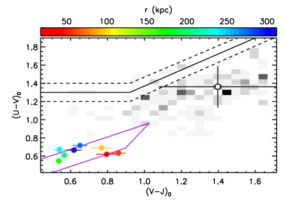
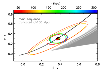
Figure 10: Left: Median rest-frame $U$-$V$ and $V$-$J$ colors, derived from SED modeling, of star-forming satellites (filled circles, colored as a function of distance to the central) and centrals (open circle and gray density histogram). The purple lines show the expected colors of stellar populations models of varying age following a “main-sequence” SFH, assuming $E(B$-$V)<0.3$. Right: median observed $B$-$V$ and $V$-$r$ colors of satellites, as a function of distance to the central, compared to the expected colors of a star-forming model (main-sequence SFH, black) and a constant SFR one observed $\geq 100$ Myr after the quenching of star formation (gray). We here include dust extinction with $E(B$-$V)=0-2$. The ellipses show the dispersion of $B$-$V$ and $V$-$r$ values in each radial bin.

Environmental effect on the activity of satellites, from interaction with the halo and/or the central. In this case, the observed sSFR decrease could originate from two different galaxy populations: systems with non-zero but suppressed star formation, and galaxies where it has recently ceased altogether. As the rest-frame UV bands we have used to select and characterize star formation directly trace the light of massive stars, our estimates are only sensitive to timescales in excess of $100$ Myr (e.g., a galaxy can be expected to stay in the star-forming locus of the UVJ plane for $\sim 300-500$ Myr after cessation of star formation). However, recently quenched systems can be easily distinguished from their still active counterparts due to the aging of their stellar population affecting bluer bands first. Fig. 10 (right), for example, shows two rest-frame UV colors of satellites compared to young stellar population models with and without ongoing star formation. At $z\sim 1.8$ the $B$, $V$, and $r$ filters sample the $1500-2300\AA$ rest-frame and are thus very sensitive to UV light from short-lived massive stars. We see no correlation between the shape of the UV continuum and distance from the central, with satellites at all radii being on average consistent with ongoing star formation.

We therefore conclude that the observed sSFR decrease in UVJ-selected star-forming satellites reflects an actual depression of star formation induced by the group environment. We can estimate a lower limit on the timescale of this effect in the following way: in a pure free-fall case, a galaxy along a radial orbit starting at $r_{vir}$ would reach the center of the halo after $\sim 600-700$ Myr (depending on the concentration of the total matter distribution, if we assume a NFW profile), reaching velocities of $\sim 1000-2000$ km s^-1 and needing only $\sim 100-150$ Myr to cross the last 150 kpc, i.e., the radius corresponding to the observed decrease of sSFR. If we assume, to the first order, that the sSFR drop is due to the absence of gas accretion from the satellites’ reservoirs, and that recycling plays a negligible role, we find (following Erb, 2008) that the time required for the sSFR to decrease to the observed level would indeed be $\lesssim 150$ Myr. This is illustrated in Fig. 11, where we plot, as a function of radius, the diminution of sSFR, assuming the satellites experience no gas infall at $r<150$ kpc. A more circular orbit would increase the time spent by the satellites interacting with the inner halo, while a more gradually diminishing gas supply (as well as some recycling) would also increase the quenching timescale.

Several mechanisms can affect the gas reservoirs of galaxies in dense environments and induce a diminution of star formation (for a review, see, e.g., Boselli & Gavazzi, 2006; Park & Hwang, 2009). Interactions between satellites are here likely not a significant driver of galaxy evolution, as the galaxy density around individual centrals is relatively low. The minimum separation of satellites is $\sim 70-90$ kpc in projection closest to the central (where the signal is dominated by real satellites rather than interlopers; see Fig. 3), an order of magnitude larger than the typical galaxy size in this redshift and mass range (e.g., van der Wel et al., 2014), and already above the scale at which galaxy “harassment” is effective (Moore et al., 1996). Because of the redshift uncertainties for individual satellites, we can expect that the actual distance between them be significantly higher. On the other hand, interaction with the hot diffuse intra-halo gas, whose presence is confirmed by X-ray stacking, constitutes a more plausible source of environmental forcing. The hot gas medium can efficiently shut down star formation, mostly through hydrodynamical interaction, by either preventing further accretion of cold gas onto the galaxies (e.g., “starvation”, Larson et al., 1980; Bekki et al., 2002) or through outright stripping of the galaxies’ interstellar gas (Gunn & Gott, 1972; Nulsen, 1982). These mechanisms are commonly invoked to explain general properties of galaxy populations in clusters, such as systematic sSFR differences with respect to field galaxies (e.g., von der Linden et al., 2010; Alberts et al., 2014) and the lack thereof. In particular, in massive, high-redshift clusters the sSFR of star-forming galaxies does not appear to be much correlated with cluster-centric distance (e.g., Muzzin et al., 2012). This, together with the phase-space distribution of different galaxy populations (Muzzin et al., 2014), is viewed as a sign that the quenching of star formation in dense environments happens on short timescales. The systems studied here probe not only a somewhat higher redshift range than the aforementioned studies, comparable in fact to the current limit of massive cluster samples, but also a mass range that is an order of magnitude lower. They are dynamically simpler than large clusters and with lower velocities, gas temperatures, and densities. The interactions of satellites with their environment should then be less violent. Longer interaction timescales might thus explain the apparent discrepancy between our analysis, which finds a clear sSFR trend, and cluster studies, where such an effect is not seen. On the other hand, in the limit case described above (radial orbit, no gas infall at $\lesssim 150$ kpc), a galaxy falling toward the halo center would have its sSFR decrease by 1 dex in $\sim 1$ Gyr, corresponding to an $e$-folding time of $\sim 0.3$ Gyr. This short timescale is similar to that inferred for massive clusters and consistent with a fast quenching (see also, e.g., Wetzel et al., 2013). While constraining the actual mechanisms acting on the satellites is beyond the scope of this paper and of the data, we note that such timescale is still consistent with either classical “starvation” (i.e., mechanical stripping of the gas reservoir; Bekki et al., 2002) or shock heating of the gas, as predicted by hydrodynamical simulations (here, the interaction between satellites and their host halo would happen at $z<2.5$ in all cases, at an epoch when halos of $\gtrsim 10^{13}$ M_⊙ are expected to be hot and thus prevent efficient cooling of the gas; Dekel & Birnboim, 2006). On the other hand, Ziparo et al. (2013) report no such sSFR gradient in lower redshift groups of similar mass. This might reflect a difference between $10^{13}$ M_⊙ halos at $z\sim 2$ and $z\sim 1$, in timescales for environmental processes or of baryon content. We note however that their highest redshift bin ($1.2<z<1.7$) shows a hint of a $\sim 0.4$ dex sSFR drop similar to what we report here, although it is not significant enough due to the bin containing only one object of uncertain nature (Kurk et al., 2009).

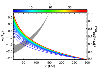
Figure 11: Decrease in sSFR in a simple no-infall, no-recycling case as a function of distance to the center of the halo (gray, right axis; arbitrarily starting at $r=150$ kpc) and tidal perturbation parameter $P_{gc}$ (red to blue, left axis), for a low-mass satellite. The horizontal line shows the threshold value at which the gravitational influence of the halo can trigger inflow within satellite galaxies (Byrd & Valtonen, 1990). Both quantities are shown for NFW concentration parameters ranging from $c=1$ to $c=40$.

On the other hand, the processes described above cannot account for the observed sSFR excess in satellites at $\sim 150$ kpc. We can discount galaxy-galaxy interactions for the same reasons, the median minimum separation of satellites in individual halos being even higher at $>100$ kpc and indistinguishable from field levels. Tidal interaction with the halo, however, by perturbing the gas already in the galaxies, could accelerate star formation in satellites and contribute to clearing their gas (see Valentino et al., 2015, at similar redshift). Following Byrd & Valtonen (1990), we estimate the tidal perturbation parameter $P_{gc}=(M_{h}(r)/M)/(r/A)^{3}$, where $M$, $A$, $r$ and $M_{h}(r)$ are, respectively, the mass and radius of the satellite, its distance from the halo center and the halo mass enclosed within $r$. For $M_{h}(r)$ we assume a NFW profile with a varying concentration in the range $c=1$–40 and a total mass given by the X-ray estimate. We find that in our case the tidal perturbation starts becoming significant ($P_{gc}>0.006$, assuming no stabilizing stellar halo) at a distance of $r<200$ kpc from the halo center, assuming a characteristic satellite mass of $M=7\times 10^{9}$ M_⊙ (see Fig. 2) and size of $A\sim 3$ kpc (van der Wel et al., 2014).

4.1 Passive fraction

Finally, we note that the observed sSFR decrease at small radii is not mirrored by an increase in the number of quiescent satellites near the central. In Fig. 12, we show the ratio of UVJ-selected quiescent satellites to the total number of satellites in each radial bin. We performed the same statistical background subtraction as described above, using the color distributions of the satellites as priors and estimating the quiescent fraction for each random trial. The fraction of quiescent galaxies is close to 20% at large radii and appears to decrease slightly at $r<20$″. This value and trend are similar to those derived by Hartley et al. (2015) from a slightly lower redshift sample. On the other hand, if we adopt a slightly more stringent criterion, by adding a 0.1 mag margin (see Fig. 10) and selecting only the redder UVJ-quiescent galaxies, the background quiescent fraction drops to $\sim$10% and the trend at small radii disappears. This suggests that, at least in our case, it is mostly due to objects close to, or straddling, the dividing line between the passive and star-forming loci. The stellar mass distributions of both quiescent samples are not significantly different, however. The absence of a clear number excess could seem counterintuitive, considering the sSFR variation described in Section 4. On the other hand, the appearance of an obvious quiescent galaxy population takes time. For it to happen in this case, the quenching of star formation in the central satellites would have to have started at $z\sim 2.5$, if we assume a time span of 1 Gyr for a 1 dex sSFR decrease as discussed above. This would in turn imply that the environmental conditions responsible for it (e.g., a hot halo) be already in place at this epoch. We can infer that this was not the case in the type of halos investigated here.

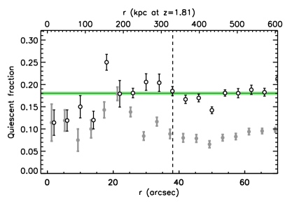
Figure 12: Fraction of quiescent satellites as a function of radius. The satellites were selected according to the UVJ criterion (open symbols), and adding a margin of 0.1 mag in both $(U$-$V)_{0}$ and $(V$-$J)_{0}$ (gray symbols). Values within the virial radius, as shown by the dashed vertical line, were derived from background-subtracted distributions using the same procedure as in Fig. 9. Background levels and related uncertainties, estimated at $r>50$″, are shown in green.

5 Conclusions

Low-mass structures traced by massive galaxies, while more difficult to confirm individually, can be efficiently selected statistically. At high redshift, they can offer a more accessible window to galaxy evolution in dense environments than galaxy clusters, their high abundance compensating for the lower galaxy number density and environmental bias, even in a relatively limited area. We have here taken advantage of the wealth and depth of photometric data available on the COSMOS field to study the distribution and properties of star-forming satellites associated with massive galaxies on the main sequence of star formation, as tracers of group-size halos of mass $\sim 2-3\times 10^{13}$ M_⊙. We have constructed a sample of massive star-forming galaxies at $\langle z\rangle=1.8$, selecting only objects without close neighbors of comparable mass so that they be putatively central to their host halo. We have verified the average total mass of said halos thanks to deep Chandra and XMM data, and found it to be $\lesssim 3\times 10^{13}$ M_⊙. Using the recently released matched photometric catalogs for the COSMOS field, we have derived stellar population parameters for both centrals and satellites. Our conclusions are the following:

• we have estimated the contribution of satellite galaxies to the stellar mass and SFR of the systems at, respectively, $\sim 68$% and $\sim 25-35$% of the stellar mass and SFR of the central galaxy (or $\sim 40$% and $\lesssim 25$% of the total stellar mass and SFR), after correcting for the completeness limit of the sample. The stellar mass fraction of satellites with respect to the central is found to be consistent with the predictions of HOD models, as is the total stellar mass to halo mass ratio. On the other hand, the observed total SFR of satellites appears to be a factor of $\sim 2-3$ lower than model predictions. This might be related to the relatively simple treatment of star formation in sub-halos adopted by our chosen model, or to assumptions on the behavior of the main sequence of star formation at low stellar mass.

• we have also independently estimated the SFR of satellites and centrals from stacked FIR data, by separating their contributions through source decomposition. The SED thus derived is well-fitted by a main-sequence template and yields a SFR of $\sim 47$ M_⊙ yr^-1, consistent with the UV-NIR estimate. This also suggests an absence of significant heavily obscured star formation (e.g., starbursts) in the satellite population.

• finally, we have probed the radial dependence of the properties of star-forming satellites. We find significant variation of their sSFR within the virial radius, with a marginal excess at $r\sim 150$ kpc followed by sharper drop at $r<100$ kpc. This suggests that the group environment acts differently on star-forming galaxies within $r_{vir}$ depending on their distance to the center, enhancing star formation slightly at larger radii while quenching it with a timescale of $\gtrsim 300$ Myr closer to the center. In the first order, this is consistent with destabilization of galactic gas by the halo potential followed by prevention of further gas accretion, as the galaxy falls closer to the center of the halo.

On the other hand, the use of photometric data not only implies some amount of back- and foreground contamination, but also precludes knowledge of important quantities, such as the instantaneous star formation rate and metallicity, that would more precisely constrain the mechanisms of galaxy evolution in these halos. Wide-field, high-coverage spectroscopic instruments (e.g., large integral field units such as MUSE) and, later, “all-in-one” large-scale surveys (e.g., Euclid and WFIRST), should allow for a dramatic improvement in statistics and redshift resolution, especially around the critical epoch of galaxy and cluster progenitor build-up at $z\sim 2$.