The gluing orbit property, uniform hyperbolicity and large deviations principles for semiflows

Abstract.

In this article we introduce a gluing orbit property, weaker than specification, for both maps and flows. We prove that flows with the $C^{1}$-robust gluing orbit property are uniformly hyperbolic and that every uniformly hyperbolic flow satisfies the gluing orbit property. We also prove a level-1 large deviations principle and a level-2 large deviations lower bound for semiflows with the gluing orbit property. As a consequence we establish a level-1 large deviations principle for hyperbolic flows and every continuous observable, and also a level-2 large deviations lower bound. Finally, since many non-uniformly hyperbolic flows can be modeled as suspension flows we also provide criteria for such flows to satisfy uniform and non-uniform versions of the gluing orbit property.

1. Introduction

After the notion of uniform hyperbolicity has been introduced in the seventies by Smale [44], the study of the thermodynamical formalism for uniformly hyperbolic maps and flows has drawn the attention of many researchers. The construction of physical, Sinai-Ruelle-Bowen and equilibrium measures and the study of their statistical properties are some well studied topics. Among the statistical properties, the rates of decay of correlations and large deviations turned out to be much more difficult problem in the time-continuous setting rather than for discrete time dynamics. In fact, while for uniformly hyperbolic diffeomorphisms every Hölder continuous potential admits a unique equilibrium state, which is a Gibbs measure and has exponential decay of correlations (see  [13, 38, 42]) the counterpart of these mixing results for hyperbolic flows was soon proved to be false. Examples of flows that are uniformly hyperbolic but with arbitrarily slow mixing rates were given by Ruelle [39] and later studied by Pollicott [34]. For surveys on mixing rates for hyperbolic flows we refer the reader towards the introductions of [27, 18].

In the nineties, Young, Kifer and Newhouse [53, 24, 25] addressed the question of the velocity of convergence of ergodic averages establishing a connection between the theory of large deviations in probability to the realm of dynamical systems, a topic that has given much description of the chaotic features of dynamical systems. L.-S. Young’s thermodynamical approach to provide large deviations principles for Gibbs measures and all continuous observables usually requires the uniqueness of equilibrium states and some form of specification, which is common among hyperbolic diffeomorphisms. Indeed, every diffeomorphism restricted to a topologically mixing hyperbolic set satisfies the specification property (see e.g. [23]). Other approaches to large deviations whenever the pressure function is differentiable, as the one used by Kifer [24], lead to stronger results although often require observables to be at least Hölder continuous.

For uniformly hyperbolic flows a unified method for large deviations using the thermodynamical approach of [53] and the specification property drops dramatically since uniformly hyperbolic flows may be even not topologically mixing. Nevertheless, Kifer [24] and Waddington [51], among other limit theorems, established a large deviations principle for hyperbolic flows and regular observables (at least Hölder continuous). While good spectral properties of transfer operators imply in other strong consequences, its extension for a broad non-uniformly hyperbolic context usually requires a “case by case” study. To push further the analysis and to be able to consider more general continuous observables, it is natural to introduce other tool that could replace specification as a mechanism to prove large deviations principles. In fact, the recent revived interest for specification properties and large deviations in the last decade shows that the original idea of specification, which corresponds to a strong shadowing of pieces of orbits, introduced by Bowen [11], is far from generating an old fashioned mechanism to study the topological and ergodic features of the dynamical system. While the strong specification property fails to extend beyond uniformly hyperbolic diffeomorphisms and flows (c.f.[45, 46])) many other non-uniform notions have been introduced to reflect non-uniform hyperbolicity (c.f. [35, 33, 50]). In particular one expects the gluing orbit property to be an useful tool to replace the specification property e.g. in the study of multifractal formalism for non-uniformly hyperbolic flows. Just as an illustration the gluing orbit property can be proved to hold for suspension flows over the Manneville-Pomeau. We refer the reader to Section 3 for some examples. A similar notion of gluing for $C^{1}$-diffeomorphisms was introduced in [47], referred as transitive specification property, where the authors prove that this is equivalent to uniform hyperbolicity.

In this paper we shall address on the ergodic theory of semiflows with the gluing orbit property and also provide a characterization of $C^{1}$-smooth flows for which this property holds robustly. One first goal here is to prove large deviations estimates for semiflows with the gluing orbit property. We prove a level-1 large deviations principle for any continuous observable and also prove a level-2 large deviations lower bound for semiflows with the gluing orbit property. In both cases, the estimates and the the rate function are expressed in terms of the thermodynamical quantities and probability measures that invariant either by the time-one map or by the flow (c.f. Theorems D and  E). Since Axiom A flows are semi conjugate to the suspension flows over subshifts of finite type, and these satisty the above mentioned property (as a consequence of Theorem F in Section 2), then a level-1 large deviation principle holds for every transitive hyperbolic flow and every continuous observable. Even in the hyperbolic case our results provide a simpler proof of the level-1 large deviations considered in [51], applies to a wider class of observables and yields a level-2 large deviations lower bound. Let us mention that important level-1 large deviations estimates for non-uniformly hyperbolic flows were obtained e.g. by Melbourne and Nicol [29, 30], Araújo [4] and Araújo and Bufetov [5], where the observables considered are required to have larger regularity than continuity. Most of these results only consider large deviations upper bounds. A second goal here is, in view of the previous discussion, to ask whether if, under some additional conditions, the specification and gluing orbit properties do coincide. Such extra conditions could be from a topological nature (e.g. topological mixing) or on the smooth structure (e.g. the conditions to hold robustly within a $C^{1}$ neighborhood of the original flow). Motivated by the results of Sakai, Sumi, Yamamoto [41] and their extension for flows by Arbieto, Senos, Sodero [6] we prove that $C^{1}$-robustly, the gluing orbit and the specification properties are equivalent to the topological mixing and uniform hyperbolicity of the flow (see Theorem A and Corollary A). Finally, motivated by the fact that many flows can be modeled by suspension semiflows, we prove some criteria for suspension semiflows to satisfy the gluing orbit property.

This article is organized as follows. Definitions and the statement of our main results are given in Section 2. In Section 3 we give some examples to which our results apply while in Section 4 we shall make further comments and discuss some open questions. Section 5 is devoted to the proof of the main results concerning the gluing orbit property and its relation with hyperbolicity. In Section 6 we use the gluing orbit property to provide large deviations upper and lower bounds and establish large deviation principles for flows. In section 7 we provide criteria for such flows satisfy uniform and non-uniform versios of the gluing orbit property. Finally, we include an Appendix where we discuss , for suspension flows, the relation between a tempered variation condition for observables on the manifold and the same condition for the reduced observable on the base dynamics.

2. Preliminaries and Statement of the main results

2.1. Preliminaries

In this section we shall recall some notions that will be necessary for the understanding of our main results and introduce two notions of a gluing orbit property. The reader may decide to skip this section in a first reading and to return to it whenever its makes necessary for the understanding of the article.

2.1.1. Hyperbolic, sectional-hyperbolic and suspension flows

In this subsection we recall some preliminaries on suspension semiflows, uniform and sectional hyperbolicity for flows.

Suspension semiflows

Assume that $M$ be a measurable space and $f$ be a measurable map on $M$. Given an $f$-invariant probability measure $\mu$ and a measurable roof function $\rho\colon M\to[0,+\infty)$ we define the suspension semiflow $(X_{t})_{t\geq 0}$ over $f$ by $X_{t}(x,s)=(x,s+t)$, acting on the quotient space

$$M_{\rho}=\{(x,t)\in M\times\mathbb{R}_{0}^{+}:0\leq t\leq\rho(x)\}/\sim$$

where $\sim$ is the equivalence relation given by $(x,\rho(x))\sim(f(x),0)$. In these coordinates $(X_{t})_{t}$ coincides with the flow consisting in the displacement along the “vertical” direction. If $f$ is invertible and $\rho\in L^{1}(\mu)$ it is not difficult to check that $(X_{t})_{t}$ defines a flow and it preserves the probability measure $\overline{\mu}=(\mu\times\mbox{Leb})/\int\rho\,d\mu,$ where Leb denotes the Lebesgue measure on the real line. Furthermore, observe that $\overline{\mu}$ is uniquely defined by the previous expression provided the roof function $\rho$ is bounded away from zero. Given $\psi:M_{\rho}\rightarrow\mathbb{R}$ we associate the observable $\overline{\psi}:M\rightarrow\mathbb{R}$ defined as $\overline{\psi}(x)=\int_{0}^{\rho(x)}\psi(x,t)dt$. We endow the space $M_{\rho}$ with the Bowen-Walters distance (we refer the reader to the beginning of Section 7 for the precise definition).

Hyperbolic and sectional-hyperbolic flows

Let $M$ be a closed Riemannian manifold, $d$ denote the induced Riemannian distance in $M$, $\|\cdot\|$ the Riemannian norm. Let $(X_{t})_{t}$ be a smooth flow on $M$ and $\Lambda\subseteq M$ be a compact and $(X_{t})_{t}$-invariant set. We say that the flow $(X_{t})_{t}$ to $\Lambda$ is uniformly hyperbolic on $\Lambda$ (or simply that $\Lambda$ is a uniformly hyperbolic set) if there exists a $DX_{t}$-invariant and continuous splitting $T_{\Lambda}N=E^{-}\oplus X\oplus E^{+}$ and constants $C>0$ and $0<\theta_{1}<1$ such that

$$\|DX_{t}\mid E^{-}\|\leq C\theta_{1}^{t}\quad\text{and}\quad\|(DX_{t})^{-1}\mid E^{+}\|\leq C\theta_{1}^{t},\;\forall t\geq 0$$

for every $x\in M$. A flow $(X_{t})_{t}$ is said to be (i) Anosov if the whole manifold $M$ is a hyperbolic set; and (ii) Axiom A if its non-wandering set $\Omega$ is a hyperbolic set with a dense subset of periodic orbits. Uniformly hyperbolic flows have been well studied since the 1970’s and, in particular, their geometric structure is very well understood. It follows from the work of Bowen, Sinai and Ruelle [15, 13, 42] that hyperbolic flows admit finite Markov partitions and that are semi-conjugated to suspension flows over subshifts of finite type.

We say that a $X_{t}$-invariant compact set $\Lambda$ is sectional-hyperbolic if every singularity in $\Lambda$ is hyperbolic and there exist a continuous non-trivial invariant splitting $T_{\Lambda}M=E^{s}\oplus E^{c}$ over $\Lambda$ and constants $C>0$ and $\lambda\in(0,1)$ such that for every $x\in\Lambda$ and $t\geq 0$

• $\|DX_{t}\mid E^{s}_{x}\|\;\|DX_{-t}\mid E^{c}_{X_{t}(x)}\|<C\lambda^{t}$;

• $\|DX_{t}(x)\mid E^{s}_{x}\|\leq C\lambda^{t}$;

• $|\det(DX_{t}(x)\mid_{L_{x}})|>C\lambda^{t}$ for every plane $L_{x}\subset F_{x}$.

We say that $p$ is a hyperbolic critical element if $p$ is either a hyperbolic singularity or a hyperbolic periodic orbit.

2.1.2. Specification and gluing orbit properties

Let us first recall some specification properties in the discrete time setting. We say that a continuous map $f:X\to X$ on a compact metric space $X$ satisfies the specification property if for any $\varepsilon>0$ there exists an integer $N=N(\varepsilon)\geq 1$ such that the following holds: for every $k\geq 1$, any points $x_{1},\dots,x_{k}$, and any sequence of positive integers $n_{1},\dots,n_{k}$ and $p_{1},\dots,p_{k}$ with $p_{i}\geq N(\varepsilon)$ there exists a point $x$ in $M$ such that $\begin{array}[]{cc}d(f^{j}(x),f^{j}(x_{1}))\leq\varepsilon,\end{array}$ for every $0\leq j\leq n_{1}$ and

$$\begin{array}[]{cc}d\big{(}f^{j+n_{1}+p_{1}+\dots+n_{i-1}+p_{i-1}}(x)\;,\;f^{j}(x_{i})\big{)}\leq\varepsilon&\end{array}$$

for every $2\leq i\leq k$ and $0\leq j\leq n_{i}$. Topologically mixing subshifts of finite type are among the class of transformations that satisfy the specification property. Other measure theoretical non-uniform versions of the specification property have been introduced (see e.g. [35, 33, 50]). Following, [50] we say that $(f,\mu)$ satisfies the non-uniform specification property if there exists $\delta>0$ such that for $\mu$-almost every $x$ and every $0<\varepsilon<\delta$ there exists an integer $p(x,n,\varepsilon)\geq 1$ satisfying

$$\lim_{\varepsilon\to 0}\limsup_{n\to\infty}\frac{1}{n}p(x,n,\varepsilon)=0$$

and so that the following holds: given points $x_{1},\dots,x_{k}$ in a full $\mu$-measure set and positive integers $n_{1},\dots,n_{k}$, if $p_{i}\geq p(x_{i},n_{i},\varepsilon)$ then there exists $z$ that $\varepsilon$-shadows the orbits of each $x_{i}$ during $n_{i}$ iterates with a time lag of $p(x_{i},n_{i},\varepsilon)$ in between $f^{n_{i}}(x_{i})$ and $x_{i+1}$, that is,

$$z\in B(x_{1},n_{1},\varepsilon)\quad\text{and}\quad f^{n_{1}+p_{1}+\dots+n_{i-1}+p_{i-1}}(z)\in B(x_{i},n_{i},\varepsilon)$$

for every $2\leq i\leq k.$ Here $B(x,n,\varepsilon):=\{y\in X\colon d(f^{j}(x),f^{j}(y))<\varepsilon,\;\forall j=0\dots n-1\}$ is the usual Bowen ball of length $n$ and size $\varepsilon$ around $x$.

In the context of flows, we say that the flow $(X_{t})_{t\in\mathbb{R}}$ has the specification property on $\Lambda\subset M$ if for any $\varepsilon>0$ there exists a $T=T(\varepsilon)>0$ such that the following property holds: given any finite colection of intervals $I_{i}=[a_{i},b_{i}]$ ($i=1\dots m$) of the real line satisfying $a_{i+1}-b_{i}\geq T(\varepsilon)$ for every $i$ and every map $P:\bigcup_{I_{i}\in\tau}I_{i}\to\Lambda$ such that $X_{t_{2}}(P(t_{1}))=X_{t_{1}}(P(t_{2}))$ for any $t_{1},t_{2}\in I_{i}$ there exists $x\in\Lambda$ so that $d(X_{t}(x),P(t))<\varepsilon$ for all $t\in\bigcup_{i}I_{i}$.

Since the later properties of specification imply on topologically mixing and we need to consider more general transitive dynamics we were led to introduce the following notions.

Definition 2.1.

(Uniform gluing for homeomorphisms) We say a continuous map $f:M\to M$ on a compact metric space $M$ satisfies the gluing orbit property if for any $\varepsilon>0$ there exists an integer $N=N(\varepsilon)\geq 1$ so that for any points $x_{1},x_{2},\dots,x_{k}\in M$ and any positive integers $n_{1},\dots,n_{k}$ there are $p_{1},\dots,p_{k}\leq N(\varepsilon)$ and a point $x$ in $M$ so that $d(f^{j}(x),f^{j}(x_{1}))\leq\varepsilon$ for every $0\leq j\leq n_{1}$ and

$$\begin{array}[]{cc}d\big{(}f^{j+n_{1}+p_{1}+\dots+n_{i-1}+p_{i-1}}(x)\;,\;f^{j}(x_{i})\big{)}\leq\varepsilon&\end{array}$$

for every $2\leq i\leq k$ and $0\leq j\leq n_{i}$.

As mentioned above Axiom A flows are semi-conjugate to suspension flows over subshifts of finite type. Consequently, many important ergodic properties including the thermodynamical formalism of hyperbolic flows can be established using the reduction to the base dynamics (see e.g. [15]). Bowen [12] characterized the Axiom A flows that exhibit the specification property, crucial to deduce lower bound estimates for large deviations using a similar thermodynamical approach to [53], and in particular suspension flows with a roof function cohomologous to a constant never satisfy the specification property. In other words, any Axiom A flow whose stable and unstable manifolds are jointly integrable is not topologically mixing, hence it does not satisfy the specification property (we refer the reader to [12] for more details). Thus we shall consider also a gluing orbit property for semiflows as follows.

Definition 2.2.

(Gluing orbit property for semiflows) Let $(X_{t})_{t\geq 0}$ be a semiflow (not necessarily suspension flow) on a separable metric space $M$. We say that $(X_{t})_{t}$ has the gluing orbit property if for any $\varepsilon>0$ there exists $T(\varepsilon)>0$ so that for any points $x_{1},x_{2},\dots,x_{k}\in M$ and times $t_{1},\dots,t_{k}\geq 0$ there exists $p_{1},\dots,p_{k}\leq T(\varepsilon)$ and $y\in M$ so that

$$d(X_{t}(y)),X_{t}(x_{1}))<\varepsilon\quad\forall t\in[0,t_{1}]$$

and, if $\underline{x}_{i}=X_{\sum_{j=0}^{i-1}p_{j}+t_{j}}(y)\in M$ then

$$d(X_{t}(\underline{x}_{i}),X_{t}(x_{i}))<\varepsilon\quad\forall t\in[0,t_{i}]$$

for every $2\leq i\leq k$. We say the flow $(X_{t})_{t\in\mathbb{R}}$ satisfies the gluing orbit property if the semiflows $(X_{t})_{t\geq 0}$ and $(X_{-t})_{t\geq 0}$ satisfy this property. We let $B(x,t,\varepsilon):=\{y\in X\colon d(X_{s}(x),X_{s}(y))<\varepsilon,\;\forall s\in[0,t]\}$ denote the Bowen ball of size $\varepsilon$ and length $t$ around $x$.

The previous definition roughly means that one can shadow the prescribed pieces of orbits by a real orbit and that the time length needed from one piece to the following can be bounded by some time $T(\varepsilon)$ depending only on the proximity $\varepsilon$. Although the gluing orbit property has the flavor of specification, it is not likely that strong consequences of the later property can be derived under the first much weaker condition. A first evidence is that under the gluing orbit property the dynamical is not necessarily topologically mixing. Finally, notice that the gluing orbit property is clearly a topological invariant.

2.1.3. Tempered distortion and weak Gibbs

In what follows we recall the notions of observables with tempered distortion and the notion of weak Gibbs measures for a flow.

Definition 2.3.

Let $(X_{t})_{t\in\mathbb{R}}$ be a continuous flow on a metric space $M$. We say that a continuous observable $\psi:M\rightarrow{\mathbb{R}}$ has tempered variation if there is $\delta>0$ such that $\lim_{t\to\infty}\frac{1}{t}\gamma(\psi,t,\delta)=0$, where

$$\gamma(\psi,t,\delta):=\sup_{y\in B(x,t,\delta)}\Big{|}\int_{0}^{t}\psi(X_{s}(x))-\psi(X_{s}(y))\;ds\Big{|}.$$

Definition 2.4.

Given a potential $\phi:M\rightarrow{\mathbb{R}}$ and a probability $\mu$, we say that $\mu$ is weak Gibbs with respect to $\phi$, with constant $P_{\mu}\in\mathbb{R}$, if for any $\varepsilon>0$ there exists $K_{t}(\varepsilon)$ (depending only of $\varepsilon$ and of the time $t$) so that $\lim_{t\to\infty}\frac{1}{t}\log K_{t}(\varepsilon)=0$ and

$$\frac{1}{K_{t}(\varepsilon)}\leq\frac{\mu(B(x,t,\varepsilon))}{\exp\Big{[}\int_{0}^{t}\phi(X_{s}(x))ds-tP_{\mu}\Big{]}}\leq K_{t}(\varepsilon)$$ (1)

for every $x\in M$ and $t\in\mathbb{R}$. If $\mu$ is $(X_{t})_{t}$-invariant then $P_{\mu}=h_{\mu}(X_{1})+\int\phi\,d\mu$. If the constants $K_{t}$ can be taken constant independently of the time $t$ then we say that $\mu$ is a Gibbs measure.

2.2. Statement of the main results

We are now in a position to state our main results in which we consider three different directions: (i) relation between the gluing orbit property and uniform hyperbolicity, (ii) large deviations results for semiflows with the gluing orbit property, and (iii) criteria for suspension semiflows to satisfy the gluing orbit properties.

2.2.1. Gluing orbit property from the robust and generic viewpoints

Our purpose here is to compare the gluing orbit property and the specification property for flows. Taking into account that $C^{1}$-robustness of the specification property implies on topologically mixing and uniformly hyperbolic flows (c.f. [6]) one could wonder if the $C^{1}$-robustness of the gluing orbit property is equivalent to the latter one. First we relate this notions with uniform hyperbolicity.

Theorem A.

Let $X\in\mathfrak{X}^{1}(M)$ be so that there exists a $C^{1}$-open open neighborhood $\mathcal{U}\subset\mathfrak{X}^{1}(M)$ of $X$ so that the flow $(Y_{t})_{t\in\mathbb{R}}$ associated to a vector field $Y\in\mathcal{U}$ satisfies the gluing orbit property. Then the vector field $X$ generates a robustly transitive Anosov flow $(X_{t})_{t\in\mathbb{R}}$.

The following is a direct consequence of the previous result, the stability of Anosov flows and that $C^{1}$-robust specification implies topologically mixing Anosov flows (c.f. [6]).

Corollary A.

Let $X\in\mathfrak{X}^{1}(M)$. The following are equivalent:

1. $X$ generates a topologically mixing Anosov flow;

2. $X$ satisfies the $C^{1}$-robust specification property; and

3. $X$ satisfies $C^{1}$-robustly both the topologically mixing and gluing orbit properties.

In view of Corollary A it is natural to ask whether every topologically mixing smooth flow with the gluing orbit property satisfies the specification property. We believe such examples may exist for topologically mixing flows obtained as suspension of beta maps but we do not prove or use this fact here. Finally, following the same lines as in the proof of [6, Theorem 2.6] we can also prove the following:

Theorem B.

There exists a $C^{1}$-residual subset $\mathcal{R}\subset\mathfrak{X}^{1}(M)$ so that any vector field $X\in\mathcal{R}$ satisfying the gluing orbit property generates a transitive Anosov flow.

2.2.2. Large deviations principles

In what follows we will be mostly interested in obtaining lower bound large deviation estimates for semiflows with the gluing orbit property, a problem that revealed difficulties even for uniformly hyperbolic flows. Indeed, although a large deviations principle holds for continuous observables and Axiom A diffeomorphisms using the specification property (see e.g. [53]) a counterpart for flows does not follow immediately for Axiom A flows since typically the strategy for lower bound estimates involve some specification property which occurs only among topologically mixing dynamics. In the mid nineties, Waddington [51] obtained, among other limit theorems, a large deviations principle for weakly topologically mixing Anosov flows. Here we prove a level-1 large deviations principle for every basic piece for an Axiom A flow and any continuous observable, which is a consequence of the following theorem and the existence of the semiconjugacy to symbolic dynamics obtained in [15]. Before stating it precisely just recall the topological pressure of the flow $(X_{t})_{t}$ with respect to the potential $\phi$ is defined by

$$P_{\operatorname{top}}((X_{t})_{t},\phi):=\sup_{\mu\in\mathcal{M}_{X_{1}}}\big{\{}h_{\mu}(X_{1})+\int\phi\,d\mu\big{\}}$$ (2)

and an equilibrium state $\mu_{\phi}$ for $(X_{t})_{t}$ with respect to the potential $\phi$ is a probability measure that attains the supremum.

Theorem C.

Let $\sigma:\Sigma\to\Sigma$ be a subshift of finite type, $\rho:\Sigma\rightarrow{\mathbb{R}}$ be a Hölder continuous roof function and $(X_{t})_{t}$ be the suspension flow associated to $\sigma$ and $\rho$. Let $\phi:\Sigma_{\rho}\to\mathbb{R}$ be a continuous potential so that $\mu_{\phi}$ is an unique equilibrium state for $(X_{t})_{t}$ with respect to $\phi$ and is a Gibbs measure. For any continuous observable $\psi:\Sigma_{\rho}\to\mathbb{R}$ it holds that

$$\limsup_{t\to+\infty}\frac{1}{t}\log\mu_{\phi}\Big{(}x\in\Sigma_{\rho}:\frac{1}{t}\int_{0}^{t}\psi(X_{s}(x))\,ds\in[a,b]\Big{)}\leq-\inf_{s\in[a,b]}I(s)$$

and

$$\liminf_{t\to+\infty}\frac{1}{t}\log\mu_{\phi}\Big{(}x\in\Sigma_{\rho}:\frac{1}{t}\int_{0}^{t}\psi(X_{s}(x))\,ds\in(a,b)\Big{)}\geq-\inf_{s\in(a,b)}I(s)$$

where $I(s)=\sup\{P_{\operatorname{top}}((X_{t})_{t},\phi)-\frac{h_{\eta}(\sigma)}{\int\rho d\eta}-\frac{\int\overline{\phi}\,d\eta}{\int\rho d\eta}:\eta\in\mathcal{M}_{\sigma}\,\&\,\frac{\int\overline{\psi}\,d\eta}{\int\rho d\eta}=s\}$ is the rate function and $\mathcal{M}_{\sigma}$ denotes the space of $\sigma$-invariant probability measures. In particular, if $\bar{\psi}$ is not cohomologous to constant (meaning $\mathcal{M}_{\sigma}\ni\eta\mapsto\int\bar{\psi}d\eta$ is not a constant function) and the interval $[a,b]$ does not contain $\int\psi\,d\mu_{\phi}$ then the right hand sides above are strictly negative.

Let us stress that large deviations lower bounds are much harder to obtain in virtue of the fact that points that are not fastly converging to the mean can generate invariant measures that are not ergodic. It is at this point that some specification-like property is needed. The following result strenghs the proof of usual large deviations lower bounds requiring only the gluing orbit property.

Theorem D.

Let $M$ be a metric space and $(X_{t})_{t}$ be a semiflow satisfying the gluing orbit property. Assume $\phi:M\rightarrow{\mathbb{R}}$ is a bounded potential with tempered variation, $\mu$ is a weak Gibbs probability with respect the $X_{t}$ and $\phi$ with constant $P=P_{\mu}$. Given real numbers $a\leq b$:

• if $\psi:M\rightarrow{\mathbb{R}}$ is a bounded observable with tempered variation then

  $$\liminf_{t\to\infty} \frac{1}{t}\log\mu\Big{(}x\in M:\frac{1}{t}\int_{0}^{t}\psi(X_{s}(x))ds\in(a,b)\Big{)}$$

  $$\geq-\inf\Big{\{}P_{\mu}-h_{\nu}(X_{1})-\int\phi\,d\nu:\nu\text{ is }X_{1}\text{-invariant and }\int\psi\,d\nu\in(a,b)\Big{\}}$$

  $$\geq-\inf\Big{\{}P_{\mu}-h_{\nu}(X_{1})-\int\phi\,d\nu:\nu\text{ is }(X_{t})_{t}\text{-invariant and }\int\psi\,d\nu\in(a,b)\Big{\}}$$

• if $M$ is compact and $\psi:M\rightarrow{\mathbb{R}}$ is continuous then

  $$\limsup_{t\to\infty} \frac{1}{t}\log\mu\Big{(}x\in M:\frac{1}{t}\int_{0}^{t}\psi(X_{s}(x))ds\in[a,b]\Big{)}$$

  $$\leq-\inf\Big{\{}P_{\mu}-h_{\nu}(X_{1})-\int\phi\,d\nu:\nu\text{ is }(X_{t})_{t}\text{-invariant and }\int\psi\,d\nu\in[a,b]\Big{\}}.$$

In fact we can obtain lower bounds for the velocity of convergence of empirical measures to open sets in the space of all probability measures. More precisely,

Theorem E.

Let $(X_{t})_{t}$ be a semiflow on a compact metric space $M$ having the gluing orbit property, $\phi:M\rightarrow{\mathbb{R}}$ be a bounded potential with tempered variation and $\mu$ be a weak Gibbs probability for $X_{t}$ with respect to $\phi$ with constant $P=P_{\mu}$. If $\psi:M\rightarrow{\mathbb{R}}$ is a bounded observable with tempered variation then

$$\liminf_{t\to\infty} \frac{1}{t}\log\mu\Big{(}x\in M:\frac{1}{t}\int_{0}^{t}\delta_{X_{s}(x)}ds\in V\Big{)}$$

$$\geq-\inf\Big{\{}P_{\mu}-h_{\nu}(X_{1})-\int\phi\,d\nu:\nu\text{ is }X_{1}\text{-invariant and }\nu\in V\Big{\}}$$

for any open set $V$ in the space of probability measures on $M$.

Remark 2.5.

Arguments similar to the ones involved in the proof of the previous theorem yield a large deviations principle holds for weak Gibbs measures, bounded observables with tempered variation and discrete time maps with the gluying orbit property, extending [53].

2.2.3. Criteria for gluing orbit properties

In this subsection we provide some criteria for suspension flows to satisfy either the (uniform) gluing orbit property introduced in Subsection 2.1.2 or a non-uniform measure theoretical gluing orbit property.

Theorem F.

Let $M$ be a metric space and let $f:M\rightarrow M$ satisfy the gluing orbit property. Assume the roof function $\rho:M\to\mathbb{R}_{0}^{+}$ is bounded from above and below, is uniformly continuous and the constants

$$C_{\xi}:=\sup_{n\geq 1}\sup_{y\in B(x,n,\xi)}|S_{n}r(x)-S_{n}r(y)|<\infty\quad\text{satisfy }\lim_{\xi\to 0}C_{\xi}=0,$$ (3)

where $S_{n}r=\sum_{j=0}^{n-1}r\circ f^{j}$. Then the suspension semiflow $(X_{t})_{t}$ has the gluing orbit property.

Let us observe that condition (3) is a bounded distortion property for the roof function. It is not hard to check It holds e.g. for Hölder continuous observables and uniformly expanding dynamics. Since the requirement of the theorem on the base dynamics to satisfy a gluing orbit property then the later result applies for suspension flows of transitive but non topologically mixing subshifts of finite type. From the measure theoretical sense the shadowing of pieces of orbits can be actually non-uniform in the following sense.

Definition 2.6.

(Non-uniform gluing) Let $(X_{t})_{t}$ be a semiflow on a separable metric space $M$ and consider a $(X_{t})_{t}$-invariant and ergodic probability measure $\overline{\mu}$. We say that $((X_{t})_{t},\overline{\mu})$ has the non-uniform gluing orbit property if for any $\varepsilon>0$ and for $\overline{\mu}$-almost every point $x\in M$ and $t\geq 0$ there exists $T((x,t,\varepsilon)>0$ so that

$$\lim_{\varepsilon\to 0}\limsup_{t\to+\infty}\frac{T(x,t,\varepsilon)}{t}=0$$

and for $\overline{\mu}^{k}$-almost every points $(x_{1},x_{2},\dots,x_{k})\in M^{k}$ and times $t_{1},\dots,t_{k}\geq 0$ there are $0\leq p_{i}\leq T(x_{i},t_{i},\varepsilon)$ and $x\in M$ satisfying

$$d(X_{t}(x),X_{t}(x_{1}))<\varepsilon\quad\forall t\in[0,t_{1}]$$

and, if $\underline{x}_{i}=X_{\sum_{j=0}^{i-1}p_{j}+t_{j}}(y)\in M$ then $d(X_{t}(\underline{x}_{i}),X_{t}(x_{i}))<\varepsilon,\forall t\in[0,t_{i}]$ for every $2\leq i\leq k$.

The previous property, similar to the gluing orbit property, roughly means that at least for a full measure set of points (with respect to $\overline{\mu}$) one can shadow the prescribed pieces of orbits by a real orbit and that the time length needed from one piece to the following can be bounded by some time $T(x,t,\varepsilon)$ that depends both on the point $x$ and the proximity $\varepsilon$ but that sublinear growth in $t$. Actually the integrability of the roof function is enough to obtain the non-uniform gluing orbit property. This allows to consider e.g. suspension flows over subshifts of countable type (see Section 3).

Theorem G.

Let $M$ be a metric space and assume that $f:M\to M$ satisfies the gluing orbit property and let $\mu$ be an $f$-invariant, ergodic probability measure. Assume the roof function $\rho:M\to\mathbb{R}_{0}^{+}$ is continuous, bounded from below, $\rho\in L^{1}(\mu)$ and the constants

$$C_{\xi}(x):=\sup_{n\geq 1}\sup_{y\in B(x,n,\xi)}|S_{n}r(x)-S_{n}r(y)|<\infty\quad\text{satisfy}\quad\lim_{\xi\to 0}C_{\xi}(x)=0\text{ for $\mu$-a.e. $x$.}$$ (4)

Then the suspension flow $(X_{t})_{t}$ has the non-uniform gluing orbit property with respect to the invariant measure $\overline{\mu}$.

The previous result clearly applies in the case that $f$ is a countable full branch Markov expanding map and any integrable roof function. Finally we prove the following:

Theorem H.

Let $M$ be a compact Riemannian manifold and let $f:M\setminus\mathcal{C}\to M$ be a $C^{1+\alpha}$ local diffeomorphism in the whole manifold $M$ except in a non-degenerate critical/singular set $\mathcal{C}\subset{M}$: there exists $B>0$ such that

1. $\displaystyle{\frac{1}{B}dist(x,\mathcal{C})^{\beta}\leq\frac{\|Df(x)v\|}{\|v\|}\leq B\,dist(x,\mathcal{C})^{-\beta}}$ for all $v\in T_{x}{M}$.

2. For every $x,y\in{M}\setminus\mathcal{C}$ with $dist(x,y)<dist(x,\mathcal{C})/2$ we have

   $${\left|\log\|Df(x)^{-1}\|-\log\|Df(y)^{-1}\|\>\right|\leq\frac{B}{dist(x,\mathcal{C})^{\beta}}dist(x,y)}.$$

Assume that $\mu$ is an $f$-invariant, ergodic and expanding measure and that the roof function $\rho:M\setminus\mathcal{C}\rightarrow\mathbb{R}_{0}^{+}$ is continuous, bounded from below, $\rho\in L^{1}(\mu)$ and the bounded distortion condition (4) holds. Then the suspension flow $(X_{t})_{t}$ has the non-uniform gluing orbit property with respect to the invariant measure $\overline{\mu}$.

The fundamental property used in the proof of the previous theorem is the non-uniform specification property for the invariant measure. Although it is enough to assume the measure to satisfy the non-uniform gluing orbit property we did not state the theorem in such abstract context due to the lack of motivating examples. Thus, an analogous statement is most likely to hold whenever $f$ is a $C^{1+\alpha}$-diffeomorphism and $\mu$ is an $f$-invariant hyperbolic measure.

3. Some examples

In this section we discuss the gluing orbit properties for some classes in both the discrete and the continuous time setting. First we prove that every transitive subshift of finite type satisfies the gluying orbit property.

Example 3.1.

Given $d\geq 1$ and a transition matrix $A\in M_{d\times d}(\{0,1\})$ consider the one-sided subshift of finite type $\sigma:\Sigma_{A}\to\Sigma_{A}$ where $\Sigma_{A}=\{(x_{n})_{n\in\mathbb{N}_{0}}\in\{1,\dots,d\}^{\mathbb{N}_{0}}:A_{x_{n},x_{n+1}=1}\}$ is endowed with the pseudo-distance

$$d((x_{n})_{n},(y_{n})_{n})=2^{-N},\quad\text{where}\;N=\min\{n\geq 0:x_{n}\neq y_{n}\}.$$

and let $\mathcal{P}$ denote the natural partition of $\Sigma_{A}$ in cylinders of size one. Given $\varepsilon>0$ let $N_{\varepsilon}\geq 1$ be the smallest positive integer so that $2^{-N_{\varepsilon}}<\varepsilon$ and consider the partition $\mathcal{Q}_{\varepsilon}=\mathcal{P}^{(N_{\varepsilon})}$ where $\mathcal{P}^{(n)}=\bigvee_{j=0}^{n-1}\sigma^{-j}(\mathcal{P})$ is the dynamically defined partition. If $\mathcal{Q}_{\varepsilon}^{(n)}(x)$ denotes the element of the partition $\mathcal{Q}_{\varepsilon}^{(n)}=\bigvee_{j=0}^{n-1}\sigma^{-j}(\mathcal{Q}_{\varepsilon})$ that contains the point $x$ then for all our purposes the dynamical ball $B_{d}(x,n,\varepsilon)$ can be replaced by the partition element $\mathcal{Q}_{\varepsilon}^{(n)}(x)$. We claim that if $\sigma:\Sigma_{A}\to\Sigma_{A}$ is transitive then it satisfies the gluing orbit property. Recall that $\sigma:\Sigma_{A}\to\Sigma_{A}$ is transitive if and only if for any $i,j\in\{1,\dots,d\}$ there exists $n=n_{i,j}\geq 1$ so that $A^{n}_{i,j}=1$, where $A^{n}=(A^{n}_{i,j})_{i,j=1\dots d}$. Let $\tilde{N}=\max\{n_{i,j}:i,j=1\dots d\}$. Given $\varepsilon>0$ take $p(\varepsilon)=\tilde{N}+N_{\varepsilon}$. Given $x_{1},\dots,x_{k}\in\Sigma_{A}$ and $n_{1},\dots,n_{k}\geq 1$ then it follows from the Markov property for $\sigma$ that $\sigma^{n_{i}}(\mathcal{Q}_{\varepsilon}^{(n_{i})}(x_{i}))=\mathcal{Q}_{\varepsilon}(\sigma^{n_{i}}(x_{i}))$ for every $i=1\dots k$. Set $P_{i}:=\sigma^{N_{\varepsilon}}(\mathcal{Q}_{\varepsilon}(\sigma^{n_{i}}(x_{i})))\in\mathcal{P}$ and let $\hat{P}_{i+1}\in\mathcal{P}$ denote the element of the partition $\mathcal{P}$ containing $x_{i+1}$. Using that $\mathcal{Q}_{\varepsilon}(x_{i+1})\subset\hat{P}_{i+1}\in\mathcal{P}$, by transitivity of $\sigma$, there exists $1\leq p_{i}\leq\tilde{N}$ so that $\sigma^{p_{i}}(P_{i})\supset P_{i+1}\supset\mathcal{Q}_{\varepsilon}(x_{i+1})$ for every $1=1\dots k-1$. This proves the gluing orbit property for $\sigma_{A}$ as claimed.

Indeed, the previous example can be adapted to deal with subshifts of countable type $\sigma:\Sigma\to\Sigma$ with $\Sigma\subset S^{\mathbb{N}}$ and an infinite set $S\subset\mathbb{N}$. These model many non-uniformly hyperbolic dynamical systems. If $\Sigma=S^{\mathbb{N}}$ is the full shift then it is clear it satisfies the specification property. The same arguments as the ones of the previous example yield that subshifts of countable type with the gluing orbit property also include important classes of subshifts as the ones with the so called big image and preimage property (see e.g.  [28]).

Example 3.2.

Let $M$ be a compact Riemannian manifold and $\Lambda\subset M$ be a transitive hyperbolic set for a $C^{1}$ flow $(X_{t})_{t}$. We notice that, via the existence of Markov partitions (see e.g. [15, 13]), the restriction of the flow $(X_{t})_{t}$ to $\Lambda$ is semiconjugated to suspension flow with over a transitive subshit of finite type $\sigma$ and a Hölder continuous roof function $\rho$ bounded away from zero. Since $\sigma$ satisfies the gluing orbit property (c.f. Example 3.1) and every Hölder observable on the shift satisfies the bounded distortion condition (3) it follows from Theorem F that $\Lambda$ has the gluing orbit property. Theorem C yields large deviations principles for the flow with respect to all continuous observables. Theorem E implies on a level-2 large deviations lower bound for hyperbolic flows.

Let us observe that suspension flows over subshifts of countable type, since do not have a compact phase space, are not expected to have the gluing orbit property in general. Theorem G implies that the non-uniform gluing orbit property holds provided the roof function is integrable and satisfies the distortion condition (4).

Example 3.3.

It is well known from the pioneering works of Anosov and Sinai $C^{2}$-Riemannian metrics with strictly negative curvature generate Anosov geodesic flows [1, 2], hence satisfy the gluing orbit property restricted to every transitive subset of the non-wandering set. In the case of non-strictly negative curvature a partial solution has been recently announced by Burns, Climenhaga, Fisher and Thompson [17]. Bessa, Torres and Varandas [8] announced recently that there exists a residual subset of $C^{1}$-metrics with bounded curvature whose geodesic flow satisfies a reparametrized gluing orbit property: for any $\varepsilon>0$ there exists $K=K(\varepsilon)\in\mathbb{R}^{+}$ such that for any points $x_{1},x_{2},\dots,x_{k}\in M$ and times $t_{1},\dots,t_{k}\geq 0$ there are $p_{1},\dots,p_{k}\leq K(\varepsilon)$, a reparametrization $\tau\in\mbox{Rep}(\varepsilon)$ and a point $y\in M$ so that

$$d(X^{\tau(t)}(y)),X^{t}(x_{1}))<\varepsilon\quad\forall t\in[0,t_{1}]$$

and

$$d(X^{\tau(t+\sum_{j=0}^{i-1}p_{j}+t_{j})}(y),X^{t}(x_{i}))<\varepsilon\quad\forall t\in[0,t_{i}]$$

for every $2\leq i\leq k$. By Rep we denote the set of all increasing homemorphisms $\tau\colon{\mathbb{R}}\rightarrow{\mathbb{R}}$, called reparametrizations, satisfying $\tau(0)=0$. Fixing $\varepsilon>0$, we define the set

$$\mbox{Rep}(\varepsilon)=\left\{\tau\in\mbox{Rep}:\left|\frac{\tau(t)}{t}-1\right|<\varepsilon,\,t\in{\mathbb{R}}\right\},$$

of the reparametrizations $\varepsilon$-close to the identity. Let us remark that the reparametrization $\tau$ above satisfies $\tau(t_{1}+p)-\tau(t_{1})\leq(1+\varepsilon)p\leq(1+\varepsilon)K(\varepsilon).$ Hence, the later condition is substantially weaker than specification (since it does not imply topologically mixing) but implies strong transitivity conditions: for any two balls of radius $\varepsilon$ there exists a point whose piece of orbit up to a definite time $(1+\varepsilon)K(\varepsilon)$ (depending only on $\varepsilon$) intersects both balls.

In the following example we shall consider flows with an intermittency phenomenon.

Example 3.4.

Consider $M=[0,1]$ and the Maneville-Pomeau map $f_{\alpha}:[0,1]\to[0,1]$ given by

$$f_{\alpha}(x)=\left\{\begin{array}[]{cl}x(1+2^{\alpha}x^{\alpha})&\mbox{if}\;0\leq x\leq\frac{1}{2}\\ 2x-1&\mbox{if}\;\frac{1}{2}<x\leq 1.\end{array}\right.$$

for $\alpha\in(0,1)$. Since this map is semiconjugated to the full shift on two symbols then it satisfies the specification property. For any roof function $\rho$ satisfying (3) and bounded away from zero the semiflow has the gluing orbit property.

Take $\phi:M_{\rho}\to\mathbb{R}$ smooth observable and the reduced observable $\bar{\phi}:M\to\mathbb{R}$ given by $\bar{\phi}(x)=\int_{0}^{\rho(x)}\phi(X_{s}(x,0))\,ds$. If $\bar{\psi}$ satisfies $\sup\bar{\phi}-\inf\bar{\phi}<\log 2$ there exists a unique equilibrium state $\mu_{\bar{\phi}}$ for $f$ with respect to $\bar{\phi}$ (see e.g. [49]). Furthermore, the unique equilibrium state $\mu:=\mu_{\phi}\times\mbox{Leb}/\int\rho\,d\mu_{\phi}$ for the flow satisfies a large deviations principle for every continuous observable. This is the case e.g. for the potential $\phi=0$ and the corresponding (unique) maximal entropy measure $\mu_{0}$. In the case there are more than one equilibrium state the rate function in the large deviations principle may fail to be strictly convex, in which case the exponential large deviations can fail. For instance, Melbourne and Nicol [30] obtained (upper and lower) polynomial deviation bounds for Hölder continuous observables and the SRB measure of these suspension semiflows.

It is likely that the previous example can be adapted to deal with more general almost-hyperbolic flows (e.g. suspension flows of diffeomorhisms obtained from Anosov diffeomorphisms by isotopy to obtain finitely many indifferent periodic points as in [22]).

4. Some comments and open questions

After introducing this property of gluing, it seems natural not only to verify other examples that do satisfy it but also to explore it as a tool. Similarly to the use of specification as a tool, we expect the gluing orbit property to be an useful tool to derive other applications (e.g. multifractal analysis). Let us also stress that the proof of Theorem F in the stronger context of a bi-Lipschitz homeomorphism $f$ and Hölder continuous roof function $\rho$ can be slightly simplified. This follows from the fact that, under these stronger assumptions, one may make use of the pseudo-metric $d_{\pi}$ instead of the Bowen-Walters distance. Although the gluing orbit property is strictly weaker than the specification property it is an interesting challenge to study their relation. With that purpose we pose the following question:

Question 1: Let $\mathcal{G}$ be the class of $C^{1}$-diffeomorphisms with the gluing orbit property. Is there a topologically large (e.g. open, dense, residual, ..) subset $\mathcal{G}_{1}$ of $\mathcal{G}$ so that every topologically mixing diffeomorphism in $\mathcal{G}_{1}$ satisfies the specification property?

We believe some regularity (e.g. smoothness) of the dynamical system should be necessary for presenting a positve answer to the later question. The results by Bowen [14] and Haydn and Ruelle [40, 21] on the thermodynamical formalism of expansive maps with the specification property and recent extensions by Climenhaga and Thompson [16] motivate the study of the ergodic features of maps with the gluing orbit property.

Question 2: Let $f$ be an expansive map (diffeomorphism or non-critical endomorphism) with the gluing orbit property. Does there exist a finite number of equilibrium states for every regular (e.g. Hölder continuous) potential? Do these have exponential decay of correlations? The associated transfer operator is quasi-compact on the $L^{p}$ spaces?

In the discrete time setting one could hope to obtain a spectral decomposition of the non-wandering set in a finite number of pieces, similar to the one for hyperbolic dynamics, that could guarantee that some power of the dynamics satisfies the specification property for each transitive piece in the decomposition. Since constant reparametrizations of time-continuous dynamics does not change the mixing properties this picture cannot be expected for flows with the gluing orbit property. Some interesting classes of dynamical systems for which decay of correlations and large deviations that still remain not fully understood are billiards and geodesic flows. In virtue of our large deviations results it is natural to ask the following questions:

Question 3: (a) Which billiard flows satisfy the gluing orbit property? Do these include dispersing or Sinai billiards flows? (b) Do “most” geodesic flows satisfy the gluing orbit property?

By Example 3.3 the answer to item (b) in the previous question has partial answers in either lower topologies or whenever some condition is given on the set of points with non-negative curvature. We stress that the notions of non-uniformly gluing and a similar notions of almost gluying (similar to the similar notion from [37]) can probably be used to study large deviations and multifractal analysis (see e.g. [9]). Finally, it is well known from earlier work of Sigmund’s [43] for maps with specification have a rich simplex of invariant probability measures. We refer the reader to the survey by Kwietniak, Lacka and Oprocha [26] for a good account on some recent developments and the study of this simplex for maps with specification like properties. Taking this into account it is natural to ask the following question:

Question 4: What is the “richness” of the simplex of invariant probability measures for dynamics with the gluing orbit property? Which items of Sigmund’s theorem (c.f. Theorem 11 in [26]) still hold for dynamics with the gluing orbit property?

5. The gluing orbit property and uniform hyperbolicity

5.1. Proof of Theorems A and  B

In this section we shall prove that either $C^{1}$-robustly or $C^{1}$-generically, the gluing orbit property implies the flow to be uniformly hyperbolic. The proofs here follow closely the strategy in [6] of proving that the later conditions imply that the flow is a star flow, a condition that is equivalent to uniform hyperbolicity of the flow in the $C^{1}$-topology (we refer the reader to the subsections below for details). The main novelty is to understand how the gluing orbit property can be used to establish the constancy of index among hyperbolic critical elements (c.f. Proposition 5.1 below).

Proof of Theorem A

Our purpose here is to prove that the $C^{1}$-robustness of the gluing orbit property implies on the uniform hyperbolicity of the original flow. The argument follows along the same lines of the strategy to prove that robust specification implies on uniform hyperbolicity, with some extra effort due to the fact that one cannot a priori choose a definite iterate of the flow for which stable and unstable manifolds are long enough to intersect. One key ingredient is to prove that all hyperbolic critical elements are necessarily of the same index, that is, the dimension of its stable bundle in the hyperbolic decomposition (this is the counterpart of [6, Theorem 3.3] in our setting).

Let us introduce some necessary notations. Given a hyperbolic critical element $p$ with hyperbolic decomposition $T_{\mathcal{O}(p)}M=E^{s}\oplus<X>\oplus E^{u}$ (if $p$ is periodic) or $T_{p}M=E_{p}^{s}\oplus E_{p}^{u}$ (if $p$ is a singularity) denote the stable index by $\text{ind}^{s}(p):=\dim E^{s}_{p}$. Given a hyperbolic critical element $p$ and $\varepsilon>0$, the local strong stable manifolds of size $\varepsilon$ at $p$ is given by

$$W^{ss}_{\varepsilon}(p)=\{x\in M\colon d(X_{t}(x),X_{t}(p))\leq\varepsilon\;\text{for every }t\geq 0\}$$

is a smooth submanifold (well defined by uniform hyperbolicity) and set

$$W^{cs}_{\varepsilon}(\mathcal{O}(p))=\bigcup_{t\in\mathbb{R}}W^{ss}_{\varepsilon}(X_{t}(p)).$$

The local strong unstable manifolds $W^{uu}_{\varepsilon}(p)$ of size $\varepsilon$ at $p$ and the submanifold $W^{cs}_{\varepsilon}(\mathcal{O}(p))$ are defined analogously by the corresponding stable manifolds for the reversing time flow $(X_{-t})_{t}$.

Proposition 5.1.

If $p,q$ are hyperbolic critical elements for $X\in\mathfrak{X}^{1}(M)$ and the generated flow $(X_{t})_{t}$ satisfies the $C^{1}$-robust gluing orbit property then $\text{ind}^{s}(p)=\text{ind}^{s}(q)$. Moreover, for any $\varepsilon>0$ there exists $L=L(\varepsilon)>0$ so that $X_{L}(W_{\varepsilon}^{cu}(\mathcal{O}(p)))\cap W_{\varepsilon}^{cs}(\mathcal{O}(q)))\neq\emptyset$ and $X_{L}(W_{\varepsilon}^{cu}(\mathcal{O}(q))))\cap W_{\varepsilon}^{cs}(\mathcal{O}(p)))\neq\emptyset$. In particular $W^{cs}(p)$ and $W^{cu}(q)$ intersect.

Proof.

Let $X\in\mathfrak{X}^{1}(M)$ satisfy the $C^{1}$-robust gluing orbit property and $p,q$ hyperbolic critical elements for $X$. There are three cases to consider, depending on whether the critical elements are periodic orbits or singularities. We recall that the gluing orbit property implies transitivity and, consequently, all periodic points and singularities are of saddle type.

Assume first that $p,q$ are hyperbolic periodic orbits. Take $\varepsilon>0$ and let $L(\varepsilon)>0$ be given by the gluing orbit property. Hence, for any $t>0$ there are $0\leq p_{1}(t)=p_{1}(t,p,q)\leq L(\varepsilon)$ and $z_{t}=z(t,p,q)\in M$ so that

$$d(X_{-s}(z_{t})),X_{-s}(p))<\varepsilon\quad\text{and}\quad d(X_{s}(X_{p_{1}(t)}(z_{t})),X_{s}(q))<\varepsilon$$

for every $s\in[0,t]$. By compactness of $[0,L(\varepsilon)]$ one can take a subsequence $t_{n}\to\infty$ so that $p_{1}(t_{n},p,q)\to\tilde{p}_{1}\in[0,L(\varepsilon)]$ as $n$ tends to infinite. Up to consider a subsequence we may assume also that the sequence $(z(t_{n},p,q))_{n\in\mathbb{N}}$ is convergent to some $z\in M$. This implies that

$$d(X_{-s}(z)),X_{-s}(p))\leq\varepsilon\quad\text{and}\quad d(X_{s}(X_{\tilde{p}_{1}}(z)),X_{s}(q))\leq\varepsilon$$ (5)

for every $s\in\mathbb{R}^{+}$, meaning that $z\in W^{cs}_{\varepsilon}(\mathcal{O}(p))\cap X_{\tilde{p}_{1}}(W^{cu}_{\varepsilon}(\mathcal{O}(q))))$. Since $0<\tilde{p}_{1}\leq L$ and $X_{\tilde{p}_{1}}(W^{cu}_{\varepsilon}(\mathcal{O}(q)))\subset X_{L}(W^{cu}_{\varepsilon}(\mathcal{O}(q)))$ this yields $W^{cs}_{\varepsilon}(\mathcal{O}(p))\cap X_{L}(W^{cu}_{\varepsilon}(\mathcal{O}(q)))\neq\emptyset$. A similar argument (reverting the time) yields $X_{L}(W^{cu}_{\varepsilon}(\mathcal{O}(p)))\cap W^{cs}_{\varepsilon}(\mathcal{O}(q)))\neq\emptyset$.

In the case that $p,q$ are both singularities then $\mathcal{O}(p)=p$ and $\mathcal{O}(q)=q$. Proceeding as before we obtain as in the proof of  (5) we get that there exists $z\in M$ so that $d(X_{-s}(z)),p)<\varepsilon$ and $d(X_{s}(X_{\tilde{p}_{1}}(z)),q)<\varepsilon$ for every $s\in\mathbb{R}^{+}$. This ultimately implies that $X_{L}(W_{\varepsilon}^{uu}(p))\cap W_{\varepsilon}^{ss}(q)\neq\emptyset$. Since $W_{\varepsilon}^{cs}(p)=W_{\varepsilon}^{ss}(p)$ and $W_{\varepsilon}^{cu}(p)=W_{\varepsilon}^{uu}(p)$, and analogous statements hold for $q$ then the proposition follows in this second situation.

The proof of the proposition in the case that $p$ is a periodic orbit and $q$ is a singularity is completely analogous to the previous ones and is left as an exercise to the reader. ∎

Now, to complete the proof of the theorem, assume that $X\in\mathfrak{X}^{1}(M)$ admits a $C^{1}$-open neighborhood $\mathcal{U}\subset\mathfrak{X}^{1}(M)$ of vector fields $Y\in\mathcal{U}$ for which the corresponding flows $(Y_{t})_{t\in\mathbb{R}}$ satisfy the gluing orbit property. Since every flow with the gluing orbit property is necessarily transitive then every $C^{1}$-vector field in $\mathcal{U}$ generates a robustly transitive flow and so all periodic points and singularities are of saddle type.

It is well known that the set of Kupka-Smale flows (i.e. flows whose critical elements are hyperbolic and their stable and unstable manifolds either do not intersect or intersect transversely) is $C^{1}$-generic in $\mathfrak{X}^{1}(M)$ (hence dense in $\mathcal{U}$). In particular, if $X\in\mathcal{U}$ is Kupka-Smale and $p,q$ are hyperbolic critical elements for $X$ such that $\dim W^{cs}(p)+\dim W^{cu}(q)\leq\dim M$ then $W^{cs}(p)\cap W^{cu}(q)=\emptyset$ (see Lemma 3.4 in  [6]). In view of Proposition 5.1 the intersections $W^{cs}(p)\cap W^{cu}(q)\neq\emptyset$ are necessarily non-empty. This implies hyperbolic singularities and hyperbolic periodic orbits for $X$ cannot coexist.

Since for $C^{1}$-generic vector fields the critical elements are dense (c.f. Pugh’s general density theorem, see [36]) the critical elements of $X$ cannot be all singularities, since otherwise the vector field $X$ would be constant to zero, which contradicts the robust transitiveness assumption. Thus $\text{Sing}(X)=\emptyset$ for any $X\in\mathcal{U}$ and that the index of all hyperbolic periodic orbits is constant in a neighborhood of $X$. We will make use of the following perturbation result.

Lemma 5.2.

If $X\in\mathcal{U}$ and a periodic orbit of $X$ is not hyperbolic then there exists a $C^{1}$-arbitrarily close perturbation $Y\in\mathfrak{X}^{1}(M)$ displaying two hyperbolic periodic orbits of different index.

The proof of the previous lemma follows ipsis literis the one of [6, Theorem 4.3] and relies on a version of Franks’ lemma for flows (Lemma 1.3 in [31]). Moreover, since the robust weak specification assumption in [31, Lemma 1.3] is not used for the proof of the previous lemma we shall omit its proof. Now, since all hyperbolic periodic points for vector fields in $\mathcal{U}$ have the same index then it follows from Lemma 5.2 that every vector fields in $\mathcal{U}$ do not admit non-hyperbolic periodic points. On the one hand, by Gan, Wen and Zhu [20], every robustly transitive set which is strongly homogeneous of the same index is sectionally hyperbolic. On the other hand, any sectionally hyperbolic flow without singularities is uniformly hyperbolic (see [19]). This implies that $X$ is a transitive Anosov flow and finishes the proof of Theorem A.

Proof of Theorem B

We claim the existence of a $C^{1}$-residual subset $\mathcal{R}\subset\mathfrak{X}^{1}(M)$ so that any $X\in\mathcal{R}$ with the gluing orbit property generates an Anosov flow. Consider the $C^{1}$-residual subset $\mathcal{R}=\mathcal{R}_{1}\cap\mathcal{R}_{2}$, where $\mathcal{R}_{1}$ denotes the $C^{1}$-residual subset of Kupka-Smale vector fields and $\mathcal{R}_{2}$ denotes the $C^{1}$-residual subset given by Pugh’s general density theorem. Since hyperbolic critical elements are dense and the index of all periodic points is constant (c.f. Proposition 5.1) then every $X\in\mathcal{R}$ admits no singularities. We need the following auxiliary result.

Lemma 5.3.

[6, Lemma 5.1] There exists a residual subset $\mathcal{R}_{3}$ of $\mathfrak{X}^{1}(M)$ so that if $X\in\mathcal{R}_{3}$ is $C^{1}$-approximated by a sequence $(X_{n})_{n}$ such that each $X_{n}\in\mathfrak{X}^{1}(M)$ has two distinct hyperbolic periodic orbits, $p_{n},q_{n}$ with different indices and with $d(p_{n},q_{n})<\varepsilon$, then there exist two distinct hyperbolic periodic points, $p,q$ for $X$ with different indices and with $d(p,q)<2\varepsilon$.

We claim that any $X\in\mathcal{R}\cap\mathcal{R}_{3}$ with the gluing orbit property generates a star flow, that is, there exists an open neighborhood $\mathcal{U}$ of $X$ so that all critical elements of $Y\in\mathcal{U}$ are hyperbolic. Assume, by contradiction, this is not the case. Then, there exists a sequence $X_{n}\to X$ (in the $C^{1}$-topology) and $x_{n}$ a non-hyperbolic critical element for the vector field $X_{n}$. This, together with Lemma 5.2, implies that $X$ can be approximated bt a sequence $(\tilde{X}_{n})_{n}$ of $C^{1}$-vector fields each of which exhibits a pair of periodic points $p_{n},q_{n}$ with different index. By Lemma 5.3, $X$ has two periodic orbits of different index, which contradicts the fact that all periodic points have the same index. This completes the proof of the theorem.

6. From gluing to large deviations

This section is devoted to the proof of our large deviations results (Theorems D,  C and  E).

6.1. Reduction to the Poincaré map

Given a suspension semiflow $(X_{t})_{t\geq 0}$ over a base dynamics $f$ with roof function $\rho$, an $f$-invariant probability measure $\mu$ and an observable $\psi:M_{\rho}\rightarrow{\mathbb{R}}$, consider the reduced observable $\overline{\psi}:M\to\mathbb{R}$ given by $\overline{\psi}(x):=\int_{0}^{\rho(x)}\psi(X_{s}(x))ds$ and the flow invariant probability measure $\bar{\mu}:=\frac{\mu\times\text{Leb}}{\int\rho d\mu}$. The following lemma relates equilibrium states for $(X_{t})_{t}$ with equilibrium states for $f$.

Lemma 6.1.

Let $(X_{t})_{t\geq 0}$ be a suspension semiflow over a continuous map $f:M\to M$ with a roof function $\rho:M\to\mathbb{R}^{+}$ bounded away from zero. Given a potential $\phi:M_{\rho}\to\mathbb{R}$ the following are equivalent:

• $\mu_{\phi}=\mu_{f}\times Leb/\int\rho\,d\mu_{f}$ is an equilibrium state for $(X_{t})_{t}$ with respect to $\phi$

• $\mu_{f}$ is an equilibrium state for $f$ with respect to the potential $\bar{\phi}-P\rho$

where $P=P(\phi)$ denotes the topological pressure of the flow with respect to $\phi$.

Proof.

If $\mu_{\phi}$ is an equilibrium state for $(X_{t})_{t}$ with respect to $\phi$ it follows by equation (2) that

$$h_{\mu_{\phi}}(X_{1})+\int\phi\,d\mu_{\phi}=\sup_{\hat{\eta}\in\mathcal{M}_{1}((X_{t})_{t})}\big{\{}h_{\hat{\eta}}(X_{1})+\int\phi\,d\hat{\eta}\big{\}}=:P(\phi).$$

Since $\rho$ is bounded away from zero there is a map between the space $\{\eta\in\mathcal{M}_{\sigma}:\int\rho\,d\eta<\infty\}$ and the space of $(X_{t})_{t}$ invariant probability measures via the map $\eta\mapsto\hat{\eta}:=\frac{(\eta\times\mbox{Leb})}{\int\rho\,d\eta}.$ It follows from a simple computation and the Abramov formula (see e.g. [48]) that

$$\int\phi\,d\hat{\eta}=\frac{\int\bar{\phi}\,d\eta}{\int\rho\,d\eta}\quad\text{and}\quad h_{\hat{\eta}}(X_{t})=\frac{|t|\,h_{\eta}(f)}{\int\rho\,d\eta}$$ (6)

for every $t\in\mathbb{R}^{+}$ and every $(X_{t})_{t}$-invariant probability measure $\hat{\eta}$. Thus, for any $(X_{t})_{t}$ invariant probability measure $\hat{\eta}$ it holds that

$$0\geq-P(\phi)+h_{\hat{\eta}}(X_{1})+\int\phi\,d\hat{\eta}=\frac{-P(\phi)\,\int\rho\,d\eta+h_{\eta}(f)+\int\bar{\phi}\,d\eta}{\int\rho\,d\eta}$$

which is equivalent to the equation

$$h_{\eta}(f)+\int(\bar{\phi}-P(\phi)\rho)\,d\eta\leq 0$$

for every $f$-invariant probability measure $\eta$. Thus $\hat{\eta}$ is an equilibrium state for $(X_{t})_{t}$ with respect to $\phi$ if and only if $\eta$ is an equilibrium state for $f$ with respect to $\phi-P(\phi)\rho$ and $P_{\operatorname{top}}(f,\bar{\phi}-P(\phi)\rho)=0$. This finishes the proof of the lemma. ∎

Lemma 6.2.

Let $(X_{t})_{t\in\mathbb{R}^{+}}$ be a continuous semiflow a metric space $M$ and let $\psi:M\rightarrow{\mathbb{R}}$ be an observable. Assume that either: (i) $M$ is compact and $\psi$ is continuous, or (ii) $\psi$ has tempered variation. Given $(a,b)\subset{\mathbb{R}}$ and $\varepsilon>0$ there exists $\delta,t_{0}>0$ such that if $\frac{1}{t}\int_{0}^{t}\psi(X_{s}(x))ds\in(a,b)$ and $t\geq t_{0}$ then

$$\frac{1}{t}\int_{0}^{t}\psi(X_{s}(y))\;ds\in(a-\varepsilon,b+\varepsilon)\quad\text{for every }y\in B(x,t,\delta).$$

Proof.

In case (i), since $\psi$ is continuous and $M$ is compact then it is uniformly continuous. Given $\varepsilon>0$ arbitrary let $\delta_{0}>0$ be such that $|\psi(x)-\psi(y)|<\varepsilon$ for every $y\in B(x,\delta_{0})$. Thus, for any $t\geq 0$, $0<\delta<\delta_{0}$ and $y\in B(x,t,\delta)$ it holds that

$$\left|\frac{1}{t}\int_{0}^{t}\psi(X_{s}(y))ds-\frac{1}{t}\int_{0}^{t}\psi(X_{s}(x))ds\right|\leq\frac{1}{t}\int_{0}^{t}|\psi(X_{s}(y))-\psi(X_{s}(x))|ds<\varepsilon,$$

which proves the lemma in this first case. In case (ii), since $\psi$ has tempered variation, for any $\varepsilon>0$ there exists $\delta>0$ and $t_{0}>0$ large such that $\Big{|}\frac{1}{t}\int_{0}^{t}\psi(X_{s}(y))ds-\frac{1}{t}\int_{0}^{t}\psi(X_{s}(x))ds\Big{|}\leq\varepsilon$ for every $t\geq t_{0}$ and $y\in B(x,t,\delta)$. The proof now follows analogously as before. ∎

If $M$ is a compact space, the space $\mathcal{M}(M)$ of probability measures on $M$ endowed with the weak^∗-topology is a compact metrizable space. Given a countable and dense subset $(g_{i})_{i\in\mathbb{N}}$ of continuous observables with $\|g_{i}\|=1$ for every $i\in\mathbb{N}$ consider the metric $\tilde{d}$ on $\mathcal{M}(M)$ given by

$$\tilde{d}(\eta_{1},\eta_{2}):=\sum_{i\in\mathbb{N}}\frac{1}{2^{i}}\big{|}\int g_{i}\,d\eta_{1}-\int g_{i}\,d\eta_{2}\big{|}.$$

Observe that $\tilde{d}$ is invariant by translation (i.e. $\tilde{d}(\eta_{1}+\eta_{3},\eta_{2}+\eta_{3})=\tilde{d}(\eta_{1},\eta_{2})$ for all probabilities $\eta_{1},\eta_{2},\eta_{3}$) and that the function $\tilde{d}(\cdot,\eta)$ is convex for any fixed probability measure $\eta$.

Lemma 6.3.

Let $(X_{t})_{t\in\mathbb{R}}$ be a continuous flow on a compact metric space $M$ and let $\tilde{d}$ be the previously defined metric. Given $\varepsilon>0$ there exists $\delta>0$ such that

$$\tilde{d}\Big{(}\frac{1}{t}\int_{0}^{t}\delta_{X_{s}(y)}ds\;,\;\frac{1}{t}\int_{0}^{t}\delta_{X_{s}(x)}ds\Big{)}<\varepsilon\quad\text{for every $y\in B(x,t,\delta)$ and $t\geq 0$.}$$

Proof.

Since the map $M\ni x\mapsto\delta_{x}$ is uniformly continuous, for any $\varepsilon>0$ there exists $\delta>0$ so that if $d(x,y)<\delta$ then $\tilde{d}(\delta_{x},\delta_{y})<\varepsilon$. Hence, if $y\in B(x,n,\varepsilon)$ we have $\tilde{d}\Big{(}\frac{1}{t}\int_{0}^{t}\delta_{X_{s}(y)}ds\;,\;\frac{1}{t}\int_{0}^{t}\delta_{X_{s}(x)}\;ds\Big{)}\leq\frac{1}{t}\int_{0}^{t}\tilde{d}(\delta_{X_{s}(x)}\,,\,\delta_{X_{s}(y)})\;ds<\varepsilon.$ ∎

The remaining of this section is devoted to two results on distance and entropy approximation of invariant measures by ergodic ones. Recall the entropy of an invariant measure $\mu$ for the flow $(X_{t})_{t\in\mathbb{R}}$ as the entropy $h_{\mu}(X_{1})$ of the time-$1$ map (see e.g. [15]). The first result is a consequence of the ergodic decomposition theorem, whose proof can be found e.g. in [5, Lemma 2.11].

Lemma 6.4.

Let $f:M\to M$ be a continuous map on a metric space $M$. Let $\eta$ be an $f$-invariant probability measure and $\psi,\phi:M\rightarrow{\mathbb{R}}$ be functions in $L^{1}(\nu)$. Given $\varepsilon>0$ there exists $\eta_{1},\ldots,\eta_{n}$ $f$-invariant and ergodic probabilities and $a_{1},\dots,a_{n}>0$, with $\sum_{i=1}^{n}a_{i}=1$, such that (i) $|\int\psi d\eta-\int\psi\;d(\sum_{i=1}^{n}a_{i}\eta_{i})|<\varepsilon$; (ii) $|\int\phi d\eta-\int\phi\;d(\sum_{i=1}^{n}a_{i}\eta_{i})|<\varepsilon$ and (iii) $h_{\eta}(f)\leq\sum_{i=1}^{n}\,a_{i}h_{\eta_{i}}(f))+\varepsilon$

A more general approximation result, from which the later follows immediately and that considers the weak^∗ topology, is as follows:

Lemma 6.5.

Let $f:M\to M$ be a continuous map on a compact metric space $M$. Let $\eta$ be an $f$-invariant probability measure and $\tilde{d}$ be the usual metric in the weak^⋆-topology. Given $\varepsilon>0$ there exists $\eta_{1},\ldots,\eta_{n}$ $f$-invariant and ergodic probabilities and $a_{1},\dots,a_{n}>0$, with $\sum_{i=1}^{n}a_{i}=1$, such that (i) $\tilde{d}(\eta,\sum_{i=1}^{n}a_{i}\eta_{i})<\varepsilon$ and (ii) $h_{\eta}(f)\leq\sum_{i=1}^{n}\,a_{i}h_{\eta_{i}}(f))+\varepsilon$.

Proof.

Let $\eta$ be an $f$-invariant probability measure. By ergodic decomposition theorem and convexity of the entropy function (see e.g. [52]), we can write $\eta=\int\eta_{x}\,d\eta(x)$ and $h_{\eta}(f)=\int h_{\eta_{x}}(f)\,d\eta(x),$ where each $\eta_{x}$ denotes an ergodic component of $\eta$. Take a small finite partition $\mathcal{P}$ of the space $\mathcal{M}(M)$ of invariant probability measures with diameter smaller than $\varepsilon$. Set $n=\#\mathcal{P}$ and $a_{i}=\eta(\{x\in M:\eta_{x}\in P_{i}\})$ for every element $P_{i}$ in $\mathcal{P}$. For every $1\leq i\leq n$ pick an ergodic measure $\eta_{i}=\eta_{x_{i}}\in P_{i}$ satisfying $h_{\eta_{x}}(f)\leq h_{\eta_{i}}(f)+\varepsilon$ for $\eta$-almost every $\eta_{x}\in P_{i}$. Part (i) in the lemma is immediate. On the other hand, (ii) follows because

$$h_{\eta}(f)=\int h_{\eta_{x}}(f)\,d\eta(x)\leq\sum_{i=1}^{n}a_{i}\,h_{\eta_{i}}(f)+\varepsilon=h_{\hat{\eta}}(f)+\varepsilon.$$

Finally, by convexity of the metric $\tilde{d}$ we get

$$\tilde{d}\Big{(}\int\eta_{x}\;d\eta(x),\sum_{i=1}^{n}a_{i}\eta_{i}\Big{)}=\tilde{d}\Big{(}\sum_{i=1}^{n}\int_{P_{i}}\eta_{x}\;d\eta(x),\sum_{i=1}^{n}a_{i}\eta_{i}\Big{)}\leq\varepsilon.$$

This finishes the proof of the lemma. ∎

6.2. Proof of the Theorem D

We prove the upper and lower bounds separately. We will need to recall some necessary notions. Given $t,\varepsilon>0$ we say that a set $E\subset M$ is a $(t,\varepsilon)$-separated set for the flow if $\max_{s\in[0,t]}d(X_{s}(x),X_{s}(y))>\varepsilon$ for any $x\neq y\in E$. We say that $E$ is a maximal $(t,\varepsilon)$-separated set if it is a separated set with maximal cardinality (exist by compactness of $M$). Similarly, given $n\in\mathbb{N}$ and $\varepsilon>0$, a set $E\subset M$ is $(n,\varepsilon)$-separated if $\max_{0\leq j\leq n}d(X_{j}(x),X_{j}(y))>\varepsilon$ for any $x\neq y\in E$.

6.2.1. Upper bound

The proof of the upper bound combines the method for estimating large deviations for the time-$1$ map $X_{1}$, potential $\phi_{1}=\int_{0}^{1}\phi\circ X_{s}\,ds$ and observable $\psi_{1}=\int_{0}^{1}\psi\circ X_{s}\,ds$, with an argument to construct flow invariant measures with pressure at least as large as the pressure of any given $X_{1}$-invariant probability measure. Given $T>0$ let $B_{T}$ denote the set of points $x\in M$ so that $\frac{1}{T}\int_{0}^{T}\psi(X_{s}(x))\in[a,b]$. We observe that

$$\limsup_{T\to\infty}\frac{1}{T}\log\mu(B_{T})=\limsup_{n\to\infty}\frac{1}{n}\log\mu(B_{n})$$

and $B_{n}$ is the set of points $x\in M$ for which $\frac{1}{n}S_{n}\psi_{1}(x)\in[a,b]$, where $S_{n}\psi_{1}=\sum_{j=0}^{n-1}\psi_{1}\circ X_{j}$. If $E_{n}\subset B_{n}$ is a maximal $(n,\varepsilon)$-separated set for the flow then $B_{n}\subset\bigcup_{x\in E_{n}}B(x,n,2\varepsilon)$ and it follows from the Gibbs property  (1) that

$$\mu(B_{n})\leq K_{n}(\varepsilon)e^{-nP_{\mu}}\,\sum_{x\in E_{n}}e^{\int_{0}^{n}\phi(X_{s}(x))\,ds}=K_{n}(\varepsilon)e^{-nP_{\mu}}\,\sum_{x\in E_{n}}e^{S_{n}\phi_{1}(x)}$$

for every $n\geq 1$. Thus

$$\limsup_{n\to\infty}\frac{1}{n}\log\mu(B_{n})\leq-P_{\mu}+\limsup_{n\to\infty}\frac{1}{n}\log Z_{n},$$

where $Z_{n}=\sum_{x\in E_{n}}e^{S_{n}\phi_{1}(x)}$. Now, given $\varepsilon>0$, by uniform continuity of $X_{t}$ for $t\in[0,1]$ there exists $\zeta\in(0,1)$ so that any $(n,\varepsilon)$-separated set for the flow is $(n,\zeta\varepsilon)$-separated set for the time one map $X_{1}$. Thus $E_{n}$ is a $(n,\zeta\varepsilon)$-separated set for the time one map $X_{1}$. Following [53], consider the probability measures $\sigma_{n}$ and $\eta_{n}$ given by

$$\sigma_{n}=\frac{1}{Z_{n}}\sum_{x\in E_{n}}e^{S_{n}\phi_{1}(x)}\,\delta_{x}\quad\text{and}\quad\eta_{n}=\frac{1}{n}\sum_{j=0}^{n-1}(X_{j})_{*}\sigma_{n}.$$

Clearly, any weak^∗ accumulation point $\eta$ of the sequence $(\eta_{n})_{n\in\mathbb{N}}$ is an $X_{1}$-invariant probability measure. Let $\mathcal{P}$ be a partition of $M$ with diameter smaller than $\zeta\varepsilon$ and $\eta(\partial\mathcal{P})=0$. By construction every element of $\mathcal{P}^{(n)}=\bigvee_{j=0}^{n-1}X_{-j}(\mathcal{P})$ contains at most one point of $E_{n}$. Thus

$$H_{\sigma_{n}}(\mathcal{P}^{(n)})-\int S_{n}\phi_{1}\,d\sigma_{n}=\log\Big{(}\sum_{x\in E_{n}}e^{S_{n}\phi_{1}}\Big{)}$$

which, as in the usual proof of the variational principle (c.f.[52, Pages 219-221]), guarantees that

$$\limsup_{n\to\infty}\frac{1}{n}\log\sum_{x\in E_{n}}e^{\sum_{j=0}^{n-1}\phi_{1}(X_{j}(x))}\leq h_{\eta}(f)+\int\phi_{1}\,d\eta.$$

Observe also that $\int\psi_{1}\,d\eta\in[a,b]$ by weak^∗ convergence, because $E_{n}$ is contained in $B_{n}$ and

$$\int\psi_{1}\,d\eta_{n}=\frac{1}{n}\sum_{j=0}^{n-1}\frac{1}{Z_{n}}\sum_{x\in E_{n}}e^{S_{n}\phi_{1}(x)}\psi_{1}(X_{j}(x))\in[a,b].$$

The probability measure $\tilde{\eta}:=\int_{0}^{1}(X_{s})_{*}\eta\,ds$ is clearly flow invariant and each probability measure $(X_{s})_{*}\eta$ is $X_{1}$-invariant with the same entropy as $\eta$. Thus

$$h_{\tilde{\eta}}(X_{1})=\int_{0}^{1}h_{(X_{s})_{*}\eta}(X_{1})\,ds=h_{\eta}(X_{1})\quad\text{and}\quad\int\phi\,d\tilde{\eta}=\int\int_{0}^{1}\phi\circ X_{s}\,ds\,d\eta=\int\phi_{1}\,d\eta.$$

This yields that $h_{\eta}(f)+\int\phi_{1}\,d\eta\leq h_{\tilde{\eta}}(f)+\int\phi_{1}\,d\tilde{\eta}.$ Since $\int\psi\,d\tilde{\eta}=\int\int_{0}^{1}\psi(X_{s}(x))\,d\eta=\int\psi_{1}(x))\,d\eta\in[a,b],$ this finishes the proof of the first part of the theorem.

6.2.2. Lower bound

Set $f=X_{1}$ as the time-1 map of the flow $(X_{t})_{t\in\mathbb{R}}$, $(a,b)\subset\mathbb{R}$ be an open interval and $\phi,\psi$ be bounded observables with tempered variation. Given $t>0$ consider the set

$$D_{t}:=\Big{\{}x\in M:\frac{1}{t}\int_{0}^{t}\psi(X_{s}(x))ds\in(a,b)\Big{\}}.$$

Given any $f$-invariant probability measure $\nu$ satisfying $\int\psi d\nu\in(a,b)$ and $\varepsilon>0$ we claim that there exists $t_{1}>0$ so that

$$\mu(D_{t})\geq\exp t\Big{[}h_{\nu}(X_{1})+\int\phi d\nu-P_{\mu}-\varepsilon]$$

for every $t\geq t_{1}$. Since this claim, together with

$$\inf\Big{\{} P_{\mu}-h_{\nu}(X_{1})-\int\phi\,d\nu:\nu\text{ is }X_{1}\text{-invariant and }\int\psi\,d\nu\in(a,b)\Big{\}}$$

$$\leq\inf\Big{\{}P_{\mu}-h_{\nu}(X_{1})-\int\phi\,d\nu:\nu\text{ is }(X_{t})_{t}\text{-invariant and }\int\psi\,d\nu\in(a,b)\Big{\}},$$

implies the statement of the theorem we are left to prove it.

Fix $\nu$ as above and $\varepsilon>0$ arbitrary. Take $\varepsilon_{0}:=\frac{1}{6}\min\{\varepsilon,|a-\int\psi d\nu|,|b-\int\psi d\nu|\}$ and let $\nu_{1},\ldots,\nu_{n}$ be $X_{1}$-invariant and ergodic probability measures so that $\hat{\nu}=\sum_{i=1}^{n}a_{i}\nu_{i}$ is $\varepsilon_{0}$-approximating $\nu$ in the sense of (i)-(iii) in Lemma 6.4. For any $i=1\dots n$ consider the sets

$$E_{t}^{i}:=\Big{\{}x\in M: \Big{|}\frac{1}{\lfloor a_{i}t\rfloor}\int_{0}^{\lfloor a_{i}t\rfloor}\psi(X_{s}(x))ds-\int\psi d\nu_{i}\Big{|}<\varepsilon_{0}$$

$$\&\Big{|}\frac{1}{\lfloor a_{i}t\rfloor}\int_{0}^{\lfloor a_{i}t\rfloor}\phi(X_{s}(x))ds-\int\phi d\nu_{i}\Big{|}<\varepsilon_{0}\Big{\}},$$

where $\lfloor a_{i}t\rfloor$ denotes the integer part of $a_{i}t$.

Using Birkhoff’s ergodic theorem and that entropy can be computed via separated sets (c.f. [23, 52]), there are $t_{1}>0$, $0<\varepsilon_{1},\varepsilon_{2}\leq\varepsilon_{0}$ and a maximal $(\lfloor a_{i}t\rfloor,\varepsilon_{2})$-separated set $N_{t}^{i}=\{x_{t,1}^{i},\ldots,x_{t,m_{t}^{i}}^{i}\}$ of cardinality $m_{t}^{i}\geq\exp\big{[}\lfloor a_{i}t\rfloor(h_{\nu_{i}}(f)-\varepsilon_{1})\big{]}$ for every $t\geq t_{1}$ and $i=1\dots n$. Up to increase $t_{1}$ if necessary, Lemma 6.2 guarantees that there exists $0<\delta\leq\varepsilon_{2}$ small so that $B(x,t,\delta)\subset D_{t}$ for every $x\in D_{t}$ and $t>t_{1}$.

By construction $N_{t}^{i}$ is a $(\lfloor a_{i}t\rfloor,\delta)$-separated set. We now make use of the gluing orbit property at scale $\frac{\delta}{4}$. Indeed, for any $1\leq j_{i}\leq m_{t}^{i}$, with $i=1,\ldots,n$, by the gluing orbit property one can pick $y\in M$ that shadows the pieces of orbits of the points $x^{1}_{t,j_{1}},x^{2}_{t,j_{2}},\dots,x^{n}_{t,j_{n}}$, for $1\leq j_{i}\leq m_{t}^{i}$ within a distance $\frac{\delta}{4}$, by times $\lfloor a_{i}t\rfloor$ and with jump times $p_{1},\ldots,p_{n-1}\leq T(\frac{\delta}{4})$ between each shadowing segment. Let $Y_{t}$ be the set of all such choices of points $y$. Since $\psi$ has tempered variation we may assume $\delta>0$ is small so that $C_{\delta}(\psi)<\varepsilon_{0}/6$ (recall the definition in equation (3)).

Lemma 6.6.

If $t_{1}>0$ is large then $Y_{t}\subset D_{t+nT(\frac{\delta}{4})}$ for every $t\geq t_{1}$.

Proof.

Take $y\in Y_{t}$ and let $x^{1}_{t,j_{1}},x^{2}_{t,j_{2}},\dots,x^{n}_{t,j_{n}}$ be the points that determined the choice of $y$. Splitting the pieces of the orbit of $y$ up to time $t+nT(\frac{\delta}{4})$ according to its shadowing paths of size $\lfloor a_{i}t\rfloor$ and their complements, and setting $p_{0}=a_{0}=0$, then

$$\int_{0}^{t+nT(\frac{\delta}{4}))}\psi(X_{s}(y))ds =\sum_{i=1}^{n}\int_{0}^{\lfloor a_{i}t\rfloor}\psi(X_{s+\sum_{j=0}^{i-1}(\lfloor a_{j}t\rfloor+p_{j})}(y))\,ds$$

$$+\sum_{i=1}^{n}\int_{\lfloor a_{i}t\rfloor+\sum_{j=1}^{i-1}(\lfloor a_{j}t\rfloor+p_{j})}^{\sum_{j=1}^{i}(\lfloor a_{j}t\rfloor+p_{j})}\psi(X_{s}(y))ds$$

$$+\int_{\sum_{j=1}^{n}(\lfloor a_{j}t\rfloor+p_{j})}^{t+nT(\frac{\delta}{4}))}\psi(X_{s}(y))ds$$

where the first term in the right hand sum differs from $\sum_{i=1}^{n}\int_{0}^{\lfloor a_{i}t\rfloor}\psi(X_{s}(x_{t,j_{i}}^{i}))ds$ by at most $\frac{\varepsilon_{0}}{6}(t+nT(\frac{\delta}{4})))$ by the tempered variation property of $\psi$ and choice of $\delta$. Using that $p_{1},\ldots,p_{n-1}\leq T(\frac{\delta}{4}))$ (with $T(\frac{\delta}{4}))$ independent of $t$) up to consider a larger $t_{1}>0$ the sum of the two last summands in the right hand side is bounded above by $2\|\psi\|_{L^{\infty}}nT(\frac{\delta}{4}))$. Finally, using $|\int\psi d\nu-\int\psi d(\sum_{i=1}^{n}a_{i}\nu_{i})|<\varepsilon_{0}$, $x_{t,j_{i}}^{i}\in E_{t}^{i}$, a simple computation using the tempered variation condition for $\psi$ yields that

$$\frac{1}{\lfloor t+nT(\frac{\delta}{4}))\rfloor}\int_{0}^{t+nT(\frac{\delta}{4}))}\psi(X_{s}(y))ds\in\big{(}\int\psi\,d\nu-\varepsilon_{0},\int\psi\,d\nu+\varepsilon_{0}\big{)}\subset(a,b)$$

for every $t\geq t_{1}$, proving the lemma. ∎

We claim that there exists $C>0$ (depending on the vector field $X$, $n$ and $\delta$) and a subset $\tilde{Y}_{t}\subset Y_{t}$ with cardinality larger or equal to $C\cdot\prod_{i=1}^{n}\exp\big{[}\lfloor a_{i}t\rfloor(h_{\nu_{i}}(f)-\varepsilon_{1})\big{]}$ such that the family of dynamical balls $\{B(y,t+nT(\frac{\delta}{4}),\frac{\delta}{4})\}_{y\in\tilde{Y}_{t}}$ is a disjoint family of subsets of $D_{t+nT(\frac{\delta}{4})}$ for every $t\geq t_{1}$. Recall that each $y\in Y_{t}$ is determined by points $x^{1}_{t,j_{1}},x^{2}_{t,j_{2}},\dots,x^{n}_{t,j_{n}}$ ($1\leq j_{i}\leq m_{t}^{i}$), by the shadowing times $\lfloor a_{i}t\rfloor$ and by gluing times $0\leq p_{1},\ldots,p_{n-1}\leq T(\frac{\delta}{4})$ between each shadowing segment (we also write $p_{i}=p_{i}(y)$ to emphasize these are functions of the underlying points and times). Let $t(\delta,n)>0$ be so that $\max_{s\in[0,n\,t(\delta,n)]}d_{C^{0}}(X_{s},Id)<\frac{\delta}{4}$ and write

$$[0,T(\frac{\delta}{4})]=\bigcup_{s=0}^{N(\delta,n)-1}I_{s}\;\bigcup\;I_{N(\delta,n)}$$ (7)

where $N(\delta,n)=\big{[}\frac{T(\frac{\delta}{4})}{t(\delta,n)}\big{]}$ denotes the integer part of $\frac{T(\frac{\delta}{4})}{t(\delta,n)}$, $I_{s}=[st(\delta,n),(s+1)t(\delta,n)[$ for $0\leq s\leq N(\delta,n)-1$, and the last interval $I_{N(\delta,n)}$ has also size bounded by $t(\delta,n)$ and may be reduced to a point. By the pigeonhole principle (recall (7)), for every $1\leq i\leq n-1$ there exists $0\leq s_{i}\leq N(\delta,n)$ so that the set

$$\tilde{Y}_{t}:=\{y\in Y_{t}\colon\;p_{i}(y)\in I_{s_{i}}\;\text{for every }\;1\leq i\leq n-1\}$$ (8)

has cardinality at least $C\cdot\#Y_{t}$ where $C=\frac{1}{N(\delta,n)^{n-1}}$. The family $\{B(y,t+nT(\frac{\delta}{4}),\frac{\delta}{4})\}_{y\in\tilde{Y}_{t}}$ is disjoint. Indeed, if $y_{1}\neq y_{2}\in\tilde{Y}_{t}$, there are $1\leq i\leq n$ and points $x_{1}\neq x_{2}\in N^{i}_{t}$ so that

$$d(X_{\ell+\sum_{j=0}^{i-1}\lfloor a_{j}t\rfloor+p_{j}(y_{1})}(y_{1}),X_{\ell}(x_{1}))<\frac{\delta}{4}\quad\text{and}\quad d(X_{\ell+\sum_{j=0}^{i-1}\lfloor a_{j}t\rfloor+p_{j}(y_{2})}(y_{2}),X_{\ell}(x_{2}))<\frac{\delta}{4}$$

for $\ell\in[0,\lfloor a_{i}t\rfloor]$. Moreover, as points in $N^{i}_{t}$ are $(\lfloor a_{i}t\rfloor,\delta)$-separated, there exists $s_{i}\in[0,\lfloor a_{i}t\rfloor]$ such that $d(X_{s_{i}}(x_{1}),X_{s_{i}}(x_{2}))>\delta.$ Thus, by triangular inequality and the fact that $\sum_{j=0}^{i-1}|p_{j}(y_{1})-p_{j}(y_{2})|<n\,t(\delta,n)$, we conclude that $d(X_{\tilde{s}_{i}}(y_{1}),X_{\tilde{s}_{i}}(y_{2})>\frac{\delta}{4}$ where $0\leq\tilde{s}_{i}:=s_{i}+\sum_{j=0}^{i-1}\lfloor a_{j}t\rfloor+p_{j}(y_{1})\leq t+nT(\frac{\delta}{4})$. This proves the claim.

Finally, we estimate $\mu(D_{t+nT(\frac{\delta}{4})})$, for every $t\geq t_{1}$. Estimates similar to the ones of the previous lemma yield that $\frac{1}{{t+nT(\frac{\delta}{4})}}\int_{0}^{t+nT(\frac{\delta}{4})}\phi(X_{s}(y))ds\in\Big{(}\int\phi\,d\nu-\varepsilon_{0},\int\phi\,d\nu+\varepsilon_{0}\Big{)}$ for all $t\geq t_{1}$. Thus,

$$\mu(D_{t+nT(\frac{\delta}{4})}) \geq\sum_{y\in\tilde{Y}_{t}}\mu\Big{(}B(y,t+nT(\frac{\delta}{4}),\frac{\delta}{2})\Big{)}$$ (9)

$$\geq\frac{1}{K_{t+nT(\frac{\delta}{4})}(\frac{\delta}{2})}\sum_{y\in\tilde{Y}_{t}}\exp\Big{[}\int_{0}^{t+nT(\frac{\delta}{4})}\phi(X_{s}(y))ds-(t+nT(\frac{\delta}{4})P_{\mu}\Big{]}$$

$$\geq\frac{1}{K_{t+nT(\frac{\delta}{4})}(\frac{\delta}{2})}\#\tilde{Y}_{t}\cdot\exp\Big{[}(t+nT(\frac{\delta}{4}))(\int\phi d\nu-\varepsilon_{0})-(t+nT(\frac{\delta}{4})P_{\mu}\Big{]}$$

$$\geq\frac{C}{K_{t+nT(\frac{\delta}{4})}(\frac{\delta}{2})}\exp\Big{[}\sum_{i=1}^{n}\lfloor a_{i}t\rfloor(h_{\nu_{i}}-\varepsilon_{0})+(t+nT(\frac{\delta}{4}))(\int\phi d\nu-\varepsilon_{0})-(t+nT(\frac{\delta}{4}))P_{\mu}\Big{]}.$$

Since $|h_{\nu}(f)-h_{\sum_{i=1}^{n}a_{i}\nu_{i}}(f)|<\varepsilon_{0}$ and $\lim_{t\to\infty}\frac{1}{t}\log K_{t}(\frac{\delta}{2})=0$, one can take $t_{1}>0$ large so that the claim holds. This completes the proof of the theorem.

6.3. Proof of Theorem E

Since this proof has similar ingredients to the one of Subsection 6.2.2 we shall concentrate on the main differences. Fix an open set $V$ in the space of all probabilities in $M$ and, for $t>0$, consider the set

$$D_{t}:=\Big{\{}x\in M:\frac{1}{t}\int_{0}^{t}\delta_{X_{s}(x)}ds\in V\Big{\}}.$$

Take a $X_{1}$-invariant probability measure $\nu\in V$ and $\varepsilon>0$. We claim that there exists $t_{1}>0$ so that

$$\mu(D_{t})\geq\exp t\Big{[}h_{\nu}(X_{1})+\int\phi d\nu-P_{\mu}-\varepsilon\Big{]}$$

for every $t\geq t_{1}$, which will imply the theorem. Fix $\nu$ as above and $\varepsilon>0$ arbitrary.

Take $0<\hat{\varepsilon}\leq\varepsilon$ be such that $B_{\tilde{d}}(\nu,\hat{\varepsilon})\subset V$ (the ball is taken with respect to the metric $\tilde{d}$) and set $\varepsilon_{0}:=\frac{\hat{\varepsilon}}{6}$. Let $\nu_{1},\ldots,\nu_{n}$ be the $X_{1}$-invariant and ergodic probability measures so that $\hat{\nu}=\sum_{i=1}^{n}a_{i}\nu_{i}$ is $\varepsilon_{0}$-approximating $\nu$ in the sense of (i)-(ii) in Lemma 6.5. By Birkhoff’s ergodic theorem there exists $t_{1}>0$ so that the sets

$$E_{t}^{i}:=\Big{\{}x\in M: \;\tilde{d}\Big{(}\frac{1}{\lfloor a_{i}t\rfloor}\int_{0}^{\lfloor a_{i}t\rfloor}\delta_{X_{s}(x)}ds,\nu_{i}\Big{)}<\varepsilon_{0}$$

$$\&\Big{|}\frac{1}{\lfloor a_{i}t\rfloor}\int_{0}^{\lfloor a_{i}t\rfloor}\phi(X_{s}(x))ds-\int\phi\,d\nu_{i}\Big{|}<\varepsilon_{0}\Big{\}},$$

(where $\lfloor a_{i}t\rfloor$ denotes the integer part of $a_{i}t$) satisfy $\nu_{i}(E_{t}^{i})\geq\frac{1}{2}$ for every $t\geq t_{1}$ and $i=1\dots n$. Again, since entropy can be computed via separated sets (c.f. [23]), up to increase $t_{1}>0$ if necessary, there are $0<\varepsilon_{1},\varepsilon_{2}\leq\varepsilon_{0}$ and a maximal $(\lfloor a_{i}t\rfloor,\varepsilon_{2})$-separated set $N_{t}^{i}=\{x_{t,1}^{i},\ldots,x_{t,m_{t}^{i}}^{i}\}$ of cardinality $m_{t}^{i}\geq\exp\big{[}\lfloor a_{i}t\rfloor(h_{\nu_{i}}(f)-\varepsilon_{1})\big{]}$ for every $t\geq t_{1}$ and $i=1\dots n$. Lemma 6.3 guarantees that there exists $0<\delta\leq\varepsilon_{2}$ so that

$$\tilde{d}\Big{(}\frac{1}{t}\int_{0}^{t}\delta_{X_{s}(y)}ds\;,\;\frac{1}{t}\int_{0}^{t}\delta_{X_{s}(x)}ds\Big{)}<\frac{\varepsilon_{0}}{6}$$

for every $y\in B(x,t,\delta)$. Up to increase $t_{1}$ if necessary, this implies that there exists $0<\delta\leq\varepsilon_{2}$ small so that $B(x,t,\delta)\subset D_{t}$ for every $x\in D_{t}$ and $t>t_{1}$.

We now make use of the gluing orbit property for the scale $\delta>0$. Indeed, for any $1\leq j_{i}\leq m_{t}^{i}$, with $i=1,\ldots,n$, by the gluing orbit property one can pick $y\in M$ that shadows the pieces of orbits of the points $x^{1}_{t,j_{1}},x^{2}_{t,j_{2}},\dots,x^{n}_{t,j_{n}}$, for $1\leq j_{i}\leq m_{t}^{i}$ within a distance $\delta$, by times $\lfloor a_{i}t\rfloor$, respectively, and with jump times $p_{1},\ldots,p_{n-1}\leq T(\delta)$ between each shadowing segment. Denote the set of all such choices of points $y$ as the set $Y_{t}$. Since $\tilde{d}(\cdot,\nu)$ is a convex function then the same ideas as in Lemma 6.6 are enough to prove that $Y_{t}\subset D_{t+nT(\delta)}$ for every $t\geq t_{1}$.

Observe the sets $N_{t}^{i}$ are $(\lfloor a_{i}t\rfloor,\varepsilon_{2})$-separated and $0<\delta<\varepsilon_{2}$. The same argument used in the proof of Theorem D implies that there exists $C>0$ (depending on the vector field $X$, $n$ and $\delta$) and a subset $\tilde{Y}_{t}\subset Y_{t}$ with cardinality larger or equal to $C\cdot\prod_{i=1}^{n}\exp\big{[}\lfloor a_{i}t\rfloor(h_{\nu_{i}}(f)-\varepsilon_{1})\big{]}$ such that the family of dynamical balls $\{B(y,t+nT(\frac{\delta}{4}),\frac{\delta}{4})\}_{y\in\tilde{Y}_{t}}$ is a disjoint family of subsets of $D_{t+nT(\frac{\delta}{4})}$ for every $t\geq t_{1}$ and one can estimate $\mu(D_{t+nT(\frac{\delta}{4})})$ similarly to the proof of Lemma 6.6 (using that $\phi$ has tempered variation and it is bounded):

$$\mu(D_{t+nT(\frac{\delta}{4})}) \geq\sum_{y\in\tilde{Y}_{t}}\mu\Big{(}B(y,t+nT(\frac{\delta}{4}),\frac{\delta}{2})\Big{)}$$ (10)

$$\geq\frac{1}{K_{t+nT(\frac{\delta}{4})}(\frac{\delta}{2})}\sum_{y\in\tilde{Y}_{t}}\exp\Big{[}\int_{0}^{t+nT(\frac{\delta}{4})}\phi(X_{s}(y))ds-(t+nT(\frac{\delta}{4}))P_{\mu}\Big{]}$$

$$\geq\frac{1}{K_{t+nT(\frac{\delta}{4})}(\frac{\delta}{2})}\#\tilde{Y}_{t}\cdot\exp\Big{[}(t+nT(\frac{\delta}{4}))(\int\phi d\nu-\varepsilon_{0})-(t+nT(\frac{\delta}{4}))P_{\mu}\Big{]}$$

$$\geq\frac{C}{K_{t+nT(\frac{\delta}{4})}(\frac{\delta}{2})}\exp\Big{[}\sum_{i=1}^{n}\lfloor a_{i}t\rfloor(h_{\nu_{i}}-\varepsilon_{0})+(t+nT(\frac{\delta}{4}))(\int\phi d\nu-\varepsilon_{0})-(t+nT(\frac{\delta}{4}))P_{\mu}\Big{]}.$$

This proves the claim since $|h_{\nu}(f)-h_{\sum_{i=1}^{n}a_{i}\nu_{i}}(f)|<\varepsilon_{0}$ and $\lim_{t\to\infty}\frac{1}{t}\log K_{t}(\frac{\delta}{2})=0$.

6.4. Proof of Theorem C

Let $\sigma:\Sigma\to\Sigma$ be a subshift of finite type, $\rho:\Sigma\rightarrow{\mathbb{R}}$ be a Hölder continuous roof function and $(X_{t})_{t}$ be the suspension flow generated by $\sigma$ and $\rho$. Assume $\phi:\Sigma_{\rho}\to\mathbb{R}$ is a continuous potential so that $\mu_{\phi}$ is the unique equilibrium state for $(X_{t})_{t}$ with respect to $\phi$ and is a Gibbs measure. Applying the Theorem F we have that $(X_{t})_{t}$ has the gluing orbit property. So, by compactness of $\Sigma_{\rho}$ and continuity of the observable $\psi:\Sigma_{\rho}\to\mathbb{R}$ it follows from Theorem D the following level-1 large deviations principle

$$\limsup_{t\to+\infty}\frac{1}{t}\log\mu_{\phi}\Big{(}x\in\Sigma_{\rho}:\frac{1}{t}\int_{0}^{t}\psi(X_{s}(x))\,ds\in[a,b]\Big{)}\leq-\inf_{s\in[a,b]}I(s)$$

and

$$\liminf_{t\to+\infty}\frac{1}{t}\log\mu_{\phi}\Big{(}x\in\Sigma_{\rho}:\frac{1}{t}\int_{0}^{t}\psi(X_{s}(x))\,ds\in(a,b)\Big{)}\geq-\inf_{s\in(a,b)}I(s)$$

with $I(s)=\sup\{P_{\mu}-h_{\nu}(X_{1})-\int\phi\,d\nu:\nu\text{ is }(X_{t})_{t}\text{-invariant and }\int\psi\,d\nu=s\}$. Finally, we observe that for every $(X_{t})_{t}$-invariant probability measure $\nu$ there exists a unique $\sigma$-invariant probability measure so that $\nu=(\eta\times\mbox{Leb})/\int\rho\,d\eta$ (see e.g. [15]). By the Abramov formulas we get

$$h_{\nu}(X_{1})=\frac{h_{\eta}(\sigma)}{\int\rho d\eta}\quad\text{and}\quad\int\phi\,d\nu=\frac{\int\overline{\phi}\,d\eta}{\int\rho d\eta}$$

and, using that $\mu$ is an equilibrium state for $\phi$, it follows that $P_{\mu}=P_{\operatorname{top}}((X_{t})_{t},\phi)$. This finishes the proof of the theorem.

7. Criteria for gluying orbit properties

7.1. The Bowen-Walters distance

Before proving the criteria for suspension semiflows to satisfy gluying orbit properties we recall the Bowen-Walters distance for the suspension semiflows. Assume that $(M,d)$ is a metric space, $f:M\to M$ is a continuous map, $\rho:M\to\mathbb{R}^{+}_{0}$ is a roof function and $(X_{t})_{t\geq 0}$ is the suspension semiflow over $f$ acting on the space $M_{\rho}$ introduced in Subsection 2.1. If $\rho\equiv 1$ is constant equal to one then define a horizontal distance for points in $M\times\{t\}$ by

$$d_{h}((x,t),(y,t))=(1-t)d(x,y)+td(f(x),f(y))$$

and a define a vertical distance for points for $(x,t)$ in the orbit of $(y,s)$ by

$$d_{v}((x,t),(y,s))=\inf\{|r|\colon X_{r}(x,t)=(y,s)\}.$$

Then, the Bowen-Walters distance $d_{1}((x,t),(y,s))$ is defined as the infimum of the length of paths connecting $(x,t)$ and $(x,s)$. For an arbitrary roof function $\rho$ the Bowen-Walters distance is defined, for every $(x,t),(x,s)\in M$, by

$$d_{\rho}((x,t),(x,s)):=d_{1}((x,t/\rho(x)),(y,s/\rho(y))).$$

Although this is a very natural metric, it is also hard to explicitly compute balls and dynamical balls with respect to Bowen-Walters distance. If $f$ is invertible with both $f$ and $f^{-1}$ Lipschitz, and the roof function $\rho$ is bounded away from zero and also Lipschitz continuous then it follows from Barreira and Saussol  [7, Appendix] that there exists $K>0$ so that

$$K^{-1}d_{\pi}((x,t),(y,s))\leq d_{\rho}((x,t),(x,s))\leq Kd_{\pi}((x,t),(y,s))$$ (11)

for any $(x,t),(y,s)\in M$, where $d_{\pi}$ is the pseudo-distance

$$d_{\pi}((x,t),(y,s))=\min\Bigg{\{}\begin{array}[]{l}d(x,y)+|s-t|,\\ d(f(x),y)+\rho(x)-t+s,\\ d(x,f(y))+\rho(y)-s+t\end{array}\Bigg{\}}.$$ (12)

7.2. Proof of Theorem F

Assume that $f:M\to M$ satisfies the gluing orbit property and that the roof function $\rho:M\to\mathbb{R}_{0}^{+}$ is bounded above and below. Let $\varepsilon>0$ be arbitrary and fixed. Take points $(x_{1},s_{1}),(x_{2},s_{2}),\dots,(x_{k},s_{k})\in M_{\rho}$ and times $t_{1},\dots,t_{k}\geq 0$ arbitrary. Given any $1\leq i\leq k$, let $n_{i}=n_{i}(x_{i},s_{i},t_{i})\in\mathbb{N}_{0}$ be determined by the equation

$$\sum_{j=0}^{n_{i}-1}\rho(f^{j}(x_{i}))\leq s_{i}+t_{i}<\sum_{j=0}^{n_{i}}\rho(f^{j}(x_{i})).$$ (13)

Using that $\rho$ is uniformly continuous and satisfies condition (3), there exists $0<\xi<\varepsilon/3$ be small so that $\xi+C_{\xi}<\frac{\varepsilon}{3}$, that $C_{\xi}<\frac{\varepsilon}{3}\inf_{x\in M}\rho(x)$ and $|\rho(z)-\rho(w)|<\frac{\varepsilon(\inf\rho)^{2}}{3\sup\rho}$ for all $d(z,w)<\xi$.

Now we shall use the gluing orbit property for $f$ with the proximity $\xi$. More precisely, if $N(\xi)$ is given by the gluing orbit property for $f$ then there exists $x\in M$ that shadows the pieces of the orbits of the points $x_{i}$ during $n_{i}+1$ iterates with a time lag of at most $N(\xi)$ iterates. More precisely, there are $\tilde{p}_{i}\leq N(\xi)$, $1\leq i\leq k$, and $x\in M$ so that $d(f^{j}(x),f^{j}(x_{1}))\leq\xi$ for every $0\leq j\leq n_{1}+1$ and $d(f^{j+n_{1}+\tilde{p}_{1}+\dots+n_{i-1}+\tilde{p}_{i-1}+(i-1)}(x)\,,\,f^{j}(x_{i}))\leq\xi$ for every $2\leq i\leq k$ and $0\leq j\leq n_{i}+1$. Choose $T(\varepsilon):=T(\xi)=(N(\xi)+2)\,\sup\rho$. Observe that $T(\xi)$ depends only on $\xi$ (hence only depending on $\varepsilon$) and the upper bound for the roof function. Set $s=s_{1}$.

Before giving the full details of the proof let us make some comments to illustrate the difficulties involved. The proof of the theorem consists of proving that the trajectory of the point $(x,s)$ under the action of the suspension semiflow follows closely the pieces of orbit of the prescribed points $(x_{i},s_{i})$ with a control on the time in between. At each moment of the shadowing process one needs a control on the lap number involving either the point $x$ or the points $x_{i}$. Since the lap number corresponding to $x$ and the one for some $x_{i}$ may differ by one, there are at most $18^{k-1}$ cases to consider. We will explicit the key estimates in the case where $k=2$, which encloses all the difficulties of the general case and where the notation is greatly simplified. The general case involves a completely analogous but much more technical computation using the ideas from the case $k=2$. For that purpose, in the remaining we will prove the following:

Claim: $d_{\rho}(X_{t}({x},s),X_{t}(x_{1},s_{1}))<\varepsilon$ for every $t\in[0,t_{1}]$ and there exists $0\leq p_{1}\leq T(\varepsilon)$ so that $d_{\rho}(X_{t+t_{1}+p_{1}}({x},s_{1}),X_{t}(x_{2},s_{2}))<\varepsilon$ for every $t\in[0,t_{2}]$.

Since $s=s_{1}$, for every $t\in[0,t_{1}]$ one can write

$$X_{t}(x,s_{1})=\Big{(}f^{j}(x),s_{1}+t-\sum_{j=0}^{j-1}\rho(f^{j}(x))\Big{)}$$

and

$$X_{t}(x_{1},s_{1})=\Big{(}f^{j_{1}}(x_{1}),s_{1}+t-\sum_{j=0}^{j_{1}-1}\rho(f^{j}(x_{1}))\Big{)},$$

where $j=j(x,s_{1},t)\in\mathbb{N}_{0}$ and $j_{1}=j_{1}(x_{1},s_{1},t)\in\mathbb{N}_{0}$ are uniquely determined by

$$\sum_{i=0}^{j-1}\rho(f^{i}(x))\leq s_{1}+t<\sum_{i=0}^{j}\rho(f^{i}(x))\quad\text{and}\quad\sum_{i=0}^{j_{1}-1}\rho(f^{i}(x_{1}))\leq s_{1}+t<\sum_{i=0}^{j_{1}}\rho(f^{i}(x_{1})).$$ (14)

By the choice of $\xi$ it follows that $C_{\xi}\ll\inf_{x\in M}\rho(x)$ and so $|j(x,s_{1},t)-j_{1}(x,s_{1},t)|\leq 1$ for every $t\in[0,t_{1}]$. Fix $t\in[0,t_{1}]$. We can estimate the $d_{\rho}$-distance according to the following three prototypical cases:

• if $j=j(x,s_{1},t)=j_{1}(x,s_{1},t)$ then estimating the distance from above by the natural horizontal and vertical segments (see Figure 1 below) it follows that

  $$d_{\rho} (X_{t}(x,s_{1}),X_{t}(x_{1},s_{1}))$$

  $$=d_{1}\Big{(}\Big{(}f^{j}(x),\frac{s_{1}+t-\sum_{i=0}^{j-1}\rho(f^{i}(x))}{\rho(f^{j}(x))}\Big{)},\Big{(}f^{j_{1}}(x_{1}),\frac{s_{1}+t-\sum_{i=0}^{j_{1}-1}\rho(f^{i}(x_{1}))}{\rho(f^{j_{1}}(x_{1}))}\Big{)}\Big{)}$$

  $$\leq d_{1}\Big{(}\big{(}f^{j}(x),\frac{s_{1}+t-\sum_{i=0}^{j_{1}-1}\rho(f^{i}(x))}{\rho(f^{j}(x))}\big{)},\big{(}f^{j}(x_{1}),\frac{s_{1}+t-\sum_{i=0}^{j_{1}-1}\rho(f^{i}(x))}{\rho(f^{j_{1}}(x))}\big{)}\Big{)} A_{1}$$ ()

  $$+d_{1}\Big{(}\big{(}f^{j}(x_{1}),\frac{s_{1}+t-\sum_{i=0}^{j_{1}-1}\rho(f^{i}(x))}{\rho(f^{j_{1}}(x))}\big{)},\big{(}f^{j_{1}}(x_{1}),\frac{s_{1}+t-\sum_{i=0}^{j_{1}-1}\rho(f^{i}(x_{1}))}{\rho(f^{j_{1}}(x_{1}))}\big{)}\Big{)} A_{2}$$ ()

  and consequently,

  $$d_{\rho}(X_{t}(x,s_{1}),X_{t}(x_{1},s_{1})) \leq(1-\frac{s_{1}+t-\sum_{i=0}^{j-1}\rho(f^{i}(x))}{\rho(f^{j}(x))})\;d(f^{j}(x),f^{j}(x_{1}))$$

  $$+\frac{s_{1}+t-\sum_{i=0}^{j-1}\rho(f^{i}(x))}{\rho(f^{j}(x))}\;d(f^{j+1}(x),f^{j+1}(x_{1}))$$

  $$+\Big{|}\frac{s_{1}+t-\sum_{i=0}^{j_{1}-1}\rho(f^{i}(x))}{\rho(f^{j_{1}}(x))}-\frac{s_{1}+t-\sum_{i=0}^{j_{1}-1}\rho(f^{i}(x_{1}))}{\rho(f^{j_{1}}(x_{1}))}\Big{|}.$$

  Since points in the same dynamical ball for $f$ remain up to distance $\xi$ along the prescribed piece of orbit, the sum of the first two terms in the right hand side above are smaller than $\xi$. We shall bound differently the third summand in the right hand side above, which we will denote by $(*)$. By the choice of $\xi$ and uniform continuity of $\rho$, by triangular inequality,

  $$(*) \leq\Big{|}\frac{s_{1}+t-\sum_{i=0}^{j_{1}-1}\rho(f^{i}(x))-s_{1}-t+\sum_{i=0}^{j_{1}-1}\rho(f^{i}(x_{1}))}{\rho(f^{j_{1}}(x))}\Big{|}$$

  $$+\frac{\big{(}s_{1}+t-\sum_{i=0}^{j_{1}-1}\rho(f^{i}(x_{1}))\big{)}}{\rho(f^{j_{1}}(x))\cdot\rho(f^{j_{1}}(x_{1}))}|\rho(f^{j_{1}}(x))-\rho(f^{j_{1}}(x_{1}))|\leq\frac{C_{\xi}}{\inf\rho}+\frac{C_{\xi}}{\inf\rho}.$$

  By choice of $\xi>0$ we get $d_{\rho}(X_{t}(x,s_{1}),X_{t}(x_{1},s_{1}))<\varepsilon$ as required.

  

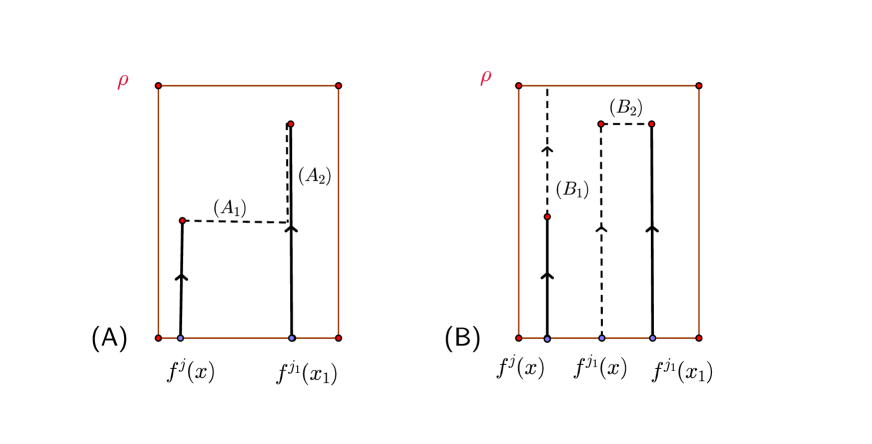
  Figure 1. Schematic description of the (dotted) vertical and horizontal segments used to estimate the Bowen-Walters distance: (A) corresponds to case (i) above; (B) corresponds to cases (ii) and (iii) below.

• The second case to consider is the case $j=j(x,s_{1},t)=j_{1}(x,s_{1},t)+1$. Noticing that $f^{j}(x)$ and $f^{j_{1}}(x)$ are consecutive elements of the same orbit, we get

  $$d_{\rho} (X_{t}(x,s_{1}),X_{t}(x_{1},s_{1}))$$

  $$=d_{1}\Big{(}\big{(}f^{j}(x),\frac{s_{1}+t-\sum_{i=0}^{j-1}\rho(f^{i}(x))}{\rho(f^{j}(x))}\big{)}\,,\,\big{(}f^{j_{1}}(x_{1}),\frac{s_{1}+t-\sum_{i=0}^{j_{1}-1}\rho(f^{i}(x_{1}))}{\rho(f^{j_{1}}(x_{1}))}\big{)}\Big{)}$$

  $$\leq d_{1}\Big{(}\big{(}f^{j_{1}}(x_{1}),\frac{s_{1}+t-\sum_{i=0}^{j_{1}-1}\rho(f^{i}(x_{1}))}{\rho(f^{j_{1}}(x_{1}))}\big{)}\,,\,\big{(}f^{j_{1}}(x),\frac{s_{1}+t-\sum_{i=0}^{j_{1}-1}\rho(f^{j}(x_{1}))}{\rho(f^{j_{1}}(x_{1}))}\big{)}\Big{)} B_{2}$$ ()

  $$+d_{1}\Big{(}\big{(}f^{j_{1}}(x),\frac{s_{1}+t-\sum_{i=0}^{j_{1}-1}\rho(f^{j}(x_{1}))}{\rho(f^{j_{1}}(x_{1}))}\big{)}\,,\,\big{(}f^{j}(x),\frac{s_{1}+t-\sum_{i=0}^{j-1}\rho(f^{i}(x))}{\rho(f^{j}(x))}\big{)}\Big{)} B_{1}$$ ()

  $$\leq\Big{(}1-\frac{s_{1}+t-\sum_{i=0}^{j_{1}-1}\rho(f^{i}(x_{1}))}{\rho(f^{j_{1}}(x_{1}))}\Big{)}\;d(f^{j_{1}}(x_{1}),f^{j_{1}}(x))$$

  $$+\;\frac{s_{1}+t-\sum_{i=0}^{j_{1}-1}\rho(f^{i}(x_{1}))}{\rho(f^{j_{1}}(x_{1}))}\;d(f^{j_{1}+1}(x_{1}),f^{j_{1}+1}(x))+(**)$$

  where $(**):=\Big{|}\big{(}1-\frac{s_{1}+t-\sum_{i=0}^{j_{1}-1}\rho(f^{i}(x_{1}))}{\rho(f^{j_{1}}(x_{1}))}\big{)}+\frac{s_{1}+t-\sum_{i=0}^{j-1}\rho(f^{i}(x))}{\rho(f^{j}(x))}\Big{|}$ (see Figure 1 above). Since $x$ was chosen so that its orbit to approximates the orbit of $x_{1}$ during the fist $n_{1}+1$ iterates then the sum of the first two terms is smaller than $\xi$. Since the two terms involved in the absolute value are positive and $j=j(x,s_{1},t)=j_{1}(x,s_{1},t)+1$ it follows from relations (14) that

  $$(**)=\frac{-s_{1}-t+\sum_{i=0}^{j_{1}}\rho(f^{i}(x_{1}))}{\rho(f^{j_{1}}(x_{1}))}+\frac{s_{1}+t-\sum_{i=0}^{j-1}\rho(f^{i}(x))}{\rho(f^{j}(x))}\leq\frac{C_{\xi}}{\inf\rho}+\frac{C_{\xi}}{\inf\rho}.$$

  Hence, we obtain that $d_{\rho}(X_{t}(x,s_{1}),X_{t}(x_{1},s_{1}))<\varepsilon$.

• If $j=j(x,s_{1},t)=j_{1}(x,s_{1},t)-1$ the computations are completely analogous to (ii) interchanging the roles of $x_{1}$ and $x$.

After the choice of the point $(x,s)$, partially determined by the gluing orbit property for $f$ and also by taking $s=s_{1}$, we claim that one can prove that the second assertion in the Claim is also satisfied. For each of the previous situations (i)-(iii) above (at time $t_{1}$) we will subdivide the proof in three additional cases, corresponding to the relative position of the lap number of $x$ and $x_{2}$. This will be made precise in the remaining of this section.

First assume case (i) above holds at time $t_{1}$, that is $j_{1}:=j(x,s_{1},t_{1})=j_{1}(x_{1},s_{1},t_{1})$ (c.f. Figure 2 below). In other words

$$X_{t_{1}}({x},s)=\Big{(}f^{j_{1}}(x),s_{1}+t_{1}-\sum_{i=0}^{j_{1}-1}\rho(f^{i}(x))\Big{)}\;\text{and}\;X_{t_{1}}(x_{1},s_{1})=\Big{(}f^{j_{1}}(x),s_{1}+t_{1}-\sum_{i=0}^{j_{1}-1}\rho(f^{i}(x))\Big{)}$$

where

$$\sum_{i=0}^{j_{1}-1}\rho(f^{i}(x))\leq s_{1}+t_{1}<\sum_{i=0}^{j_{1}}\rho(f^{i}(x))\quad\text{and}\quad\sum_{i=0}^{j_{1}-1}\rho(f^{i}(x_{1}))\leq s_{1}+t_{1}<\sum_{i=0}^{j_{1}}\rho(f^{i}(x_{1})).$$

Figure 2. The dotted line represents the piece of the trajectory of $x$ shadowing the piece of trajectory $X_{t}(f^{j_{1}}(x_{1}),0)$ for $t\in[0,s_{1}+t_{1}-\sum_{i=0}^{j_{1}-1}\rho(f^{i}(x))]$ and, after some time $p_{1}$, shadows the piece of trajectory $X_{t}(x_{2},s_{2})$ for a time $t\in[0,t_{2}]$.

In this case take

$$p_{1}=\begin{cases}\begin{array}[]{ll}s_{2}+\sum_{i=0}^{\tilde{p}_{1}-1}\rho(f^{j_{1}+i}(x))-[s_{1}+t_{1}-\sum_{i=0}^{j_{1}-1}\rho(f^{i}(x))],&\text{ if }s_{2}\leq\rho(f^{\tilde{p}_{1}+j_{1}}(x))\\ (s_{2}-C_{\xi})+\sum_{i=0}^{\tilde{p}_{1}-1}\rho(f^{j_{1}+i}(x))-[s_{1}+t_{1}-\sum_{i=0}^{j_{1}-1}\rho(f^{i}(x))],&\text{ otherwise. }\end{array}\end{cases}$$

In both cases above it is clear that $|p_{1}|\leq(\tilde{p}_{1}+2)\sup\rho\leq(N(\xi)+2)\sup\rho=T(\varepsilon)$. Now one can estimate $d_{\rho}(X_{t+p_{1}+t_{1}}(x,s_{1}),X_{t}(x_{2},s_{2}))$ according to the relative position of lap numbers.

If $s_{2}\leq\rho(f^{\tilde{p}_{1}+j_{1}}(x))$ then $X_{p_{1}+t_{1}}(x,s)=(f^{j_{1}+\tilde{p}_{1}}(x),s_{2})$. For any $t\in[0,t_{2}]$ set by, some abuse of notation, $j=j(f^{j_{1}+\tilde{p}_{1}}(x),s_{2},t)\in\mathbb{N}_{0}$ and $j_{2}=j_{2}(x_{2},s_{2},t)\in\mathbb{N}_{0}$ which are uniquely determined by

$$\sum_{i=0}^{j-1}\rho(f^{i+j_{1}+\tilde{p}_{1}}(x))\leq s_{2}+t<\sum_{i=0}^{j}\rho(f^{i+j_{1}+\tilde{p}_{1}}(x))\quad\text{and}\quad\sum_{i=0}^{j_{2}-1}\rho(f^{i}(x_{2}))\leq s_{2}+t<\sum_{i=0}^{j_{2}}\rho(f^{i}(x_{2})).$$ (15)

These lap numbers satisfy $|j(f^{j_{1}+\tilde{p}_{1}}(x),s_{2},t)-j_{2}(x_{2},s_{2},t)|\leq 1$ for every $t\in[0,t_{2}]$. Subdividing the later in three cases, when $j=j_{2}$, $j=j_{2}+1$ and $j=j_{2}-1$, we can deduce similarly as before that $d_{\rho}\Big{(}X_{t+p_{1}+t_{1}}(x,s_{1}),X_{t}(x_{2},s_{2})\Big{)}<\varepsilon$ for every $t\in[0,t_{2}]$.

If $s_{2}>\rho(f^{\tilde{p}_{1}+j_{1}}(x))$ then $X_{p_{1}+t_{1}}(x,s)=(f^{j_{1}+\tilde{p}_{1}}(x),s_{2}-C_{\xi})$. For any $t\in[0,t_{2}]$ set $j=j(f^{j_{1}+\tilde{p}_{1}}(x),s_{2}-C_{\xi},t)\in\mathbb{N}_{0}$ uniquely determined by

$$\sum_{i=0}^{j-1}\rho(f^{i+j_{1}+\tilde{p}_{1}}(x))\leq(s_{2}-C_{\xi})+t<\sum_{i=0}^{j}\rho(f^{i+j_{1}+\tilde{p}_{1}}(x))$$ (16)

and $j_{2}=j_{2}(x_{2},s_{2},t)\in\mathbb{N}_{0}$ determined by  (15). In the case that $j=j_{2}$,

$$d_{\rho} (X_{t+p_{1}+t_{1}}(x,s),X_{t}(x_{2},s_{2}))$$

$$=d_{1}\big{(}\big{(}f^{j+j_{1}+\tilde{p}_{1}}(x),\frac{s_{2}-C_{\xi}+t-\sum_{i=0}^{j-1}\rho(f^{i+j_{1}+\tilde{p}_{1}}(x))}{\rho(f^{j+j_{1}+\tilde{p}_{1}}(x))}\big{)},\big{(}f^{j_{2}}(x_{2}),\frac{s_{2}+t-\sum_{i=0}^{j_{2}-1}\rho(f^{i}(x_{2}))}{\rho(f^{j_{2}}(x_{2}))}\big{)}\big{)}$$

$$\leq d_{1}\big{(}\big{(}f^{j+j_{1}+\tilde{p}_{1}}(x),\frac{s_{2}-C_{\xi}+t-\sum_{i=0}^{j-1}\rho(f^{i+j_{1}+\tilde{p}_{1}}(x))}{\rho(f^{j+j_{1}+\tilde{p}_{1}}(x))}\big{)},\big{(}f^{j_{2}}(x_{2}),\frac{s_{2}-C_{\xi}+t-\sum_{i=0}^{j-1}\rho(f^{i+j_{1}+\tilde{p}_{1}}(x))}{\rho(f^{j+j_{1}+\tilde{p}_{1}}(x))}\big{)}\big{)}$$

$$+d_{1}\Big{(}\big{(}f^{j_{2}}(x_{2}),\frac{s_{2}-C_{\xi}+t-\sum_{i=0}^{j-1}\rho(f^{i+j_{1}+\tilde{p}_{1}}(x))}{\rho(f^{j+j_{1}+\tilde{p}_{1}}(x))}\big{)},\big{(}f^{j_{2}}(x_{2}),\frac{s_{1}+t-\sum_{i=0}^{j_{2}-1}\rho(f^{i}(x_{2}))}{\rho(f^{j_{2}}(x_{2}))}\big{)}\Big{)}$$

and consequently,

$$d_{\rho}(X_{t+p_{1}+t_{1}}(x,s),X_{t}(x_{2},s_{2})) \leq(1-\frac{s_{2}-C_{\xi}+t-\sum_{i=0}^{j-1}\rho(f^{i+j_{1}+\tilde{p}_{1}}(x))}{\rho(f^{j+j_{1}+\tilde{p}_{1}}(x))})\;d(f^{j+j_{1}+\tilde{p}_{1}}(x),f^{j_{2}}(x_{2}))$$

$$+\frac{s_{2}-C_{\xi}+t-\sum_{i=0}^{j-1}\rho(f^{i+j_{1}+\tilde{p}_{1}}(x))}{\rho(f^{j+j_{1}+\tilde{p}_{1}}(x))}\;d(f^{j+1+j_{1}+\tilde{p}_{1}}(x),f^{j_{2}+1}(x_{2}))$$

$$+\Big{|}\frac{s_{2}-C_{\xi}+t-\sum_{i=0}^{j-1}\rho(f^{i+j_{1}+\tilde{p}_{1}}(x))}{\rho(f^{j+j_{1}+\tilde{p}_{1}}(x))}-\frac{s_{2}+t-\sum_{i=0}^{j_{2}-1}\rho(f^{i}(x_{2}))}{\rho(f^{j_{2}}(x_{2}))}\Big{|}.$$

Since $j=j_{2}$ and points in the same dynamical ball for $f$ remain up to distance $\xi$ along the prescribed piece of orbit, the sum of the first two terms in the right hand side above are smaller than $\xi$. We shall bound differently the third summand in the right hand side above, which we will denote by $(***)$. By triangular inequality,

$$(***) \leq\Big{|}\frac{s_{2}-C_{\xi}+t-\sum_{i=0}^{j-1}\rho(f^{i+j_{1}+\tilde{p}_{1}}(x))-s_{2}-t+\sum_{i=0}^{j_{2}-1}\rho(f^{i}(x_{2}))}{\rho(f^{j+j_{1}+\tilde{p}_{1}}(x))}\Big{|}$$

$$+\frac{\big{(}s_{2}+t-\sum_{i=0}^{j_{2}-1}\rho(f^{i}(x_{2}))\big{)}}{\rho(f^{j+j_{1}+\tilde{p}_{1}}(x))\cdot\rho(f^{j_{2}}(x_{2}))}|\rho(f^{j+j_{1}+\tilde{p}_{1}}(x))-\rho(f^{j_{2}}(x_{2}))|\leq\frac{2C_{\xi}}{\inf\rho}+\frac{C_{\xi}}{\inf\rho}.$$

The estimates in the case $j=j_{2}-1$ and $j=j_{2}+1$ are obtained similarly. In consequence $d_{\rho}\big{(}X_{t+p_{1}+t_{1}}(x,s),X_{t}(x_{2},s_{2})\big{)}<\varepsilon$ for every $t\in[0,t_{2}]$.

Now assume case (ii) above at time $t_{1}$, that is, $j(x,s,t_{1})=j_{1}+1$ with $j_{1}=j_{1}(x_{1},s_{1},t)$ (see Figure 3 below).

Figure 3. Schematic picture where the dotted line represents the piece of the trajectory of $x$ shadowing the piece of trajectory $X_{t}(f^{j_{1}+1}(x_{1}),0)$ for $t\in[0,s_{1}+t_{1}-\sum_{i=0}^{j_{1}}\rho(f^{i}(x))]$ and, after some time $p_{1}$, follows the piece of the trajectory $X_{t}(x_{2},s_{2})$ for $t\in[0,t_{2}]$.

If this is the case take

$$p_{1}=\begin{cases}\begin{array}[]{ll}s_{2}+\sum_{i=0}^{\tilde{p}_{1}-1}\rho(f^{j_{1}+1+i}(x))-[s_{1}+t_{1}-\sum_{i=0}^{j_{1}}\rho(f^{i}(x))],&\text{ if }s_{2}\leq\rho(f^{\tilde{p}_{1}+j_{1}+1}(x))\\ (s_{2}-C_{\xi})+\sum_{i=0}^{\tilde{p}_{1}-1}\rho(f^{j_{1}+1+i}(x))-[s_{1}+t_{1}-\sum_{i=0}^{j_{1}}\rho(f^{i}(x))],&\text{ otherwise. }\end{array}\end{cases}$$

As above, $|p_{1}|\leq T(\varepsilon)$ in both cases. If $s_{2}\leq\rho(f^{\tilde{p}_{1}+j_{1}+1}(x))$ then computations completely identical to case (ii) proving $d_{\rho}\big{(}X_{t+p_{1}+t_{1}}(x,s),X_{t}(x_{2},s_{2})\big{)}<\varepsilon$ for every $t\in[0,t_{2}]$. In the case that $s_{2}>\rho(f^{\tilde{p}_{1}+j_{1}+1}(x))$ it follows that

$$d_{\rho} \big{(}X_{t+p_{1}+t_{1}}(x,s),X_{t}(x_{2},s_{2})\big{)}$$

$$=d_{1}\big{(}\big{(}f^{j+j_{1}+\tilde{p}_{1}}(x),\frac{s_{2}-C_{\xi}+t-\sum_{i=0}^{j-1}\rho(f^{i+j_{1}+\tilde{p}_{1}}(x))}{\rho(f^{j+j_{1}+\tilde{p}_{1}}(x))}\big{)},\big{(}f^{j_{2}}(x_{2}),\frac{s_{2}+t-\sum_{i=0}^{j_{2}-1}\rho(f^{i}(x_{2}))}{\rho(f^{j_{2}}(x_{2}))}\big{)}\big{)}$$

$$\leq d_{1}\Big{(}\big{(}f^{j_{2}}(x_{2}),\frac{s_{2}+t-\sum_{i=0}^{j_{2}-1}\rho(f^{i}(x_{2}))}{\rho(f^{j_{2}}(x_{2}))}\big{)}\,,\,\big{(}f^{j_{2}+j_{1}+\tilde{p}_{1}}(x),\frac{s_{2}+t-\sum_{i=0}^{j_{2}-1}\rho(f^{j}(x_{2}))}{\rho(f^{j_{2}}(x_{2}))}\big{)}\Big{)}$$

$$+d_{1}\Big{(}\big{(}f^{j_{2}+j_{1}+\tilde{p}_{1}}(x),\frac{s_{2}+t-\sum_{i=0}^{j_{2}-1}\rho(f^{j}(x_{2}))}{\rho(f^{j_{2}}(x_{2}))}\big{)}\,,\,\big{(}f^{j+j_{1}+\tilde{p}_{1}}(x),\frac{s_{2}-C_{\xi}+t-\sum_{i=0}^{j-1}\rho(f^{i+j_{1}+\tilde{p}_{1}}(x))}{\rho(f^{j+j_{1}+\tilde{p}_{1}}(x))}\big{)}\Big{)}$$

$$\leq\Big{(}1-\frac{s_{2}+t-\sum_{i=0}^{j_{2}-1}\rho(f^{j}(x_{2}))}{\rho(f^{j_{2}}(x_{2}))}\Big{)}\;d(f^{j_{2}}(x_{2}),f^{j_{2}+j_{1}+\tilde{p}_{1}}(x))$$

$$+\;\frac{s_{2}+t-\sum_{i=0}^{j_{2}-1}\rho(f^{j}(x_{2}))}{\rho(f^{j_{2}}(x_{2}))}\;d(f^{j_{2}+1}(x_{2}),f^{j_{2}+j_{1}+\tilde{p}_{1}+1}(x))+(\star)$$

where $(\star):=\Big{|}\big{(}1-\frac{s_{2}+t-\sum_{i=0}^{j_{2}-1}\rho(f^{j}(x_{2}))}{\rho(f^{j_{2}}(x_{2}))}\big{)}+\frac{s_{2}-C_{\xi}+t-\sum_{i=0}^{j-1}\rho(f^{i+j_{1}+\tilde{p}_{1}}(x))}{\rho(f^{j+j_{1}+\tilde{p}_{1}}(x))}\Big{|}$. By choose of $x$ follows that the sum of the first two terms is smaller than $\xi$. Since the two terms involved in the absolute value are positive and $j=j(f^{j_{1}+\tilde{p}_{1}}(x),s_{2}-C_{\xi},t)=j_{2}(x_{2},s_{2},t)+1$ we have

$$(\star)=\Big{|}-\frac{s_{2}+t-\sum_{i=0}^{j_{2}}\rho(f^{j}(x_{2}))}{\rho(f^{j_{2}}(x_{2}))}+\frac{s_{2}-C_{\xi}+t-\sum_{i=0}^{j-1}\rho(f^{i+j_{1}+\tilde{p}_{1}}(x))}{\rho(f^{j+j_{1}+\tilde{p}_{1}}(x))}\Big{|}\leq\frac{2C_{\xi}}{\inf\rho}+\frac{C_{\xi}}{\inf\rho}.$$

Hence, we obtain that $d_{\rho}(X_{t}(x,s_{1}),X_{t}(x_{1},s_{1}))<\varepsilon$.

If Case (iii) holds, for which $j(x,s,t_{1})=j_{1}(x_{1},s_{1},t)-1$, again completely analogous to Case (ii) with a modification on the definition of $p_{1}$ which must be replaced by

$$p_{1}=\begin{cases}\begin{array}[]{ll}s_{2}+\sum_{i=0}^{\tilde{p}_{1}-1}\rho(f^{j_{1}-1+i}(x))-[s_{1}+t_{1}-\sum_{i=0}^{j_{1}-2}\rho(f^{i}(x))],&\text{ if }s_{2}\leq\rho(f^{\tilde{p}_{1}+j_{1}-1}(x))\\ (s_{2}-C_{\xi})+\sum_{i=0}^{\tilde{p}_{1}-1}\rho(f^{j_{1}-1+i}(x))-[s_{1}+t_{1}-\sum_{i=0}^{j_{1}-2}\rho(f^{i}(x))],&\text{ otherwise. }\end{array}\end{cases}$$

The remaining estimates for the finite time shadowing necessary for proving the gluing orbit property are identical to the ones we have obtained above and for that reason we shall omit the details. This completes the proof of the theorem.

7.3. Proof of Theorem G

Assume that $f:M\to M$ satisfies the gluing orbit property. Let $\mu$ be an $f$-invariant ergodic probability measure and that the roof function $\rho:M\to\mathbb{R}_{0}^{+}$ is integrable. Fix $\varepsilon>0$. Consider arbitrary points $(x_{1},s_{1}),(x_{2},s_{2}),\dots,(x_{k},s_{k})\in M_{r}$ in a $\bar{\mu}$-full measure set in such a way that $\lim_{\xi\to 0}C_{\xi}(x_{i})=0$ for every $1\leq i\leq k$ and consider arbitrary times $t_{1},\dots,t_{k}\geq 0$. Associated to $(x_{i},s_{i})$ and $t_{i}$ consider the dynamical balls $B(x_{i},n_{i},\varepsilon)\subset M$, where $n_{i}=n_{i}(x_{i},s_{i},t_{i})\geq 1$ is determined by equation (13). Let $\xi>0$ be such that $\xi+C_{\xi}(x_{i})<\varepsilon$ for every $1\leq i\leq k$ and let $N(\xi)\geq 1$ be given by the gluing orbit property for $f$. Thus, there exists $x\in M$ and $\tilde{p}_{i}\leq N(\xi)$, $1\leq i\leq k$, so that $d(f^{j}(x),f^{j}(x_{1}))\leq\xi$ for every $0\leq j\leq n_{1}+1$ and $d(f^{j+n_{1}+\tilde{p}_{1}+\dots+n_{i-1}+\tilde{p}_{i-1}}(x)\,,\,f^{j}(x_{i}))\leq\xi$ for every $2\leq i\leq k$ and $0\leq j\leq n_{i}+1$. The proof follows the same strategy as in Theorem F with due care by the fact $\rho$ is not necessarily bounded but $\rho\in L^{1}(\mu)$. Take

$$T((x_{i},s_{i}),t_{i},\xi):=\sum_{j=0}^{\tilde{p}_{i}+2}\rho(f^{j+n_{i}-1}(x_{i}))+C_{\xi}(x_{i})$$

(where $\xi>0$ depends on $\varepsilon$) and decompose the terms as the pieces of the orbits of $x_{i}$ and the terms corresponding to the specified time lags $\tilde{p}_{i}$ as follows:

$$\frac{1}{n_{i}+\tilde{p}_{i}}\sum_{j=0}^{n_{i}+\tilde{p}_{i}}\rho(f^{j}(x_{i}))=\frac{n_{i}}{n_{i}+\tilde{p}_{i}}\;\frac{1}{n_{i}}\;\sum_{j=0}^{n_{i}-2}\rho(f^{j}(x_{i}))+\frac{n_{i}}{n_{i}+\tilde{p}_{i}}\;\frac{1}{n_{i}}\;\sum_{j=n_{i}-1}^{n_{i}+\tilde{p}_{i}+1}\rho(f^{j}(x_{i}))$$

Since the roof function $\rho$ is almost everywhere finite then $n_{i}=n_{i}((x_{i},s_{i}),t_{i})\to\infty$ as $t\to\infty$ and by Birkhoff’s ergodic theorem it follows that for $\overline{\mu}$-almost every $(x_{i},s_{i})$ the limit in second term in the right hand side is zero. Together with  (4), this proves that $\lim_{\xi\to 0}\lim_{t_{i}\to\infty}\frac{1}{n_{i}}\;T((x_{i},s_{i}),t_{i},\xi)=0$.

Let $x\in M$ be given by the gluing orbit property as above and let $s=s_{1}$. We claim that $d_{\rho}(X_{t}({x},s),X_{t}(x_{1},s_{1}))<\varepsilon$ for every $t\in[0,t_{i}]$ and there exists $0\leq p_{i}\leq T(\varepsilon)$ so that $d_{\rho}(X_{t+t_{1}+p_{1}}({x},s_{1}),X_{t}(x_{2},s_{2}))<\varepsilon$ for every $t\in[0,t_{i+1}]$.

Since the proof of the shadowing process is completely analogous to the proof of the Claim in Subsection 7.2 we will focus on the main difference which consists of expliciting the choice of the gluing times $p_{i}>0$. and keep the notation of that subsection. Thus we are reduced to prove the existence of $0\leq p_{i}\leq T((x_{i},s_{i}),t_{i},\xi)$ for which $d_{\rho}(X_{p_{i}}(X_{t_{i}}({x},s_{i})),(x_{i+1},s_{i+1}))<\varepsilon$. As in the proof of the previous theorem, we subdivide the argument for each choice of the gluing time in three cases.

If $j=j_{1}$ take

$$p_{1}=\begin{cases}\begin{array}[]{ll}s_{2}+\sum_{i=0}^{\tilde{p}_{1}-1}\rho(f^{i+j_{1}}(x))-[s_{1}+t_{1}-\sum_{i=0}^{j_{1}-1}\rho(f^{i}(x))],&\text{ if }s_{2}\leq\rho(f^{\tilde{p}_{1}+j_{1}}(x))\\ s_{2}-C_{\xi}+\sum_{i=0}^{\tilde{p}_{1}-1}\rho(f^{i+j_{1}}(x))+[\sum_{i=0}^{j_{1}-1}\rho(f^{i}(x))-(s_{1}+t_{1})]&\text{ otherwise. }\end{array}\end{cases}$$

If $j=j_{1}-1$ take

$$p_{1}=\begin{cases}\begin{array}[]{ll}s_{2}+\sum_{i=0}^{\tilde{p}_{1}-1}\rho(f^{i+j_{1}+1}(x))-[s_{1}+t_{1}-\sum_{i=0}^{j_{1}}\rho(f^{i}(x))],&\text{ if }s_{2}\leq\rho(f^{\tilde{p}_{1}+j_{1}+1}(x))\\ s_{2}-C_{\xi}+\sum_{i=0}^{\tilde{p}_{1}-1}\rho(f^{i+j_{1}+1}(x))+[\sum_{i=0}^{j_{1}}\rho(f^{i}(x))-(s_{1}+t_{1})]&\text{ otherwise. }\end{array}\end{cases}$$

If $j=j_{1}+1$ then take

$$p_{1}=\begin{cases}\begin{array}[]{ll}s_{2}+\sum_{i=0}^{\tilde{p}_{1}-1}\rho(f^{i+j_{1}-1}(x))-[s_{1}+t_{1}-\sum_{i=0}^{j_{1}-2}\rho(f^{i}(x))],&\text{ if }s_{2}\leq\rho(f^{\tilde{p}_{1}+j_{1}-1}(x))\\ s_{2}-C_{\xi}+\sum_{i=0}^{\tilde{p}_{1}-1}\rho(f^{i+j_{1}-1}(x))+[\sum_{i=0}^{j_{1}-2}\rho(f^{i}(x))-(s_{1}+t_{1})]&\text{ otherwise. }\end{array}\end{cases}$$

In all cases,

$$0\leq p_{1} \leq\sum_{j=0}^{\tilde{p}_{1}+2}\rho(f^{j+n_{1}-1}(x_{1}))\leq\sum_{j=0}^{\tilde{p}_{1}+2}\rho(f^{j+n_{1}-1}(x_{1}))+C_{\xi}=T((x_{1},s_{1}),t_{1},\xi).$$

This proves our claim and completes the proof of the theorem.

7.4. Proof of Theorem H

Let $f:M\to M$ satisfy the non-uniform specification property with respect to the ergodic and hyperbolic measure $\mu$ (c.f. [33, 50]) and assume the roof function $\rho:M\to\mathbb{R}_{0}^{+}$ is $\mu$-integrable and satisfies the bounded distortion condition (4).

By the non-uniform specification property for $(f,\mu)$, for $\mu$-almost every $x$, every $\xi>0$ and $n\geq 1$ there exists $p(x,n,\xi)\geq 1$ satisfying $\lim_{\xi\to 0}\limsup_{n\to\infty}p(x,n,\xi)/n=0$ and such that the following property holds: for every $k\geq 1$, $\mu^{k}$-almost every $(x_{1},\dots,x_{k})\in M^{k}$, every $n_{1},\dots,n_{k}\geq 1$ and $p_{i}\geq p(x_{i},n_{i},\xi)$ there exists $x\in M$ such that

$$\begin{array}[]{cc}d(f^{j}(x),f^{j}(x_{1}))\leq\xi\quad\text{and}\quad d(f^{j+n_{1}+p_{1}+\dots+n_{i-1}+p_{i-1}}(x)\;,\;f^{j}(x_{i}))\leq\xi\end{array}$$

for every $2\leq i\leq k$ and $0\leq j\leq n_{i}$.

We proceed to prove that the semiflow satisfies the non-uniform gluing orbit property. Fix $\varepsilon>0$. Consider arbitrary points $(x_{1},s_{1}),(x_{2},s_{2}),\dots,(x_{k},s_{k})\in M_{r}$ in a full $\overline{\mu}^{k}$-measure set and times $t_{1},\dots,t_{k}\geq 0$, in such a way that $\lim_{\xi\to 0C_{\xi}(x_{i})=0}$ for every $i$. Let $\xi>0$ be such that $\xi+C_{\xi}(x_{i})<\varepsilon$ for every $1\leq i\leq k$.

Associated to $(x_{i},s_{i})$ and $t_{i}$ consider the dynamical balls $B(x_{i},n_{i},\xi)\subset M$, where each lap number $n_{i}=n_{i}(x_{i},s_{i},t_{i})\geq 1$ is determined by equation (13). Let us define

$$T((x_{i},s_{i}),t_{i},\xi)=\sum_{j=0}^{p(x_{i},n_{i},\xi)+1}\rho(f^{j+n_{i}-1}(x_{i}))+C_{\xi}(x_{i}).$$

We claim that $T((x_{i},s_{i}),t_{i},\xi)$ has sublinear growth in $t_{i}$. Similarly to before one can write

$$\frac{1}{n_{i}+p(x_{i},n_{i},\varepsilon)+2}\sum_{j=0}^{n_{i}+p(x_{i},n_{i},\varepsilon)}\rho(f^{j}(x_{i})) =\frac{n_{i}-2}{n_{i}+p(x_{i},n_{i},\varepsilon)+2}\;\frac{1}{n_{i}-2}\;\sum_{j=0}^{n_{i}-2}\rho(f^{j}(x_{i}))$$ (17)

$$+\frac{1}{n_{i}+p(x_{i},n_{i},\varepsilon)+2}\;\sum_{j=0}^{p(x_{i},n_{i},\xi)+1}\rho(f^{j+n_{i}-1}(x_{i})).$$ (18)

Since the roof function $\rho$ is bounded away from zero then $n_{i}=n_{i}((x_{i},s_{i}),t_{i})\to\infty$ as $t_{i}\to\infty$ and

$$\lim_{\varepsilon\to 0}\lim_{t_{i}\to\infty}\frac{n_{i}}{n_{i}+p(x_{i},n_{i},\varepsilon)}=\lim_{\varepsilon\to 0}\lim_{t_{i}\to\infty}\frac{1}{1+\frac{p(x_{i},n_{i},\varepsilon)}{n_{i}}}=1.$$

Hence, by Birkhoff’s ergodic theorem the term (18) tends to zero as $t_{i}\to\infty$ for $\mu$-almost every $x_{i}$. Using $\lim_{\xi\to 0}C_{\xi}(x_{i})=0$ together with the previous equality, it follows that $\lim_{t_{i}\to\infty}\frac{1}{n_{i}}\;T((x_{i},s_{i}),t_{i},\varepsilon))=0$. We observe also that $\inf\rho\,n_{i}\leq\sum_{j=0}^{n_{i}}\rho(f^{j}(x))\leq s_{i}+t_{i}$ we deduce that $n_{i}\leq C\frac{t_{i}}{\inf\rho}$ and consequently $\lim_{\xi\to 0}\lim_{t_{i}\to\infty}\frac{1}{t_{i}}\;T((x_{i},s_{i}),t_{i},\xi))=0.$ Since the remaining of the proof follows the same lines of Theorem G we shall omit the details.

Appendix: On the tempered variation condition

In this Appendix we relate the tempered variation condition for observables on suspension semiflows with the corresponding condition for reduced observables on the base dynamics.

Proposition 7.1.

Let $(X_{t})_{t\geq 0}$ be a suspension semiflow over a dynamical system $f:M\to M$ with a roof function $\rho$ that is bounded away from zero and infinity and has tempered variation. If the observable $\psi:M_{\rho}\to\mathbb{R}$ is bounded and the reduced observable $\overline{\psi}:M\to\mathbb{R}$ has tempered variation then $\psi$ has tempered variation.

Proof.

Given $t,\delta>0$ and points $(x,t_{1})\in M_{\rho}$ and $(y,t_{2})\in B((x,t_{1}),t,\delta)$, using that $\inf\rho>0$, there exists $n\in\mathbb{N}_{0}$ such that either (i) $S_{n}\rho(x)\leq t$ and $S_{n}\rho(y)\leq t<S_{n+1}\rho(y)$ or (ii) $S_{n}\rho(y)\leq t$ and $S_{n}\rho(x)\leq t<S_{n+1}\rho(x)$. Assume that (i) holds since the other case is completely analogous. Then

$$\Big{|}\int_{0}^{t}\psi(X_{s}(x,t_{1}))-\psi(X_{s}(y,t_{2}))ds\Big{|} \leq\Big{|}\int_{0}^{S_{n}\rho(x)}\psi(X_{s}(x)ds-\int_{0}^{S_{n}\rho(y)}\psi(X_{s}(y)ds\,\Big{|}$$

$$+\Big{|}\int_{S_{n}\rho(x)}^{t}\psi(X_{s}(x)ds-\int_{S_{n}\rho(y)}^{t}\psi(X_{s}(y)ds\Big{|}$$

$$+\Big{|}\int_{0}^{t_{1}}\psi(X_{s}(x)ds-\int_{0}^{t_{2}}\psi(X_{s}(y)ds\,\Big{|}$$

$$\leq|S_{n}\overline{\psi}(x)-S_{n}\overline{\psi}(y)|+\Big{|}\int_{S_{n}\rho(x)}^{S_{n}\rho(y)}\psi(X_{s}(x))ds\Big{|}$$

$$+\Big{|}\int_{S_{n}\rho(y)}^{t}\psi(X_{s}(x))-\psi(X_{s}(y))ds\Big{|}+(t_{1}+t_{2})\sup|\psi|.$$

where we used $\bar{\psi}(x)=\int_{0}^{\rho(x)}\psi(X_{s}(x))\,ds$. Furthermore, we note that $y\in B_{f}(x,n,\delta)$ and that $\frac{t}{\inf\rho}\leq n\leq\frac{t}{\sup\rho}$ and, consequently, $n=n(t)\to\infty$ as $t\to\infty$. This yields that

$$\Big{|}\frac{1}{t}\int_{0}^{t}\psi(X_{s}(x))-\psi(X_{s}(y))ds\Big{|} \leq\frac{\sup|\psi|}{\inf\rho}\Big{[}\frac{1}{n}|S_{n}\overline{\psi}(x)-S_{n}\overline{\psi}(y)|+\frac{1}{n}|S_{n}\rho(x)-S_{n}\rho(y)|\Big{]}$$

$$+\frac{3}{n}\frac{\sup\rho\,\sup|\psi|}{\inf\rho}$$

tends to zero as $t\to\infty$. This proves that $\psi$ has tempered variation. ∎

Proposition 7.2.

Let $M$ be a compact metric space, $(X_{t})_{t}$ be a suspension semiflow over a bi-Lipschitz homeomorphism $f:M\to M$ with a Hölder continuous roof function $\rho$ and let $\mu$ be an $f$-invariant probability measure. Suppose that for every Hölder continuous observable $g$ there exists a constant $D>0$ such that

$$C_{\varepsilon}(g):=\sup_{n\in\mathbb{N}}\sup_{y\in B(x,n,\varepsilon)}\Big{|}\sum_{i=0}^{n-1}g(f^{i}(x))-\sum_{i=0}^{n-1}g(f^{i}(y))\Big{|}\leq D\varepsilon,$$

for every $\varepsilon>0$, and that $\phi:M\rightarrow{\mathbb{R}}$ is a potential bounded. Then

• If $\mu$ is a weak Gibbs measure for $f$ with respect to $\overline{\phi}$ then $(\mu\times\mbox{Leb})/\int\rho d\mu$ is weak Gibbs measure for $(X_{t})_{t\in\mathbb{R}}$ with respect to $\phi$.

• If $\mu$ is an $f$-invariant Gibbs measure for $f$ with respect to $\overline{\phi}$ then $(\mu\times\mbox{Leb})/\int\rho d\mu$ is a Gibbs measure for $(X_{t})_{t\in\mathbb{R}}$ with respect to $\phi$.

Proof.

Under the assumptions of the proposition, is proven in [7, Proposition 19] that there exists $\kappa>0$ so that for every $x\in M$, $0<s<\rho(x)$ and $m\in\mathbb{N}$ it holds that

$$B_{M_{\rho}}\big{(}(x,s),S_{m}\rho(x),\frac{1}{\kappa}\varepsilon\big{)}\subset B_{M}(x,m,\varepsilon)\times(s-\varepsilon,s+\varepsilon)\subset B_{M_{\rho}}\big{(}(x,s),S_{m}\rho(x),\kappa\varepsilon\big{)}$$

for every sufficiently small $\varepsilon$. In general, for $t>0$ there exists $m\in\mathbb{N}$, depending on $x$, so that $S_{m}\rho(x)\leq t+s<S_{m+1}\rho(x)$ and so

$$B_{M_{\rho}}\big{(}(x,s),S_{m+1}\rho(x),\varepsilon\big{)}\subset B_{M_{\rho}}\big{(}(x,s),t,\varepsilon\big{)}\subset B_{M_{\rho}}\big{(}(x,s),S_{m}\rho(x),\varepsilon\big{)}.$$

This implies that

$$\mu(B_{M}(x,m+1,\frac{\varepsilon}{\kappa})\times(s-\frac{\varepsilon}{\kappa},s+\frac{\varepsilon}{\kappa}))\leq\mu(B_{M_{\rho}}\big{(}(x,s),t,\varepsilon\big{)})\leq\mu(B_{M}(x,m,\kappa\varepsilon)\times(s-\kappa\varepsilon,s+\kappa\varepsilon))$$

and the desired result follows by simple integration. ∎

Acknowledgments

The authors are deeply grateful to V. Araújo and A. Arbieto for the incentive and suggestions that helped to improve the structure of the paper, and to C. Zhao for pointing out a mistake in a previous version of Theorem B. The second author was partially supported by a CNPq-Brazil posdoctoral fellowship at University of Porto and by CMUP (UID/MAT/00144/2013), which is funded by FCT (Portugal) with national (MEC) and European structural funds through the programs FEDER, under the partnership agreement PT2020.

References

• [1] D. V. Anosov. Geodesic flows on closed Riemannian manifolds of negative curvature Trudy Mat. Inst. Steklov. 90 (1967), 209.
• [2] D. V. Anosov and Y. Sinai. Some smoothly ergodic systems. Russian Mathematical Surveys 22, 1967, 103–167.
• [3] V. Araújo, M. J. Pacifico. Three-dimensional flows, volume 53 of Ergebnisse der Mathematik und ihrer Grenzgebiete. 3. Folge. A Series of Modern Surveys in Mathematics [Results in Mathematics and Related Areas. 3rd Series. A Series of Modern Surveys in Mathematics]. Springer, Heidelberg, 2010. With a foreword by Marcelo Viana.
• [4] V. Araújo. Large deviations bound for semiflows over a non-uniformly expanding base. Bull. Braz. Math. Soc. (N.S.) 38 (2007), no. 3, 335–376.
• [5] V. Araújo and A. Bufetov A large deviations bound for the Teichm ller flow on the moduli space of abelian differentials. Ergodic Theory Dynam. Systems 31 (2011), no. 4, 1043–1071.
• [6] A. Arbieto, L. Senos and T. Sodero, The specification property for flows from the robust and generic viewpoint, J. Differential Equations 253 (2012), 1893–1909.
• [7] L. Barreira and B. Saussol. Multifractal analysis of hyperbolic flows. Comm. Math. Phys. 214 (2000) 339–371.
• [8] M. Bessa, M. J. Torres and P. Varandas, Topologically transitiveness and shadowing is $C^{1}$-generic among geodesic flows with bounded curvature. Preprint 2015.
• [9] T. Bomfim and P. Varandas, Multifractal analysis for weak Gibbs measures: from large deviations to irregular sets. Ergod. Th. $\&$ Dynam. Sys. (to appear)
• [10] A.M. Blokh, Decomposition of dynamical systems on an interval, Russ. Math. Surv. 38 (1983), 133-134.
• [11] R. Bowen. Entropy for group endomorphisms and homogeneous spaces. Trans. Amer. Math. Soc., 153 (1971), 401–414.
• [12] R. Bowen, Periodic orbits for hyperbolic flows, Amer. J. Math. 94, (1972), 1–30.
• [13] R. Bowen. Equilibrium states and the ergodic theory of Anosov diffeomorphisms, volume 470 of Lect. Notes in Math. Springer Verlag, 1975.
• [14] R. Bowen, Some systems with unique equilibrium states Math. Syst. Theory 8 (1974), 193–202.
• [15] R. Bowen and D. Ruelle. The ergodic theory of Axiom A flows. Invent. Math., 29:181–202, 1975.
• [16] V. Climenhaga and D. Thompson Equilibrium states beyond specification and the Bowen property. Journal London Math Soc. 87 (2013), 401–427.
• [17] K. Burns, V. Climenhaga, T. Fisher and D. Thompson. Unique equilibrium states for geodesic flows in nonpositive curvature Preprint 2015.
• [18] M. Field, I. Melbourne, and A. Törok. Stability of mixing and rapid mixing for hyperbolic flows. Annals of Mathematics, 166:269–291, 2007.
• [19] S. Gan and L. Wen. Nonsingular star flows satisfy Axiom A and the no-cycle condition, Invent. Math. 164 (2006), 279–315.
• [20] S. Gan, L. Wen and S. Zhu. Indices of singularities of robustly transitive sets, Discrete Contin. Dyn. Syst. 21 (3) (2008) 945–957.
• [21] N. T. A. Haydn and D. Ruelle Equivalence of Gibbs and equilibrium states for homeomorphisms satisfying expansiveness and specification Comm. Math. Phys., 148, 1 (1992), 155–167.
• [22] H. Hu and L-S. Young. Nonexistence of SBR measures for some diffeomorphisms that are “Almost Anosov”. Ergog. Th. Dynam. Sys., 15:1 (1995) 67–76.
• [23] A. Katok. Lyapunov exponents, entropy and periodic orbits for diffeomorphisms. Inst. Hautes Etudes Sci. Publ. Math.,51:137 –173,1980.
• [24] Y. Kifer. Large deviations in dynamical systems and stochastic processes. Trans. Amer. Math. Soc., 321(2) (1990), 505–524.
• [25] Y. Kifer and S. Newhouse. A global volume lemma and applications. Israel J. Math. 74 (1991), no. 2–3, 209–223.
• [26] D. Kwietniak, M. Lacka, P. Oprocha. A panorama of specification-like properties and their consequences. Contemporary Mathematics (to appear).
• [27] C. Liverani. On contact Anosov flows. Ann. of Math. (2), 159(3):1275–1312, 2004.
• [28] R. D. Mauldin and M. Urbanski. Gibbs states on the symbolic space over an infinite alphabet. Israel J. Math. 125 (2001), 93–130.
• [29] I. Melbourne. Large and moderate deviations for slowly mixing dynamical systems. Proc. Amer. Math. Soc. 137 (2009), no. 5, 1735–1741.
• [30] I. Melbourne and M. Nicol. Large deviations for nonuniformly hyperbolic systems. Trans. Amer. Math. Soc., 360:6661–6676, 2008.
• [31] K. Moriyasu, K. Sakai, N. Sumi, Vector fields with topological stability, Trans. Amer. Math. Soc. 353 (8) (2001) 3391–3408.
• [32] V. Oseledets, A multiplicative ergodic theorem: Lyapunov characteristic numbers for dynamical systems, Trans. Moscow Math. Soc., 19, (1968), 197–231.
• [33] K. Oliveira and X.Tian. Non-uniform hyperbolicity and non-uniform specification. Trans. Amer. Math. Soc., 365 (2013), 4371–4392.
• [34] M. Pollicott. On the mixing of Axiom A attracting flows and a conjecture of Ruelle. Ergodic Theory Dynam. Systems 19 (1999), no. 2, 535–548.
• [35] C.-E. Pfister and W. Sullivan. Large Deviations Estimates for Dynamical Systems without the Specification Property Application to the Beta-Shifts. Nonlinearity, 18 (2005), 237–261.
• [36] C. Pugh, An improved closing lemma and a general density theorem, Amer. J. Math. 89 (1967) 1010–1021.
• [37] J. Rousseau, P. Varandas and Y. Zhao, Entropy formulas for dynamical systems with mistakes, Discrete and Continuous Dynamical Systems - A, 32:12,4391–4407 (2012).
• [38] D. Ruelle. A measure associated with Axiom A attractors. Amer. J. Math., 98:619–654, 1976.
• [39] D. Ruelle. Flots qui ne mélangent pas exponentiellement. C. R. Acad. Sci. Paris Sér. I Math., 296(4):191–193, 1983.
• [40] D. Ruelle Thermodynamic formalism for maps satisfying positive expansiveness and specification. Nonlinearity 5, 1223–1226(1992).
• [41] K. Sakai, N. Sumi and K. Yamamoto. Diffeomorphisms satisfying the specification property. Proc. Amer. Math. Soc., 138 (2009), 315–321.
• [42] Ya. Sinai, Markov partitions and C-diffeomorphisms. Func. Anal. and Appl., 2, (1968), 64–89.
• [43] K. Sigmund. On dynamical systems with the specification property. Trans. Amer. Math. Soc. 190 (1974), 285–299.
• [44] S. Smale. Differentiable dynamical systems. Bull. Amer. Math. Soc., 73:747–817, 1967.
• [45] N. Sumi, P. Varandas and K.Yamamoto Partial hyperbolicity and specification. Proc. Amer. Math. Soc. (to appear 2015).
• [46] N. Sumi, P. Varandas and K.Yamamoto Partial hyperbolicity and specification for flows. Preprint CMUP 2015-3.
• [47] W. Sun and X. Tian Diffeomorphisms with various $C^{1}$-stable properties. Acta Mathematica Scientia 2012, 32B(2):552–558.
• [48] H. Totoki. Time changes for flows. Memoirs of the Faculty of Science, Kyushu Univ. Ser. A, 20 (1), 1966, 27–55.
• [49] P. Varandas and M. Viana. Existence, uniqueness and stability of equilibrium states for non-uniformly expanding maps, Annales de l’Institut Henri Poincaré- Analyse Non-Linaire, 27:555–593, 2010.
• [50] P. Varandas. Non-uniform specification and large deviations for weak Gibbs measures. J. Statist. Phys., 146 (2012), 330–358.
• [51] S. Waddington. Large deviations asymptotics for Anosov flows. Ann. Inst. H. Poincar Sect. C 13(4) (1996), 445–484.
• [52] P. Walters, An introduction to ergodic theory, Springer-Verlag, New York, 1982.
• [53] L.-S. Young. Some large deviation results for dynamical systems. Trans. Amer. Math. Soc., 318(2) (1990), 525–543.