Statistical Physics of Neural Systems
with Non-additive Dendritic Coupling

Abstract

How neurons process their inputs crucially determines the dynamics of biological and artificial neural networks. In such neural and neural-like systems, synaptic input is typically considered to be merely transmitted linearly or sublinearly by the dendritic compartments. Yet, single-neuron experiments report pronounced supralinear dendritic summation of sufficiently synchronous and spatially close-by inputs. Here, we provide a statistical physics approach to study the impact of such non-additive dendritic processing on single neuron responses and the performance of associative memory tasks in artificial neural networks. First, we compute the effect of random input to a neuron incorporating nonlinear dendrites. This approach is independent of the details of the neuronal dynamics. Second, we use those results to study the impact of dendritic nonlinearities on the network dynamics in a paradigmatic model for associative memory, both numerically and analytically. We find that dendritic nonlinearities maintain network convergence and increase the robustness of memory performance against noise. Interestingly, an intermediate number of dendritic branches is optimal for memory functionality.

Keywords: statistical physics, neural networks, associative memory, nonlinear dendrites

PACS: 05.20.-y, 87.19.L-, 84.35.+i

I Introduction: Non-additive dendritic input processing in neural networks

Information processing in artificial and biological neural networks crucially depends on the processing of inputs in single neurons (e.g. Koch and Segev, (2000)). The dendrites, branched protrusions of a biological nerve cell or the input preprocessing of formal neurons constitute the main input sites. Traditionally, dendrites are modeled as passive, cable-like conductors which integrate incoming presynaptic signals linearly or sublinearly and propagate the change in voltage to the cell body or soma where it is subject to nonlinear transformations Stuart et al., (2007). Accordingly, the input preprocessing in formal neurons is usually assumed to be a linear or sublinear summation.

Single-neuron experiments, however, demonstrate the occurrence of strongly supralinear dendritic amplification. Biophysically, this is caused by action potentials generated in the dendrite of the neuron. Such dendritic spikes are mediated by voltage-dependent ion channels such as sodium, calcium, and NMDA channels Ariav et al., (2003); Gasparini et al., (2004); Polsky et al., (2004); Nevian et al., (2007); Larkum and Nevian, (2008). In particular, dendritic spikes may emerge if sufficiently synchronous inputs are received by the same branch of a dendrite. The many inputs to the dendrites can thus be processed non-additively, depending on their spatial and temporal distribution Poirazi et al., 2003a ; Polsky et al., (2004). This implies crucial deviations from the classical assumptions on linear dendritic input processing as modeled, e.g., by cable equations. It has been recently shown that dendritic spikes are present and prominent all over the brain (e.g. London and Häusser, (2005)).

A number of theoretical studies highlighted the importance of nonlinear, spiking dendrites already for the input processing in single neurons: Simulations of neuron models with detailed channel density and morphology showed dendritic spike generation in agreement with neurobiological experiments Ariav et al., (2003); Poirazi et al., 2003b ; Poirazi et al., 2003a ; Gasparini et al., (2004); Nevian et al., (2007). Further, firing rate models have been developed Mel, 1992a which reproduce the response properties of detailed models to diverse stimuli and behave like multi-layered feed-forward networks of simple rate neurons Poirazi et al., 2003b ; Poirazi et al., 2003a ; Polsky et al., (2004). Two and multi-layer feed-forward networks of binary, deterministic neurons have been studied using statistical physics methods Barkai et al., (1990); Hertz et al., (1991); Biehl et al., (2000). In particular, the so-called committee machine may be seen as a neuron model incorporating a layer of dendrites with step-like activation functions, i.e. without analogous signal transmission Engel et al., (1992); Urbanczik, (1997). Neurons in biological networks receive time dependent, noisy input at high rates which often makes a statistical description of the response properties of single neurons necessary. In Ref. Ujfalussy et al., (2009), the authors derived such a description for linear and quadratic dendritic summation together with some numerical results for a biologically plausible, sigmoidal dendritic nonlinearity. The propagation of dendritic spikes in branched dendrites with step-like activation functions has been studied in Ref. Gollo et al., (2012), providing the somatic input as a numerical solution to a high-dimensional system of nonlinear equations. To date there is no efficient statistical description for neurons with biologically plausible, sigmoidal dendritic nonlinearities. In biological systems, neurons form complex, recurrent networks. Thus, a description which allows to analytically study networks of neurons with multiple nonlinear dendrites is especially desirable.

Recent single neuron experiments investigated the role of active dendrites in detecting specific spatio-temporal input patterns Schiller and Schiller, (2001); Gasparini et al., (2004); Losonczy et al., (2008). Theoretical studies showed that nonlinear dendrites improve the ability of single neurons and ensembles of single neurons to discriminate and learn different input patterns Mel, 1992b ; Poirazi and Mel, (2001); Rhodes, (2008); Schiess et al., (2012). Besides trivially multiplying the single neuron abilities to detect input patterns, a network of neurons can store, retrieve and complete spatio-temporal patterns aided by its recurrent dynamics: It can function as an associative memory device Hopfield, (1982); Amit et al., 1985a ; Hertz et al., (1991). Yet, the impact of nonlinear dendrites on associative memory networks is unknown.

So far, only few studies considered the impact of non-additive dendrites on network dynamics. Selectivity and invariance of network responses to external stimuli and their intensity were analyzed in a firing rate model Morita et al., (2007); Morita, (2008). Refs. Lisman et al., (1998); Wang, (2001); Morita, (2008) proposed that NMDA-receptor dependent dendritic nonlinearities play a crucial role in working memory, i.e., in the formation of persistent activity in unstructured networks. Nonlinear, multiplicative dendritic processing arising from spatial summation of input across the dendritic arbor was similarly shown to enable spontaneous and persistent network activity Zhang et al., (2013). Dendritic spikes were suggested to work as coincidence detectors and provide a neuronal basis for temporal and spatial context in biological networks Katz et al., (2007); Stuart and Häusser, (2001). Refs. Long et al., (2010); Traub and Wong, (1982) studied networks of bursting neurons, where the bursts facilitate the emergence of patterns of coordinated neuronal activity and can be explained by dendritic spikes. Further, it was shown that nonlinear dendrites can enable robust propagation of synchronous spiking in random networks with biologically plausible substructures Jahnke et al., (2012) and in purely random networks Memmesheimer and Timme, (2012). Finally, dendritic spikes were related to so-called sharp-wave ripples in the hippocampus which are important for long-term memory consolidation Memmesheimer, (2010).

Networks of binary neurons with linear input summation have been intensively investigated in statistical physics (“Hopfield networks”, Hopfield, (1982); Amit et al., 1985a ; Hertz et al., (1991)) and extensions to different nonlinear and non-monotonic transfer functions exist (cf. e.g. Hopfield, (1984); Shiino, (1990); Morita, (1993); Inoue, (1996); Qiao et al., (2001)). All of these studies assumed point-neurons, neural networks of arborized neurons with non-additive coupling have not been studied in comparable setups. Hopfield networks are paradigmatic models for associative memory which may in particular contribute to solving two important conundrums in Neuroscience: how biological neural networks achieve a high memory capacity and how they can work so reliably under the experimentally found noisy conditions. The incorporation of non-additive dendrites into these models may therefore (1) shed light on the impact of these features on memory capacity and robustness and, at the same time, (2) allow to understand the underlying mechanisms due to their analytical tractability.

In the first part of this article, we describe the response properties of single neurons in presence of biologically plausible dendritic nonlinearities in a statistical framework. In the second part, we employ the results and study the effect of nonlinear dendrites on associative memory networks. We consider networks of the Hopfield type, as this standard model for associative memory lends itself to analytical treatment and allows to concisely work out the effects of nonlinear dendritic enhancement. We find that dendritic nonlinearities improve pattern retrieval by effectively reducing the thresholds of neurons and by increasing the robustness to noise. The improvement is strongest for intermediate numbers of dendritic branches. We quantify these effects and illustrate our analytical findings with numerical simulations.

II Results

II.1 Basic model for non-additive processing in dendrites

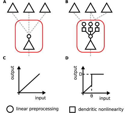
Figure 1: Arborized neuron with dendritic nonlinearities. Network architecture for a classical point-neuron model without dendrites (A) and an arborized neuron with $B=3$ dendrites (or dendritic branches) modeled as separate compartments (B). The red boxes mark the neuronal unit for each case. Circles represent linear summation of inputs (C), triangles and squares represent somatic and dendritic processing, respectively. In a point-neuron all inputs are summed up linearly and then processed nonlinearly. In a model with nonlinear dendrites there is an additional, preceding layer where inputs to each dendrite are summed up linearly and then subjected to a dendritic nonlinearity. This nonlinearity is modeled as a piecewise linear function with threshold $\theta$ and saturation strength $D$, incorporating the effect of dendritic spikes (D). The somatic transfer function is not constrained in the model.

Consider an extended topological structure of a neuron consisting of one point-like soma and $B$ independent dendritic compartments (Fig. 1). Each compartment receives its inputs from a number of presynaptic neurons and transfers its output to the soma. We assume that nonlinear dendritic integration takes place over a time window $\Delta t$. Our model can be applied to dendrites with fast or slow dendritic spikes, where $\Delta t$ assumes values of $2-3\,\mathrm{ms}$ (fast, sodium spikes Ariav et al., (2003); Gasparini et al., (2004)) or tens of $\mathrm{ms}$ (slow, e.g. NMDA spikes Schiller et al., (2000); Polsky et al., (2004)). The durations of the different dendritic spikes have timescales similar to their integration windows. The input arriving at a branch within $\Delta t$ is denoted by $u$. On each branch, we capture the non-additive input summation of the dendrites through a piecewise linear, sigmoidal transfer function

$$f\left(u\right) := \begin{cases}u&\mbox{ if }u<\theta\\ D&\mbox{ otherwise}.\end{cases}$$ (1)

If$u$ is smaller than a threshold $\theta$, i.e. $u<\theta$, the inputs superpose linearly. Biologically, this means that $u$ has not reached the threshold $\theta$ for dendritic spike generation and that it is conventionally transferred to the soma. If the threshold is exceeded, i.e. $u\geq\theta$, the inputs superpose non-additively and a fixed dendritic output strength $D$ is attained. This models the effect of a dendritic spike elicited by sufficiently strong input. The summation scheme as well as the compartmentalization are in agreement with experimental findings and modeling studies Ariav et al., (2003); Poirazi et al., 2003a ; Gasparini et al., (2004); Polsky et al., (2004); Morita et al., (2007); Memmesheimer, (2010). Our approaches may be directly extended to neurons with multiple stages of dendritic processing (cf. App. A3).

II.2 Capturing dendritic spikes by an effective somatic input strength

To quantify the impact of non-additive dendritic events on the neuronal input processing, the temporal and spatial distribution of synaptic input must be taken into account. We consider a neuron with $B$ dendritic branches $b\in\left\{1,\ldots,B\right\}$ and some time interval of the length of the dendritic integration window. $x_{b}$ denotes the number of synapses on branch $b$ that are active within this window. The numbers of active synapses are distributed according to $P\left(x_{1},\dots,x_{B}\right)$. Furthermore, we allow for distributed connection strengths by assigning the synapses weights $w$ which are independently and identically distributed according to $P\left(w\right)$. Averages with respect to $P\left(x_{1},\dots,x_{B}\right)$ and $P\left(w\right)$ can be interpreted as ensemble averages or temporal averages. The ensemble average is taken over a large number of neurons at a fixed time where each neuron has numbers $x_{b}$ of active inputs and weights $w$ which are samples of $P\left(x_{1},\dots,x_{B}\right)$ and $P\left(w\right)$, respectively. Under the additional assumption of a large number of synaptic contacts on each branch, the averages may also be understood as time averages which are taken at a fixed neuron over a suitably segmented long time interval in which the active inputs are changing. In this article, we follow the first interpretation of ensemble averages.

What is the effective input to the soma given that synaptic inputs are distributed across branches? We assume that each branch samples a volume in which synapses of axons from $S$ other (presynaptic) neurons can be synaptically contacted Abeles, (1991). A synapse is present and active with probability $p_{b}$ such that $P\left(x_{1},\dots,x_{B}\right)$ is a product of binomial distributions with means $\mathrm{E}\left[x_{b}\right]=Sp_{b}$ and variances $\mathrm{Var}\left[x_{b}\right]=Sp_{b}\left(1-p_{b}\right)$. Alternatively, the total number of active synaptic terminals across branches might be fixed to $S$ (e.g. due to homeostatic learning) which suggests a multinomial distribution for $P\left(x_{1},\dots,x_{B}\right)$. Then, the $x_{b}$ on different branches are not independent but negatively correlated with covariances $\mathrm{Cov}\left[x_{b},x_{c}\right]=-Sp_{b}p_{c}$ for $b,c\in\left\{1,\dots,B\right\}$ and $b\neq c$.

The input to branch $b$ is given by the linear sum

$$u_{b} = \sum_{i=1}^{x_{b}}w_{i}$$ (2)

and we are interested in the distribution $P\left(u_{1},\dots,u_{B}\right)$ of input across branches. According to Wald’s equation Wald, (1944), the Blackwell-Girshick equation Blackwell and Girshick, (1946) and the conditional covariance formula Sheldon, (2002), we have for $b\neq c$,

$$\mathrm{E}\left[u_{b}\right] = \mathrm{E}\left[x_{b}\right]\mathrm{E}\left[w\right],$$ (3)

$$\mathrm{Var}\left[u_{b}\right] = \mathrm{E}\left[x_{b}\right]\mathrm{Var}\left[w\right]+\mathrm{Var}\left[x_{b}\right]\mathrm{E}^{2}\left[w\right],$$ (4)

$$\mathrm{Cov}\left[u_{b},u_{c}\right] = \mathrm{E}\left[\mathrm{Cov}\left[u_{b},u_{c}\mid x_{b},x_{c}\right]\right]$$ (5)

$$+\mathrm{Cov}\left[\mathrm{E}\left[u_{b}\mid x_{b},x_{c}\right],\mathrm{E}\left[u_{c}\mid x_{b},x_{c}\right]\right]$$

$$= \mathrm{Cov}\left[x_{b},x_{c}\right]\mathrm{E}^{2}\left[w\right],$$

where $\mathrm{Cov}\left[u_{b},u_{c}\mid x_{b},x_{c}\right]=0$ and $\mathrm{E}\left[u_{b}\mid x_{b}\right]=x_{b}\mathrm{E}\left[w\right]$ due to the independence of the synaptic weights $w$. $P\left(u_{1},\dots,u_{B}\right)$ is in general a complicated distribution (App. A2). Since its first moments are known (Eqs. (3)-(5)) we approximate $P\left(u_{1},\dots,u_{B}\right)$ by a multivariate normal distribution, i.e. by the maximum entropy distribution for the given moments.

This enables us to derive an effective input to the soma that depends only on the number $B$ of branches, the probabilities $p_{b}$, $S$, and the moments $\mathrm{E}\left[w\right]$ and $\mathrm{Var}\left[w\right]$. For only linear branches, i.e. $u_{b}<\theta$ on all branches, the input to the soma is simply given by the linear sum $\sum_{b=1}^{B}u_{b}$. For $u_{b}\geq\theta$, the dendritic nonlinearity sets in and branch $b$ provides input of strength $D$ to the soma. Since somatic preprocessing is linear, the total input to the soma is

$$F =F\left(u_{1},\ldots,u_{B}\right)= \sum_{b=1}^{B}f\left(u_{b}\right).$$ (6)

The evaluation of the sum is numerically simple but denies analytical treatment. Yet, for Gaussian $P\left(u_{1},\dots,u_{B}\right)$, we may compute its mean (App. A1) via

$$\mathrm{E}\left[F\right] = \prod_{b=1}^{B}\int_{-\infty}^{\infty}\mathrm{d}u_{b}\left(\sum_{b=1}^{B}f\left(u_{b}\right)\right)P\left(u_{1},\dots,u_{B}\right)$$ (7)

$$= B\left(\int_{\theta}^{\infty}\mathrm{d}uDP\left(u\right)+\int_{-\infty}^{\theta}\mathrm{d}uuP\left(u\right)\right)$$

$$= BP_{\mathrm{NL}}D+B\left(1-P_{\mathrm{NL}}\right)E\left[u\right]-BC_{\mathrm{NL}},$$

where we exploited that the marginal distribution $P\left(u\right)$ of the multivariate normal distribution $P\left(u_{1},\dots,u_{B}\right)$ is a normal distribution again and defined

$$P_{\mathrm{NL}} := \frac{1}{2}\mathrm{erfc}\left(\frac{\theta-\mathrm{E}\left[u\right]}{\sqrt{2\mathrm{Var}\left[u\right]}}\right),$$ (8)

$$C_{\mathrm{NL}} := \sqrt{\frac{\mathrm{Var}\left[u\right]}{2\pi}}\exp\left(-\frac{\left(\theta-\mathrm{E}\left[u\right]\right)^{2}}{2\mathrm{Var}\left[u\right]}\right).$$ (9)

In the second line of Eq. (7) we assumed $p_{b}=p_{0}$, where $p_{0}$ is a constant probability independent of $b$. Throughout the rest of the article we follow this choice for simplicity, although many results are independent of $p_{b}$ or may be easily generalized to arbitrary $p_{b}$. Eq. (7) may be interpreted as follows: The first part describes the expected number $BP_{\mathrm{NL}}$ of dendritic spikes of strength $D$, while the second part captures $B\left(1-P_{\mathrm{NL}}\right)$ linear events, and the last part $BC_{\mathrm{NL}}$ corrects the overestimate of the contribution of the linear branches by $\mathrm{E}\left[u\right]$. To obtain the variance $\mathrm{Var}\left[F\right]=\mathrm{E}\left[F^{2}\right]-\mathrm{E}^{2}\left[F\right]$, we analogously derive the second moment (App. A1)

$$\mathrm{E}\left[F^{2}\right] = \prod_{b=1}^{B}\int_{-\infty}^{\infty}\mathrm{d}u_{b}\left(\sum_{b=1}^{B}f\left(u_{b}\right)\right)^{2}P\left(u_{1},\dots,u_{B}\right)$$ (10)

$$= B\int_{-\infty}^{\infty}\mathrm{d}uf^{2}\left(u\right)P\left(u\right)$$

$$+\left(B^{2}-B\right)\int_{-\infty}^{\infty}\int_{-\infty}^{\infty}\mathrm{d}u\mathrm{d}vf\left(u\right)f\left(v\right)P\left(u,v\right).$$

$P\left(u,v\right)$ is the marginal distribution of $P\left(u_{1},\dots,u_{B}\right)$ in two variables. For binomially distributed synapses, $P\left(u,v\right)=P\left(u\right)P\left(v\right)$ factors into two independent normal distributions which yields

$$\mathrm{E}\left[F^{2}\right] = BP_{\mathrm{NL}}D^{2}+B\left(1-P_{\mathrm{NL}}\right)\left(\mathrm{E}^{2}\left[u\right]+\mathrm{Var}\left[u\right]\right)$$ (11)

$$-BC_{\mathrm{NL}}\left(\mathrm{E}\left[u\right]+\theta\right)+\left(B^{2}-B\right)B^{-2}\mathrm{E}^{2}\left[F\right].$$

For multinomially distributed synapses, the double integral in Eq. (10) needs to be evaluated numerically (see App. A1 and Fig. 2).

The mean $\mathrm{E}\left[F\right]$ and its variance $\mathrm{Var}\left[F\right]$ (as well as the expected number $\mathrm{E}\left[k\right]$ of nonlinear branches and its variance $\mathrm{Var}\left[k\right]$, see below) may also be computed without the Gaussian approximation employing the exact expression for $P\left(u_{1},\dots,u_{B}\right)$ (App. A2).

We note that our approximation can be employed to compute the input statistics to neurons with several layers of non-additive dendritic branches by iteratively applying the formulas for $\mathrm{E}\left[F\right]$ and $\mathrm{Var}\left[F\right]$ (Eqs. (7)-(10)) to each branching point and using the result as a new input to the next layer (cf. App. A3 for a derivation).

II.3 Features of the somatic input

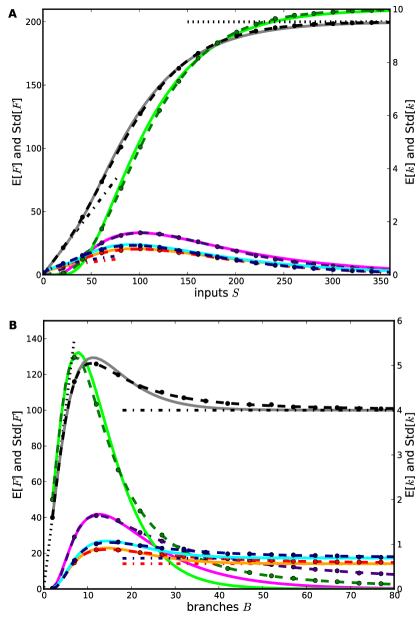
Figure 2: Mean and standard deviation of the somatic input $F$, optimal number of branches. Results for fixed $B=10$ and varying $S$ (A) and vice versa, with $S=100$ (B). Remaining parameters are $\theta=10$, $D=20$, $p_{0}=B^{-1}$ and $P\left(w\right)$ is Gaussian with mean $\mathrm{E}\left[w\right]=1$ and variance $\mathrm{Var}\left[w\right]=2$. The effective somatic input $\mathrm{E}\left[F\right]$, the average number of nonlinear branches $\mathrm{E}\left[k\right]$ and their standard deviations $\mathrm{Std}\left[F\right]=\sqrt{\mathrm{Var}\left[F\right]}$ and $\mathrm{Std}\left[k\right]=\sqrt{\mathrm{Var}\left[k\right]}$ are derived numerically using $2000$ realizations of binomially and multinomially distributed synapses (circles). They agree well with the Gaussian approximation (solid lines) and the exact analytical solution (dashed lines). $\mathrm{E}\left[F\right]$ are shown in black (exact solution, dashed) and gray (Gaussian approximation, solid), $\mathrm{Std}\left[F\right]$ are colored blue and cyan for binomially distributed synapses and red and orange for multinomially distributed synapses. Averages $\mathrm{E}\left[k\right]$ are colored green and lime and their variances $\mathrm{Std}\left[k\right]$ for the binomial scenario are shown in purple and pink. Dash-dotted and dotted lines represent the linear and saturated limits, respectively. See main text for a detailed discussion.

We compare the input $F$ to the soma from numerical simulations (Eq. (6) and Fig. 2, circles), from the Gaussian approximation (Eqs. (7) and(10) and Fig. 2, solid lines), and the exact solution (App. A1 and Fig. 2, dashed lines) and find good agreement. We choose $p_{0}=B^{-1}$ for both the binomial and the multinomial case for a direct comparability of the two. Several features of the input statistics may be noticed: The average $\mathrm{E}\left[F\right]$ is the same for the binomial and the multinomial distribution $P\left(x_{1},\dots,x_{B}\right)$ (Fig. 2, Gaussian approximation in solid gray and exact solution in dashed black) because their marginal distributions in one variable are the same, in particular correlations among branches do not contribute. The variation $\mathrm{Var}\left[F\right]$ is larger in the binomial (Fig. 2, solid cyan and dashed blue) than in the multinomial scenario (Fig. 2, solid orange and dashed red) since the total number of active synaptic inputs is constant in the latter and allows less fluctuation of input across branches. In the strongly nonlinear regime, i.e. $\mathrm{E}\left[u\right]\gg\theta$, all branches are saturated and the average $\mathrm{E}\left[F\right]$ approaches saturation $DB$ (Fig. 2, dotted black). In the linear regime, i.e. $\mathrm{E}\left[u\right]\ll\theta$, Eq. (6) becomes $F=\sum_{i=1}^{x}w_{i}$, where $x=\sum_{b=1}^{B}x_{b}$ is the total number of active synapses. Then, the average $\mathrm{E}\left[F\right]=S\mathrm{E}\left[w\right]$ and hence grows linearly with the number of inputs $S$ but is independent of $B$ (Fig. 2, dash-dotted black). Further, the variance $\mathrm{Var}\left[F\right]=S\mathrm{Var}\left[w\right]+S\left(1-B^{-1}\right)\mathrm{E}^{2}\left[w\right]$ in the binomial scenario (cf. Eq. (4); Fig. 2, dash-dotted blue) because $\mathrm{E}\left[x\right]=S$ and $\mathrm{Var}\left[x\right]=S\left(1-B^{-1}\right)$. In the multinomial scenario, $\mathrm{Var}\left[F\right]=S\mathrm{Var}\left[w\right]$ (Fig. 2, dash-dotted red) because the total number of active synapses is fixed so that $\mathrm{Var}\left[x\right]=0$.

Another important feature of the mean somatic input $\mathrm{E}\left[F\right]$ is its maximum at an intermediate number $B=B_{F,\mathrm{opt}}$ of branches (in Fig. 2B, $B_{F,\mathrm{opt}}=11$). To better understand this maximum, we compute the expectation value $\mathrm{E}\left[k\right]=BP_{\mathrm{NL}}$ of the number $k$ of branches in the nonlinear regime (and its variance $\mathrm{Var}\left[k\right]=BP_{\mathrm{NL}}\left(1-P_{\mathrm{NL}}\right)$ in the binomial case; Gaussian approximation, cf. App. A1 and Fig. 2, solid lime and pink; exact solution, cf. App. A2 and Fig. 2, dashed green and purple). $\mathrm{E}\left[k\right]$ has a maximum. This is plausible since the number of nonlinear branches typically starts with one for $B=1$ because all input is concentrated on this branch, then increases when more branches are available, but goes to zero for large $B$. $\mathrm{E}\left[k\right]$ assumes its maximum at approximately $B_{k,\mathrm{opt}}\approx\frac{S\mathrm{E}\left[w\right]}{\theta}$ because $\mathrm{Std}\left[u\right]\ll\mathrm{E}\left[u\right]$ for (biologically plausible) sufficiently large ratios $SB^{-1}$ (Eqs. (3) and (4)) so that $P_{\mathrm{NL}}$ (Eq. (8)) approaches a $\mathrm{step}$-function and $\mathrm{E}\left[k\right]=BP_{NL}\approx B\mathrm{step}\left(\theta-\frac{S}{B}\mathrm{E}\left[w\right]\right)$. The somatic input $\mathrm{E}\left[F\right]$ (Eq. (7)) has two contributions, the first (from nonlinearly enhanced inputs) is $D\mathrm{E}\left[k\right]$ and the second (from linearly summed inputs) is monotonically increasing in $B$. Since $D$ is comparably large, the maximum of $\mathrm{E}\left[k\right]$ induces a maximum in $\mathrm{E}\left[F\right]$. The latter is shifted to the right due to the monotonic increase of the linear contribution. The shift indicates that a few additional branches may further increase $\mathrm{E}\left[F\right]$ because there synapses can provide input which would otherwise be lost on saturated, nonlinear branches. Because a further increase in the number of branches, however, leads to a substantial loss of (non-additive) input, the maximum of $\mathrm{E}\left[F\right]$ is close to that of $\mathrm{E}\left[k\right]$, i.e. $B_{F,\mathrm{opt}}\approx\frac{S\mathrm{E}\left[w\right]}{\theta}$.

Up to now we considered combined processing of inhibition and excitation on the dendritic branches. Often, inhibitory synapses are found to directly target the soma Kim et al., (1995); Gulyás et al., (1999). Such input can be readily incorporated in our model by including an extra term in Eq. (7),

$$\mathrm{E}\left[F\right] = BP_{\mathrm{NL}}D+B\left(1-P_{\mathrm{NL}}\right)\mathrm{E}\left[u_{\mathrm{D}}\right]$$ (12)

$$-BC_{\mathrm{NL}}+\mathrm{E}\left[u_{S}\right],$$

where $\mathrm{E}\left[u_{D}\right]$ is the average input to a dendrite and $P_{\mathrm{NL}}$ and $C_{\mathrm{NL}}$ (Eqs. (8) and(9)) are computed using $u=u_{D}$. $\mathrm{E}\left[u_{\mathrm{S}}\right]$ is the mean direct somatic input. Both summation scenarios may lead to different collective dynamics on the network level (see below).

Concluding, we modeled the somatic input of a neuron with non-additive dendrites. Our findings are independent of a specific neuron model. We introduced a Gaussian approximation to describe the input irrespective of the particular distribution of active synapses across branches (Eqs. (7) and(10)). It provides a sufficiently good description (cf. Fig. 2), simplifies calculations, and is therefore used in the remainder of this article.

II.4 Deterministic Hopfield networks of arborized neurons

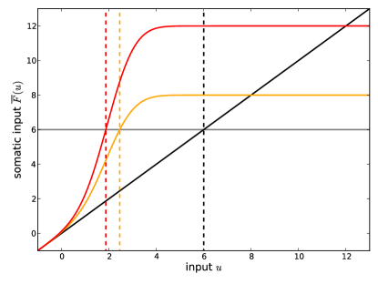
Figure 3: Effective reduction of the neuronal threshold to $\vartheta\leq\Theta$ by nonlinear dendrites. The traditional, linear transfer function $u$ (solid black) crosses the threshold $\Theta=6$ (solid gray) at $\vartheta=6$ (dashed black). For $B=2$, $PN^{-1}\mathrm{Var}\left[w\right]=0.8$, and $\theta=1$, dendritic nonlinearities $\bar{F}\left(u\right)$ (Eq. (23)) with strengths $D=4$ (solid orange) and $D=6$ (solid red) lead to effective thresholds $\vartheta\approx 2.5$ (dashed orange) and $\vartheta\approx 1.9$ (dashed red), respectively.

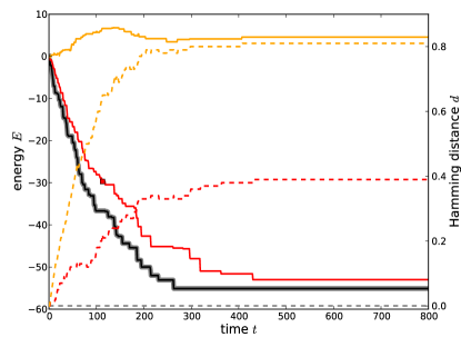
Figure 4: Network convergence with effective threshold reduction by nonlinear dendrites. Simulation of a network of $N=100$ binary neurons with $\Theta=0.4$, $B=2$, $P=8$, and $\mathrm{Var}\left[w\right]=0.1$. Simulations are performed with identical initial states, topology and identical realization of the (random) order of updates. The energy function (Eq. (15)) for linear input summation (solid black) decreases and the network converges towards a fixed point. Including weakly nonlinear branches (thick gray, $\theta=0.6$ and $D=1$) does not alter the dynamics or the energy of the modified network (which is now given by Eq. (27)). This is confirmed by the vanishing Hamming distance $d=\frac{1}{2N}\sum_{n=1}^{N}\left|v_{n}-v_{n}^{{}^{\prime}}\right|$ (dashed gray) between the two systems. For stronger dendritic spikes (solid red, $\theta=0.1$ and $D=2$), deviations of the somatic input from its ensemble average $\bar{F}$ and slightly asymmetric couplings lead to occasional increases in the energy (red square) but network convergence is preserved (checked for $1000$ runs). The dynamics converge towards an attractor that is different from that of the linear network as shown by the Hamming distance (dashed red) between the systems. When inhibitory and excitatory inputs are processed separately by the soma and the dendrites, respectively, no energy function is known and we exemplarily choose the energy function given by Eq. (27) with $\vartheta=\Theta$. The energy is then non-monotonic (solid orange, $\theta=0.1$ and $D=2$) but the system nonetheless reaches a stationary state (checked in simulations up to $t=2000$) which is different from the one of the linear system, cf. the Hamming distance (dashed orange).

How do nonlinear dendrites influence the dynamics of associative neural networks? Because of its analytical accessibility and its relevance in neural computation, we consider a Hopfield network Hopfield, (1982) of $N$ neurons $n\in\left\{1,\ldots,N\right\}$ with discrete states $v_{n}\in\left\{-1,+1\right\}$ and asynchronous updates of one random unit at a discrete time $t\in\mathbb{N}$. We might interpret $t$ as being measured in units of $N^{-1}\Delta t$ so that on average each neuron is updated once per $\Delta t$ ($\approx$ dendritic spike duration) and samples states which are present in other neurons for $\Delta t$ ($\approx$ dendritic integration window). The update rule for the conventional deterministic Hopfield model reads

$$v_{n}\left(t+1\right) = \mathrm{sign}\left[u_{n}\left(v_{1}\left(t\right),\dots,v_{N}\left(t\right)\right)-\Theta\right],$$ (13)

where $n$ is the neuron updated at $t$. $\mathrm{sign}$$\left(x\right)$, with $\mathrm{sign}\left(x\right)=-1$ if $x<0$ and $\mathrm{sign}\left(x\right)=1$ otherwise, is the neuronal transfer function and $\Theta$ denotes the neuronal threshold. $u_{n}$ is the linear field

$$u_{n}=u_{n}\left(v_{1},\ldots,v_{N}\right)=\sum_{m=1}^{N}w_{n,m}v_{m}.$$ (14)

The couplings $w_{n,m}$ between neurons $n$ and $m\in\left\{1,\ldots,N\right\}$ are assumed to be symmetric $w_{n,m}=w_{m,n}$. Then, a Lyapunov function may be derived,

$$E_{\mathrm{L}}\left(v_{1}\left(t\right),\dots,v_{N}\left(t\right)\right) = -\frac{1}{2}\sum_{n=1}^{N}\sum_{m=1}^{N}w_{n,m}v_{n}\left(t\right)v_{m}\left(t\right)$$ (15)

$$+\sum_{n=1}^{N}\Theta v_{n}\left(t\right),$$

satisfying $E_{\mathrm{L}}\left(t+1\right)\leq E_{\mathrm{L}}\left(t\right)$ Hopfield, (1982); Hertz et al., (1991). Equality $E_{\mathrm{L}}\left(t+1\right)=E_{\mathrm{L}}\left(t\right)$ only occurs if the state of the network upon update is not changed or in the rare case when $u_{n}$ matches exactly the threshold $\Theta$. Since $E_{\mathrm{L}}$ is bounded and $u_{n}=\Theta$ implies $v_{n}\left(t+1\right)=1$, the weak Lyapunov property guarantees convergence of the system. Thus, the network converges to an asymptotically stable minimum in the energy landscape $E_{\mathrm{L}}\left(v_{1},\dots,v_{N}\right)$.

To store $P$ patterns $\xi^{p}$, $p\in\left\{1,\dots,P\right\}$, the couplings in the Hopfield model are set in Hebbian manner Hebb, (1949),

$$w_{n,m} = N^{-1}\sum_{p=1}^{P}\xi_{n}^{p}\xi_{m}^{p}.$$ (16)

Classically, the storage of random, uncorrelated patterns $\xi_{n}^{p}\in\left\{-1,+1\right\}$ is studied, where $\xi_{n}^{p}=\pm 1$ with equal probabilities. Self-coupling terms $w_{n,n}$ may lead to spurious states close to stored patterns and are usually omitted, $w_{n,n}=0$Hertz et al., (1991). In this article we adopt these conventions.

An alternative and similarly common model represents the neuronal states via $v_{n}\in\left\{0,1\right\}$ (cf. e.g. Tsodyks and Feigel’man, (1988)). For an appropriate choice of variables (cf. Hertz et al., (1991)) this is equivalent to the $\left\{-1,+1\right\}$-model, when introducing a dependence of the neuronal threshold $\Theta$ on the couplings $w_{nm}$. Since we assume constant Hebbian couplings (Eq. (16)), we can include this term into the (then still constant) thresholds and translate a $\left\{0,1\right\}$-model into a $\left\{-1,+1\right\}$-model. Because it is most often used in classical statistical mechanics studies of neural networks (cf. Amit et al., 1985b ), we adopt the $\left\{-1,+1\right\}$-representation.

We now modify this well-known model to incorporate dendritic branches. For simplicity, we assume that each neuron has $B$ dendritic branches. The arborization changes the network topology (Fig. 1) since neurons are now linked to branches. The coupling matrix becomes a $N\times B\times N$-“matrix” with entries $w_{n,b,m}$ that characterize the coupling of neuron $m$ to branch $b$ of neuron $n$. The input to an individual dendrite is given by the dendritic field

$$u_{n,b}=u_{n,b}\left(v_{1},\ldots,v_{N}\right)=\sum_{m=1}^{N}w_{n,b,m}v_{m}.$$ (17)

The inputs are processed by the dendrites according to Eq. (1) and the somatic input is given by Eq. (6). Taken together, the update rule at time $t$ reads

$$v_{n}\left(t+1\right) = \mathrm{sign}\left[G_{n}\left(v_{1}\left(t\right),\dots,v_{N}\left(t\right)\right)-\Theta\right],$$ (18)

where

$$G_{n} =G_{n}\left(v_{1},\ldots,v_{N}\right)$$

$$=F\left(u_{n,1}\left(v_{1},\ldots,v_{N}\right),\ldots,u_{n,B}\left(v_{1},\ldots,v_{N}\right)\right).$$ (19)

Like in the classical Hopfield model, we assume a Hebbian rule which strengthens connections $w_{n,b,m}$ between co-active neurons such that their expected value is $\mathrm{E}\left[w_{n,b,m}\right]=B^{-1}w_{n,m}$, with $w_{n,m}$ given by Eq. (16). Because the process of adjustment of synaptic weights is subject to fluctuations Graupner and Brunel, (2012), we further assume that the weights $w_{n,b,m}$ are distributed with variance $\mathrm{Var}\left[w_{n,b,m}\right]=w_{n,m}^{2}B^{-2}\mathrm{Var}\left[w\right]$. The width of the distribution is proportional to the mean (with a parameter $\mathrm{Var}\left[w\right]$) which avoids excessively large deviations for small weights.

The network is fully connected and because input correlations across branches vanish (App. A4), this setup can be identified with the binomial scenario introduced before, with $S=N$ and $p_{b}=p_{0}=1$. Eqs. (3) and(4) yield (App. A4)

$$\mathrm{E}\left[u_{n,b}\right] = B^{-1}u_{n},$$ (20)

$$\mathrm{Var}\left[u_{n,b}\right] = B^{-2}PN^{-1}\mathrm{Var}\left[w\right].$$ (21)

The moments are computed as ensemble averages over an ensemble of neurons with index $n$ at a fixed network state (annealed approximation). The neural identity is preserved as it is specified by the parameters $w_{n,m}$ that determine the expectation value and the variance of the weight distribution of $w_{n,b,m}$ over which we average. An averaging over $x_{b}$ is unnecessary as $p_{b}=p_{0}=1$, and thus $\mathrm{E}\left[x_{b}\right]=N$ and $\mathrm{Var}\left[x_{b}\right]=0$. The mean somatic input at neuron $n$, $\mathrm{E}\left[G_{n}\right]$, follows from Eqs. (7)-(9). It depends on $v_{1},\ldots,v_{N}$ and $n$ only via the mean input per branch (Eq. (20)), and thus via the linear field $u_{n}$ (Eq. (14)). We may therefore define an effective input function $\bar{F}=\bar{F}\left(u_{n}\right)$ as

$$\bar{F}\left(u_{n}\left(v_{1},\ldots,v_{N}\right)\right)=\mathrm{E}\left[G_{n}\left(v_{1},\ldots,v_{N}\right)\right].$$ (22)

From Eqs. (7)-(9) we find

$$\bar{F}\left(u_{n}\right) =BP_{\mathrm{NL}}D+\left(1-P_{\mathrm{NL}}\right)u_{n}-BC_{\mathrm{NL}}$$ (23)

with

$$P_{\mathrm{NL}} = \frac{1}{2}\mathrm{erfc}\left(\frac{B\theta-u_{n}}{\sqrt{2PN^{-1}\mathrm{Var}\left[w\right]}}\right),$$ (24)

$$C_{\mathrm{NL}} = B^{-1}\sqrt{\frac{P\mathrm{Var}\left[w\right]}{2\pi N}}\exp\left(-\frac{\left(B\theta-u_{n}\right)^{2}}{2PN^{-1}\mathrm{Var}\left[w\right]}\right).\,\,\,\,\,\,\,$$ (25)

Analogously,Eq. (11) shows that the standard deviation of $G_{n}$, $\mathrm{Std}\left[G_{n}\right]$, is a function of the mean input per branch only. We may therefore define $\mathrm{Std}\left[F\right]=\mathrm{Std}\left[F\left(u_{n}\right)\right]$ via $\mathrm{Std}\left[G_{n}\left(v_{1},\ldots,v_{n}\right)\right]=\mathrm{Std}\left[F\left(u_{n}\left(v_{1},\ldots,v_{n}\right)\right)\right]$ and compute it from Eqs. (11) and(23).

To investigate the convergence properties of the network, we consider its state $\left(v_{1}\left(t\right),\dots,v_{N}\left(t\right)\right)$ at time $t$ and the update of a neuron $n$ by Eq. (18). Led by Fig. 2, we neglect the fluctuations $\mathrm{Std}\left[F\right]\ll\bar{F}$ and replace $G_{n}$ in Eq. (18) by its mean $\bar{F}\left(u_{n}\right)$. This approximation of the response of neuron $n$ by the response of a typical neuron with identity $n$ (as specified by the weights $w_{n,m}$) simplifies the analysis of the network dynamics. For reasonable parameter choices, the deviations are small and lead to erroneous updates of neuron states very rarely (Fig. 4). Furthermore, we may assume that the effective input function $\bar{F}\left(u_{n}\right)$ is strictly monotonic in $u_{n}$ and thus invertible (App. A5). These dynamics are then equivalent to the conventional Hopfield network dynamics (Eqs. (13)-(15), see App. A5) with coupling matrix $w_{n,m}$ and an effective threshold $\vartheta$. $\vartheta$ is determined by the intersection of the effective somatic input $\bar{F}$ and the neuronal threshold $\Theta$ (Fig. 3),

$$\vartheta=\bar{F}^{-1}\left(\Theta\right).$$ (26)

In particular, for symmetric weights, $w_{n,m}=w_{m,n}$, the dynamics has a Lyapunov function (App. A5)

$$E_{\mathrm{NL}}\left(v_{1}\left(t\right),\dots,v_{N}\left(t\right)\right) = -\frac{1}{2}\sum_{n=1}^{N}\sum_{m=1}^{N}w_{n,m}v_{n}\left(t\right)v_{m}\left(t\right)$$ (27)

$$+\sum_{n=1}^{N}\vartheta v_{n}\left(t\right).$$

By construction, $E_{\mathrm{NL}}$ decreases in time and the system converges towards a dynamical fixed point. Thus, the supralinear dendrites effectively reduce the neuronal threshold to $\vartheta\leq\Theta$ and leave the convergence properties of the system unchanged.

To study the convergence of the extended Hopfield model, we generate a network by first drawing Hebbian synaptic weights $w_{n,m}$ according to Eq. (16). This yields random patterns with $\xi_{n}^{p}=\pm 1$ with equal probabilities. Then, $w_{n,b,m}$ are drawn from a Gaussian distribution with mean $\mathrm{E}\left[w_{n,b,m}\right]=B^{-1}w_{n,m}$ and variance $\mathrm{Var}\left[w_{n,b,m}\right]=w_{n,m}^{2}B^{-2}\mathrm{Var}\left[w\right]$ as explained above. We note that generally $\sum_{b=1}^{B}w_{n,b,m}=:w_{n,m}^{{}^{\prime}}\neq w_{m,n}^{{}^{\prime}}$ so that the neuronal connectivity in presence of dendrites is not symmetric like in the classical Hopfield model. The energy function in Eq. (27) was derived for symmetric weights $w_{n,m}^{{}^{\prime}}=w_{n,m}=w_{m,n}=w_{m,n}^{{}^{\prime}}$ which may be seen as an approximation valid at least for slightly asymmetric couplings. Fig. 4 shows that this approximate energy function correctly reflects the convergence of the network. Also stronger deviations from the symmetric scenario (quantified by $\mathrm{Var}\left[w\right]$) leave the findings largely unchanged (App. A6).

The results of numerical simulations displayed in Fig. 4 illustrate the convergence properties of our model. If the threshold reduction by dendrites is small, subthreshold inputs to a neuron remain subthreshold also in the presence of nonlinear dendrites and the network converges to the same state as for linear branches (Fig. 4, gray). However, if the effective threshold reduction is stronger, inputs that are subthreshold may become superthreshold due to the dendritic nonlinearity and the same initial conditions tend to converge towards different attractors (Fig. 4, red). Since deviations of the somatic input from its ensemble average $\bar{F}$ may violate our approximation and the network is slightly asymmetric, the energy function can occasionally increase (Fig. 4, red square). However, for the considered parameters, these events occur rarely and do not affect the long-term convergence of the system (checked for $1000$ runs, not shown).

If inhibitory synapses project directly onto the soma instead of being mingled with excitatory synapses on the dendrites, the effective somatic input $\bar{F}$ is given by Eq. (12). Since the dendritic saturation by excitatory input may be exceeded by linear inhibition, $\bar{F}$ is non-monotonic and no Lyapunov function is apparent. The energy of the system as given by Eq. (27) with, e.g., $\vartheta=\Theta$ does not decrease monotonically in time (Fig. 4, orange). However, numerical simulations suggest that the network reaches a stable fixed point nevertheless, as exemplarily shown in Fig. 4. Such network convergence despite non-monotonic transfer functions is known from other systems Hirsch, (1989); Morita, (1993); Inoue, (1996). These studies do not split excitation and inhibition but choose transfer functions non-monotonic in the total, linear input $u_{n}$.

II.5 Capacity of stochastic Hopfield networks with non-additive dendritic input processing

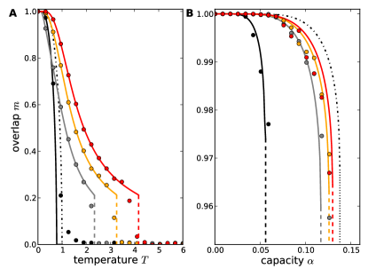
Figure 5: Non-additive dendritic coupling increases the overlap $m$ of the network state with a retrieval pattern. Simulation results (circles) and analytical results (solid lines) for linear (black) and nonlinear summation with dendritic spike strengths $D\in\left\{0.4,0.6,0.8\right\}$ (gray, orange, red). The remaining parameters are $N=4000$, $B=2$, $\theta=0.1$, $\Theta=0.4$, and $\mathrm{Var}\left[w\right]=0.1$. Results for linear input summation with $\Theta=0$ are included for comparison (dash-dotted black). The setup of the networks is the same as described in the discussion of Fig. 4. Panel (A) shows the overlap $m$ versus the temperature $T$ for a small load $\alpha=N^{-1}\approx 0$. It decreases with increasing $T$ and reaches zero at the critical temperature $T_{c}$ above which retrieval fails. This phase transition is discontinuous for the nonlinear and continuous for the linear model of input processing. Dendritic nonlinearities increase $T_{c}$. Panel (B) shows $m$ versus $\alpha$ at zero temperature $T=0$. It decreases with increasing load $\alpha$ and displays a discontinuous jump to zero at the critical storage capacity $\alpha_{c}$. $\alpha_{c}$ increases with stronger dendritic nonlinearities up to a level at which the effective threshold $\vartheta$ vanishes and the linear scenario with $\Theta=0$ is approached (dash-dotted black).

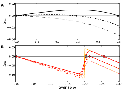
Figure 6: Graphical solutions to the transcendental equation for the overlap $m$ and phase transitions. Parameters are the same as in Fig. 5, with $D=0.4$. Eq. (30) is solved graphically, with its solutions given by the zero-crossings of $\Delta m$, i.e. the intersections with the solid gray line. For the traditional Hopfield case with linear input summation (A), the stable solution for the overlap $m$ continuously decreases (black markers, rectangle to circle to diamond) with increasing temperatures $T\in\left\{0.7,0.75,0.8\right\}$ (solid, dashed, dotted black) and reaches $m_{c}=0$ (diamond) at a critical value of $T_{c}\approx 0.8$. For nonlinear input summation due to nonlinear dendrites and small $\alpha=N^{-1}\approx 0$, panel (B) shows that increasing temperatures $T\in\left\{2.0,2.295,2.6\right\}$ (solid, dashed, dotted red) lead to decreasing overlaps $m$ (red markers, from rectangle to circle to diamond) which jump discontinuously from $m_{c}\approx 0.22$ (circle) to zero at $T_{c}\approx 2.3$. The gray rectangle indicates an unstable solution. In the limit $\alpha=0$ (B, orange), the jump in $\Delta m$ is discontinuous, which slightly changes the critical temperature but leaves the system’s critical behavior unchanged.

We now assess the extent to which a network of binary neurons with nonlinear dendrites is capable of storing and retrieving specific patterns. Since biological neurons are noisy, i.e. their input-output relation is not fully reliable (e.g. Smetters and Zador, (1996)), we generalize the above deterministic dynamics to allow for stochasticity. For the analysis of the storage capacity of the extended Hopfield network, we exploit the analogy between spin glasses and neural networks and employ statistical physics methods Amit et al., 1985a ; Hertz et al., (1991).

As a generalization of the deterministic update rule (Eq. (18)) we use the common Glauber dynamics Glauber, (1963); Shiino, (1990); Hertz et al., (1991) with asynchronous updates according to which the state of a randomly chosen neuron $n$ is set to $v_{n}=\pm 1$ with probability

$$p_{n}\left(v_{n}\right) = \left(1+\exp\left(-2\beta\left[G_{n}-\Theta\right]v_{n}\right)\right)^{-1}.$$ (28)

This is equivalent to flipping the state of the respective neuron with probability $p_{n}\left(v_{n}\rightarrow-v_{n}\right)=\left(1+\exp\left(2\beta\left[G_{n}-\Theta\right]v_{n}\right)\right)^{-1}$. Here, $T:=\beta^{-1}$ is the pseudo-temperature and a measure for the noise in the system and $G_{n}$ (Eq. (19)) is the input to the neuron. We recall that $P$ is the number of desired patterns and the fraction $\alpha=PN^{-1}$ is called load parameter. We obtain a temporally averaged state $\left\langle v_{n}\right\rangle$ of unit $n$ in the ensemble-averaged, stochastic network in mean-field theory by replacing $G_{n}$ by the ensemble average $\bar{F}\left(u_{n}\right)$ (Eq. (23)). Further, we replace the fluctuating argument of $\bar{F}\left(u_{n}\right)$ by its average, which yields $\bar{F}\left(\left\langle u_{n}\right\rangle\right)$, such that in the stationary state

$$\left\langle v_{n}\right\rangle = \left(+1\right)p_{n}\left(+1\right)+\left(-1\right)p_{n}\left(-1\right)$$ (29)

$$= \tanh\left(\beta\bar{F}\left(\left\langle u_{n}\right\rangle\right)-\beta\Theta\right)$$

$$= \tanh\left(\beta\bar{F}\left(N^{-1}\sum_{m=1}^{N}w_{n,m}\left\langle v_{m}\right\rangle\right)-\beta\Theta\right).$$

The overlap between pattern $p$ and state $\left\langle v_{n}\right\rangle$ is defined by $m^{p}:=N^{-1}\sum_{n=1}^{N}\xi_{n}^{p}\left\langle v_{n}\right\rangle$. Without loss of generality we study the retrieval of pattern $p=1$, so that $m:=m^{1}$ estimates the quality of retrieval. $m$ is given as an implicit solution to a set of coupled integral equations (App. A7, Eqs. (A7.3), (A7.6), (A7.8), and(A7.9)). In particular, we consider two limits, $\alpha\approx 0$ and $T=0$.

First, we study a finite number of patterns $P$ so that in the thermodynamic limit of large $N$ we have $\alpha\approx 0$ (App. A8). The overlap $m$ is given by the zeros of $\Delta m$,

$$\Delta m := \frac{1}{2}\tanh\biggl{(}\beta(1-P_{\mathrm{NL}}\left(m\right))m$$ (30)

$$+\beta\left(BDP_{\mathrm{NL}}\left(m\right)-BC_{\mathrm{NL}}\left(m\right)-\Theta\right)\biggr{)}$$

$$+\frac{1}{2}\tanh\biggl{(}\beta(1-P_{\mathrm{NL}}\left(-m\right))m$$

$$-\beta\left(BDP_{\mathrm{NL}}\left(-m\right)-BC_{\mathrm{NL}}\left(-m\right)-\Theta\right)\biggr{)}-m,\,\,\,\,$$

where the functions $P_{\mathrm{NL}}$ and $C_{\mathrm{NL}}$ are given by Eqs. (24) and(25). The solutions of the transcendental equation $\Delta m=0$ are obtained numerically and compared to simulation results of the Hopfield network with nonlinear dendrites (Fig. 5A).

The dendritic nonlinearities have a strong impact on the overlap curve. They change its shape and increase the critical temperature $T_{c}$ which marks the transition between functioning and non-functioning associative memory. They provide a discontinuous, first order phase transition with a non-zero critical overlap $m_{c}:=m\left(T_{c}\right)$. For the same parameters, the conventional Hopfield model displays a continuous, second order phase transition. These findings may be understood by graphically solving Eq. (30): For the considered, not too large $\Theta$ ($\Theta<0.448$), linear input processing leads to a concave $\Delta m\left(m\right)$ for high temperatures, so that the overlap continuously goes to zero when $T$ approaches the critical temperature $T_{c}$ (Fig. 6A). In the presence of nonlinear dendrites, we need to take into account that $PN^{-1}\mathrm{Var}\left[w\right]\propto\alpha\gtrsim 0$ (Eqs. (23)-(25)) is small so that the dendritic nonlinearity $\bar{F}$ sharply rises to its maximal (saturation) value at $m$ with $B\theta-m\approx 0$ due to its dependence on $P_{\mathrm{NL}}\left(m\right)$ (cf. Eq. (24) with $u_{n}=m$; $C_{\mathrm{NL}}\left(m\right)\propto\alpha$ is small). The second$\tanh$ is approximately constant there (because $P_{\mathrm{NL}}\left(-m\right)$ and $C_{\mathrm{NL}}\left(-m\right)$ are small for small $PN^{-1}\mathrm{Var}\left[w\right]$) and may be neglected. The sharp rise in $\bar{F}$ thus induces a convex turn in the right-hand side of Eq. (30) and results in a stable and an unstable fixed point of $m$ (Fig. 6B, red). With growing temperature $T$, the two fixed points vanish in a saddle-node bifurcation at non-zero $m_{c}\approx B\theta$ and the system undergoes a discontinuous phase transition of first order. For $\alpha=0$, the increase in $\bar{F}$ is jump-like so that no unstable fixed point appears and the critical overlap is $m_{c}=B\theta$ (Fig. 6B, orange).

The increased critical temperature $T_{c}$ due to the dendrites implies an increased robustness of the network against thermal fluctuations and may be intuitively understood as follows: If the network state is close to a learned pattern, the input to the neurons is either strongly positive and thus further amplified by the dendritic nonlinearities or strongly negative and not affected by the dendrites. The overall strengthening of the stored patterns counteracts the influence of the temperature (Eq. (28)) and stabilizes the patterns against thermal fluctuations. Consequently, the nonlinear dendrites allow pattern retrieval in a temperature regime in which linear neurons fail.

Because for the conventional Hopfield model neuronal thresholds $\Theta$ decrease the critical temperature (cf. Fig. 5A, black), we test if our results are a mere consequence of an effective threshold reduction, $\vartheta\leq\Theta$, by the nonlinear dendrites (cf. Eq. (26)). Repeating the above calculations and simulations with $\Theta=\vartheta=0$ we find that results as described above hold also for vanishing neuronal thresholds (App. A8).

Second, we consider the zero temperature limit $T=0$, in which thermal fluctuations cease and the binary neurons are deterministic threshold units (App. A9). The overlap $m$ is determined by

$$m = \frac{1}{2}\mbox{erf}\left(\frac{m-\vartheta}{\sqrt{2\alpha r}}\right)+\frac{1}{2}\mbox{erf}\left(\frac{m+\vartheta}{\sqrt{2\alpha r}}\right),$$

$$\sqrt{r} = 1+\sqrt{\frac{1}{2\pi\alpha}}\exp\left(-\frac{\left(m-\vartheta\right)^{2}}{2\alpha r}\right)$$ (31)

$$+\sqrt{\frac{1}{2\pi\alpha}}\exp\left(-\frac{\left(m+\vartheta\right)^{2}}{2\alpha r}\right),$$

where $\vartheta$ is the effective threshold (Eq. (26)). We solve these coupled equations numerically and compare them to the simulation data of a Hopfield network with nonlinear dendrites (Fig. 5B). Eqs. (31) are equivalent to the order parameter equations of the conventional Hopfield model with threshold $\vartheta$. For $\Theta>0$, we may therefore conclude that the dendritic branches reduce the neuronal threshold to $\vartheta\leq\Theta$ and thereby improve the critical storage capacity $\alpha_{c}$ of the network. Analogous to $T_{c}$, $\alpha_{c}$ denotes the critical load above which retrieval of patterns fails.

We note that the improved performance is a direct effect of the dendritic nonlinearity as demonstrated in Fig. 5, where the connectivity of neurons is the same for networks with linear and nonlinear dendrites while there is a clear increase in the critical temperature $T_{c}$ and load $\alpha_{c}$ in the latter case.

These findings may be understood by considering a neuronal threshold $\Theta\neq 0$ which generally introduces an asymmetry between the two states $v_{n}=\pm 1$ of a unit $n$. Since we assume the storage of random patterns $\xi_{n}^{p}=\pm 1$ with equal probabilities, the non-zero $\Theta\neq 0$ impedes the retrieval of learned patterns. For a positive threshold $\Theta>0$, the threshold reduction by the dendritic nonlinearities attenuates the asymmetry of the network and improves the retrieval of random patterns. In the zero temperature limit and for strong nonlinearities, our model becomes equivalent to the standard Hopfield model without threshold $\Theta=0$ (Fig. 5B, dash-dotted black).

We note that the agreement of analytical and numerical results as shown in Fig. 5 is even better if the couplings $w_{n,m}^{{}^{\prime}}=\sum_{b=1}^{B}w_{n,b,m}$ are normalized such that the $w_{n,m}^{{}^{\prime}}$ exactly equal the symmetric Hebbian weights $w_{n,m}$. This holds in particular for stronger dendritic spikes (Fig. 5B, red) which emphasize the asymmetry. To check if the above results hold also for larger deviations from the assumption of symmetric couplings, $w_{n,m}^{{}^{\prime}}=w_{m,n}^{{}^{\prime}}$, we repeat the simulations for larger $\mathrm{Var}\left[w\right]$ (cf. Eq. (21); App. A6). In the deterministic limit $T=0$ with many patterns, we find that stronger asymmetries impede the quality of retrieval. For finite temperatures $T>0$ and few patterns $\alpha\approx 0$, the impact of moderately asymmetric synaptic weights is negligible.

Complementing our analytical study of the limiting cases $\alpha\approx 0$ and $T=0$, we compute the quality of retrieval in the $\alpha$-$T$-phase space numerically. We find that our associative memory network with non-additive dendrites enables memory functioning in a larger $\alpha$-$T$-region than the model with linear branches (cf. App. A10).

II.6 Optimal number of dendritic branches for memory function

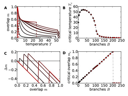
Figure 7: Memory performance in dependence of the number $B$ of dendritic branches. Parameters are the same as in Fig. 5, with $D=0.6$ and $\theta=0.005$. Branch numbers $B$ are color-coded from (black) to (red), cf. panels (B) and (D). Panels (A) and (C) show results for a few selected values of $B$. The overlap curves $m\left(T\right)$ with $\alpha\approx 0$ are computed for varying numbers $B$ of branches (A). The critical temperature $T_{c}$ depends non-monotonically on $B$ and is maximal for $B_{T,\mathrm{opt}}=30$ (B, dashed line and circles). For a fixed temperature, $T=25$, panel (C) shows $\Delta m$ whose zeros provide the solutions for $m$ (Eq. (30)) and whose maxima display a non-monotonical dependency on $B$. The critical overlap $m_{c}$ (D, dotted line and circles) grows approximately linearly with $B$ as indicated by the linear function $m_{c}=\theta B$ (D, solid line) and jumps to zero at $m_{c}\approx 1$.

Finally, we investigate the impact of varying numbers $B$ of dendritic branches on the performance of the extended stochastic Hopfield network. As shown above, non-additive dendritic input processing leads to an increased storage capacity and more robust memory retrieval by amplifying strong input to the neuron. Fig. 2B shows that, when this input is fixed, the average somatic input $\mathrm{E}\left[F\right]$ ($\hat{=}\bar{F}$) is maximal for an intermediate number of dendrites. This leads us to expect optimal memory performance for intermediate branch numbers.

We thus study the Hopfield network for varying $B$. In analogy to Fig. 5A we compute the overlaps $m$ for the limiting case $\alpha\approx 0$ (Fig. 7A). The critical temperature $T_{c}$ (Fig. 7B) displays a maximum at an intermediate number of branches, here $B_{T,\mathrm{opt}}=30$. For larger $\theta$, the optimal branch number is smaller (not shown). We can understand the maximum in $T_{c}$ by considering the $\Delta m\left(m\right)$ curves (Fig. 2C). They display maxima at $m_{c}\approx B\theta$ (see discussion of Fig. 6) with absolute heights determined by $m_{c}$ and $\bar{F}\left(m_{c}\right)$ where the latter is maximal for intermediate branch numbers. In combination, they yield the maxima of $\Delta m\left(m\neq 0\right)$ which are highest for intermediate numbers $B_{T,\mathrm{opt}}$ of branches. Upon increasing temperature, the corresponding curves are thus the last to fall entirely below zero at their $T_{c}\left(B\right)$ so that $T_{c}$ is highest for such branch numbers.

Another notable feature is the growing critical overlap $m_{c}$ at the critical temperature $T_{c}$ with increasing numbers of branches (Fig. 7D). As shown in the discussion of Fig. 6, the critical overlap for small $\alpha$ is given by $m_{c}\approx B\theta$. The argument is correct for strong nonlinearities $D$ and moderate $\theta B$ but breaks down for $\theta B\approx m_{c}>1$ since the overlap is naturally bounded by $1$ and only the solution $m_{c}=0$ remains, if a larger overlap would be needed to reach the upturn point of $\Delta m$ (cf. Fig. 7C). In particular, for large $B$, the behavior of the linear scenario with $m_{c}=0$ is reobtained.

Thus, the performance of the memory network depends non-trivially on the number of dendritic branches $B$. Additionally, depending on the purpose of the memory network, its robustness against noise (specified by $T_{c}$) may be balanced against the quality of retrieval (for which $m_{c}$ gives a worst-case measure) (cf. Fig. 7A).

III Conclusion: Nonlinear dendrites improve pattern retrieval

Non-additive processing of synaptic input is an important feature of biological neurons and may have severe consequences for neural processing in single neurons and networks. In this work, we first studied the influence of dendritic spikes in a neuron with a variable number of dendritic branches and sufficiently synchronous spiking input of variable strength, independently of a specific neuron model. We derived an approximation for the somatic input in the presence of nonlinear dendrites (Eqs. (7)-(10) and App. A3). This approximation allows the analytical investigation of dendritic summation phenomena in networks of arbitrary connectivity. Second, we extended the well-known Hopfield model to include neurons with branches that process inputs non-additively. Employing the results from the first part, we constructed networks which are, at each neuron, ensemble-averaged over the nonlinear dendrites and their inputs, such that the overall connectivity and thus the neural identities in the networks are preserved. These networks could be analyzed analytically with statistical physics methods. We used them to approximate the full dynamics of networks with nonlinear dendrites. We find that, for a deterministic Hopfield network, the dendritic nonlinearities reduce the neuronal thresholds (Eq. (26)) and the network still converges to a dynamical fixed point (Eq. (27)). Separate processing of inhibition and excitation (Eq. (12)) can break the monotonic decrease of common energy functions. A mean-field analysis for a stochastic Hopfield network revealed an improved memory storage capacity and a greater robustness against thermal fluctuations due to non-additive dendritic input processing (Eqs. (30) and (31) and App. A10). An intermediate number of dendritic branches was shown to optimally support memory functionality of the associative network.

Our findings help to advance the understanding of the role of nonlinear dendrites in three respects: (i) Earlier works studied the ability of arborized neurons to discriminate patterns Poirazi and Mel, (2001); Rhodes, (2008). They focused on a combinatorial approach of counting the numbers of different input-output functions of single neurons with multiple dendrites. In contrast, our study assumes a dynamical perspective. We derived an expression for the approximate somatic input which may be readily used to investigate the dynamics of networks of neurons with nonlinear dendrites for arbitrary connectivity and synaptic weights. (ii) We applied our results and studied the capability of networks with non-additive dendrites to serve as memory devices. Our work shows that nonlinear dendrites can increase the capacity and the robustness of memory retrieval against thermal fluctuations in recurrent, dynamic associative memory networks. (iii) Finally, our theoretical results suggest that there might be an intermediate number of dendritic branches that is optimal for network functionality Poirazi and Mel, (2001); Häusser and Mel, (2003). This may have severe implications for biological neural circuits featuring non-additive dendrites e.g. in the hippocampus. Since non-additive dendritic integration may take place in sliding window-like segments of the dendritic tree, a precise number of independent dendritic compartments is unlikely to be found Polsky et al., (2004). Biological studies suggest around $50-100$ independent sites capable of generating dendritic spikes per neuron, depending on the neuron type and function Elston and Rosa, (1998); Schiller and Schiller, (2001). Our model shows optimal memory performance for such numbers of branches, depending on the dendritic parameters (see discussion of Fig. 7).

For biological neural networks, we suggest that nonlinear dendrites may serve to stabilize memory recall against noisy network background activity. In such networks, memories might be stored in so-called Hebbian cell assemblies with higher internal connectivities or connection strengths that display elevated firing rates when presented with a specific input pattern Sommer and Wennekers, (2001); Aviel et al., (2005). Similar to our Hopfield model, matching patterns of activity provide a larger input to the other cells of the assembly which is amplified by the dendritic nonlinearities. In our model we restricted ourselves to Hebbian learning of coupling strengths, and noise and patterns were equally nonlinearly enhanced. Biological neural networks can change their wiring as well as the dendritic nonlinearities in an activity dependent manner Golding et al., (2002); Polsky et al., (2004); Losonczy et al., (2008). Further, some kinds of dendritic spikes amplify only temporally highly coordinated inputs Ariav et al., (2003). Both features may contribute to a selective nonlinear enhancement of pattern activity and may increase the stabilizing effects of non-additive dendrites in memory networks.

On a theoretical level of statistical physics, our work may be continued in several directions: Preliminary calculations suggest that for certain parameters new phenomena arise, such as improved memory retrieval for moderate noise levels (this is reminiscent of stochastic resonance Douglass et al., (1993); Kadar et al., (1998)). Further, previous studies on non-monotonic transfer functions found beneficial effects for memory performance in artificial and biological neural systems Hopfield, (1982); Morita, (1993); Inoue, (1996); Crespi, (1999). The novel kind of non-monotonicity which is due to dendritic reception of excitatory input and somatic reception of inhibitory input (cf. Eq. (12)) should be further explored and linked to these findings. Finally, many studies suggest that neural plasticity exploits dendritic spikes and dendritic compartmentalization Golding et al., (2002); Polsky et al., (2004); Losonczy et al., (2008). Non-Hebbian learning rules that are tailored to utilize dendritic spikes and branches were shown to increase the memory capabilities of single neurons or ensembles of such neurons Engel et al., (1992); Mel, 1992b ; Poirazi and Mel, (2001); Rhodes, (2008); Legenstein and Maass, (2011). Therefore, such dendrite-based learning is expected to boost also the performance of associative memory networks and is a particularly important target of future studies. Our statistical treatment (Eqs. (7)-(10)) and the numerical approach can be directly applied to address these issues. Gaining insight into these matters will help to better understand and utilize the full power of dendritic computation.

IV Acknowledgments

Supported by the BMBF (grant no. 01GQ1005B) and the DFG (grant no. TI 629/3-1). We thank Sven Jahnke and Gunter Weber for helpful discussions.

Appendix A1 Approximate mean and variance of the effective somatic input and the number of nonlinear branches

We compute the first moments of the somatic input $F$ (Eq. (6)) using a Gaussian approximation of the dendritic input distribution $P\left(u_{1},\dots,u_{B}\right)$ and assuming statistically identical branches, i.e. $p_{b}=p_{0}$, $b\in\left\{1,\dots,B\right\}$. Means $\mathrm{E}\left[u_{b}\right]$, variances $\mathrm{Var}\left[u_{b}\right]$ and covariances $\mathrm{Cov}\left[u_{b},u_{c}\right]$ of $P\left(u_{1},\dots,u_{B}\right)$ are given by Eqs. (3)-(5). We start with

$$\mathrm{E}\left[F\right] = \int_{-\infty}^{\infty}\mathrm{d}u_{1}\dots\int_{-\infty}^{\infty}\mathrm{d}u_{B}\left(f\left(u_{1}\right)+\dots+f\left(u_{B}\right)\right)P\left(u_{1},\dots,u_{B}\right)$$ (A1.1)

and pick $u:=u_{1}$ without loss of generality to obtain

$$\mathrm{E}\left[F\right] = B\int_{-\infty}^{\infty}\mathrm{d}uf\left(u\right)\int_{-\infty}^{\infty}\mathrm{d}u_{2}\dots\int_{-\infty}^{\infty}\mathrm{d}u_{B}P\left(u,u_{2,}\dots,u_{B}\right)$$ (A1.2)

$$= B\int_{-\infty}^{\infty}\mathrm{d}uf\left(u\right)P\left(u\right),$$

where $P\left(u\right)$ is the marginal distribution of $P\left(u,u_{2},\dots,u_{B}\right)$ and thus Gaussian with mean $\mathrm{E}\left[u\right]$ and variance $\mathrm{Var}\left[u\right]$. Using the definition of the dendritic transfer function $f$ (Eq. (1)), we split

$$\mathrm{E}\left[F\right] = B\left(\int_{\theta}^{\infty}\mathrm{d}uDP\left(u\right)+\int_{-\infty}^{\theta}\mathrm{d}uuP\left(u\right)\right)$$ (A1.3)

$$= BP_{\mathrm{NL}}D+B\left(1-P_{\mathrm{NL}}\right)\mathrm{E}\left[u\right]-BC_{\mathrm{NL}},$$

where we used partial integration in the second line and the definitions

$$P_{\mathrm{NL}} := \frac{1}{2}\mathrm{erfc}\left(\frac{\theta-\mathrm{E}\left[u\right]}{\sqrt{2\mathrm{Var}\left[u\right]}}\right),$$ (A1.4)

$$C_{\mathrm{NL}} := \sqrt{\frac{\mathrm{Var}\left[u\right]}{2\pi}}\exp\left(-\frac{\left(\theta-\mathrm{E}\left[u\right]\right)^{2}}{2\mathrm{Var}\left[u\right]}\right).$$ (A1.5)

The second moment is computed similarly,

$$\mathrm{E}\left[F^{2}\right] = \int_{-\infty}^{\infty}\mathrm{d}u_{1}\dots\int_{-\infty}^{\infty}\mathrm{d}u_{B}\left(f\left(u_{1}\right)+\dots+f\left(u_{B}\right)\right)^{2}P\left(u_{1},\dots,u_{B}\right)$$ (A1.6)

$$= B\int_{-\infty}^{\infty}\mathrm{d}uf^{2}\left(u\right)P\left(u\right)+\left(B^{2}-B\right)\int_{-\infty}^{\infty}\mathrm{d}u\int_{-\infty}^{\infty}\mathrm{d}vf\left(u\right)f\left(v\right)P\left(u,v\right)$$

$$= B\left(\int_{\theta}^{\infty}\mathrm{d}uD^{2}P\left(u\right)+\int_{-\infty}^{\theta}\mathrm{d}uu^{2}P\left(u\right)\right)$$

$$+\left(B^{2}-B\right)\Biggl{(}\int_{\theta}^{\infty}\mathrm{d}u\int_{\theta}^{\infty}\mathrm{d}vD^{2}P\left(u,v\right)$$

$$+2\int_{\theta}^{\infty}\mathrm{d}u\int_{-\infty}^{\theta}\mathrm{d}vDuP\left(u,v\right)+\int_{-\infty}^{\theta}\mathrm{d}u\int_{-\infty}^{\theta}\mathrm{d}vuvP\left(u,v\right)\Biggr{)}$$

$$= BP_{\mathrm{NL}}D^{2}+B\left(1-P_{\mathrm{NL}}\right)\left(\mathrm{E}^{2}\left[u\right]+\mathrm{Var}\left[u\right]\right)-BC_{\mathrm{NL}}\left(\mathrm{E}\left[u\right]+\theta\right)$$

$$+\left(B^{2}-B\right)I_{F}.$$

Here, $v:=u_{2}$ and the marginal distribution $P\left(u,v\right)$ is again Gaussian with means $\left(\mathrm{E}\left[u\right],\mathrm{E}\left[v\right]\right)$, variances $\left(\mathrm{Var}\left[u\right],\mathrm{Var}\left[v\right]\right)$ and covariance $\mathrm{Cov}\left[u,v\right]$. For binomially distributed numbers of active synapses per branch, $P\left(u,v\right)=P\left(u\right)P\left(v\right)$ and therefore

$$I_{F} = \left(P_{\mathrm{NL}}D\right)^{2}+2\left(P_{\mathrm{NL}}D\right)\left(\left(1-P_{\mathrm{NL}}\right)\mathrm{E}\left[u\right]-C_{\mathrm{NL}}\right)+\left(\left(1-P_{\mathrm{NL}}\right)\mathrm{E}\left[u\right]-C_{\mathrm{NL}}\right)^{2}$$ (A1.7)

$$= \left(P_{\mathrm{NL}}D+\left(1-P_{\mathrm{NL}}\right)\mathrm{E}\left[u\right]-C_{\mathrm{NL}}\right)^{2}$$

$$= \left(B^{-1}\mathrm{E}\left[F\right]\right)^{2}.$$

For a multinomial distribution of active synapses across branches, the double integral $I_{F}$ needs to be computed numerically (see Fig. 2).These results are discussed in the main text and in the caption to Fig. 2. The calculations may be easily extended to cover non-uniform branch probabilities $p_{b}$, dendritic thresholds $\theta_{b}$, and strengths $D_{b}$.

Similar to $\mathrm{E}\left[F\right]$, we compute the expected number $\mathrm{E}\left[k\right]$ of branches $k$ in the nonlinear regime. The dendritic transfer function $f\left(u\right)$ in Eq. (A1.1) is replaced by a step function $\mathrm{step}\left(u-\theta\right)$ to count the number of branches above threshold $\theta$. Here, we defined $\mathrm{step}\left(x\right)=0$ if $x<0$ and $\mathrm{step}\left(x\right)=1$ otherwise. Then,

$$\mathrm{E}\left[k\right] = \int_{-\infty}^{\infty}\mathrm{d}u_{1}\dots\int_{-\infty}^{\infty}\mathrm{d}u_{B}\left(\mathrm{step}\left(u_{1}-\theta\right)+\dots+\mathrm{step}\left(u_{B}-\theta\right)\right)P\left(u_{1},\dots,u_{B}\right)$$ (A1.8)

$$= B\int_{\theta}^{\infty}\mathrm{d}uP\left(u\right)$$

$$= BP_{\mathrm{NL}}.$$

Since the step function satisfies $\mathrm{step}^{2}\left(x\right)=\mathrm{step}\left(x\right)$ we derive the second moment of the distribution of the number $k$ of nonlinear branches via

$$\mathrm{E}\left[k^{2}\right] = \int_{-\infty}^{\infty}\mathrm{d}u_{1}\dots\int_{-\infty}^{\infty}\mathrm{d}u_{B}\left(\mathrm{step}\left(u_{1}-\theta\right)+\dots+\mathrm{step}\left(u_{B}-\theta\right)\right)^{2}P\left(u_{1},\dots,u_{B}\right)$$ (A1.9)

$$= B\int_{\theta}^{\infty}\mathrm{d}uP\left(u\right)+\left(B^{2}-B\right)\int_{\theta}^{\infty}\mathrm{d}u\int_{\theta}^{\infty}\mathrm{d}vP\left(u,v\right)$$

$$= BP_{\mathrm{NL}}+\left(B^{2}-B\right)I_{k}.$$

The binomial distribution of synapses among branches provides $P\left(u,v\right)=P\left(u\right)P\left(v\right)$ and thus

$$I_{k} = P_{\mathrm{NL}}^{2}=\left(B^{-1}\mathrm{E}\left[k\right]\right)^{2},$$ (A1.10)

while $I_{k}$ needs to be computed numerically in the multinomial case.

Appendix A2 Exact mean and variance of the effective somatic input and the number of nonlinear branches

We now derive the mean somatic input $\mathrm{E}\left[F\right]$ and its variance $\mathrm{Var}\left[F\right]$ for the exact distribution $P\left(u_{1},\dots,u_{B}\right)$ of input where $u_{b}=\sum_{i=1}^{x_{b}}w_{i}$ (cf. Eq. (2)) with Gaussian $P\left(w\right)$. We decompose $P\left(u_{1},\dots,u_{B}\right)$ into

$$P\left(u_{1},\dots,u_{B}\right) = \sum_{x_{1}=1}^{S}\dots\sum_{x_{B}=1}^{S}P\left(u_{1},\dots,u_{B}\mid x_{1},\dots,x_{B}\right)P\left(x_{1},\dots,x_{B}\right),$$ (A2.1)

where

$$P\left(u_{1},\dots,u_{B}\mid x_{1},\dots,x_{B}\right) = P\left(u_{1}\mid x_{1}\right)\cdots P\left(u_{B}\mid x_{B}\right)$$ (A2.2)

since $u_{b}$ depends only on $x_{b}$. The $P\left(u_{b}\mid x_{b}\right)$ are Gaussian distributed with means $x_{b}\mathrm{E}\left[w\right]$ and variances $x_{b}\mathrm{Var}\left[w\right]$ and $P\left(u_{1},\dots,u_{B}\right)$ is a weighted superposition of Gaussian distributions. For non-Gaussian $P\left(w\right)$ and large numbers of small inputs, we may employ a central limit theorem to establish Gaussianity of the $P\left(u_{b}\mid x_{b}\right)$. $\mathrm{E}\left[F\right]$ is computed as

$$\mathrm{E}\left[F\right] = \int_{-\infty}^{\infty}\mathrm{d}u_{1}\dots\int_{-\infty}^{\infty}\mathrm{d}u_{B}\left(f\left(u_{1}\right)+\dots+f\left(u_{B}\right)\right)P\left(u_{1},\dots,u_{B}\right)$$ (A2.3)

$$= \int_{-\infty}^{\infty}\mathrm{d}u_{1}\dots\int_{-\infty}^{\infty}\mathrm{d}u_{B}\sum_{b=1}^{B}f\left(u_{b}\right)\sum_{x_{1}=1}^{S}\dots\sum_{x_{B}=1}^{S}P\left(x_{1},\dots,x_{B}\right)P\left(u_{1},\dots,u_{B}\mid x_{1},\dots,x_{B}\right)$$

$$= \int_{-\infty}^{\infty}\mathrm{d}u_{1}\dots\int_{-\infty}^{\infty}\mathrm{d}u_{B}\sum_{b=1}^{B}f\left(u_{b}\right)\sum_{x_{1}=1}^{S}\dots\sum_{x_{B}=1}^{S}P\left(x_{1},\dots,x_{B}\right)P\left(u_{1}\mid x_{1}\right)\cdots P\left(u_{B}\mid x_{B}\right)$$

$$= \sum_{x_{1}=1}^{S}\dots\sum_{x_{B}=1}^{S}P\left(x_{1},\dots,x_{B}\right)\sum_{b=1}^{B}\int_{-\infty}^{\infty}\mathrm{d}u_{b}f\left(u_{b}\right)P\left(u_{b}\mid x_{b}\right)\prod_{c\neq b}^{B}\int_{-\infty}^{\infty}\mathrm{d}u_{c}P\left(u_{c}\mid x_{c}\right)$$

$$= \sum_{x_{1}=1}^{S}\dots\sum_{x_{B}=1}^{S}P\left(x_{1},\dots,x_{B}\right)\sum_{b=1}^{B}\int_{-\infty}^{\infty}\mathrm{d}u_{b}f\left(u_{b}\right)P\left(u_{b}\mid x_{b}\right)\cdot 1$$

$$= \sum_{x_{1}=1}^{S}\dots\sum_{x_{B}=1}^{S}P\left(x_{1},\dots,x_{B}\right)\sum_{b=1}^{B}\left[P_{\mathrm{NL},u_{b}\mid x_{b}}D+\left(1-P_{\mathrm{NL},u_{b}\mid x_{b}}\right)\mathrm{E}\left[u_{b}\mid x_{b}\right]-C_{\mathrm{NL},u_{b}\mid x_{b}}\right]$$

$$= \sum_{x=1}^{S}P\left(x\right)B\left[P_{\mathrm{NL},u\mid x}D+\left(1-P_{\mathrm{NL},u\mid x}\right)\mathrm{E}\left[u\mid x\right]-C_{\mathrm{NL},u\mid x}\right],$$

where we assumed identical statistics for all branches only in the last line and $P\left(x\right)$ is the marginal distribution of $P\left(x_{1},\dots,x_{B}\right)$. Similar to App. A1 we defined

$$P_{\mathrm{NL},u\mid x} := \frac{1}{2}\mathrm{erfc}\left(\frac{\theta-\mathrm{E}\left[u\mid x\right]}{\sqrt{2\mathrm{Var}\left[u\mid x\right]}}\right),$$ (A2.4)

$$C_{\mathrm{NL},u\mid x} := \sqrt{\frac{\mathrm{Var}\left[u\mid x\right]}{2\pi}}\exp\left(-\frac{\left(\theta-\mathrm{E}\left[u\mid x\right]\right)^{2}}{2\mathrm{Var}\left[u\mid x\right]}\right),$$ (A2.5)

with

$$\mathrm{E}\left[u\mid x\right] = x\mathrm{E}\left[w\right],$$ (A2.6)

$$\mathrm{Var}\left[u\mid x\right] = x\mathrm{Var}\left[w\right].$$ (A2.7)

The second moment of $F$ is given by

$$\mathrm{E}\left[F^{2}\right] = \int_{-\infty}^{\infty}\mathrm{d}u_{1}\dots\int_{-\infty}^{\infty}\mathrm{d}u_{B}\left(f\left(u_{1}\right)+\dots+f\left(u_{B}\right)\right)^{2}P\left(u_{1},\dots,u_{B}\right)$$ (A2.8)

$$= \sum_{x_{1}=1}^{S}\dots\sum_{x_{B}=1}^{S}P\left(x_{1},\dots,x_{B}\right)\sum_{b=1}^{B}\int_{-\infty}^{\infty}\mathrm{d}u_{b}f^{2}\left(u_{b}\right)P\left(u_{b}\mid x_{b}\right)$$

$$+\sum_{x_{1}=1}^{S}\dots\sum_{x_{B}=1}^{S}P\left(x_{1},\dots,x_{B}\right)\sum_{c=1}^{B}\sum_{b\neq c}^{B}\int_{-\infty}^{\infty}\mathrm{d}u_{b}\int_{-\infty}^{\infty}\mathrm{d}u_{c}f\left(u_{b}\right)f\left(u_{c}\right)P\left(u_{b}\mid x_{b}\right)P\left(u_{c}\mid x_{c}\right)$$

$$= \sum_{x=1}^{S}P\left(x\right)B\left[P_{\mathrm{NL},u\mid x}D^{2}+\left(1-P_{\mathrm{NL},u\mid x}\right)\left(\mathrm{E}^{2}\left[u\mid x\right]+\mathrm{Var}\left[u\mid x\right]\right)-C_{\mathrm{NL},u\mid x}\left(\mathrm{E}\left[u\mid x\right]+\theta\right)\right]$$

$$+\sum_{x=1}^{S}\sum_{y=1}^{S}P\left(x,y\right)\left(B^{2}-B\right)\left[P_{\mathrm{NL},u\mid x}D+\left(1-P_{\mathrm{NL},u\mid x}\right)\mathrm{E}\left[u\mid x\right]-C_{\mathrm{NL},u\mid x}\right]$$

$$\,\,\,\,\,\,\,\,\,\,\,\,\,\,\,\,\,\,\,\,\,\,\,\,\,\,\,\,\,\,\,\,\,\,\,\,\,\,\,\,\,\,\,\,\,\,\,\,\,\,\,\,\,\,\,\>\cdot\left[P_{\mathrm{NL},u\mid y}D+\left(1-P_{\mathrm{NL},u\mid y}\right)\mathrm{E}\left[u\mid y\right]-C_{\mathrm{NL},u\mid y}\right],$$

where the assumption of identical branch statistics was used in the last step and $P\left(x,y\right)$is the marginal distribution of $P\left(x_{1},\dots,x_{B}\right)$.

Analogously, we may compute the exact average number $\mathrm{E}\left[k\right]$ of nonlinear branches. Similar to App. A1, we use a step function to count the number $k$ of branches in the nonlinear regime,

$$\mathrm{E}\left[k\right] = \int_{-\infty}^{\infty}\mathrm{d}u_{1}\dots\int_{-\infty}^{\infty}\mathrm{d}u_{B}\left(\mathrm{step}\left(u_{1}-\theta\right)+\dots+\mathrm{step}\left(u_{B}-\theta\right)\right)P\left(u_{1},\dots,u_{B}\right)$$ (A2.9)

$$= \sum_{x=1}^{S}P\left(x\right)BP_{\mathrm{NL},u\mid x}.$$

The second moment yields

$$\mathrm{E}\left[k^{2}\right] = \int_{-\infty}^{\infty}\mathrm{d}u_{1}\dots\int_{-\infty}^{\infty}\mathrm{d}u_{B}\left(\mathrm{step}\left(u_{1}-\theta\right)+\dots+\mathrm{step}\left(u_{B}-\theta\right)\right)^{2}P\left(u_{1},\dots,u_{B}\right)$$ (A2.10)

$$= \sum_{x=1}^{S}P\left(x\right)BP_{\mathrm{NL},u\mid x}+\sum_{x=1}^{S}\sum_{y=1}^{S}P\left(x,y\right)\left(B^{2}-B\right)P_{\mathrm{NL},u\mid x}P_{\mathrm{NL},u\mid y}.$$

The exact expressions for $\mathrm{E}\left[F\right]$ and $\mathrm{Std}\left[F\right]=\sqrt{\mathrm{E}\left[F^{2}\right]-\mathrm{E}^{2}\left[F\right]}$ as well as $\mathrm{E}\left[k\right]$ and $\mathrm{Std}\left[k\right]=\sqrt{\mathrm{E}\left[k^{2}\right]-\mathrm{E}^{2}\left[k\right]}$ are compared to simulation results and the Gaussian approximation of $F$ (see App. A1) in Fig. 2.

Appendix A3 Effective somatic input approximation for neurons with multiple layers of dendritic branches

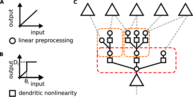
Figure A3.1: Neuron model with multiple layers of dendritic branches and non-additive processing. Similar to Fig. 1, different steps of linear (A) and non-additive dendritic input processing (B) are represented by circles and squares, respectively. A neuron with two levels of non-additive dendritic branches is displayed in (C). As exemplarily shown, the numbers of sub-branches may vary (at each level and between branches), and there may be synaptic input to linear and nonlinear dendrites at all levels.

The approximation for the somatic input $F$ (Eqs. (7)-(10)) may be readily employed to compute the somatic input for more complex dendritic arbors and multiple steps of non-additive dendritic processing (Fig. A3.1). For this, whenever necessary, we assume that the distribution of inputs may be approximated by the maximum entropy distribution for given mean and variance, i.e. by a normal distribution (cf. discussion of Eqs. (3)-(5)). For simplicity of presentation, we assume that the number of sub-branches $B_{l}$ at a level $l\in\left\{1,\dots,L\right\}$ is identical for all branches $b_{l}\in\left\{1,\dots,B_{l}\right\}$ at the level, that inputs arrive only at the terminal branches and sufficiently synchronously, and that the distribution of synapses is identical across the terminal branches. To compute the neuronal input for such a neuron, we may start from the soma and recursively work towards the terminal branches: The first moments of the effective somatic input are given by

$$\mathrm{E}\left[F\right] = B_{1}DP_{\mathrm{NL}}+B_{1}\left(1-P_{\mathrm{NL},1}\right)E\left[u_{1}\right]-B_{1}C_{\mathrm{NL},1},$$ (A3.1)

$$P_{\mathrm{NL},1} = P_{\mathrm{NL}}\left(\mathrm{E}\left[u_{1}\right],\mathrm{Var}\left[u_{1}\right]\right),$$ (A3.2)

$$C_{\mathrm{NL},1} = C_{\mathrm{NL}}\left(\mathrm{E}\left[u_{1}\right],\mathrm{Var}\left[u_{1}\right]\right),$$ (A3.3)

as defined in Eqs. (7)-(9) and $\mathrm{Var}\left[F\right]$ can be computed similarly, cf. Eq. (10). The appearing mean input per branch $\mathrm{E}\left[u_{1}\right]$ and its variance $\mathrm{Var}\left[u_{1}\right]$ are now given by an analogous approximation that captures the non-additive processing of the preceding layer. Indeed, the mean input per branch $E\left[u_{l-1}\right]$ for any layer $l-1$, $L\geq l>1$, is given by

$$\mathrm{E}\left[u_{l-1}\right] = B_{l}DP_{\mathrm{NL}}+B_{l}\left(1-P_{\mathrm{NL},l}\right)E\left[u_{l}\right]-B_{l}C_{\mathrm{NL},l},$$ (A3.4)

$$P_{\mathrm{NL},l} = P_{\mathrm{NL}}\left(\mathrm{E}\left[u_{l}\right],\mathrm{Var}\left[u_{l}\right]\right),$$ (A3.5)

$$C_{\mathrm{NL},l} = C_{\mathrm{NL}}\left(\mathrm{E}\left[u_{l}\right],\mathrm{Var}\left[u_{l}\right]\right),$$ (A3.6)

and $\mathrm{Var}\left[u_{l-1}\right]$ analogously, cf. Eq. (10). In this nomenclature, $\mathrm{E}\left[u_{0}\right]=\mathrm{E}\left[F\right]$ and $\mathrm{Var}\left[u_{0}\right]=\mathrm{Var}\left[F\right]$ capture the somatic input $F$, and $l=L$ indexes the layer of terminal branches which receives the synaptic input so that $E\left[u_{L}\right]=E\left[u\right]$ and $Var\left[u_{L}\right]=Var\left[u\right]$ (cf. Eqs. (3)-(5)). We note that one can also introduce factors implementing branch coupling strengths at this point.

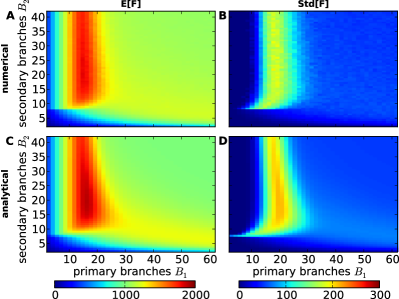
Figure A3.2: Somatic input for a neuron model with two layers of non-additive dendritic branches. Parameters are $\theta_{1}=100$, $D_{1}=200$, $\theta_{2}=5$, $D_{2}=10$, $\mathrm{E}\left[w\right]=1$, $\mathrm{Var}\left[w\right]=2$, and $S=1000$, synaptic input arrives at the terminal branches. Numerical results for the mean somatic input (A) and its standard deviation (B) for different numbers of branches on the first ($B_{1}$) and the second ($B_{2}$) level are obtained from $400$ realizations of multinomially distributed synapses. The corresponding analytical results from Eqs. (A3.3) and (A3.6) are highlighted in (C) and (D). Analytical and numerical results agree well. Input is largest for intermediate numbers of branches $B_{1,\mathrm{opt}}$ and $B_{2,\mathrm{opt}}$.

Fig. A3.2 shows good agreement of our analytical predictions with simulation results, both for the mean somatic input $\mathrm{E}\left[F\right]$ and its standard deviation $\mathrm{Std}\left[F\right]$. Dendritic thresholds and dendritic spike strengths in layer $l=1$ were increased to compensate for large input strengths in absence of branch coupling factors. We note that, as for the single-layered neuron, the input is largest for intermediate numbers of branches $B_{1,\mathrm{opt}}$ and $B_{2,\mathrm{opt}}$ (cf. discussion of Fig. 2).

The derivation can be directly generalized to cover non-identical branches, i.e. branches with different probabilities for the formation of synapses, different numbers of sub-branches (cf. App. A1 and A2), linear branches, and additional external inputs on intermediate level branches. To incorporate linear branches we may set the dendritic threshold to infinity, to incorporate external inputs to intermediate level dendrites, we can add an additional, linear input branch to the considered dendrite, where the external inputs arrive. We may thus conclude that our approach covers arbitrary tree-like dendritic structures.

Appendix A4 Mean and variance of the input per branch in a network with dendritic branches

We now derive the expected input to branch $b$ of neuron $n$ in the extended Hopfield model when the states of the neurons are fixed and the average is taken over the weight distribution. By construction, we have

$$\mathrm{E}\left[u_{n,b}\right] = \mathrm{E}\left[\sum_{m=1}^{N}w_{n,b,m}v_{m}\right]$$ (A4.1)

$$= \sum_{m=1}^{N}\mathrm{E}\left[w_{n,b,m}\right]v_{m}$$

$$= \sum_{m=1}^{N}B^{-1}w_{n,m}v_{m}$$

$$= B^{-1}u_{n},$$

so that the mean input to the branch depends only on the field $u_{n}$ of the classical Hopfield model. The choice $\mathrm{E}\left[w_{n,b,m}\right]=B^{-1}w_{n,m}$ in line three with $w_{n,m}$ given by Eq. (16) is justified by assuming Hebbian learning. The variance of the input per branch is given by

$$\mathrm{Var}\left[u_{n,b}\right] = \mathrm{Var}\left[\sum_{m=1}^{N}w_{n,b,m}v_{m}\right]$$ (A4.2)

$$= \sum_{m=1}^{N}v_{m}^{2}\mathrm{Var}\left[w_{n,b,m}\right]+\sum_{m\neq k}^{N}v_{m}v_{k}\mathrm{Cov}\left[w_{n,b,m},w_{n,b,k}\right]$$

$$= \sum_{m=1}^{N}\mathrm{Var}\left[w_{n,b,m}\right]+0$$

$$= \sum_{m=1}^{N}w_{n,m}^{2}B^{-2}\mathrm{Var}\left[w\right]$$

$$= \mathrm{Var}\left[w\right]B^{-2}N\mathrm{E}\left[w_{n,m}^{2}\right]$$

$$= \mathrm{Var}\left[w\right]B^{-2}N\left(\mathrm{Var}\left[w_{n,m}\right]+\mathrm{E}^{2}\left[w_{n,m}\right]\right),$$

where we used the independence of the $w_{n,b,m}$ in the third line. In the fourth line, we employed $\mathrm{Var}\left[w_{n,b,m}\right]=w_{n,m}^{2}B^{-2}\mathrm{Var}\left[w\right]$ with a parameter $\mathrm{Var}\left[w\right]$, cf. the discussion preceding Eqs. (20)-(21). For the Hopfield network with $P$ random patterns to be stored (Eq. (16)), $\mathrm{E}\left[w_{n,m}\right]=0$ and $\mathrm{Var}\left[w_{n,m}\right]=PN^{-2}=N^{-1}\alpha$ (with the load $\alpha=PN^{-1}$) since $w_{n,m}$ is a sum of $P$ contributions $\pm N^{-1}$ with equal probabilities. Finally, in our extended Hopfield model, the correlation of input between different branches vanishes,

$$\mathrm{Cov}\left[u_{n,b},u_{n,c}\right] = \mathrm{Cov}\left[\sum_{m=1}^{N}u_{n,b,m}v_{m},\sum_{k=1}^{N}u_{n,c,k}v_{k}\right]$$ (A4.3)

$$= \sum_{m=1}^{N}\sum_{k=1}^{N}v_{m}v_{k}\mathrm{Cov}\left[u_{n,b,m},u_{n,c,k}\right]$$

$$= 0,$$

where $b\neq c$. In the third line, we used that for $m=k$ the $u_{n,b,m}$ are independently chosen from (the same) Gaussian distributions with means $B^{-1}w_{n,m}$ and variances $B^{-2}w_{n,m}^{2}\mathrm{Var}\left[w\right]$ and for $m\neq k$ they are independently chosen from their respective (in general different) distributions. Because the input across branches is uncorrelated, we may employ the results for the somatic input we derived for binomially distributed active synapses (Eqs. (7) and (11)).

Appendix A5 Convergence of a Hopfield network with dendritic nonlinearities

Here, we show that the dynamics of the deterministic Hopfield network with nonlinear dendrites are equivalent to those of the classical Hopfield model with reduced threshold. In particular, network convergence is guaranteed. Assuming that $\bar{F}$ (Eq. (23)) is strictly monotonically increasing and therefore also invertible, we find that

$$v_{n}\left(t+1\right)=\mathrm{sign}\left(\bar{F}\left(u_{n}\left(t\right)\right)-\Theta\right) = \mathrm{sign}\left(u_{n}\left(t\right)-\vartheta\right),$$ (A5.1)

with the effective threshold

$$\vartheta = \bar{F}^{-1}\left(\Theta\right),$$ (A5.2)

see also Fig. 3. This update rule is equivalent to the conventional one with threshold $\vartheta$. Hence, the energy function $E_{\mathrm{NL}}$ of the system is obtained from $E_{\mathrm{L}}$ (Eq. (15)) by substituting $\Theta$ by $\vartheta$,

$$E_{\mathrm{NL}}\left(v_{1}\left(t\right),\dots,v_{N}\left(t\right)\right) = -\frac{1}{2}\sum_{n=1}^{N}\sum_{m=1}^{N}w_{n,m}v_{n}\left(t\right)v_{m}\left(t\right)+\sum_{m=1}^{N}\vartheta v_{m}\left(t\right).$$ (A5.3)

For symmetric couplings, $w_{n,m}=w_{m,n}$, $E_{\mathrm{NL}}$ is monotonically decreasing and the system converges to a steady state. More explicitly, by assuming that neuron $n$ is updated we have

$$E_{\mathrm{NL}}\left(t+1\right)-E_{\mathrm{NL}}\left(t\right) = -\left(v_{n}\left(t+1\right)-v_{n}\left(t\right)\right)\left(u_{n}\left(t\right)-\vartheta\right)\leq 0.$$ (A5.4)

Equality holds only for $v_{n}\left(t+1\right)=v_{n}\left(t\right)$ or $u_{n}\left(t\right)=\vartheta$ where the latter implies $v_{n}\left(t+1\right)=1$. Therefore, the energy $E_{\mathrm{NL}}$ either decreases in time or remains constant only if the state of the network does not change or the updated neuron $n$ is set to $v_{n}=1$. Since the energy is bounded from below due to

$$\left|E_{\mathrm{NL}}\right| \leq \frac{1}{2}\sum_{n=1}^{N}\sum_{m=1}^{N}\left|w_{n,m}\right|+N\vartheta,$$ (A5.5)

the network converges to a stable state which is given by a minimum in the energy landscape $E_{\mathrm{NL}}\left(v_{1},\dots,v_{N}\right)$. Thus, the effective nonlinearity reduces the neuronal threshold to $\vartheta\leq\Theta$ as compared to linear input summation (Eq. (15)) but maintains network convergence.

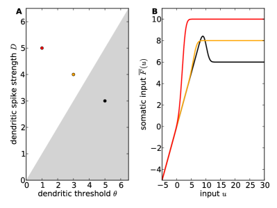
Figure A5.1: Monotonicity of the effective somatic input $\bar{F}$. Panel (A) indicates the monotonicity of $\bar{F}$ (Eq. (23)) for $B=2$, $PN^{-1}\mathrm{Var}\left[w\right]=0.8$ (cf. caption of Fig. 3) with varying dendritic thresholds $\theta$ and dendritic spike strengths $D$. It displays two regions, one where $\bar{F}$ is strictly monotonic (white) and one where it is non-monotonic (gray). They are separated by $D=\theta$. Panel (B) shows the monotonic or non-monotonic shape of $\bar{F}$ for different dendritic parameters $\left(\theta,D\right)\in\left\{\left(5,3\right),\left(3,4\right),\left(1,5\right)\right\}$ (black, orange, red).

For $\vartheta$ to be uniquely defined, the dendritic nonlinearities have to be strong enough, $BD>\Theta$, so that $\bar{F}$ intersects the constant function $\Theta$ (Fig. 3). Analytical calculations show that for $D>\theta$ the transfer function $\bar{F}$ is strictly monotonic (cf. Fig. A5.1). Since experiments demonstrate supralinear dendritic amplification, e.g., with thresholds of $\theta\approx 3.8\,\mathrm{mV}$ and spike amplitudes of $D\approx 10\,\mathrm{mV}$ Ariav et al., (2003), this parameter regime is biologically plausible.

Appendix A6 Asymmetric couplings and convergence of a Hopfield network with nonlinear dendrites

The couplings of the classical Hopfield network are symmetric, $w_{n,m}=w_{m,n}$, so that convergence is guaranteed by a Lyapunov function (Eq. (15)). In the extended model, we argued that the coupling weights $w_{n,b,m}$ to the dendritic branches obey $\mathrm{E}\left[w_{n,b,m}\right]=B^{-1}w_{n,m}$ or, equivalently, $B\mathrm{E}\left[w_{n,b,m}\right]=w_{n,m}$ due to Hebbian learning (Eq. (20)). To account for fluctuations in the learned weights we assumed a variance $\mathrm{Var}\left[w_{n,b,m}\right]=w_{n,m}^{2}B^{-2}\mathrm{Var}\left[w\right]$ (Eq. (21)). In a particular network realization with a finite number of branches and fluctuations, the dendritic weights do therefore not sum up to the expected Hebbian weight precisely,

$$\sum_{b=1}^{B}w_{n,b,m} =: w_{n,m}^{{}^{\prime}}\neq w_{n,m}.$$ (A6.1)

Generally, we have $w_{n,m}^{{}^{\prime}}\neq w_{m,n}^{{}^{\prime}}$ and the magnitude of the deviation from symmetric couplings is determined by $\mathrm{Var}\left[w\right]$. To check if our analytical calculations are applicable despite larger asymmetries, we redo the simulations from the main part of the paper for larger $\mathrm{Var}\left[w\right]$.

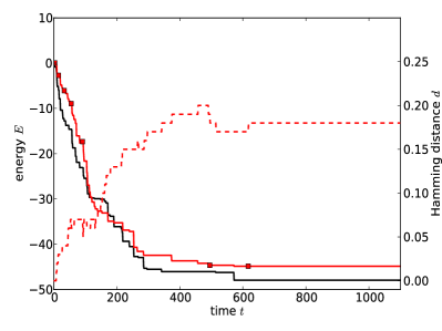
Figure A6.1: Network convergence despite more asymmetric couplings. Parameters are the same as in Fig. 4, with $\mathrm{Var}\left[w\right]=0.5$. Simulations are performed with identical initial states, topology and order of updates. As the linear Hopfield model is not affected by $\mathrm{Var}\left[w\right]$, its energy (solid black) decreases monotonically and reaches a fixed point. For the extended Hopfield model with non-additive dendrites and more asymmetric couplings, the energy decreases (solid red) with rare events of increasing energy (red squares) due to deviations from the mean-field approach or asymmetric couplings (cf. discussion of Eq. (27)). The convergence of the system is preserved (checked for $1000$ runs). The Hamming distance $d=\frac{1}{2N}\sum_{n=1}^{N}\left|v_{n}-v_{n}^{{}^{\prime}}\right|$ (dashed red) between the systems shows that they settle into different attractors.

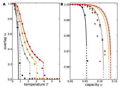
Figure A6.2: Memory performance of the stochastic Hopfield model with nonlinear dendritic branches and more asymmetric couplings. Parameters are the same as in Fig. 5, with $\mathrm{Var}\left[w\right]=0.5$. The figure compares analytical results (solid lines) for linear summation (black) and nonlinear summation with dendritic spike strengths $D\in\left\{0.4,0.6,0.8\right\}$ (gray, orange, red) and symmetric couplings to simulation results (circles) for asymmetric couplings. Results for linear input summation with $\Theta=0$ are included for comparison (dash-dotted black). Panel (A) shows the overlap $m$ versus the temperature $T$ for a small load $\alpha=N^{-1}\approx 0$. The more asymmetric couplings change $m$ only slightly and the simulation results agree well with the analytics of the symmetric couplings. Panel (B) shows $m$ versus $\alpha$ for $T=0$. The stronger asymmetries impair the memory function and the overlap $m$ displays a drop at lower loads $\alpha$ compared to the symmetric case.

Our simulations indicate that although convergence of the extended deterministic Hopfield network is not guaranteed by a Lyapunov function for asymmetric couplings, it reaches a fixed point as shown exemplarily by Fig. A6.1 and confirmed for $1000$ runs (not shown) also for larger asymmetries $\mathrm{Var}\left[w\right]$. To study the impact of asymmetric couplings on the memory performance of the extended stochastic Hopfield network, we repeat the simulations shown in Fig. 5 for larger $\mathrm{Var}\left[w\right]$. For a small load $\alpha\approx 0$ and non-zero temperatures $T>0$, the analytical calculations for symmetric couplings agree well with the simulation results (Fig. A6.2A). Yet, in the zero temperature limit $T=0$, the asymmetries decrease the storage capacity of the network compared to the symmetric case (Fig. A6.2B).

Appendix A7 Mean-field calculations for a stochastic Hopfield model with nonlinear dendritic branches

We now derive the mean-field equations for the overlap $m:=m^{1}=N^{-1}\sum_{n=1}^{N}\xi_{n}^{1}\left\langle v_{n}\right\rangle$ of the network state $\left(v_{1},\dots,v_{N}\right)$ with pattern $p=1$, i.e. $\left(\xi_{1}^{1},\dots,\xi_{N}^{1}\right)$. The following calculations go along those provided in Geszti, (1990); Hertz et al., (1991). From

$$\left\langle u_{n}\right\rangle = \sum_{k=1}^{N}w_{n,k}\left\langle v_{k}\right\rangle=\sum_{k=1}^{N}N^{-1}\sum_{p=1}^{P}\xi_{n}^{p}\xi_{k}^{p}\left\langle v_{k}\right\rangle=\sum_{p=1}^{P}\xi_{n}^{p}m^{p}=:u_{n}$$ (A7.1)

and Eq. (29) we find

$$m^{q} = N^{-1}\sum_{n=1}^{N}\xi_{n}^{q}\tanh\left[\beta\left(\bar{F}\left(u_{n}\right)-\Theta\right)\right]$$ (A7.2)

$$= N^{-1}\sum_{n=1}^{N}\xi_{n}^{q}\xi_{n}^{1}\tanh\left[\beta\xi_{n}^{1}\left(\bar{F}\left(u_{n}\right)-\Theta\right)\right],$$

where we employed the point symmetry of $\tanh\left(x\right)=-\tanh\left(-x\right)$ in the second line. We now assume that the number $P$ of patterns is large, of order $\mathcal{O}\left(N\right)$. We define the mean square overlap $r:=\alpha^{-1}\sum_{q\neq 1}^{P}\left(m^{q}\right)^{2}$ and assume that the $m^{q}$ are independent, zero-centered random variables with variance $\alpha rP^{-1}$. Then, the sum $\xi_{n}^{1}\sum_{p\neq 1}^{P}\xi_{n}^{p}m^{p}$ can be seen as a Gaussian noise term of variance $\alpha r$ and the sum $N^{-1}\sum_{n=1}^{N}$ may be treated as an average over this noise. Since $\xi_{n}^{1}=\pm 1$ with equal probabilities, the overlap with the first pattern is (Eq. (A7.2))

$$m = \frac{1}{2}\int_{-\infty}^{\infty}\frac{dz}{\sqrt{2\pi}}e^{-\frac{1}{2}z^{2}}\tanh\left[\beta\left(\bar{F}\left(m+\sqrt{\alpha r}z\right)-\Theta\right)\right]$$ (A7.3)

$$+\frac{1}{2}\int_{-\infty}^{\infty}\frac{dz}{\sqrt{2\pi}}e^{-\frac{1}{2}z^{2}}\tanh\left[-\beta\left(\bar{F}\left(-m-\sqrt{\alpha r}z\right)-\Theta\right)\right],$$

with the effective somatic input $\bar{F}$ given by Eqs. (23)-(25). Next,the correlations quantified by $r$ must be determined self-consistently. We define $\bar{u}_{n}^{q}:=\sum_{p\neq q}^{P}\xi_{n}^{p}m^{p}$ and because $\xi_{n}^{q}m^{q}=u_{n}-\bar{u}_{n}^{q}$ is small, of order $\mathcal{O}\left(N^{-1/2}\right)$, we expand Eq. (A7.2) into a Taylor series to first order,

$$m^{q} \approx N^{-1}\sum_{n=1}^{N}\xi_{n}^{q}\xi_{n}^{1}\tanh\left[\beta\xi_{n}^{1}\left(\bar{F}\left(\bar{u}_{n}^{q}\right)-\Theta\right)\right]$$ (A7.4)

$$+\beta N^{-1}\sum_{n=1}^{N}\left(1-\tanh^{2}\left[\beta\xi_{n}^{1}\left(\bar{F}\left(\bar{u}_{n}^{q}\right)-\Theta\right)\right]\right)\bar{F}^{{}^{\prime}}\left(\bar{u}_{n}^{q}\right)m^{q},$$

where $f^{{}^{\prime}}\left(x_{0}\right)=\left.\frac{df\left(x\right)}{dx}\right|_{x=x_{0}}$ denotes the first derivative of a function $f\left(x\right)$ evaluated at $x=x_{0}$. Similar to the derivation of Eq. (A7.3), we approximate $\xi_{n}^{1}\sum_{p\neq 1,q}^{P}\xi_{n}^{p}m^{p}$ by a zero-centered Gaussian distribution with variance $\alpha r$ and in the second term of Eq. (A7.4) treat the sum $N^{-1}\sum_{n=1}^{N}$ as an average so that

$$m^{q} = N^{-1}\sum_{n=1}^{N}\xi_{n}^{q}\xi_{n}^{1}\tanh\left[\beta\xi_{n}^{1}\left(\bar{F}\left(\bar{u}_{n}^{q}\right)-\Theta\right)\right]+\beta Cm^{q},$$ (A7.5)

with

$$C := \frac{1}{2}\int_{-\infty}^{\infty}\frac{dz}{\sqrt{2\pi}}e^{-\frac{1}{2}z^{2}}\left(1-\tanh^{2}\left[\beta\left(\bar{F}\left(m+\sqrt{\alpha r}z\right)-\Theta\right)\right]\right)\bar{F}^{{}^{\prime}}\left(m+\sqrt{\alpha r}z\right)$$ (A7.6)

$$+\frac{1}{2}\int_{-\infty}^{\infty}\frac{dz}{\sqrt{2\pi}}e^{-\frac{1}{2}z^{2}}\left(1-\tanh^{2}\left[-\beta\left(\bar{F}\left(-m-\sqrt{\alpha r}z\right)-\Theta\right)\right]\right)\bar{F}^{{}^{\prime}}\left(-m-\sqrt{\alpha r}z\right),\,\,\,\,\,\,\,\,\,\,\,\,\,\,$$

where we took into account again that $\xi_{n}^{1}=\pm 1$ with equal probabilities. Solving Eq. (A7.5) for $m^{q}$, squaring it and averaging over all patterns $q$ yields

$$r = \left(1-\beta C\right)^{-2}NP^{-1}\sum_{q\neq 1}^{P}N^{-2}\sum_{n,k=1}^{N}\xi_{n}^{q}\xi_{n}^{1}\xi_{k}^{q}\xi_{k}^{1}$$ (A7.7)

$$\cdot\tanh\left[\beta\xi_{n}^{1}\left(\bar{F}\left(\bar{u}_{n}^{q}\right)-\Theta\right)\right]\tanh\left[\beta\xi_{k}^{1}\left(\bar{F}\left(\bar{u}_{k}^{q}\right)-\Theta\right)\right]$$

$$= \left(1-\beta C\right)^{-2}N^{-1}\sum_{n=1}^{N}\tanh^{2}\left[\beta\xi_{n}^{1}\left(\bar{F}\left(\bar{u}_{n}^{2}\right)-\Theta\right)\right].$$

Here, we used that the arguments of the $\tanh$ are independent of $q$ and in the average $P^{-1}\sum_{q\neq 1}^{P}$ only terms $n=k$ survive. We set $\bar{u}_{n}^{q}=\bar{u}_{n}^{2}$ without loss of generality. Employing a Gaussian approximation of the sum $\xi_{n}^{1}\sum_{p\neq 1,2}^{P}\xi_{n}^{p}m^{p}$ like in Eq. (A7.5) yields

$$r = \left(1-\beta C\right)^{-2}s,$$ (A7.8)

with

$$s := \frac{1}{2}\int_{-\infty}^{\infty}\frac{dz}{\sqrt{2\pi}}e^{-\frac{1}{2}z^{2}}\tanh^{2}\left[\beta\left(\bar{F}\left(m+\sqrt{\alpha r}z\right)-\Theta\right)\right]$$ (A7.9)

$$+\frac{1}{2}\int_{-\infty}^{\infty}\frac{dz}{\sqrt{2\pi}}e^{-\frac{1}{2}z^{2}}\tanh^{2}\left[-\beta\left(\bar{F}\left(-m-\sqrt{\alpha r}z\right)-\Theta\right)\right].$$

The above Gaussian approximations hold for $\alpha$ of order $\mathcal{O}\left(1\right)$ and smaller. Eqs. (A7.3), (A7.6), (A7.8), and(A7.9) constitute a set of nonlinear, coupled integral equations for the order parameters $m$, $r$ and $s$ and can be solved numerically or in limiting cases.

Appendix A8 Memory capacity of a stochastic Hopfield network with nonlinear dendritic branches in the thermodynamic limit for a finite number of patterns

We now consider the quality of pattern retrieval estimated by the overlap $m$ in the thermodynamic limit of large $N$ with finitely many patterns $P$, i.e. $\alpha\approx 0$. Because $m^{q}$, $q\neq 1$, is of order $\mathcal{O}\left(N^{-1/2}\right)$ and $P$ is finite we may write $u_{n}=\sum_{p=1}^{P}\xi_{n}^{p}m^{p}\approx\xi_{n}^{1}m$. Starting from Eq. (A7.2) and using the definition of the effective somatic input $\bar{F}$ (Eqs. (23)-(25)),

$$m = N^{-1}\sum_{n=1}^{N}\tanh\left[\beta\left(1-P_{\mathrm{NL}}\left(u_{n}\right)\right)\xi_{n}^{1}u_{n}+\beta\xi_{n}^{1}\left(BDP_{\mathrm{NL}}\left(u_{n}\right)-BC_{\mathrm{NL}}\left(u_{n}\right)-\Theta\right)\right]$$ (A8.1)

$$\approx N^{-1}\sum_{n=1}^{N}\tanh\left[\beta\left(1-P_{\mathrm{NL}}\left(\xi_{n}^{1}m\right)\right)m+\beta\xi_{n}^{1}\left(BDP_{\mathrm{NL}}\left(\xi_{n}^{1}m\right)-BC_{\mathrm{NL}}\left(\xi_{n}^{1}m\right)-\Theta\right)\right]$$

$$= \frac{1}{2}\tanh\left[\beta\left(1-P_{\mathrm{NL}}\left(m\right)\right)m+\beta\left(BDP_{\mathrm{NL}}\left(m\right)-BC_{\mathrm{NL}}\left(m\right)-\Theta\right)\right]$$

$$+\frac{1}{2}\tanh\left[\beta\left(1-P_{\mathrm{NL}}\left(-m\right)\right)m-\beta\left(BDP_{\mathrm{NL}}\left(-m\right)-BC_{\mathrm{NL}}\left(-m\right)-\Theta\right)\right],$$

where we use that $\xi_{n}^{1}=\pm 1$ with equal probabilities in the third line. This transcendental equation for $m$ is solved numerically (Fig. 5).

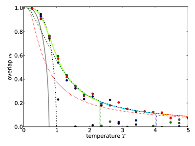
Figure A8.1: Critical behavior of the network for few patterns $\alpha\approx 0$ and varying neuronal thresholds $\Theta$ and dendritic thresholds $\theta$. Parameters are the same as in Fig. 5, with $D=0.4$ and different dendritic thresholds $\theta\in\left\{\infty,0.1,0.05,0\right\}$. Simulation results (circles) and analytical results (dash-dotted lines) for vanishing neuronal thresholds $\Theta=0$ are compared to the analytical results for $\Theta=0.4$ (solid lines; cf. Fig. 5). $\theta=\infty$ (dash-dotted black and solid gray) corresponds to the linear Hopfield model. Decreasing the dendritic threshold $\theta$ increases the critical temperature ($\theta=0.1$ in green and lime, $\theta=0.05$ in blue and cyan). For $\theta=0$ (red and orange), there is no phase transition anymore as $m\left(T\right)$ asymptotically follows Eq. (A8.2) (dotted red).

It is shown in the main text that dendritic nonlinearities elevate the critical temperature $T_{c}$ above which retrieval fails (Fig. 5). The increased critical temperature $T_{c}$ may result partially from the effectively reduced neuronal threshold $\vartheta\leq\Theta$ (Eq. (26)). To exclude this effect, we study the impact of the nonlinearity on the critical temperature $T_{c}$ for vanishing neuronal threshold $\Theta=0$. We find that when changing $\Theta$ from $\Theta=0.4$ to $\Theta=0$ the critical temperature $T_{c}$ is altered only slightly (Fig. A8.1, see differences between dashed and dotted vertical lines) and the behavior of the system remains the same.

In contrast, the threshold $\theta$ of the dendritic nonlinearity has a strong influence on the critical behavior of the network. For $\theta=\infty$, we reobtain linear input summation (Fig. A8.1, dash-dotted black and solid gray). For finite $0<\theta<\infty$, the critical temperature $T_{c}$ is increased (Fig. A8.1, green and lime, blue and cyan). For $\theta=0$, there is no phase transition at all (Fig. A8.1, red and orange) and memory retrieval at arbitrarily high temperatures $T$ (although with smaller and smaller overlaps$m$) is possible. This may be understood by assuming $\theta=0$ and $T=\beta^{-1}\rightarrow\infty$ in Eq. (A8.1). Then,

$$m \rightarrow \frac{1}{2}\tanh\left(T^{-1}\left(BD-\Theta\right)\right)+\frac{1}{2}\tanh\left(T^{-1}\Theta\right)$$ (A8.2)

because $P_{\mathrm{NL}}\left(m\right)\approx 1$ and $C_{\mathrm{NL}}\left(m\right)\approx P_{\mathrm{NL}}\left(-m\right)\approx C_{\mathrm{NL}}\left(-m\right)\approx 0$ for $\theta=0$ and $m\rightarrow 0$ for $T\rightarrow\infty$. Since $BD>\Theta$ (App. A5) we have $m>0$ for $T>0$ and no phase transition occurs (Fig. A8.1, dotted red).

Appendix A9 Memory capacity of a stochastic Hopfield network with nonlinear dendritic branches in the zero temperature limit

We now compute the overlap $m$ in the zero temperature limit $T=0$. Starting point are the Eqs. (A7.3), (A7.6), (A7.8), and(A7.9). For $\beta=T^{-1}\rightarrow\infty$, we may simplify

$$\lim_{\beta\rightarrow\infty}\tanh\left[\pm\beta\left(\bar{F}\left(\pm m\pm\sqrt{\alpha r}z\right)-\Theta\right)\right] = \mathrm{sign}\left[\pm\bar{F}\left(\pm m\pm\sqrt{\alpha r}z\right)\mp\Theta\right]$$ (A9.1)

$$= \mathrm{sign}\left[m+\sqrt{\alpha r}z\mp\vartheta\right],$$

by definition of the effective threshold $\vartheta$ (see Eq. (26)), $\bar{F}\left(\vartheta\right)=\Theta.$ Using the dominated convergence theorem, we may compute (Eq. (A7.3))

$$\lim_{\beta\rightarrow\infty}m = \frac{1}{2}\int_{-\infty}^{\infty}\frac{dz}{\sqrt{2\pi}}e^{-\frac{1}{2}z^{2}}\mathrm{sign}\left[m+\sqrt{\alpha r}z-\vartheta\right]$$ (A9.2)

$$+\frac{1}{2}\int_{-\infty}^{\infty}\frac{dz}{\sqrt{2\pi}}e^{-\frac{1}{2}z^{2}}\mathrm{sign}\left[m+\sqrt{\alpha r}z+\vartheta\right]$$

$$= \frac{1}{2}\mbox{erf}\left(\frac{m-\vartheta}{\sqrt{2\alpha r}}\right)+\frac{1}{2}\mbox{erf}\left(\frac{m+\vartheta}{\sqrt{2\alpha r}}\right)$$

and (Eq. (A7.9))

$$\lim_{\beta\rightarrow\infty}s = \frac{1}{2}\int_{-\infty}^{\infty}\frac{dz}{\sqrt{2\pi}}e^{-\frac{1}{2}z^{2}}\mathrm{sign}^{2}\left[m+\sqrt{\alpha r}z-\vartheta\right]$$ (A9.3)

$$+\frac{1}{2}\int_{-\infty}^{\infty}\frac{dz}{\sqrt{2\pi}}e^{-\frac{1}{2}z^{2}}\mathrm{sign}^{2}\left[m+\sqrt{\alpha r}z+\vartheta\right]$$

$$= 1.$$

To derive $r$, we further compute $\beta C$ (Eq. (A7.6)). We use that $\frac{\beta}{2}\left(1-\tanh^{2}\left[\beta x\right]\right)$ approaches the Dirac delta function $\delta\left(x\right)$ for $\beta\rightarrow\infty$,

$$\lim_{\beta\rightarrow\infty}\beta C = \int_{-\infty}^{\infty}\frac{dz}{\sqrt{2\pi}}e^{-\frac{1}{2}z^{2}}\delta\left[\bar{F}\left(m+\sqrt{\alpha r}z\right)-\Theta\right]\bar{F}^{{}^{\prime}}\left(m+\sqrt{\alpha r}z\right)$$ (A9.4)

$$+\int_{-\infty}^{\infty}\frac{dz}{\sqrt{2\pi}}e^{-\frac{1}{2}z^{2}}\delta\left[-\bar{F}\left(-m-\sqrt{\alpha r}z\right)+\Theta\right]\bar{F}^{{}^{\prime}}\left(-m-\sqrt{\alpha r}z\right)$$

$$= \frac{1}{\left|\bar{F}^{{}^{\prime}}\left(\vartheta\right)\right|\sqrt{\alpha r}}\int_{-\infty}^{\infty}\frac{dz}{\sqrt{2\pi}}e^{-\frac{1}{2}z^{2}}\delta\left[z+\frac{m-\vartheta}{\sqrt{\alpha r}}\right]\bar{F}^{{}^{\prime}}\left(m+\sqrt{\alpha r}z\right)$$

$$+\frac{1}{\left|\bar{F}^{{}^{\prime}}\left(\vartheta\right)\right|\sqrt{\alpha r}}\int_{-\infty}^{\infty}\frac{dz}{\sqrt{2\pi}}e^{-\frac{1}{2}z^{2}}\delta\left[z+\frac{m+\vartheta}{\sqrt{\alpha r}}\right]\bar{F}^{{}^{\prime}}\left(-m-\sqrt{\alpha r}z\right)$$

$$= \sqrt{\frac{1}{2\pi\alpha r}}\left[\exp\left(-\frac{\left(m-\vartheta\right)^{2}}{2\alpha r}\right)+\exp\left(-\frac{\left(m+\vartheta\right)^{2}}{2\alpha r}\right)\right].$$

In the second line we used $\delta\left(f\left(x\right)\right)=\left|f^{{}^{\prime}}\left(x_{0}\right)\right|^{-1}\delta\left(x-x_{0}\right)$ with the (single) root $x_{0}$, $f\left(x_{0}\right)=0$, and again $\bar{F}\left(\vartheta\right)=\Theta$. There and in the third line we used that $\bar{F}$ is monotonically increasing, i.e. $\bar{F}^{{}^{\prime}}\geq 0$. From Eqs. (A7.8) and(A9.4) we find

$$\sqrt{r} = 1+\sqrt{\frac{1}{2\pi\alpha}}\exp\left(-\frac{\left(m-\vartheta\right)^{2}}{2\alpha r}\right)+\sqrt{\frac{1}{2\pi\alpha}}\exp\left(-\frac{\left(m+\vartheta\right)^{2}}{2\alpha r}\right).$$ (A9.5)

Eqs. (A9.2) and(A9.5) provide coupled, implicit equations for the order parameters $m$ and $r$ which can be solved numerically. Solutions for varying effective thresholds $\vartheta$ are shown in Fig. 5.

Appendix A10 Phase diagrams of associative memory networks of neurons with additive and non-additive dendritic processing

For a further comparison of the memory performance of networks with arborized neurons with the classical Hopfield model, we compute the quality of retrieval $m$ in the $\alpha$-$T$-plane.

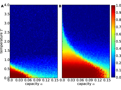
Figure A10.1: Quality of retrieval in dependence of capacity $\alpha$ and temperature $T$. Numerical results for the overlap $m$, averaged over $20$ realizations. Parameters are the same as in Fig. 5 with $D=0.8$. The network model with non-additive dendrites displays a larger region of stable memory retrieval (B) than the original Hopfield network (A).

We found both analytically and numerically that in the limits $\alpha\approx 0$ and $T=0$, the critical temperature and capacity of the network with non-additive dendrites are higher than for the linear model, cf. Fig. 5. Complementing these findings, numerical simulations show that the $\alpha$-$T$-region of successful memory retrieval is larger for non-additive dendrites (Fig. A10.1B) than for linear dendrites (Fig. A10.1A).

References

- Abeles, (1991) Abeles, M. (1991). Corticonics: Neural circuits of the cerebral cortex. Cambridge Univ. Pr., Cambridge.
- (2) Amit, Gutfreund, and Sompolinsky (1985a). Spin-glass models of neural networks. Phys Rev A, 32(2):1007–1018.
- (3) Amit, D. J., Gutfreund, H., and Sompolinsky, H. (1985b). Storing infinite numbers of patterns in a spin glass model of neural networks. Phys. Rev. Lett., 55:1530–1533.
- Ariav et al., (2003) Ariav, G., Polsky, A., and Schiller, J. (2003). Submillisecond precision of the input-output transformation function mediated by fast sodium dendritic spikes in basal dendrites of CA1 pyramidal neurons. J. Neurosci., 23(21):7750–7758.
- Aviel et al., (2005) Aviel, Y., Horn, D., and Abeles, M. (2005). Memory capacity of balanced networks. Neural Comput., 17(3):691–713.
- Barkai et al., (1990) Barkai, E., Hansel, D., and Kanter, I. (1990). Statistical mechanics of a multilayered neural network. Phys. Rev. Lett., 65(18):2310–2312.
- Biehl et al., (2000) Biehl, M., Ahr, M., and Schlösser, E. (2000). Statistical physics of learning: Phase transitions in multilayered neural networks. In Advances in Solid State Physics 40. Springer, Berlin.
- Blackwell and Girshick, (1946) Blackwell, D. and Girshick, M. (1946). On functions of sequences of independent chance vectors with applications to the problem of the "random walk" in k dimensions. Ann Math Stat, 17(3):310–317.
- Crespi, (1999) Crespi, B. (1999). Storage capacity of non-monotonic neurons. Neural Netw., 12(10):1377–1389.
- Douglass et al., (1993) Douglass, J. K., Wilkens, L., Pantazelou, E., and Moss, F. (1993). Noise enhancement of information transfer in crayfish mechanoreceptors by stochastic resonance. Nature, 365(6444):337–340.
- Elston and Rosa, (1998) Elston, G. N. and Rosa, M. G. (1998). Morphological variation of layer III pyramidal neurones in the occipitotemporal pathway of the macaque monkey visual cortex. Cereb. Cortex, 8(3):278–294.
- Engel et al., (1992) Engel, A., Köhler, H.-M., Tschepke, F., Vollmayr, H., and Zippelius, A. (1992). Storage capacity and learning algorithms for two-layer neural networks. Phys. Rev. A, 45(10):7590–7609.
- Gasparini et al., (2004) Gasparini, S., Migliore, M., and Magee, J. C. (2004). On the initiation and propagation of dendritic spikes in CA1 pyramidal neurons. J. Neurosci., 24(49):11046–11056.
- Geszti, (1990) Geszti, T. (1990). Physical models of neural networks. World Scientific, Singapore.
- Glauber, (1963) Glauber, R. (1963). Time-dependent statistics of the Ising model. J Math Phys, 4:511–522.
- Golding et al., (2002) Golding, N. L., Staff, N. P., and Spruston, N. (2002). Dendritic spikes as a mechanism for cooperative long-term potentiation. Nature, 418(6895):326–331.
- Gollo et al., (2012) Gollo, L. L., Kinouchi, O., and Copelli, M. (2012). Statistical physics approach to dendritic computation: The excitable-wave mean-field approximation. Phys. Rev. E, 85(1):011911.
- Graupner and Brunel, (2012) Graupner, M. and Brunel, N. (2012). Calcium-based plasticity model explains sensitivity of synaptic changes to spike pattern, rate, and dendritic location. Proc Natl Acad Sci, page DOI: 10.1073/pnas.1109359109.
- Gulyás et al., (1999) Gulyás, A. I., Megias, M., Emri, Z., and Freund, T. F. (1999). Total number and ratio of excitatory and inhibitory synapses converging onto single interneurons of different types in the CA1 area of the rat hippocampus. J. Neurosci., 19(22):10082–10097.
- Häusser and Mel, (2003) Häusser, M. and Mel, B. (2003). Dendrites: Bug or feature? Curr Opin Neurobiol, 13(3):372–383.
- Hebb, (1949) Hebb, D. (1949). The organization ofbehavior. Wiley New York, 70:71–72.
- Hertz et al., (1991) Hertz, J., Krogh, A., and Palmer, R. (1991). Introduction to the theory of neural computation. Westview Pr.
- Hirsch, (1989) Hirsch, M. (1989). Convergent activation dynamics in continuous time networks. Neural Netw, 2(5):331–349.
- Hopfield, (1982) Hopfield, J. J. (1982). Neural networks and physical systems with emergent collective computational abilities. Proc. Natl. Acad. Sci., 79(8):2554–2558.
- Hopfield, (1984) Hopfield, J. J. (1984). Neurons with graded response have collective computational properties like those of two-state neurons. Proc. Natl. Acad. Sci., 81(10):3088–3092.
- Inoue, (1996) Inoue, J. (1996). Retrieval phase diagrams of non-monotonic Hopfield networks. J. Phys. A, 29(16):4815–4826.
- Jahnke et al., (2012) Jahnke, S., Timme, M., and Memmesheimer, R. M. (2012). Guiding synchrony through random networks. Phys. Rev. X, 2(4):041016.
- Kadar et al., (1998) Kadar, S., Wang, J., and Showalter, K. (1998). Noise-supported travelling waves in sub-excitable media. Nature, 391(6669):770–772.
- Katz et al., (2007) Katz, Y., Kath, W. L., Spruston, N., and Hasselmo, M. E. (2007). Coincidence detection of place and temporal context in a network model of spiking hippocampal neurons. Plos Comput Biol, 3(12):234.
- Kim et al., (1995) Kim, H. G., Beierlein, M., and Connors, B. W. (1995). Inhibitory control of excitable dendrites in neocortex. J Neurophysiol, 74(4):1810–1814.
- Koch and Segev, (2000) Koch, C. and Segev, I. (2000). The role of single neurons in information processing. Nat. Neurosci., 3:1171–1177.
- Larkum and Nevian, (2008) Larkum, M. E. and Nevian, T. (2008). Synaptic clustering by dendritic signalling mechanisms. Curr. Opin. Neurobiol., 18(3):321–331.
- Legenstein and Maass, (2011) Legenstein, R. and Maass, W. (2011). Branch-specific plasticity enables self-organization of nonlinear computation in single neurons. J. Neurosci., 31(30):10787–10802.
- Lisman et al., (1998) Lisman, J. E., Fellous, J. M., and Wang, X. J. (1998). A role for NMDA-receptor channels in working memory. Nat. Neurosci., 1(4):273–275.
- London and Häusser, (2005) London, M. and Häusser, M. (2005). Dendritic computation. Annu. Rev. Neurosci., 28:503–532.
- Long et al., (2010) Long, M. A., Jin, D. Z., and Fee, M. S. (2010). Support for a synaptic chain model of neuronal sequence generation. Nature, 468(7322):394–399.
- Losonczy et al., (2008) Losonczy, A., Makara, J. K., and Magee, J. C. (2008). Compartmentalized dendritic plasticity and input feature storage in neurons. Nature, 452(7186):436–441.
- (38) Mel, B. (1992a). The clusteron: Toward a simple abstraction for a complex neuron. In Moody, J., Hanson, S., and Lippmann, R., editors, Advances in Neural Information Processing, pages 35–42. Morgan Kaufmann.
- (39) Mel, B. W. (1992b). NMDA-based pattern discrimination in a modeled cortical neuron. Neural Comput., 4(4):502–517.
- Memmesheimer, (2010) Memmesheimer, R. M. (2010). Quantitative prediction of intermittent high-frequency oscillations in neural networks with supralinear dendritic interactions. Proc. Natl. Acad. Sci., 107(24):11092–11097.
- Memmesheimer and Timme, (2012) Memmesheimer, R. M. and Timme, M. (2012). Non-additive coupling enables propagation of synchronous spiking activity in purely random networks. PLoS Comput. Biol., 4(8):e1002384.
- Morita, (2008) Morita, K. (2008). Possible role of dendritic compartmentalization in the spatial working memory circuit. J Neurosci, 28(30):7699–7724.
- Morita et al., (2007) Morita, K., Okada, M., and Aihara, K. (2007). Selectivity and stability via dendritic nonlinearity. Neural Comput, 19(7):1798–1853.
- Morita, (1993) Morita, M. (1993). Associative memory with nonmonotone dynamics. Neural Netw, 6(1):115–126.
- Nevian et al., (2007) Nevian, T., Larkum, M., Polsky, A., and Schiller, J. (2007). Properties of basal dendrites of layer 5 pyramidal neurons: A direct patch-clamp recording study. Nat Neurosci, 10:206–214.
- (46) Poirazi, P., Brannon, T., and Mel, B. W. (2003a). Pyramidal neuron as two-layer neural network. Neuron, 37(6):989–999.
- (47) Poirazi, P., Brannon, T., and Mel, B. W. (2003b). Pyramidal neuron as two-layer neural network. Neuron, 37(6):989–999.
- Poirazi and Mel, (2001) Poirazi, P. and Mel, B. W. (2001). Impact of active dendrites and structural plasticity on the memory capacity of neural tissue. Neuron, 29(3):779–796.
- Polsky et al., (2004) Polsky, A., Mel, B. W., and Schiller, J. (2004). Computational subunits in thin dendrites of pyramidal cells. Nat Neurosci, 7(6):621–627.
- Qiao et al., (2001) Qiao, H., Peng, J., and Xu, Z. B. (2001). Nonlinear measures: a new approach to exponential stability analysis for hopfield-type neural networks. Neural Netw., 12(2):360–370.
- Rhodes, (2008) Rhodes, P. A. (2008). Recoding patterns of sensory input: Higher-order features and the function of nonlinear dendritic trees. Neural Comput., 20(8):2000–2036.
- Schiess et al., (2012) Schiess, M., Urbanczik, R., and Senn, W. (2012). Gradient estimation in dendritic reinforcement learning. J. Math. Neurosci., 2:1–19.
- Schiller et al., (2000) Schiller, J., Major, G., Koester, H. J., and Schiller, Y. (2000). NMDA spikes in basal dendrites of cortical pyramidal neurons. Nature, 404(6775):285–289.
- Schiller and Schiller, (2001) Schiller, J. and Schiller, Y. (2001). NMDA receptor-mediated dendritic spikes and coincident signal amplification. Curr. Opin. Neurobiol., 11(3):343–348.
- Sheldon, (2002) Sheldon, R. (2002). A first course in probability. Pearson Edu. India, Delhi.
- Shiino, (1990) Shiino, M. (1990). Stochastic analyses of the dynamics of generalized Little-Hopfield-Hemmen type neural networks. J. Stat. Phys., 59(3):1051–1075.
- Smetters and Zador, (1996) Smetters, D. and Zador, A. (1996). Synaptic transmission: noisy synapses and noisy neurons. Curr Biol, 6(10):1217–1218.
- Sommer and Wennekers, (2001) Sommer, F. T. and Wennekers, T. (2001). Associative memory in networks of spiking neurons. Neural Netw, 14(6-7):825–834.
- Stuart et al., (2007) Stuart, G., Spruston, N., and Häusser, M. (2007). Dendrites. Oxford Univ Pr.
- Stuart and Häusser, (2001) Stuart, G. J. and Häusser, M. (2001). Dendritic coincidence detection of EPSPs and action potentials. Nat Neurosci, 4(1):63–71.
- Traub and Wong, (1982) Traub, R. and Wong, R. (1982). Cellular mechanism of neuronal synchronization in epilepsy. Int S Techn Pol Inn, 216:745–747.
- Tsodyks and Feigel’man, (1988) Tsodyks, M. V. and Feigel’man, M. V. (1988). The enhanced storage capacity in neural networks with low activity level. Europhys. Lett., 6(2):101–105.
- Ujfalussy et al., (2009) Ujfalussy, B., Kiss, T., and Érdi, P. (2009). Parallel computational subunits in dentate granule cells generate multiple place fields. PLoS Comput. Biol., 5(9):e1000500.
- Urbanczik, (1997) Urbanczik, R. (1997). Storage capacity of the fully-connected committee machine. J. Phys. A, 30(11):L387–L392.
- Wald, (1944) Wald, A. (1944). On cumulative sums of random variables. Ann Math Stat, 15(3):283–296.
- Wang, (2001) Wang, X. J. (2001). Synaptic reverberation underlying mnemonic persistent activity. Trends Neurosci, 24(8):455–463.
- Zhang et al., (2013) Zhang, D., Li, Y., Rasch, M. J., and Wu, S. (2013). Nonlinear multiplicative dendritic integration in neuron and network models. Front. Comput. Neurosci., 7(56).