Maier–Saupe model for a mixture of uniaxial and biaxial molecules

Abstract

We introduce shape fluctuations in a liquid-crystalline system by considering an elementary Maier–Saupe lattice model for a mixture of uniaxial and biaxial molecules. Shape variables are treated in the annealed (thermalized) limit. We analyze the thermodynamic properties of this system in terms of temperature $T$, concentration $c$ of intrinsically biaxial molecules, and a parameter $\Delta$ associated with the degree of biaxiality of the molecules. At the mean-field level, we use standard techniques of statistical mechanics to draw global phase diagrams, which are shown to display a rich structure, including uniaxial and biaxial nematic phases, a reentrant ordered region, and many distinct multicritical points. Also, we use the formalism to write an expansion of the free energy in order to make contact with the Landau–de Gennes theory of nematic phase transitions.

I Introduction

The characterization of biaxial nematic phases in a number of thermotropic liquid-crystalline systems Acharya ; Madsen ; Merkel stimulated a revival of interest in the investigation of theoretical models to describe biaxial structures LuckhurstNature . About forty years ago, Freiser Freiser showed the existence of uniaxial and biaxial nematic phases in a generalization of the mean-field Maier–Saupe theory of the nematic transition with the addition of suitably asymmetric degrees of freedom. A nematic biaxial phase has also been shown to exist in a lattice model with steric interactions between platelets Alben , and in a number of calculations for model systems with soft and hard-core interactions Bocarra1970 ; Straley ; Luckhurst2012 . The early experimental results, however, referred to a lyotropic liquid-crystalline mixture YuSaupe , which should be better represented by a model of uniaxial nematogenic elements BerardiZannoni ; MartinezRaton , and which motivated the use of an elementary version of the Maier–Saupe theory Henriques ; ECarmo ; ECarmo2011 to investigate a lattice statistical model for a binary mixture of cylinders and disks. We now propose an extension of this elementary model, along the lines of Freiser’s generalization of the Maier–Saupe theory, in order to analyze the global phase diagram of a mixture of uniaxial and biaxial molecules.

In some analytical LongaPajakWydro and numerical BerardiZannoni calculations, it has been pointed out that shape fluctuations play an important role in the stability of the biaxial nematic phases. In spite of the complexity of the liquid-crystalline systems, whose complete description may require the introduction of more realistic, and necessarily involved, theoretical models, we believe that there is still room for the investigation of elementary statistical lattice models, with the addition of some ingredients that may be essential to describe the main features of the thermodynamic behavior. Along the lines of Freiser’s early work, we then add extra degrees of freedom, of biaxial nature, to an elementary lattice model, which leads to the definition of a six-state Maier–Saupe (MS6) model. This MS6 model is similar to an earlier proposal by Bocarra and collaborators Bocarra1970 , and may be regarded as a generalization of a previously used three-state Potts model to describe the uniaxial nematic transition OliveiraFigueiredo . Shape fluctuations are taken into account by introducing a “biaxiality parameter” $\Delta$, and by considering a binary mixture of molecules with $\Delta=0$ (intrinsically uniaxial molecules) and $\Delta\neq 0$ (intrinsically biaxial molecules). This model system is sufficiently simple to be amenable to detailed statistical mechanics calculations for either quenched Ma or annealed mixtures of molecules. We then carry out calculations to obtain global phase diagrams, and write an expansion of the free energy to make contact with the standard form of the phenomenological Landau–de Gennes theory of phase transitions.

This paper is divided as follows. In Section II, we define the MS6 model for a binary mixture of molecules, and formulate the statistical problem. In Section III, we analyze the mean-field equations, draw a number of characteristic phase diagrams, and make contact with the Landau–de Gennes theory. Section IV is devoted to a final discussion and to some conclusions.

II The six-state Maier–Saupe model

The standard formulations of the Maier–Saupe theory of nematic phase transitions deGennes can be described in terms of the Hamiltonian

$$\mathcal{H}=-\epsilon\sum_{\left(i,j\right)}\sum_{\alpha,\beta=1,2,3}\Omega_{i}^{\alpha\beta}\,\Omega_{j}^{\alpha\beta},$$ (1)

where $\epsilon$ is a positive parameter, $\left(i,j\right)$ means that the sum is over pairs of molecules at sites $i$ and $j$, and $\mathbf{\Omega}_{i}$ is the symmetric traceless quadrupole tensor associated with a molecule at site $i$. In general, $\mathbf{\Omega}_{i}$ may be written in terms of the direction cosines or Euler angles which connect the laboratory and molecular frames. From the traceless condition, we write the eigenvalues $\Lambda_{1}=-1+\Delta$, $\Lambda_{2}=-1-\Delta$, and $\Lambda_{3}=2$, of the tensor $\Omega$, where $\Delta$ is a parameter that gauges the degree of biaxiality.

The problem is considerably simplified if we resort to a discretization of directions, which has been used to describe the isotropic-nematic transition OliveiraFigueiredo . We then assume that the principal molecular axes are restricted to the directions of the Cartesian coordinates of the laboratory. Therefore, the quadrupole tensor $\mathbf{\Omega}$ can assume only six states represented by the matrices

$$\left(\begin{array}[c]{ccc}-1+\Delta&0&0\\ 0&-1-\Delta&0\\ 0&0&2\end{array}\right),\left(\begin{array}[c]{ccc}-1+\Delta&0&0\\ 0&2&0\\ 0&0&-1-\Delta\end{array}\right),$$

$$\left(\begin{array}[c]{ccc}-1-\Delta&0&0\\ 0&-1+\Delta&0\\ 0&0&2\end{array}\right),\left(\begin{array}[c]{ccc}-1-\Delta&0&0\\ 0&2&0\\ 0&0&-1+\Delta\end{array}\right),$$ (2)

$$\left(\begin{array}[c]{ccc}2&0&0\\ 0&-1-\Delta&0\\ 0&0&-1+\Delta\end{array}\right),\left(\begin{array}[c]{ccc}2&0&0\\ 0&-1+\Delta&0\\ 0&0&-1-\Delta\end{array}\right),$$

which leads to the definition of the six-state Maier–Saupe (MS6) model. If the molecules are intrinsically uniaxial ($\Delta=0$), we regain a three-state model, which has been used to describe the transition from the isotropic to the uniaxial nematic phase OliveiraFigueiredo , and to investigate the existence of a biaxial nematic phase in a binary mixture of cylinders and disks Henriques ; ECarmo ; ECarmo2011 .

The thermodynamic behavior of the MS6 model is determined from the canonical partition function

$$Z=\sum_{\left\{\mathbf{\Omega}_{i}\right\}}\exp\left[\beta\epsilon\sum_{\left(i,j\right)}\sum_{\alpha=1,2,3}\Omega_{i}^{\alpha\alpha}\,\Omega_{j}^{\alpha\alpha}\right],$$ (3)

where $\beta\epsilon=1/T$, so that $T$ is the temperature in suitable units, and the first sum is over all microscopic configurations $\left\{\mathbf{\Omega}_{i}\right\}$ of this six-state model. This problem is further simplified if we consider a fully connected model, with equal interactions between all pairs of sites. At this mean-field level, if $\Delta=0$, we anticipate just a first-order transition between an isotropic and a uniaxial nematic phase. If $\Delta\neq 0$, however, we can describe the transition to a stable biaxial nematic phase.

We now turn to a mixture of intrinsically uniaxial ($\Delta=0$) and intrinsically biaxial ($\Delta\neq 0$) molecules. In this mixture we have two sets of degrees of freedom: (i) orientational degrees of freedom, $\left\{\mathbf{\Omega}_{i}\right\}$, of quadrupolar nature, and (ii) shape-disordered degrees of freedom, $\left\{\Delta_{i}\right\}$, with either $\Delta_{i}=0$ or $\Delta_{i}=\Delta\neq 0$, at all lattice sites. These two sets of degrees of freedom may be associated with quite different relaxation times, which leads to the distinction between annealed and quenched situations Ma ; Witten . In the quenched case, the “shape-disordered” degrees of freedom never reach thermal equilibrium during the experimental times. Given a configuration $\left\{\Delta_{i}\right\}$, we calculate a partition function $Z=Z\left(\left\{\Delta_{i}\right\}\right)$, and a configuration-dependent free energy, $f\left(\left\{\Delta_{i}\right\}\right)$. The free energy of the system is an average of $f\left(\left\{\Delta_{i}\right\}\right)$ over the shape-disordered degrees of freedom, and the concentration of intrinsically biaxial molecules is not a true variable of equilibrium thermodynamics. In the annealed case, the two sets of degrees of freedom are supposed to thermalize during the experimental time, so that concentration and chemical potential are thermodynamically conjugate variables. In the annealed case, given the concentration, both types of particles are free to move across the system in order to minimize the free energy. In this work, we consider annealed disorder only, which is more appropriate to a liquid-crystalline system.

In the annealed case, consider a binary mixture of $N_{1}$ intrinsically biaxial molecules ($\Delta\neq 0$) and $N_{2}=N-N_{1}$ uniaxial molecules ($\Delta=0$). Given the numbers of uniaxial and biaxial molecules, the canonical partition function is a sum over orientational and disorder configurations,

$$Z_{a}=\underset{\left\{\mathbf{\Omega}_{i}\right\}}{\sum}\underset{\left\{\Delta_{i}\right\}}{\sum}^{\prime}\exp\left[\beta\epsilon\sum_{\left(i,j\right)}\sum_{\alpha=1,2,3}\Omega_{i}^{\alpha\alpha}\left(\Delta_{i}\right)\,\Omega_{j}^{\alpha\alpha}\left(\Delta_{j}\right)\right],$$ (4)

where the prime in the second sum indicates the restriction

$$\sum_{i=1}^{N}\Delta_{i}=N_{1}\Delta\quad.$$ (5)

At this stage, it is convenient to introduce a chemical potential $\mu$ and change to a grand ensemble. First, we redefine the shape variable of molecule $i$ such that

$$\Delta_{i}=n_{i}\Delta,$$ (6)

where

$$n_{i}=\begin{cases}0,&\text{for a uniaxial object,}\\ 1,&\text{for a biaxial object.}\end{cases}$$ (7)

Then, the grand partition function is given by

$$\Xi_{a}=\underset{\left\{\mathbf{\Omega}_{i}\right\}}{\sum}\underset{\left\{n_{i}\right\}}{\sum}\exp\left[\beta\epsilon\sum_{\left(i,j\right)}\sum_{\alpha=1,2,3}\Omega_{i}^{\alpha\alpha}\left(n_{i}\right)\,\Omega_{j}^{\alpha\alpha}\left(n_{j}\right)+\beta\mu\sum_{i}n_{i}\right],$$ (8)

where $\mu$ is the chemical potential that controls the number of biaxial molecules. We now remark that the sums over configurations in Eq.(8) are no longer restricted, which makes it possible to carry out the calculations in the mean-field limit, as it is detailed in the next Section.

III Mean-field calculations

The mean-field version of the MS6 model is given by the Hamiltonian

$$\begin{split}\mathcal{H}_{MF}&=-\frac{\epsilon}{2N}\sum_{i,j=1}^{N}\sum_{\alpha=1}^{3}\Omega_{i}^{\alpha\alpha}\left(n_{i}\right)\,\Omega_{j}^{\alpha\alpha}\left(n_{j}\right)\\ &=-\frac{\epsilon}{2N}\sum_{\alpha=1}^{3}\left[\sum_{i=1}^{N}\Omega_{i}^{\alpha\alpha}\left(n_{i}\right)\right]^{2}.\end{split}$$ (9)

The grand partition function $\Xi_{a}$ in Eq. (8) can be factorized by using three Gaussian identities,

$$\exp\left[\frac{\beta\epsilon}{2N}\left(\sum_{i=1}^{N}\Omega_{i}^{\alpha\alpha}(n_{i})\right)^{2}\right]\propto\int_{-\infty}^{+\infty}dq_{\alpha}\exp\left[-\frac{\beta\epsilon N}{2}q_{\alpha}^{2}+\beta\epsilon q_{\alpha}\sum_{i=1}^{N}\Omega_{i}^{\alpha\alpha}(n_{i})\right],$$ (10)

with $\alpha\in\{1,2,3\}$. This factorization effectively decouples the problem of calculating the grand partition function, and the sums over $\{\mathbf{\Omega}_{i}\}$ and $\{n_{i}\}$ can be performed in a straightforward way, so that we can write

$$\Xi_{a}\propto\int_{-\infty}^{+\infty}dq_{1}\int_{-\infty}^{+\infty}dq_{2}\int_{-\infty}^{+\infty}dq_{3}\exp(-N\beta\epsilon\psi),$$ (11)

where $\psi$ a functional of $\left\{q_{\alpha}\right\}$. In the thermodynamic limit, the integral can be calculated by standard saddle-point techniques. Thermodynamic equilibrium is then associated with the minimization of $\psi$ with respect to $\left\{q_{\alpha}\right\}$, from which we obtain self-consistent mean-field equations for these quantities. These equations show that $q_{1}+q_{2}+q_{3}=0$, which suggests the introduction of a symmetric traceless tensor,

$$\mathbf{Q}=\left(\begin{array}[c]{ccc}q_{1}&0&0\\ 0&q_{2}&0\\ 0&0&q_{3}\end{array}\right),$$ (12)

as an appropriate thermal average of $\mathbf{\Omega}_{i}(n_{i})$. Using the traceless condition, it is convenient to rewrite $\mathbf{Q}$ as

$$\mathbf{Q}=\frac{1}{2}\left(\begin{array}[c]{ccc}-S-\eta&0&0\\ 0&-S+\eta&0\\ 0&0&2S\end{array}\right),$$ (13)

in terms of two scalar parameters, $S$ and $\eta$. The isotropic phase is given by $S=\eta=0$. The nematic uniaxial phase is given by $S\neq 0$ and $\eta=0$ (or $\eta=\pm 3S$). In the biaxial phase, we have $S\neq 0$ and $\eta\neq 0$.

In the following paragraphs we write explicit expressions for the thermodynamic potentials of the uniform system and of the annealed binary mixture. From these expressions, it is easy to perform numerical calculations to draw a plethora of global phase diagrams in terms of the model parameters. In order to asymptotically check the numerical findings, and to make contact with established phenomenological results, we may also write an expansion of the thermodynamic potential in terms of the invariants of the tensor order parameter, $I_{n}=\text{Tr}\,\mathbf{Q}^{n}$, with $n=1$, $2$, $...$. Due to the symmetry properties of $\mathbf{Q}$, all these invariants can be written as polynomials depending on two basic invariants, given by

$$I_{2}=\text{Tr}\,\mathbf{Q}^{2}=\frac{1}{2}\left(3S^{2}+\eta^{2}\right),$$ (14)

and

$$I_{3}=\text{Tr}\,\mathbf{Q}^{3}=\frac{3}{4}S\left(S^{2}-\eta^{2}\right).$$ (15)

Therefore, the usual form of the Landau–de Gennes expansion is written as

$$g=g_{0}+\frac{A}{2}\,I_{2}+\frac{B}{3}\,I_{3}+\frac{C}{4}\,I_{2}^{2}+\frac{D}{5}\,I_{2}I_{3}+\frac{E}{6}\,I_{2}^{3}+\frac{E^{\prime}}{6}\,I_{3}^{2}+...$$ (16)

According to this phenomenological expansion Gramsbergen , there is a Landau multicritical point for $A=B=0$. In the vicinity of this Landau point, we can establish parametric expressions for the lines of phase transitions between the isotropic and nematic phases.

We now consider the specific cases of uniform and annealed systems.

III.1 Uniform case

Consider a system of intrinsically biaxial molecules ($\Delta_{i}=\Delta$ for all $i$). Assuming the discretization of orientations, and setting $\mu=0$ in Eq. (8), since disorder plays no role, the functional $\psi$ is written as

$$\psi =\frac{1}{2}\left(3S^{2}+\eta\right)-T\ln 2-T\ln\,{\LARGE\{}\,\exp\left[-\frac{3\left(S+\eta\right)}{2T}\right]\cosh\left[\frac{\left(-3S+\eta\right)\Delta}{2T}\right]+$$ (17)

$$+\exp\left[-\frac{3\left(-S+\eta\right)}{2T}\right]\cosh\left[\frac{\left(3S+\eta\right)\Delta}{2T}\right]+\exp\left(\frac{3S}{T}\right)\cosh\left(\frac{\eta\Delta}{T}\right)\,{\LARGE\}},$$

where $T=(\beta\epsilon)^{-1}$. Minimizing $\psi$ with respect to $S$ and $\eta$ leads to the self-consistent mean-field equations, $S=F_{1}\left(S,\eta;T,\Delta\right)$ and $\eta=F_{2}\left(S,\eta;T,\Delta\right)$. The values of $S$ and $\eta$ at the absolute minimum of $\psi$ correspond to the thermodynamic equilibrium values for a fixed temperature $T$ and degree of biaxiality $\Delta$. The free energy $f=f\left(T,\Delta\right)$ of the system is obtained from $\psi$ by inserting the equilibrium values of $S$ and $\eta$.

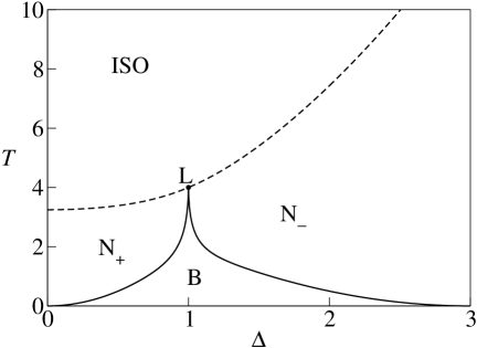
Figure 1: Phase diagram, in terms of temperature $T$ and the degree of biaxiality $\Delta$, for a system of intrinsically biaxial molecules. N₊ and N_- are uniaxial nematic prolate and oblate phases, respectively. B is the nematic biaxial phase, L is the Landau multicritical point, and ISO is the isotropic region. Continuous lines indicate continuous transitions and dashed lines represent first-order phase transitions.

Figure 1 shows the phase diagram in the $T-\Delta$ plane, which is obtained by solving the mean-field equations numerically. As it should be anticipated from phenomenological arguments, this phase diagram shows two lines of continuous transitions (solid lines) from a biaxial nematic region to the N₊ (prolate) and N_- (oblate) uniaxial nematic regions. These critical lines meet at a Landau multicritical point, L, on the first-order boundary (dashed lines) between the isotropic and the uniaxial nematic phases. It should be remarked that we regain an intrinsically uniaxial system for $\Delta=3$. The phase diagram for $\Delta>3$ is mapped onto the region $1<\Delta^{\prime}<3$ by the transformations $\Delta^{\prime}=\left(\Delta+3\right)/\left(\Delta-1\right)$ and $T^{\prime}=4T/\left(\Delta-1\right)^{2}$. Note that a similar model for asymmetric ellipsoids leads to essentially the same type of phase diagram Bocarra1970 . Also, a number of calculations for continuous orientational degrees of freedom lead to the same characteristic topology of this phase diagram (see, for example, the works of Luckhurst and collaborators Luckhurst2012 and of Xheng and Palffy-Murhoray Zheng2011 ).

From the expression of the free energy, we obtain the parameter-dependent coefficients of a Landau–de Gennes expansion about the Landau multicritical point,

$$A=1-\frac{3+\Delta^{2}}{T};\qquad B=\frac{9}{2}\left(\frac{\Delta^{2}-1}{T^{2}}\right);$$ (18)

$$C=\frac{1}{T^{3}}\left(\frac{9}{4}+\frac{3}{2}\Delta^{2}+\frac{1}{4}\Delta^{4}\right),$$ (19)

$$D=-\frac{45}{16T^{4}}\left(\Delta^{4}+2\Delta^{2}-3\right),$$ (20)

$$E=-\frac{1}{480T^{5}}\left(41\Delta^{6}+315\Delta^{4}+1215\Delta^{2}+1053\right),$$ (21)

$$E^{\prime}=\frac{1}{40T^{5}}\left(\Delta^{6}+225\Delta^{4}-405\Delta^{2}+243\right).$$ (22)

Therefore, the Landau point L is located at $T_{L}=4$ and $\Delta_{L}=1$. In the vicinity of L, limiting to first order terms in $\left(T-4\right)$ and $\left(\Delta-1\right)$, we have $A=\left(1/4\right)\left(T-4\right)-\left(1/2\right)(\Delta-1)$, $B=\left(9/16\right)\left(\Delta-1\right)$, $C=1/16$, $D=0$, $E=-41/7680$, and $E^{\prime}=1/640$. The sign of $E^{\prime}$ indicates the stability of the biaxial nematic phase near the Landau point deGennes ; Gramsbergen . In this mean-field scenario, at fixed $\Delta\neq 1$, as the temperature decreases from a sufficiently large value, the system goes from an isotropic phase to a uniaxial nematic phase, and then to a biaxial nematic phase, according to the prediction of the early work of Freiser Freiser . It should be remarked that the phenomenological Landau parameters are written in terms of the parameters of the underlying molecular model, which makes it easier to investigate a large range of values.

III.2 Annealed disorder

In the annealed case, we calculate $\psi$, given by Eq. (11), in terms of the proper thermodynamic field variables, temperature $T$ and chemical potential $\mu=\epsilon T\ln z$, where $z$ is a fugacity. For the fully-connected MS6 model of a binary mixture of uniaxial and biaxial molecules, the functional $\psi$ is given by

$$\psi=\frac{1}{2}\left(3S^{2}+\eta^{2}\right)-T\ln 2-T\ln\sigma,$$ (23)

where

$$\begin{split}\sigma&=e^{-\frac{3\left(S+\eta\right)}{2T}}\left\{1+z\cosh\left[\frac{\left(3S-\eta\right)\Delta}{2T}\right]\right\}\\ &\quad+e^{\frac{-3\left(S-\eta\right)}{2T}}\left\{1+z\cosh\left[\frac{\left(3S+\eta\right)\Delta}{2T}\right]\right\}\\ &\quad+e^{\frac{3S}{T}}\left\{1+z\cosh\left(\frac{\eta\Delta}{T}\right)\right\}\quad.\end{split}$$ (24)

Again, the thermodynamic stable values of $S$ and $\eta$ are chosen to minimize the function $\psi$ for fixed values of temperature $T$, degree of biaxiality $\Delta$, and chemical potential $\mu$.

Inserting the equilibrium values of $S$ and $\eta$ into the expression of $\psi$, we obtain the grand potential as a function of $T$, $\mu$, and $\Delta$. If we wish to work with a fixed concentration $c$ of the intrinsically biaxial molecules, the free energy $\phi\left(c,T;\Delta\right)$ comes from the definition

$$\phi\left(c,T;\Delta\right)=\psi+c\ln z,$$ (25)

where the fugacity is eliminated by the expression

$$c=-z\frac{\partial\psi}{\partial z},$$ (26)

and we should insert the equilibrium values of $S$ and $\eta$ (with the proviso of a Maxwell construction whenever it is necessary).

The grand potential can be used to write a Landau–de Gennes expansion with coefficients

$$A=1-\frac{3+z\left(3+\Delta^{2}\right)}{T\left(1+z\right)};\qquad B=\frac{9}{2}\frac{z\left(\Delta^{2}-1\right)-1}{T^{2}\left(1+z\right)};$$ (27)

$$C=\frac{9+z\left[18+9z+6(1+z)\Delta^{2}-(1-z)\Delta^{4}\right]}{4T^{3}\left(1+z\right)^{2}};$$ (28)

$$D=\frac{15}{16}\frac{9+z\left[18-6\Delta^{2}+\Delta^{4}-3z\left(-3+2\Delta^{2}+\Delta^{4}\right)\right]}{T^{4}\left(1+z\right)^{2}};$$ (29)

$$E=\frac{1053-z\left(c_{0}+zc_{1}+z^{2}c_{2}\right)}{480T^{5}\left(1+z\right)^{3}},$$ (30)

where

$$c_{0}=-3159-1215\Delta^{2}+225\Delta^{4}-11\Delta^{6},$$ (31)

$$c_{1}=-3159-2430\Delta^{2}-90\Delta^{4}+68\Delta^{6}$$ (32)

and

$$c_{2}=-1053-1215\Delta^{2}-315\Delta^{4}-41\Delta^{6},$$ (33)

$$E^{\prime}=\frac{243+z\left(d_{0}+zd_{1}\right)}{40T^{5}\left(1+z\right)^{2}},$$ (34)

where

$$d_{0}=486-405\Delta^{2}-45\Delta^{4}+\Delta^{6},$$ (35)

and

$$d_{1}=243-405\Delta^{2}+225\Delta^{4}+\Delta^{6}.$$ (36)

From the usual condition $A=B=0$, we locate a Landau multicritical point,

$$\mu_{L}=-T_{L}\ln\left(\Delta^{2}-1\right),\quad T_{L}=4,$$ (37)

which requires $\Delta^{2}>1$, and gives an indication of the existence of qualitatively different phase diagrams (as there is no Landau point for $\Delta^{2}<1$).

It is easy to show that this annealed version of the binary mixture exhibits phase diagrams with many distinct topologies. This can be anticipated from an analysis of the energy levels associated with the interaction between molecules, as shown in Figure 2. In fact, these energy levels are associated with different degrees of degeneracy $\omega$, and some levels cross each other as the biaxiality of the molecules is changed. These degeneracies account for entropic contributions to the free energy, which do affect the equilibrium phase behavior of the system. Therefore, we anticipate qualitative changes in the phase diagrams as $\Delta$ assumes values close to the location of the energy level crossings.

We now discuss the various topologies exhibited by the phase diagrams as the biaxiality parameter is changed.

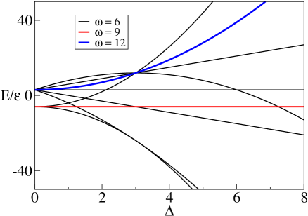
Figure 2: Energy levels as a function of the degree of biaxiality $\Delta$. Level crossings account for variations in the entropic contribution to the free energy.

Figures 3-4 show $T-\mu$ and $T-c$ phase diagrams for fixed degree of biaxiality, $\Delta=1$, where $\mu$ is the chemical potential and $c$ is the concentration of intrinsically biaxial molecules. From the thermodynamic point of view, the first-order boundaries (dashed lines) in the $T-\mu$ plane are mapped into coexistence regions (gray regions) in the $T-c$ plane. For low temperatures and intermediate concentrations, there is a coexistence region between the uniaxial prolate (N₊) and biaxial (B) phases. However, at higher concentrations and intermediate temperatures, there is a second-order phase transition (continuous line) between the N₊ and B phases. In fact, the phase diagram exhibits a tricritical point, TC, along the boundary between N₊ and B. At higher temperatures, there is a first-order phase transition between N₊ and the isotropic (ISO) phases, with a very thin coexistence region, as shown in the inset. Note that an incipient Landau point appears at $c=1$, which corresponds to an infinite chemical potential, in agreement with the Landau–de Gennes expansion. Phase diagrams with a similar topology (but with no Landau point) can be drawn for $0<\Delta<1$.

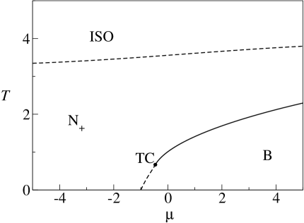
Figure 3: Phase diagram for fixed degree of biaxiality $\Delta=1$, where $T$ is temperature and $\mu$ is chemical potential. There is a tricritical point, TC, along the boundary separating biaxial (B) and uniaxial prolate nematic (N₊) phases. There is no direct phase transition between the isotropic (ISO) and biaxial phases (for finite values of the chemical potential).

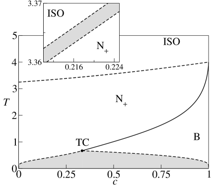
Figure 4: Phase diagram in terms of the temperature ($T$) versus the concentraton ($c$) of biaxial molecules, at a fixed degree of biaxiality, $\Delta=1$. There is an incipient Landau multicritical point at $c=1$, where the two ordered phases and the isotropic phase become identical. Uniaxial (N₊) and biaxial (B) phases coexist at low temperatures and intermediate concentrations (gray region). The system exhibits a tricritical point, TC, along the boundary of the B phase. The inset represents a zoom of the coexistence (gray) region between the uniaxial nematic and isotropic phases.

Figure 5 shows the phase diagram for a fixed degree of biaxiality $\Delta=1.4$. Similar to Figure 4, the N₊ and B phases coexist for intermediate concentrations and low temperatures. However, the system also displays a uniaxial oblate (N_-) nematic phase, which appears at higher concentrations and intermediate temperatures. The B phase appears between the two uniaxial phases, at intermediate temperatures. All three ordered phases become identical to the ISO phase at a Landau multicritical point, L. Also, note that the B phase presents a discrete reentrant behavior close to L. Note that the changes in the topology of the phase diagrams shown in Figures 4 and 5 are in agreement with the dependence of the energy levels on the degree of biaxiality $\Delta$ (see Figure 2).

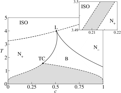
Figure 5: Phase diagram, in terms of temperature $T$ and concentration $c$ of biaxial molecules, for degree of biaxiality $\Delta=1.4$. There is a Landau point L. Note that the biaxial phase displays a reentrant behavior near L.

The phase behavior of the system changes significantly for degree of biaxiality around $\Delta=1.5$, which is close to another crossing of energy levels. For example, in Figure 6 we show the phase diagram for degree of biaxiality $\Delta=1.54$. The low temperature biaxial phase B_- is represented by a tensor order parameter $\mathbf{Q}$ whose largest eigenvalue (in absolute value) is negative. However, an additional biaxial phase B appears near the Landau point. The two biaxial phases are stable in disconnected regions of the phase diagram. There is then a coexistence region between the uniaxial nematic phases N₊ and N_-. This region is limited by two critical end points, CE, associated with the biaxial phases. Also, the system exhibits a tricritical point TC related to the coexistence region of N₊ and B structures. As in the case $\Delta=1.4$, shown in Figure 5, the biaxial phase is reentrant in the vicinity of the Landau point.

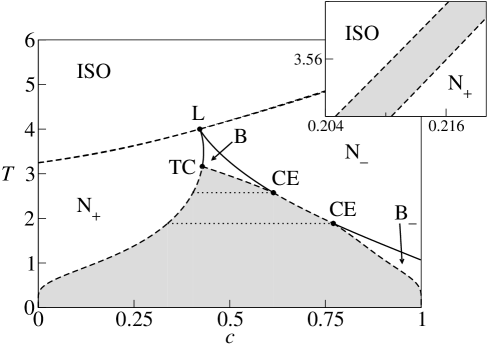
Figure 6: Phase diagram in the $c-T$ plane for degree of biaxiality $\Delta=1.54$, where $T$ is the temperature and $c$ is the concentation of biaxial objects. Two nematic biaxial phases are stable in disconnected regions of the phase diagram. There is a coexistence region between the nematic uniaxial phases, ending at two critical end points CE. The dotted horizontal lines represent special tie lines associated with the critical end points.

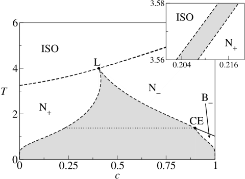
Figure 7: Phase diagram in terms of temperature ($T$) versus concentrarion ($c$) of biaxial molecules for fixed degree of biaxiality, $\Delta=1.57$. The biaxial phase B_- is located at low temperatures and high concentations. There is no stable B phase near the Landau point L. The nematic uniaxial phases coexist in a region ending at a critical end point CE. The dotted horizontal line represents a special tie line associated with the critical end point.

The topological changes in the phase diagram can be represented by the projections of the lines of different multicritical points on the $T-\Delta$ plane, as indicated in Figure 8. The temperature of the Landau point (black) is a constant function of the degree of biaxiality $\Delta$, which is in agreement with a Landau expansion. The temperature of the tricritical point (green) increases monotonically with $\Delta$, as suggested by Figures 4-6. However, the line of critical end points (blue) presents a reentrant behavior in the vicinity of $\Delta=1.55$, giving rise to the two critical end points, as it is shown in Figure 6. All multicritical lines meet at a higher-order multicritical point M₁. Note that the tricritical and high-temperature critical end points are associated with the biaxial phase near the Landau point. As a result, there is no stable biaxial phase in the vicinity of L for $\Delta\geq\Delta_{M_{1}}\simeq 1.5576$, although the low-temperature biaxial phase survives in a small region at high concentrations and low temperatures. This is illustrated in Figure 7, for $\Delta=1.57$. There is no stable biaxial nematic phase close to the Landau point L, which marks the meeting of various coexistence lines separating the isotropic phase and the two nematic uniaxial phases. Along those lines, there is a coexistence of phases with different values of nematic order parameter $S$, but the size of the coexistence region tends to vanish as we approach the Landau point.

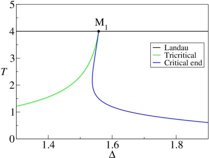
Figure 8: Lines of multicritical points in the $\Delta-T$ plane. There is a higher-order multicritical point M₁, at which the lines of Landau points (black), tricritical points (green) and critical end points (blue) meet. There is then no stable biaxial phase for $\Delta\geq\Delta_{\text{M}_{1}}$ in the vicinity of the Landau point.

As the degree of biaxiality is further increased, the system exhibits other distinct phase diagrams, as seen in Figures 9-10. According to Figure 2, multiple level crossings occur at $\Delta=3$, which is a strong suggestion of changes in the phase behavior of the system.

Figure 9 shows the phase diagram for $\Delta=2.9$. There appears a triple point associated with the coexistence of two uniaxial nematic oblate phases and a uniaxial prolate phase. Also, the coexistence region of uniaxial nematic oblate phases ends at a simple critical point C. Although it is not shown in Figure 9, a stable biaxial nematic phase is still present, at low temperatures and high concentrations, as well as the critical end point associated with the biaxial phase.

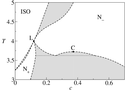
Figure 9: Phase diagram in terms of temperature $T$ and concentration $c$ of biaxial objects, for degree of biaxiality $\Delta=2.9$. There is no biaxial nematic phase around the Landau point L. C indicates a simple critical point associated with a coexistence region between two uniaxial oblate phases. The dotted line indicates a triple point, corresponding to the coexistence of two uniaxial oblate and one uniaxial prolate phases.

As $\Delta$ is further increased, the simple critical point moves upward in the phase diagram, approaching the lower border of the coexistence region between the uniaxial $\mathrm{N}_{-}$ and ISO phases. Then, the simple critical point is replaced by a second triple point. For example, Figure 10 represents a phase diagram for $\Delta=3$. Due to the second triple point, there appears an isolated second uniaxial oblate phase $\mathrm{N}_{-}^{(2)}$. Note that, according to Eq.(II), the value $\Delta=3$ corresponds to a binary mixture of rods and plates with asymmetric interaction energies. A symmetric choice of interaction energies ECarmo2011 presents a much simpler phase diagram, with single nematic uniaxial prolate and oblate phases, in addition to an isotropic phase, and no triple points.

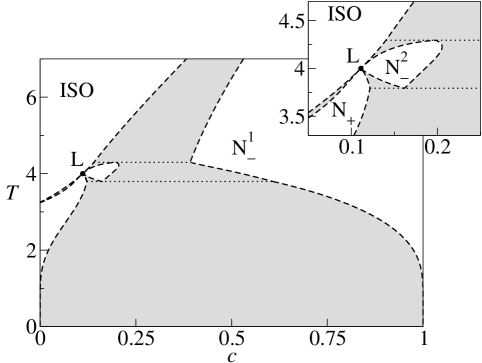
Figure 10: Phase diagram in terms of temperature $T$ and concentration $c$ of biaxial objects, for degree of biaxiality $\Delta=3.0$. This system corresponds to a mixture of rods and plates with asymmetric interaction energies. A uniaxial nematic prolate phase, $\mathrm{N}_{+}$, and two uniaxial nematic oblate phases, $\mathrm{N}_{-}^{1}$ and $\mathrm{N}_{-}^{2}$, are present. There are two triple points indicated by the dotted tie lines.

Figures 11 and 12 represent the phase diagrams for $\Delta=5$ and $\Delta=6$, respectively. In these diagrams the values of concentrations are conveniently rescaled, so that visual effects are improved. Also, note that we introduce some separations just to emphasize the more interesting sectors of this phase diagram. There is no stable Landau point in both phase diagrams. In Figure 11, the uniaxial phases N₊ and N_- coexist with the ISO phase at a triple point, and a biaxial B_- phase remains stable at high concentrations. However, in Figure 12, there is a coexistence region of B_- and ISO phases, as well as a triple point of coexistence of ISO, B_- and N₊ phases. Figures 11 and 12 suggest that the triple points meet the critical end point as the degree of biaxiality is increased.

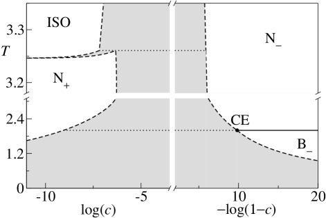
Figure 11: Phase diagram in terms of temperature $T$ and concentration $c$ of biaxial molecules, for degree of biaxiality $\Delta=5.0$. The Landau point is absent. There appears a triple point, at which N₊, N_- and ISO phases coexist. The B_- phase is stable at high concentations.

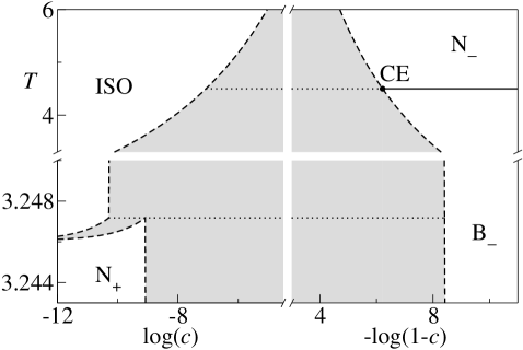
Figure 12: Phase diagram in terms of temperature $T$ and concentration $c$ of biaxial objects, for degree of biaxiality $\Delta=6.0$. The Landau point is absent. There is a coexistence region between ISO and B_- phases. In addition, ISO, B_- and N₊ phases coexist at a triple point. The B_- phase is stable at high concentations.

In Figure 13 we draw the projections of distinct multicritical points on the $\Delta-T$ plane. The line of Landau points is still present, as well as the low-temperature part of the line of critical end points associated with B_-. Furthermore, there are lines of triple points associated with the ISO and various nematic uniaxial phases, as depicted in Figures 9 and 10. The line of Landau points meets the triple lines at another special multicritical point, which we call a Landau end point, LE. This point is characterized by the coexistence of a critical ISO phase and a non-critical N_- phase. Otherwise, two triple lines meet the line of simple critical points at two multicritical end points, MCE. In addition, for $\Delta\simeq 5.5$, the triple line meets the critical end line at a multicritical point, M₂, where the critical phase N_- coexists with the non-critical phases N₊ and ISO. Consequently, for $\Delta\geq 5.5$, there is a coexistence region between ISO and B_- phases as we increase the concentration of biaxial molecules.

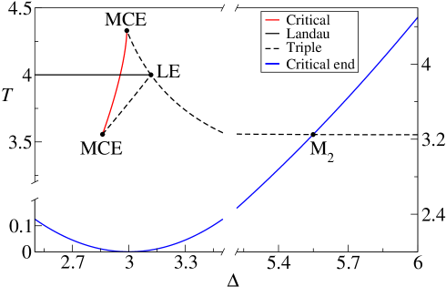
Figure 13: Lines of phase transitions in the $\Delta-T$ plane. The dashed black lines represent lines of triple points. The line of simple critical points (red) ends at two multicritical end points MCE. The line of Landau poins meets the lines of triple points at a Landau end point LE. Also, the line of critical end points (blue) crosses the line of triples points at a multicritical point M₂.

IV Conclusions

We introduced an elementary six-state Maier-Saupe (MS6) lattice model, which is obtained by the addition of extra degrees of freedom, of biaxial nature, to an earlier three-state model. We then described a phase diagram with biaxial as well uniaxial nematic structures and an isotropic phase. A fully connected MS6 lattice model, of mean-field character, is sufficiently simple to be amenable to a detailed treatment by standard statistical mechanics techniques. Results are obtained in terms of a parameter $\Delta$ of shape fluctuations that gauges the degree of biaxiality. We then used this MS6 model to consider a binary mixture of intrinsically uniaxial ($\Delta=0$) and intrinsically biaxial ($\Delta\neq 0$) molecules, and investigated the effects of “shape fluctuations" on the phase diagrams in terms of temperature and either chemical potential or concentration of biaxial molecules.

Taking into account the fluid character of the liquid-crystalline systems, in the present work we restricted the analysis to a thermalized (annealed) situation, in which case orientational and shape degrees of freedom reach equilibrium simultaneously. We obtained a wealth of topologically distinct phase diagrams, with several nematically ordered structures and multicritical points.

In the uniform case, in terms of temperature $T$ and the parameter $\Delta$, we regained the first-order transitions between isotropic and uniaxial nematic phases, and the critical lines between the biaxial and uniaxial nematic phases, which meet at a Landau multicritical point. For a binary mixture of biaxial and uniaxial molecules, we have drawn a number of phase diagrams in terms of temperature versus concentration of biaxial molecules, with fixed values of $\Delta$, which display many distinct features. Depending on parameters, there appear additional multicritical points, such as tricritical and critical end points associated with the biaxial nematic phase. The Landau, tricritical and critical end points may give rise to a higher-order multicritical point. Also, depending on the range of values of $\Delta$, there may be a line of Landau points meeting a line of triple points at a Landau end point. This intricate behavior of the mixtures of intrinsically uniaxial and biaxial molecules can be understood in terms of crossings of the microscopic energy levels as we change the degree of biaxiality $\Delta$.

The explicit expressions for the free energy were used to obtain the coefficients of an expansion at high temperatures, in the vicinity of the Landau multicritical point, and to make contact with the Landau-de Gennes theory. We were then able to check our numerical findings against a number of phenomenological calculations of the literature. Also, we provided a simple way of obtaining the expansion coefficients in terms of the values of the molecular parameters.

The calculations predict the presence of stable biaxial nematic phase at low temperatures and sufficiently high concentrations of biaxial molecules, which is in agreement with recent calculations of Longa and coworkers LongaPajakWydro for a more elaborate model system of a mixture of biaxial molecules in the annealed situation. Depending on the degree of biaxiality, we predict first-order transitions between biaxial and uniaxial nematic phases, as well as tricritical points, even in the absence of a Landau multicritical point. For larger values of the degree of biaxiality, the Landau point splits into lines of triple points. Also, we note a clear reentrance of the biaxial regions for some choices of the parameters, which is agreement with the early work of Alben for a lattice model of platelets Alben .

In some recent publications, Akpinar, Reis, and Figueiredo-Neto AkpinarEPJE AkpinarLC reported X-ray and optical characterizations of biaxial nematic structures in a large class of quaternary liquid-crystalline mixtures. From these measurements, it has been possible to establish many novel phase diagrams in terms of temperature and molar fraction of the components, which represents a real advance with respect to the early work of Yu and Saupe for a ternary lyotropic mixture. For all concentrations of the amphiphile component, if there is a nematic biaxial structure, it is thermodynamically stable at intermediate temperatures, between regions of different uniaxial nematic structures, at lower and higher temperatures. Also there are examples of temperature-concentration phase diagrams with a clear indication of the existence of a Landau multicritical point. With a suitable choice of parameters, the MS6 model of a binary mixtures can qualitatively reproduce all of these observations. In a very recent experimental investigation, Amaral and coworkers Amaral reanalyzed the phase diagram of a ternary SDS lyotropic mixture, and pointed out a peculiar coexistence of uniaxial and biaxial nematic structures, which still seems to demand a theoretical explanation.

The present calculations, for the elementary MS6 lattice model, at the mean-field level, are a contribution to the understanding of the effects of shape fluctuations on the thermodynamic behavior of complex liquid-crystalline systems. The model of a binary mixture is sufficiently simple to produce a number of analytical and numerical results for a wide range of values of the molecular parameters. Also, it seems to be possible to go beyond the mean-field scenario. The use of more powerful techniques may uncover additional aspects of the phase diagrams, in particular limitations of the mean-field approach at very low and very high concentrations.

- (1) B. R. Acharya, A. Primak, and S. Kumar, Phys. Rev. Lett. 92, 145506 (2004).
- (2) L. A. Madsen, T. J. Dingemans, M. Nakata, and E. T. Samulski, Phys. Rev. Lett. 92, 145505 (2004).
- (3) K. Merkel, A. Kocot, J. K. Vij, R. Korlacki, G. H. Mehl, and T. Meyer, Phys. Rev. Lett. 93, 237801 (2004).
- (4) G. R. Luckhurst, Nature 430, 413 (2004).
- (5) M. J. Freiser, Phys. Rev. Lett. 24, 1041 (1970).
- (6) R. Alben, Phys. Rev. Lett. 30, 778 (1973).
- (7) N. Bocarra, R. Medjani, and L. de Sèze, J. Phys. 38, 149 (1970).
- (8) J. P. Straley, Phys. Rev. A10, 1881 (1974).
- (9) G. R. Luckhurst, S. Naemura, T. J. Sluckin, K. S. Thomas and S. S. Turzi, Phys Rev E, 85, 031705 (2012).
- (10) L. J. Yu and A. Saupe, Phys. Rev. Lett. 45, 1000 (1980).
- (11) R. Berardi, L. Muccioli, S. Orlandi, M. Ricci, and C. Zannoni, J. Phys.: Cond. Matter 20, 463101 (2008).
- (12) Y. Martinez-Ratón and J. A. Cuesta, Phys. Rev. Lett. 89, 185701 (2002).
- (13) E. F. Henriques and V. B. Henriques, J. Chem. Phys. 107, 8036 (1997).
- (14) E. do Carmo, D. B. Liarte, and S. R. Salinas, Phys. Rev. E81, 062701 (2010).
- (15) E. do Carmo, A. P. Vieira, and S. R. Salinas, Phys. Rev. E 83, 011701 (2011).
- (16) L. Longa, G. Pajak, and T. Wydro, Phys Rev E76, 011703 (2007).
- (17) M. J. de Oliveira and A. M. Figueiredo Neto, Phys. Rev. A34, 3481 (1986).
- (18) S. K. Ma, Modern Theory of Critical Phenomena, W. Benjamin, New York, 1976.
- (19) P. G. de Gennes and J. Prost, The Physics of Liquid Crystals, Oxford University Press, New York, 1993.
- (20) Thomas A. Witten and Philip Pincus, Structural Fluids: Polymers, Colloids, Surfactants, Oxford University Press, New York, 2004, Chapter 2.
- (21) E. F. Gramsbergen, L. Longa, and W. H. de Jeu, Physics Reports 135, 195 (1986).
- (22) X. Zheng and P. Palffy-Murhoray, Discrete and Continuous Dynamical Systems B 15, 475 (2011).
- (23) E. Akpinar, D. Reis, and A. M. Figueiredo Neto, Eur. Phys. J. E 35, 50 (2012).
- (24) E. Akpinar, D. Reis, and A. M. Figueiredo Neto, Liquid Crystals 39, 881 (2012).
- (25) L. Q. Amaral, O. R. Santos, W. S. Braga, N. M. Kimura, and A. J. Palangana, Liquid Crystals 42, 240 (2015).