Perturbative entanglement thermodynamics

for AdS spacetime: Renormalization

Rohit Mishra and Harvendra Singh

Theory Division, Saha Institute of Nuclear Physics

1/AF Bidhannagar, Kolkata 700064, India

Abstract

We study the effect of charged excitations in the AdS spacetime on the first law of entanglement thermodynamics. It is found that ‘boosted’ AdS black holes give rise to a more general form of first law which includes chemical potential and charge density. To obtain this result we have to resort to a second order perturbative calculation of entanglement entropy for small size subsystems. At first order the form of entanglement law remains unchanged even in the presence of charged excitations. But the thermodynamic quantities have to be appropriately ‘renormalized’ at the second order due to the corrections. We work in the perturbative regime where $T_{thermal}\ll T_{E}$.

1 Introduction

The AdS/CFT correspondence [1] has been a very successful idea in string theory. It relates conformal field theries living on the boundary of anti de Sitter (AdS) spacetime with the supergravity theory in the bulk. The idea of entanglement entropy has also been a focus of recent study in string theory [2]. It has led to some understanding of entanglement entropy in strongly coupled quantum mechanical systems, particularly theories which exhibit scaling property near the critical points [3]. A significant observation has been that the small excitations of the subsystems in the boundary theories follow entanglement thermodynamic laws similar to the black hole thermodynamics at finite temperature [4, 5, 6]. These calculations have become possible now because entanglement entropy can be estimated using the gauge/gravity holography [2], that is by evaluating the geometrical area of extremal sufaces embedded inside the bulk (AdS) geometry. It has been proposed recently in [4] that the entanglement entropy ($S_{E}$) and the energy of excitations (${\cal E}$) in pure AdS background give rise to a relation

$$\bigtriangleup{\cal E}=T_{E}\bigtriangleup S_{E}+\cdots$$

which has been described as the first law of entanglement thermodynamics [4].

In this paper we study the effects of IR deformations (excitations) in asymptotically AdS spacetime which carry gauge charges and look for modifications in the entanglement first law. We do find that the ‘boosted’ AdS black holes give rise to a more general form of first law which includes the chemical potential and charge density. To obtain this result we have to resort to a second order perturbative calculation of the entanglement entropy. We find that various first order thermodynamic quantities, such as entropy, energy, temperature, etc get corrected and these have to be suitably redefined or ‘renormalized’ at the second order. The effects of higher order corrections appears similar to the renormalization procedure in quantum field theories. For example the strip width (subsystem size) and entanglement temperature ($T_{E}$) have to be redefined to include corrections so that a first law like relation holds good. Since we resort to perturbative calculations, we work in the regime where the ratio ${l\over z_{0}}$, of the strip width ($l$) to the horizon radius ($z_{0}$), is kept very small. This hierarchy of scales can also be thought of in terms of respective temperatures as a limit

$${T_{thermal}\over T_{E}}\ll{a_{1}\over 2b_{0}\gamma}\ .$$

We mention that the corrections to the entanglement entropy evaluated order by order in (dimensionless) quantity ${T_{thermal}\over T_{E}}$ should not be confused with (stringy) quantum corrections to the entanglement entropy [9].

The paper is organised as follows. In the section-2 we mainly work out the first law of entanglement thermodynamics for AdS black holes in presence of boost. We get the familiar form of the law which has the same temperature as in the unboosted case, eventhough the charged excitations are present, while the energy of excitations increases compared to the unboosted case. We work out the entanglement entropy up to second order in section-3. It is found that the form of first law changes under these corrections. The chemical potential explicitly appears in the first law at the second order. The temperature and other thermodynamic quantities need to be renormalized. In fact the entanglement temperature slightly decreases with corrections. The conclusions are given in the section-4.

2 Entanglement from boosted AdS black holes

The boosted $AdS_{d+1}$ black holes backgrounds are given by

$$ds^{2}={L^{2}\over z^{2}}\left(-{fdt^{2}\over K}+K(dy-\omega)^{2}+dx_{1}^{2}+\cdots+dx_{d-2}^{2}+{dz^{2}\over f}\right)$$ (1)

with

$$f=1-{z^{d}\over z_{0}^{d}},~{}~{}~{}~{}~{}K=1+\beta^{2}\gamma^{2}{z^{d}\over z_{0}^{d}}$$ (2)

$z_{0}$ is the horizon and $0\leq\beta\leq 1$ is boost parameter, while $\gamma={1\over\sqrt{1-\beta^{2}}}$. The boost is taken along $y$ direction. The Kaluza-Klein form

$$\omega={\beta^{-1}}(1-{1\over K})dt$$ (3)

and $L$ is the radius of curvature of AdS spacetime, which is very large.

We study the entanglement entropy of a subsystem on the boundary of boosted $AdS_{d+1}$ backgrounds in (1). We embed a $(d-1)$-dimensional strip-like spatial surface, in the bulk asymptotic geometry. The boundaries of the extremal bulk surface coincide with the two ends of the interval $-l/2\leq x^{1}\leq l/2$. The regulated size of the rest of the coordinates is taken large $0\leq x^{i}\leq l_{i}$, with $l_{i}\gg l$. We shall always have coordinate $y$ being compact, so that $0\leq y\leq 2\pi r_{y}$. As per the Ryu-Takayanagi prescription [2] the entanglement entropy is given in terms of the geometrical area of the extremal surface

$$S_{E} \equiv {[A]_{Strip}\over 4G_{d+1}}$$ (4)

$$= {V_{d-2}L^{d-1}\over 2G_{d+1}}\int^{z_{\ast}}_{\epsilon}{dz\over z^{d-1}}\sqrt{K}\sqrt{{1\over{f}}+({\partial_{z}x^{1}})^{2}}$$

where $G_{d+1}$ is $(d+1)$-dimensional Newton’s constant and $V_{d-2}\equiv(2\pi r_{y})l_{2}l_{3}\cdots l_{d-2}$ is the spatial volume of the boundary. We will be mainly working for $d>2$. In our notation $\epsilon\sim 0$ denotes the cut-off scale near the boundary to regularize the UV divergences, and $z_{\ast}$ is the turning point of extremal surface inside the bulk geometry. In the above $K(z),~{}f(z)$ are known functions, so we only need to solve for $x^{1}$. From (4) it follows that a minimal surface will have to satisfy

$${dx^{1}\over dz}\equiv{({z\over z_{c}})^{d-1}}{1\over\sqrt{f}\sqrt{K-({z\over z_{c}})^{2d-2}}}$$ (5)

The constant $z_{c}$ is given by the turning point relation

$${K_{\ast}}-({z_{\ast}\over z_{c}})^{2d-2}=0$$ (6)

where $K_{\ast}=K(z)|_{z=z_{\ast}}$. The identification of the boundary $x^{1}(0)=l/2$ leads to the integral relation

$${l\over 2}=\int_{0}^{z_{\ast}}dz({z\over z_{\ast}})^{d-1}{1\over\sqrt{f}\sqrt{{K\over K_{\ast}}-({z\over z_{\ast}})^{2d-2}}}$$ (7)

which relates $l$ with $z_{\ast}$, the turning point. The turning-point takes the mid-point value $x^{1}(z_{\ast})=0$ on the boundary. The expression of the entanglement entropy for these boosted AdS black hole solutions becomes

$$S_{E}={V_{d-2}L^{d-1}\over 2G_{d+1}}\int^{z_{\ast}}_{\epsilon}{dz\over z^{d-1}}{K\over\sqrt{f}\sqrt{K-K_{\ast}({z\over z_{\ast}})^{2d-2}}}$$ (8)

The expression (8) mathematically provides the entanglement entropy for a strip-like subsystem on the boundary. For pure AdS spacetime ($z_{0}\to\infty,~{}f=1=K$) these integrals can be evaluated exactly [2], but in the presence of black hole it is difficult to find analytical answers from the integral (8), although numerical estimates can always be made.

2.1 Thin strip approximation

In the cases where the strip subsystem is a small part of a big system, so that the turning point lies in the proximity of asymptotic boundary region only ($z_{\ast}\ll z_{0}$), one can evaluate the entanglement entropy integral (8) by expanding it around its pure AdS value (treating pure AdS as a ground state). We shall take boost to be finite but small $\beta\gamma\sim 1$. Under these approximations the strip width equation (7) can be expanded perturbatively as

$${l} = 2\int_{0}^{z_{\ast}}dz({z\over z_{\ast}})^{d-1}{1\over\sqrt{f}\sqrt{{K\over K_{\ast}}-({z\over z_{\ast}})^{2d-2}}}$$ (9)

$$=2z_{\ast}\int_{0}^{1}d\xi\xi^{d-1}{1\over\sqrt{R}}[1+{1\over 2}{z_{\ast}^{d}\over z_{0}^{d}}\xi^{d}+{\beta^{2}\gamma^{2}z_{\ast}^{d}\over 2z_{0}^{d}}{1-\xi^{d}\over R}+\cdots]$$

$$\equiv 2z_{\ast}\left(b_{0}+{z_{\ast}^{d}\over 2z_{0}^{d}}(b_{1}+\beta^{2}\gamma^{2}I_{l})\right)+\cdots$$

where we have introduced $\xi={z\over z_{\ast}}$, $R\equiv 1-\xi^{2d-2}$ and the dots indicate terms of higher order in $({z_{\ast}\over z_{0}})^{d}$. The coefficients $b_{0},b_{1}$, and $I_{l}$ are precise integral Beta functions multiplying at various orders. These coefficients are provided in the appendix. Note $b_{0}$ and $b_{1}$ are positive definite quantities. Keeping only up to first order in $(z_{\ast}^{d}/z_{0}^{d})$ the equation (9) can be inverted to obtain

$$z_{\ast} = {l/2\over b_{0}+{z_{\ast}^{d}\over 2z_{0}^{d}}(b_{1}+\beta^{2}\gamma^{2}I_{l})}\simeq{\bar{z}_{\ast}\over 1+{\bar{z}_{\ast}^{d}\over 2z_{0}^{d}}({b_{1}\over b_{0}}+{\beta^{2}\gamma^{2}\over b_{0}}I_{l})}$$ (10)

where $\bar{z}_{\ast}\equiv{l\over 2b_{0}}$ being the turning point value in pure AdS case having the same strip width $l$. The last equation summarizes geometrically the whole effect of IR bulk deformations (excitations), like having ‘black hole in geometry’ and boosts on the turning point value, perturbatively.

Having obtained the turning point expansion, a similar expansion around pure AdS can be made for the area functional also. After regularizing the area integral (8), in the UV limit $(\epsilon\to 0)$, we find the following expansion

$$A \equiv 2\int_{0}^{z_{\ast}}{dz\over z^{d-1}}{K\over\sqrt{f}\sqrt{K-K_{\ast}({z\over z_{\ast}})^{2d-2}}}+A_{UV}$$ (11)

$$= 2\int_{0}^{z_{\ast}}{dz\over z^{d-1}}{1\over\sqrt{R}}[1+{1+\beta^{2}\gamma^{2}\over 2}{z^{d}\over z_{0}^{d}}+{\beta^{2}\gamma^{2}\over 2}{(z_{\ast}^{d}-z^{d})\over z_{0}^{d}}(-1+{1\over R})+\cdots]+A_{UV}$$

where we have denoted diverging UV part as $A_{UV}={2\over d-2}{1\over\epsilon^{d-2}}$. The respective finite integrals can be evaluated at each order on the right hand side to give

$$A = {2\over z_{\ast}^{d-2}}[a_{0}+{z_{\ast}^{d}\over 2z_{0}^{d}}(\gamma^{2}a_{1}+\beta^{2}\gamma^{2}I_{l})+\cdots]+A_{UV}$$ (12)

$$={2a_{0}\over z_{\ast}^{d-2}}[1+{z_{\ast}^{d}\over 2z_{0}^{d}}(\gamma^{2}{a_{1}\over a_{0}}+{\beta^{2}\gamma^{2}\over a_{0}}I_{l})+\cdots]+A_{UV}$$

where new coefficients $a_{0},a_{1},...$ are specific Beta-function integrals given in the appendix. We should note that $a_{1}>0$, but using Beta function identities we shall have $a_{0}=-{b_{0}\over d-2}$, so $a_{0}$ will be negative for all $d>2$. Now substituting for $z_{\ast}$ from (10) and only keeping terms up to first order we find that

$$A =A_{UV}+{2a_{0}\over\bar{z}_{\ast}^{d-2}}\left(1+{\bar{z}_{\ast}^{d}\over z_{0}^{d}}{d-2\over 2}({b_{1}\over b_{0}}+\beta^{2}\gamma^{2}{I_{l}\over b_{0}})+{\bar{z}_{\ast}^{d}\over 2z_{0}^{d}}(\gamma^{2}{a_{1}\over a_{0}}+{\beta^{2}\gamma^{2}}{I_{l}\over a_{0}})\right)$$ (13)

$$=A_{UV}+A_{0}\left(1+{\bar{z}_{\ast}^{d}\over z_{0}^{d}}{d-2\over 2}{b_{1}\over b_{0}}+{\bar{z}_{\ast}^{d}\over 2z_{0}^{d}}\gamma^{2}{a_{1}\over a_{0}}\right)$$

$$\equiv A_{UV}+A_{0}+A_{1}$$

where in the second last line the terms involving $I_{l}$ have got exactly cancelled! We have defined

$$A_{0}={2a_{0}\over\bar{z}_{\ast}^{d-2}}=-{(2b_{0})^{d-1}\over(d-2)l^{d-2}}$$ (14)

as the area contribution for pure $AdS_{d+1}$ with turning point $\bar{z}_{\ast}$ and strip width $l$. The term $A_{1}$ contains all the first order contributions to the area. As a check, for pure AdS ( $A_{1}=0$) we get the standard result [2]

$$A_{AdS}={1\over d-2}\left({2\over\epsilon^{d-2}}-{2^{d-1}b_{0}^{d-1}\over l^{d-2}}\right).$$ (15)

which is a positive definite quantity. From equation (13) we also find the net change in the area of extremal surface due to IR deformations (black hole with boost). It is given by

$$\bigtriangleup A\equiv A-A_{AdS} = {a_{0}\bar{z}_{\ast}^{2}\over z_{0}^{d}}\left((d-2){b_{1}\over b_{0}}+\gamma^{2}{a_{1}\over a_{0}}\right)$$ (16)

$$={a_{1}l^{2}\over 4b_{0}^{2}}\left({d-1\over d+1}+\beta^{2}\gamma^{2}\right){1\over z_{0}^{d}}$$

where in the second line we have used the relation between two ratios ${b_{1}\over b_{0}}=-{2\over(d+1)(d-2)}{a_{1}\over a_{0}}$. It is remarkable to note that the remainder of the expression on the right hand side of eq.(16) is positive definite, which suggests that the net area of the extremal strip has effectively increased as compared to the pure AdS. The presence of $\beta$ dependent terms precisely contain the effect of boost on the area of the extremal surface. In the absence of boost these terms will be absent and we shall get the result first obtained by [4]. It suggests that the boosting of the bulk metric (which forms a type of charged excitations in the CFT_d) increases the strip area and hence increases the entanglement entropy for the CFT subsystem. Following from (16) the change in entanglement entropy above the pure AdS ground state, up to first order is given by

$$\bigtriangleup S={L^{d-1}V_{d-2}\over 16G_{d+1}}{a_{1}l^{2}\over b_{0}^{2}}\left({d-1\over d+1}+\beta^{2}\gamma^{2}\right){1\over z_{0}^{d}}\ .$$ (17)

The equation (17) is an important expression for the remaining part of the analysis in this section.

2.2 Entanglement First Law

It is left now to carefully partition the right hand side in terms of physical thermodynamic observables of the CFT. The physical quantities such as energy, charge and pressure can be obtained by expanding the bulk geometry (1) in suitable Fefferman-Graham (asymptotic) coordinates near the AdS boundary [8], given in the appendix. These for the subsystem of CFT_d (on a circle) are summarised here. The energy and charge for the strip subsystem are

$$\bigtriangleup{\cal E}={dL^{d-1}V_{d-2}l\over 16\pi G_{d+1}}<t_{00}>={r_{y}L^{d-1}V_{d-3}l\over 8G_{d+1}}({d-1\over d}+\beta^{2}\gamma^{2}){d\over z_{0}^{d}}$$

$$\bigtriangleup{\cal N}\equiv r_{y}P_{y}={r_{y}L^{d-1}V_{d-2}l\over 16\pi G_{d+1}}{\beta\gamma^{2}d\over z_{0}^{d}}$$ (18)

respectively. The pressure component along the $x_{1}$ direction of the compactified CFT is

$$\bigtriangleup{\cal P}={2\pi r_{y}L^{d-1}d\over 16\pi G_{d+1}}<t_{11}>={L^{d-1}r_{y}\over 8G_{d+1}}{1\over z_{0}^{d}}$$ (19)

while $V_{d-3}\equiv l_{2}l_{3}\cdots l_{d-2}$, and $d$-dimensional Newton’s constant ${1\over G_{d}}={2\pi r_{y}L\over G_{d+1}}$. The ${\cal{N}}$ represents integral value of (momentum) charge. In the absence of boost it would be vanishing. We note down nontrivial chemical potential in our solutions. It is given by the value of gauge potential $\omega$ at the turning point,

$$\mu={1\over r_{y}\beta}(1-{1\over K(z_{\ast})})\simeq{\beta\gamma^{2}\over r_{y}}{\bar{z}_{\ast}^{d}\over z_{0}^{d}}$$ (20)

Hence the contribution of ‘entanglement chemical potential’ would remain negligible in first order of approximation we are working in this section. (Note, the corresponding thermal value of chemical potential is however large $\mu_{{}_{thermal}}={\beta\over r_{y}}$.)

Our aim is to express the right hand side of (17) in terms of above physical observables. From (2.2), a little guess tells us that

$$\left({d-1\over d+1}+\beta^{2}\gamma^{2}\right){1\over z_{0}^{d}}\equiv\bigg{[}({d-1\over d}+\beta^{2}\gamma^{2})-{d-1\over d+1}{1\over d}\bigg{]}{1\over z_{0}^{d}}$$ (21)

Using (2.2) and (19) we can now express eq.(17) as

$$\bigtriangleup S_{E}={1\over T_{E}}\left(\bigtriangleup{\cal E}-{d-1\over d+1}~{}{\cal V}\bigtriangleup{\cal P}\right)$$ (22)

where ${\cal V}\equiv l[V_{d-3}]$ is the net volume of the subsystem. The equation (22) simply describes the first law of entanglement thermodynamics, which is identical to the result in [5]. An alternative first law form was first proposed by [4] for the isotropic AdS case. It leads to a difference in entanglement temperatures. If we set $\beta=0$ in (22), it reduces to the known first law form obtained in [5]. Hence we can conclude that the form of the first law remains true for ‘boosted’ AdS black-hole case as well, eventhough the excitations in CFT are much different in the boosted case. For example, there are quantized charges present in these backgrounds. The entanglement temperature is given as

$$T_{E}={b_{0}^{2}\over a_{1}}{d\over\pi l}={(B({d\over 2d-2},{1\over 2}))^{2}\over 2(d-1)B({1\over d-1},{1\over 2})}{d\over\pi l}.$$ (23)

The temperature is inversely proportional to the width of strip. But this temperature is lower by a factor ${d\over d+1}$ as compared to the isotropic case in [4]. It is evident that there is no explicit charge dependence in the first law equation (22). The reason for this is that the entanglement chemical potential given in (20) remains negligible $(\sim O(z_{\ast}^{d}/z_{0}^{d}))$ at the first order. The contribution of chemical potential will however become important in next higher order calculation which we perform in the following section. This contribution is expected to change the ‘first order’ form of the first law (22).

3 Entanglement entropy at second order

Taking similar steps as in the previous section, we now calculate the second order terms in the expansion of the area integral schematically denoted as

$$A\equiv A_{UV}+A_{0}+A_{1}+A_{2}$$ (24)

where $A_{0}$ and all first order terms contributing to $A_{1}$ have been obtained in the previous section. Our aim is to find $A_{2}$. First, we obtain the expansion of the turning point value, as done in (10), up to second order

$$z_{\ast} = \bar{z}_{\ast}\left(1+{\bar{z}_{\ast}^{d}\over z_{0}^{d}}({b_{1}+\beta^{2}\gamma^{2}I_{l}\over 2b_{0}})+{\bar{z}_{\ast}^{2d}\over z_{0}^{2d}}\left({\bar{b}_{2}+J_{l}\over b_{0}}-d({b_{1}+\beta^{2}\gamma^{2}I_{l}\over 2b_{0}})^{2}\right)\right)^{-1}$$ (25)

where $\bar{b}_{2}\equiv{3\over 8}b_{2}$. The coefficients $b_{2},~{}I_{l},~{}J_{l}$ are given in the appendix. There is no need to simplify this expression further at this step. A lengthy calculation leads to following second order contribution

$$A_{2}={2a_{0}\over\bar{z}_{\ast}^{d-2}}\bigg{[}(d+3){(b_{1}+\beta^{2}\gamma^{2}I_{l})^{2}\over 8a_{0}b_{0}}-{(b_{1}+\beta^{2}\gamma^{2}I_{l})(\gamma^{2}a_{1}+\beta^{2}\gamma^{2}I_{l})\over 2a_{0}b_{0}}$$

$$~{}~{}~{}~{}~{}~{}~{}~{}~{}~{}~{}~{}-{8\bar{b}_{2}-(3-\beta^{2}\gamma^{2})\gamma^{2}a_{2}\over 8a_{0}}+{1\over 2}\beta^{4}\gamma^{4}{I_{a}\over 4a_{0}}\bigg{]}{\bar{z}_{\ast}^{2d}\over z_{0}^{2d}}$$

$$~{}~{}~{}~{}={a_{1}\over\bar{z}_{\ast}^{d-2}}\bigg{[}(d+3){(b_{1}+\beta^{2}\gamma^{2}I_{l})^{2}\over 4a_{1}b_{0}}-{(b_{1}+\beta^{2}\gamma^{2}I_{l})(\gamma^{2}a_{1}+\beta^{2}\gamma^{2}I_{l})\over a_{1}b_{0}}$$

$$~{}~{}~{}~{}~{}~{}~{}~{}~{}~{}~{}~{}-{8\bar{b}_{2}-(3-\beta^{2}\gamma^{2})\gamma^{2}a_{2}\over 4a_{1}}+{1\over 4}\beta^{4}\gamma^{4}({I_{a}\over a_{1}})\bigg{]}{\bar{z}_{\ast}^{2d}\over z_{0}^{2d}}$$ (26)

All parameters in the above expression are known Beta functions provided in the appendix. We need to further simplify the last equation. After some tedious simplifications equation (3) can be rearranged as

$$A_{2}={a_{1}\bar{z}_{\ast}^{2}}\left(h_{0}+h_{1}\beta^{2}\gamma^{2}+h_{2}\beta^{4}\gamma^{4}\right){\bar{z}_{\ast}^{d}\over z_{0}^{2d}}$$ (27)

where coefficients are

$$h_{0}={d-1\over d+1}(-{b_{1}\over 2b_{0}}+{3\over 4}{d+1\over 2d+1}{a_{2}\over a_{1}}),$$

$$h_{1}=(-{b_{1}\over b_{0}}+{1\over 2}{a_{2}\over a_{1}})$$

$$h_{2}={d+1\over d-1}(-{b_{1}\over 2b_{0}}+{3\over 4}{1\over d+1}{a_{2}\over a_{1}})\ .$$ (28)

Note the area integral $(A)$ is expanded around the AdS turning point. The net change ($A_{1}+A_{2}$) in the area of the extremal strip up to second order is given by

$$\bigtriangleup A={a_{1}l^{2}\over 4b_{0}^{2}}\left(({d-1\over d+1}+\beta^{2}\gamma^{2}){1\over z_{0}^{d}}+(h_{0}+h_{1}\beta^{2}\gamma^{2}+h_{2}\beta^{4}\gamma^{4}){\bar{z}_{\ast}^{d}\over z_{0}^{2d}}\right)\ .$$ (29)

At this point it is quite remarkable to notice that the equation (29) can also be written in an unique factorized form

$$\bigtriangleup A={a_{1}l^{2}\over 4b_{0}^{2}}\cdot Q\cdot\left(({d-1\over d+1}+\beta^{2}\gamma^{2}){1\over z_{0}^{d}}-{qa_{2}\over 2a_{1}}\beta^{2}\gamma^{4}{\bar{z}_{\ast}^{d}\over z_{0}^{2d}}\right)\ ,$$ (30)

where the factor $Q$ (quotient) is given by

$$Q=1-\left((1+{d+1\over d-1}\beta^{2}\gamma^{2}){b_{1}\over 2b_{0}}-(p+s{d+1\over d-1}\beta^{2}\gamma^{2}){a_{2}\over 2a_{1}}\right){\bar{z}_{\ast}^{d}\over z_{0}^{d}}$$ (31)

with unique set of parameters $p,~{}q,~{}s$ taking values as

$$p={3\over 2}{d+1\over 2d+1},~{}~{}~{}~{}s={2+8d-d^{2}\over 4(2d+1)},~{}~{}~{}~{}q={4+6d-d^{2}\over 4(2d+1)}\ .$$ (32)

The eq.(30) is the complete expression representing the net change in area of the strip when calculated up to second order. From the result (30) we determine

$$\bigtriangleup S={L^{d-1}V_{d-2}\over 16G_{N}}{a_{1}l^{2}Q\over b_{0}^{2}}\left(({d-1\over d+1}+\beta^{2}\gamma^{2}){1\over z_{0}^{d}}-{qa_{2}\over 2a_{1}}\beta^{2}\gamma^{4}{\bar{z}_{\ast}^{d}\over z_{0}^{2d}}\right)$$ (33)

The eq.(33) provides the complete expression representing the net change in entanglement entropy up to second order in the expansion around pure AdS (ground state) value.

3.1 Renormalization and Entanglement First Law

It is apparent from the expression (33) that we would have to define new ‘renormalized’ quantities in order to have a first law like relation. We first introduce the renormalized width of the strip as

$$l_{R}\equiv Q^{1\over 2}l$$ (34)

Since generally $0<Q<1$, the entanglement length decreases after second order corrections. This would be true so long as we work within the pertubative regime. Further we assume the principle [4] and propose that the new entanglement temperature is inversely proportional to the renormalized width

$$T_{E}^{\ast}={db_{0}^{2}\over\pi a_{1}l_{R}}={T_{E}\over\sqrt{Q}}$$ (35)

The $Q$ also introduces boost dependence in the entanglement temperature at the second order. Even if there is no boost ($\beta=0$), $Q$ would still be nontrivial. With these definitions we redefine (renormalize) the ‘entanglement energy’ and ‘entanglement charge’ for the subsystem (following from (2.2) and (19))

$$\bigtriangleup{\cal E}^{\ast}=\sqrt{Q}\bigtriangleup{\cal E},~{}~{}~{}~{}~{}~{}\bigtriangleup{\cal N}^{\ast}=\sqrt{Q}\bigtriangleup{\cal N}$$ (36)

and redefine the entanglement volume as

$${\cal V}^{\ast}=\sqrt{Q}{\cal V}=\sqrt{Q}lV_{d-3}.$$ (37)

All above would simply happen provided we realize that the actual physical size (width) of the subsystem encountered by the excitations is $l_{R}$, whereas the old $l$ is just the ‘bare’ (coordinate) size of strip subsystem. Since all extensive thermodynamic quantities of the subsystem will depend on strip width, hence all expressions are renormalized by a single quantity $Q$. Finally we shall prefer to define ‘entanglement pressure’ as

$${\cal P}^{\ast}\equiv{d-1\over d+1}{\cal P}$$ (38)

while the ‘entanglement chemical potential’ is

$$\mu_{\ast}={q\beta\gamma^{2}\over r_{y}}{a_{2}\over 2a_{1}}{\bar{z}_{\ast}^{d}\over z_{0}^{d}}\equiv{4+6d-d^{2}\over 8(2d+1)}{a_{2}\over a_{1}}\mu$$ (39)

Note $\mu$ is the turning point value given in (20). From (33) and using above expressions, we find that the changes in entanglement entropy up to second order can be expressed as

$$\bigtriangleup S_{E}^{\ast}={1\over T_{E}^{\ast}}\left(\bigtriangleup{\cal E}^{\ast}-\mu_{\ast}\bigtriangleup{\cal N}^{\ast}-{\cal V}_{\ast}\bigtriangleup{\cal P}^{\ast}\right)$$ (40)

All thermodynamic quantities in the above result quantifying excitations in the CFT subsystem are completely known.

Discussion:
Let us discuss what we have achieved. We introduced ‘renormalized length’ for the subsystem in order to retain the form of first law of entanglement thermodynamics. If we did not do so we will have no hope of having a first law like relation. Note that the bulk geometry is well defined and the corresponding boundary energy-momentum tensor is also fixed. Therefore, only option left for us is to look for correct subsystem size. (The length $l\equiv 2b_{0}\bar{z}_{\ast}$ is good for ‘pure’ AdS with turning point value $\bar{z}_{\ast}$). With the excitations in the CFT ($z_{\ast}$ being new turning point) the relationship between old $l$ and $z_{\ast}$ is known at best perturbatively (order by order), through eq. (25). But we can define new renormalized length $l_{R}$ at higher orders. With the help of given expressions, the relationship between $l_{R}$ and $z_{\ast}$ can also be fixed, perturbatively, but is not needed in our results. Thus, if $l$ is the size at the first order at the next order the correct size becomes $l_{R}$. Not only the length, we have to correct the chemical potential as well, remember the chemical potential is zero at the first order. Other (extensive) thermodynamic quantities depend on the length, so these also get renormalized once the size becomes $l_{R}$. But, are these corrections quantum in nature? In AdS/CFT we deal with boundary CFT which is a strongly coupled quantum theory. Since we are expanding around pure AdS (describing CFT ground state), the small excitations of the CFT above the ground state will necassarily be ”quantum” in nature. These excitations for small subsystem are controlled by the smallness of the ratio ${T_{th}\over T_{E}}$ or by the turning point to horizon ratio ${\bar{z}_{\ast}\over z_{0}}$. For example, in $d=4$ case, the dimensionless ratio

$${\bar{z}_{\ast}^{4}\over z_{0}^{4}}\propto g_{{}_{YM}}^{4}{l^{4}}\epsilon_{0}\simeq{l^{4}\lambda^{2}\epsilon_{0}\over n^{2}}$$ (41)

where $\epsilon_{0}$ denotes energy density of the excitations. Thus the corrections to various entanglement quantities are quantum in nature and depend on perturbative Yang-Mills coupling constant $g_{{}_{YM}}$ (or the ’t Hooft coupling $\lambda\sim g_{{}_{YM}}^{2}n$).

Remarks for $AdS_{4}$, $AdS_{5}$ and $AdS_{7}$:
We note that the parameter $p,q,s$ in (32) are positive definite but smaller than one in string/M-theory cases with $d=3,4$ and $d=6$. Also the two Beta-function ratios, ${b_{1}\over 2b_{0}}$ and ${a_{2}\over 2a_{1}}$, are both positive definite and generally smaller than one. The eq.(39) implies that entanglement chemical potential is positive definite for these conformal cases. Although the result in (39) is applicable for any $d$ dimensions, but for $d>6$, the parameter $q$ changes sign, hence the chemical potential $\mu_{\ast}$ will also change sign for $d>6$. This is a surprising result, but it simply may be an indication of the fact that we are going beyond the realm of applicability of string/M-theory.

3.2 The $l$ dependent behaviour

Let us make a few comments here. The boundary CFT is a $d$-dimensional theory having one of its direction being compact. As there are black holes in the bulk geometry it is a finite temperature theory. The thermal temperature is given by $T_{Th}={d\over 4\pi z_{0}\gamma}$ which is fixed. Since the size of the subsytem is taken small, so that the entanglement effects can be studied perturbatively, it leads to a hierarchy of scales

$${\bar{z}_{\ast}\over z_{0}}\ll 1,~{}~{}~{}~{}{l\over z_{0}}\ll 2b_{0},~{}~{}~{}~{}{T_{Th}\over T_{E}}\ll{a_{1}\over 2b_{0}\gamma}$$ (42)

while we keep $\beta\gamma\sim 1$. The renormalized temperature (35) up to second order can be written as

$$T_{E}^{\ast}\simeq{1\over\pi a_{1}l}{db_{0}^{2}\over\sqrt{1-\alpha_{0}({2\pi\gamma lT_{Th}\over db_{0}})^{d}}}$$ (43)

where $\alpha_{0}\equiv\left((1+{d+1\over d-1}\beta^{2}\gamma^{2}){b_{1}\over 2b_{0}}-(p+s{d+1\over d-1}\beta^{2}\gamma^{2}){a_{2}\over 2a_{1}}\right)$ is always positive definite. This expression remains valid so long as ${2\pi\gamma lT_{Th}\over b_{0}d}<1$ is maintained. The eq. (43) implies that the entanglement temperature has sizable corrections for large $l$ from higher order at a given thermal temperature $T_{Th}$. It also tells us how the entanglement temperature will flow towards $T_{Th}$ as $l$ increases. From (43), while keeping the strip size $l$ fixed, we can also study the flow of entanglement temperature with respect to change in (black hole) thermal temperature

$$T_{E}^{(2)}\simeq{T_{E}^{(1)}\over\sqrt{1-\alpha_{0}({2\pi\gamma l\over db_{0}})^{d}(T_{Th}^{(2)d}-T_{Th}^{(1)d})}}$$ (44)

where $T_{Th}^{(2)}$ and $T_{Th}^{(1)}$ are two different black hole temperatures. The equation (44) implies that the entanglement temperature will be higher for the bigger size black hole ($T_{Th}^{(2)}>T_{Th}^{(1)}$). The ‘$T_{E}$ Vs $l$’ graphs have been plotted in the figure (1) for different $T_{Th}$ values.

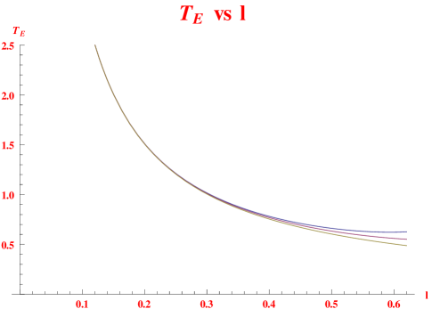
Figure 1: Plots of ‘$T_{E}$ Vs $l$’ for different black hole temperatures (starting from top curve) $T_{Th}=.28,.25,\&.10$ with fixed $\alpha_{0}=.97$ and $(\beta\gamma)^{2}=.5$ for $AdS_{5}$. The graphs split at large $l$ showing the effect of corrections. These demonstrate that $T_{E}$ is higher for higher black hole temperature.

The entanglement energy of subsytem gets corrected as

$$\bigtriangleup{\cal E}^{\ast}=\sqrt{1-{\alpha_{0}}({2\pi\gamma lT_{Th}\over db_{0}})^{d}}\bigtriangleup{\cal E}$$

$$~{}~{}~{}~{}=l\sqrt{1-{\alpha_{0}}({2\pi\gamma lT_{Th}\over db_{0}})^{d}}{L^{d-1}V_{d-3}r_{y}d\over 8G_{d+1}}<t_{00}>$$ (45)

From (39) the chemical potential up to the second order may be written

$$\mu_{\ast}={qa_{2}\over 2r_{y}a_{1}}{\beta\gamma^{2}({2\pi\gamma lT_{Th}\over db_{0}})^{d}}+{\rm~{}higher~{}orders}$$

$$~{}~{}~{}~{}\simeq{qa_{2}\over 2r_{y}\beta a_{1}}(1-{1\over{1+\beta^{2}\gamma^{2}({2\pi\gamma lT_{Th}\over db_{0}})^{d}}})$$ (46)

where the second line merely reflects the fact that any subleading term is a higher order term which can be ignored at the second order. This will lead to following $l$ dependence in the charge

$$\bigtriangleup{\cal N}^{\ast}=l\sqrt{1-{\alpha_{0}}({2\pi\gamma lT_{Th}\over db_{0}})^{d}}~{}{L^{d-1}V_{d-3}r_{y}^{2}d\over 8G_{d+1}}{\beta\gamma^{2}\over z_{0}^{d}}$$ (47)

The large $l$ behaviour may be predicted from here up to some value $l=l_{c}$, such that $l_{c}<{db_{0}\over 2\pi\gamma T_{Th}}$. We cannot stretch these results beyond this bound as this would lead to to the break down of perturbative regime. In large $l$ limit we expect to see the behaviour

$$T_{E}^{\ast}\to T_{Th},~{}~{}~{}~{}\bigtriangleup{\cal E}^{\ast}\to\bigtriangleup{\cal E}_{Th}.$$ (48)

4 Summary

We conclude that the first law of entanglement thermodynamics for ‘boosted’ $AdS_{d+1}$ having black hole in the IR region is given by

$$\bigtriangleup{\cal E}^{\ast}=T_{E}^{\ast}\bigtriangleup S_{E}^{\ast}+\mu_{\ast}\bigtriangleup{\cal N}^{\ast}+{\cal V}_{\ast}\bigtriangleup{\cal P}^{\ast}$$

Our result emphasizes the fact that the form of the first law changes under higher order corrections to the entanglement entropy. It is apparent when the entanglement law (22) at the first order is compared with the second order result in (40). We find that even in the absence of boosts the renormalization of the thermodynamic quantities like entropy, energy, subsystem size (all extensive quantities) and entanglement temperature (intensive quantity) becomes essential at the second order. The chemical potential which is negligible at the first order becomes relevant at next order. We expect no further changes in the form of the first law for the AdS background (1), so the first law form (40) will remain unchanged at higher orders provided we renormalize/redefine the thermodynamic quantities appropriately. Also, we have determined that the entanglement temperature of the subsystem will be higher for a bigger size black hole. Finally, as we have studied (IR) excitations in AdS spacetime, and since AdS background is an universal solution of (gauged) supergravities with negative cosmological constant, we expect these results will be holding true quite generally.

Appendix A Conventions:

The physical observables such as enegry, momentum and pressure can be obtained by expanding the bulk AdS geometry (1) in suitable Feffermann-Graham asymptotic coordinates [8]

$$ds^{2}={L^{2}\over u^{2}}\left({du^{2}}+G^{4\over d}[{-fdt^{2}\over K}+K(dy-\omega)^{2}+dx_{1}^{2}+\cdots+dx_{d-2}^{2}]\right)$$

$$G=1+{u^{d}\over u_{0}^{d}},~{}~{}~{}f\simeq(1-{4u^{d}\over u_{0}^{d}}),~{}~{}~{}K\simeq 1+4\beta^{2}\gamma^{2}{u^{d}\over u_{0}^{d}}$$ (49)

In $u$ coordinate the boundary is at $u=0$, and $u_{0}^{d}=4z_{0}^{d}$. The Kaluza-Klein gauge form is

$$\omega=\beta^{-1}(1-{1\over K})dt.$$ (50)

In these asymptotic coordinates, the coefficients of ${u^{d}}$ terms in the metric expansion give rise to the energy-momentum tensor of the boundary CFT. From (A) these coefficients of the metric are

$$<t_{00}>=({d-1\over d}+\beta^{2}\gamma^{2}){4\over u_{0}^{d}},~{}~{}~{}~{}<t_{0y}>=\beta\gamma^{2}{4\over u_{0}^{d}}$$

$$<t_{11}>={1\over d}{4\over u_{0}^{d}}=<t_{22}>=~{}\cdots$$ (51)

The boundary energy-momentum tensor, $<T_{ab}>={dL^{d-1}\over 16\pi G}<t_{ab}>$, is traceless as we have conformal theory. The energy of excitations and the momentum for the boosted CFT_d will be

$$E={dL^{d-1}v_{d-1}\over 16\pi G_{d+1}}<t_{00}>={dL^{d-1}v_{d-2}r_{y}\over 8G_{d+1}}({d-1\over d}+\beta^{2}\gamma^{2})z_{0}^{-d}$$

$$P_{y}={dL^{d-1}v_{d-2}r_{y}\over 8G_{d+1}}\beta\gamma^{2}z_{0}^{-d}$$ (52)

where volume $v_{d-2}=l_{1}l_{2}\cdots l_{d-2}$, and we have compactified $y$ on a circle of radius $r_{y}$. Note the momentum (charge) $P_{y}={N\over r_{y}}$ is quantized and $N$ would have integral values. In the absence of boost the charge would be vanishing. We note down the nontrivial chemical potential which is defined by the value of gauge potential at the horizon

$$\mu_{Th}={\beta\over r_{y}}$$ (53)

Corresponding thermal entropy and temperature can be obtained from (1). These are given by

$$S_{Th}\equiv{[Area]_{horizon}\over 4G_{d+1}}={\pi L^{d-1}v_{d-2}r_{y}\over 2G_{d+1}}{\gamma\over z_{0}^{d-1}}$$

$$T_{Th}={d\over 4\pi z_{0}\gamma}$$ (54)

These thermal quantities satisfy the following first law of black hole mechanics

$$\delta E_{Th}=T_{Th}\delta S_{Th}+\mu_{{}_{Th}}\delta N\ .$$ (55)

But if we allow small volume changes, say $\delta v=(\delta l_{1})l_{2}l_{3}\cdots l_{d-2}$, the black hole thermodynamic law would be

$$\delta E_{Th}=T_{Th}\delta S_{Th}+\mu_{{}_{Th}}\delta N-{\cal P}_{1}\delta v\ .$$ (56)

where pressure component is ${\cal P}_{1}={L^{d-1}r_{y}\over 8G_{d+1}}z_{0}^{-d}$.

Appendix B Some Beta function Identities

Some useful Beta function integrals we have used are given here

$$b_{0}=\int_{0}^{1}d\xi\xi^{d-1}{1\over\sqrt{R}}={1\over 2(d-1)}B({d\over 2d-2},{1\over 2})$$

$$b_{1}=\int_{0}^{1}d\xi\xi^{2d-1}{1\over\sqrt{R}}={1\over 2(d-1)}B({d\over d-1},{1\over 2})$$

$$b_{2}=\int_{0}^{1}d\xi\xi^{3d-1}{1\over\sqrt{R}}={1\over 2(d-1)}B({3d\over 2d-2},{1\over 2})$$

$$I_{l}=\int_{0}^{1}d\xi\xi^{d-1}(1-\xi^{d}){1\over{R}^{3\over 2}}={d+1\over d-1}b_{1}-{1\over d-1}b_{0}$$

$$J_{l}=\int_{0}^{1}d\xi\xi^{d-1}\left({\beta^{2}\gamma^{2}\over 4}\xi^{d}-{\beta^{4}\gamma^{4}\over 8}(1+3\xi^{d})\right){(1-\xi^{d})\over{R}^{3\over 2}}$$ (57)

where $B(m,n)={\Gamma(m)\Gamma(n)\over\Gamma(m+n)}$ are the Beta-functions. Further integrals are

$$a_{0}=\int_{0}^{1}d\xi\xi^{-d+1}{1\over\sqrt{R}}={1\over 2(d-1)}B({1-d/2\over d-1},{1\over 2})$$

$$a_{1}=\int_{0}^{1}d\xi\xi^{-d+1}{\xi^{d}\over\sqrt{R}}={1\over 2(d-1)}B({1\over d-1},{1\over 2})$$

$$a_{2}=\int_{0}^{1}d\xi\xi^{-d+1}{\xi^{2d}\over\sqrt{R}}={1\over 2(d-1)}B({1+d/2\over d-1},{1\over 2})$$

$$I_{a}=\int_{0}^{1}d\xi\xi^{d-1}(1-\xi^{2d}){1\over{R}^{3/2}}={2d+1\over d-1}b_{2}-{1\over d-1}b_{0}$$ (58)

Some identities we have used are

$$b_{0}=(2-d)a_{0},~{}~{}~{}~{}b_{1}={2\over d+1}a_{1},~{}~{}~{}~{}b_{2}={2+d\over 2d+1}a_{2}\ .$$ (59)

References

- [1] J. Maldacena, Adv. Theor. Math. Phys. 2, 231 (1998) arXiv:9711200[hep-th]; S. Gubser, I Klebanov and A.M. Polyakov, Phys. lett. B 428, 105 (1998) arXiv:9802109[hep-th]; E. Witten, Adv. Theor. Math. Phys. 2, 253 (1998) arXiv:9802150[hep-th].
- [2] S. Ryu and T. Takayanagi, Phys. Rev. Lett. 86 (2006) 181602, arXiv:0603001[hep-th]; S. Ryu and T. Takayanagi, JHEP 0608 (2006) 045, arXiv:0605073[hep-th].
- [3] N. Ogawa, T. Takayanagi, and T. Ugajin, JHEP 1201 (2012) 125, arXiv:1111.1023[hep-th].
- [4] J. Bhattacharya, M. Nozaki, T. Takayanagi and T. Ugajin, Phys. Rev. Lett. 110, no. 9, 091602 (2013) [arXiv:1212.1164].
- [5] D. Allahbakhshi, M. Alishahiha and A. Naseh, JHEP 1308, 102 (2013) [arXiv:1305.2728 [hep-th]].
- [6] D. W. Pang, Phys. Rev. D 88 (2013) 12, 126001 [arXiv:1310.3676 [hep-th]].
- [7] C. Park, Phys. Rev. D 91, no. 12, 126003 (2015) [arXiv:1501.02908 [hep-th]].
- [8] V. Balasubramanian and P. Kraus, Commun. Math. Phys. 208, 413 (1999) [hep-th/9902121]; P. Kraus, F. Larsen and R. Siebelink, Nucl. Phys. B 563, 259 (1999) [hep-th/9906127]; M. Bianchi, D. Z. Freedman and K. Skenderis, Nucl. Phys. B 631, 159 (2002) [hep-th/0112119].
- [9] T. Faulkner, A. Lewkowycz and J. Maldacena, “Quantum corrections to holographic entanglement entropy,” arXiv:1307.2892 [hep-th].
- [10] O. Ben-Ami, D. Carmi and J. Sonnenschein, “Holographic Entanglement Entropy of Multiple Strips,” JHEP 1411, 144 (2014) [arXiv:1409.6305 [hep-th]].