Decay of $B^{\pm}\to\tau^{\pm}+$ “missing momentum” and
direct measurement of the mixing parameter $U_{\tau N}$

Abstract

We derive the decay widths for the leptonic decays of heavy charged pseudoscalars to massive sterile neutrinos, $M^{\pm}\to\ell^{\pm}+N$, within the frameworks involving the Standard Model and two-Higgs doublets (type II). We then apply the result to $B^{\pm}\to\tau^{\pm}+{\rm``missing~{}~{}momentum"}$ of the Belle/BaBar experimental results, in order to measure $directly$ the relevant parameter space, including the mixing parameter $U_{\tau N}$.

I Introduction

The purely leptonic decays $B^{+}\to\ell^{+}\nu$ have been of great interest as a probe for new physics beyond the Standard Model (SM), because in the SM the decay rate can be calculated very precisely and new physics effects, for instance, charged Higgs contributions Hou in the two-Higgs doublet models HHG may appear in the tree-level contribution. In the SM, the decay rates are proportional to $m_{\ell}^{2}$, the square of the corresponding charged lepton mass; therefore the $B^{\pm}$ decays to $e^{\pm}\nu$ and $\mu^{\pm}\nu$ final states are highly suppressed in comparison to $B^{\pm}\to\tau^{\pm}\nu$. Since the first evidence for $B^{\pm}\to\tau^{\pm}\nu$ decays was obtained by the Belle experiment BtotaunuFirst , its branching fraction has been measured by Belle and BaBar BtotaunuBFs , resulting in the world-average value PDG2014

$${\cal B}_{\rm exp}(B^{\pm}\to\tau^{\pm}\nu)=(1.14\pm 0.27)\times 10^{-4}~{}.$$ (1)

This value is consistent with the SM-based prediction,

$${\cal B}_{\rm SM}(B^{\pm}\to\tau^{\pm}\nu)=(0.758_{-0.059}^{+0.080})\times 10^{-4}~{},$$ (2)

which is obtained by fitting the Cabibbo-Kobayashi-Maskawa (CKM) unitarity constraints CKMfitter , at the level of approximately $1.5\sigma$. This implies that if the measurement is improved in future $B$-factory experiments such as Belle II Belle2 , the comparison can clarify whether new physics scenarios are needed.

Heavy sterile neutral particles (also known as “heavy neutrinos”), with suppressed mixing with the sub-eV SM neutrinos, appear in several new physics scenarios, such as the original seesaw seesaw with very heavy neutrinos, seesaw with neutrinos of mass $0.1$-$1$ TeV 1TeVNu , or even scenarios with neutrino mass $\sim 1$ GeV 1GeVNu ; nuMSM ; lowscaleseesaw . We will consider the reaction $B^{\pm}\to\tau^{\pm}N$, where $N$ stands for the heavy neutrino, any heavy sterile neutrino of Dirac type or Majorana type, in interpreting the measured branching fraction in the new physics perspective. Even if $N$ is invisible in the detector, we can still separate $B^{\pm}\to\ell^{\pm}N$ signals from $B^{+}\to\ell^{+}\nu$ for $\ell=e$ or $\mu$, because of the two-body nature of the decay whereby the momentum of the charged lepton in the $B$ meson rest frame is nearly monochromatic and depends on the mass of $N$. The situation is complicated for $B^{\pm}\to\tau^{\pm}N$ because there is more than one neutrino in the final state due to the fast decay of $\tau^{\pm}$, and the decay signature of $B^{\pm}\to\tau^{\pm}N$ becomes almost indistinguishable from the ordinary $B^{\pm}\to\tau^{\pm}\nu$. Therefore, we may not exclude the possibility that the experimentally observed signal of $B^{\pm}\to\tau^{\pm}\nu$ may actually contain contributions from $B^{\pm}\to\tau^{\pm}N$.

Since the measurement of $B^{\pm}\to\tau^{\pm}\nu$ is not only an important CKM unitarity test of the SM, but also a very effective probe into new physics models regarding the charged Higgs, it is important to identify and study any unknown decay modes that can affect the measured branching fraction of $B^{\pm}\to\tau^{\pm}\nu$ as much as we can. In this paper we analyze $B^{\pm}\to\tau^{\pm}N$ both in the SM framework with a minimal extension to include $N$ and in the frameworks involving two-Higgs doublets (type II).

II Decay widths of $B^{\pm}\to\tau^{\pm}+$ “missing momentum” and determination of relevant parameters

Massive neutrinos may be the final state particles of the leptonic decays of the heavy mesons (such as $B^{\pm}$), if such neutrinos mix with the standard flavor neutrinos. If the mixing coefficient for the heavy mass eigenstate $N$ with the standard flavor neutrino $\nu_{\ell}$ ($\ell=e,\mu,\tau$) is denoted as $U_{\ell N}$, then the standard flavor neutrino $\nu_{\ell}$ ($\ell=e,\mu,\tau$) can be represented as

$$\nu_{\ell}=\sum_{k=1}^{3}U_{\ell\nu_{k}}\nu_{k}+U_{\ell N}N\ ,$$ (3)

where $\nu_{k}$ ($k=1,2,3$) denote the light mass eigenstates. In our simplified notation above, we assumed only one additional massive sterile neutrino $N$. The unitary extended Pontekorvo-Maki-Nakagawa-Sakata (PMNS) matrix $U$ Pmns is in this case a $4\times 4$ matrix. However, our formulas, to be derived in this section, will be applicable also to more extended scenarios as well (with more than one additional massive neutrinos $N_{j}$) .

The decay $B^{+}\to\tau^{+}N$ then proceeds via exchange of an (off-shell) $W^{+}$ SM gauge boson. In addition, if the Higgs structure involves two-Higgs doublets, the exchange of the charged Higgs $H^{+}$ also contributes, cf. Figs. 5 (a) and (b), as shown in Appendix A. Straightforward calculation, given in Appendix A, gives us an expression for the decay width $\Gamma(B^{+}\to\tau^{+}N)$; cf. Eq. (23b) in conjunction with Eqs. (20) and (24).

In the decay $B^{+}\to\tau^{+}\nu_{\tau}$, within the SM with $M_{\nu_{\tau}}\approx 0$ and with no charged Higgs, only the decay mode of Fig. 5(a) contributes, and the expression (23b) reduces to

$$\Gamma_{\rm SM}(B^{+}\to\tau^{+}\nu_{\tau})=\frac{1}{8\pi}G_{F}^{2}f_{B}^{2}|V_{ub}|^{2}\left(1-\frac{M_{\tau}^{2}}{M_{B}^{2}}\right)^{2}M_{B}M_{\tau}^{2}\ .$$ (4)

Here, $M_{B}$ and $f_{B}$ are the $B^{+}$ meson mass and the decay constant, respectively, $|V_{ub}|$ is the corresponding CKM matrix element, and $G_{F}$ is the Fermi constant. Using this formula, with the values $f_{B}=0.1906$ GeV (i.e., the central value of $f_{B}=0.1906\pm 0.0047$ GeV Ref. PDG2014 ), $M_{B}=5.279$ GeV and $\tau_{B}=1.638\times 10^{-12}$ s PDG2014 , the SM branching ratio values Eq. (2) from the CKM unitarity constraints CKMfitter would then imply for $|V_{ub}|$ the values $|V_{ub}|=(3.44_{-0.14}^{+0.18})\times 10^{-3}$. It is interesting that these values are very close to the values $|V_{ub}|=(3.23\pm 0.31)\times 10^{-3}$ obtained from exclusive decays $B^{+}\to\pi\ell^{+}\nu$ while the inclusive charmless decays give significantly different values $|V_{ub}|=(4.41\pm 0.22)\times 10^{-3}$ PDG2014 .

If the above decay, with $M_{\nu_{\tau}}\approx 0$, is considered within the two-Higgs doublet model type II [2HDM(II), HHG ], both modes Fig. 5(a) and (b) contribute, and the expression (23b) reduces to

$$\Gamma_{\rm 2HDM(II)}(B^{+}\to\tau^{+}\nu_{\tau})=\frac{1}{8\pi}G_{F}^{2}f_{B}^{2}|V_{ub}|^{2}\left(1-\frac{M_{\tau}^{2}}{M_{B}^{2}}\right)^{2}M_{B}M_{\tau}^{2}r_{H}^{2}=r_{H}^{2}\Gamma_{\rm SM}(B^{+}\to\tau^{+}\nu_{\tau})\ ,$$ (5)

where the factor $r_{H}$ is given in Appendix A in Eq. (20a) which, in the considered case of $B^{+}$ decay, is

$$r_{H}=-1+\frac{M_{B}^{2}}{M_{H}^{2}}\tan^{2}\beta\ ,$$ (6)

where $M_{H}$ is the mass of the charged Higgs $H^{+}$, and $\tan\beta=v_{1}/v_{2}=v_{D}/v_{U}$ is the ratio of the vacuum expectation values of the two Higgs doublets (down type and up type).

Further, if we consider the decay to a massive neutrino $N$, $B^{+}\to\tau^{+}N$, the expressions (4) and (5) get extended due to $M_{N}\not=0$ and due to the mixing factor $U_{\tau N}$ of Eq. (3). However, the expressions (4) and (5) include, in addition to the channels with the first three (almost) massless neutrinos $\nu_{k}$ ($k=1,2,3$), also the spurious channel with a (nonexistent) massless fourth mass eigenstate $N^{\prime}$ whose mixing coefficients are equal to that of the (true) massive $N$, i.e., $U_{\ell N}$. This is due to the unitarity of the $4\times 4$ mixing matrix $U$ appearing in Eq. (3) which implies the relation

$$\sum_{k=1}^{3}|U_{\ell\nu_{k}}|^{2}+|U_{\ell N}|^{2}=1\ .$$ (7)

Therefore, any deviation from the values (4) and (5) due to the existence of a massive neutrino $N$ will be equal to $\Gamma(B^{+}\to\tau^{+}N)-\Gamma(B^{+}\to\tau^{+}N)|_{M_{N}=0}$, where the second term is necessary in order to avoid double counting. We will now simply denote this difference as $\Gamma(B^{+}\to\tau^{+}N)$. According to the general formula (23b), this is then

$$\Gamma_{\rm SM}(B^{+}\to\tau^{+}N)=\frac{1}{8\pi}G_{F}^{2}f_{B}^{2}|V_{ub}|^{2}|U_{\tau N}|^{2}M_{B}M_{\tau}^{2}$$ (8a)

$${\Bigg{\{}}\lambda^{1/2}\left(1,\frac{M_{N}^{2}}{M_{B}^{2}},\frac{M_{\tau}^{2}}{M_{B}^{2}}\right)\frac{1}{M_{B}^{2}M_{\tau}^{2}}\left[(M_{\tau}^{2}+M_{N}^{2})(M_{B}^{2}-M_{N}^{2}-M_{\tau}^{2})+4M_{N}^{2}M_{\tau}^{2}\right]$$

$$-\left(1-\frac{M_{\tau}^{2}}{M_{B}^{2}}\right)^{2}{\Bigg{\}}},$$

$$\Gamma_{\rm 2HDM(II)}(B^{+}\to\tau^{+}N)=\frac{1}{8\pi}G_{F}^{2}f_{B}^{2}|V_{ub}|^{2}|U_{\tau N}|^{2}M_{B}M_{\tau}^{2}$$ (8b)

$${\Bigg{\{}}\lambda^{1/2}\left(1,\frac{M_{N}^{2}}{M_{B}^{2}},\frac{M_{\tau}^{2}}{M_{B}^{2}}\right)\frac{1}{M_{B}^{2}M_{\tau}^{2}}\left[(M_{\tau}^{2}r_{H}^{2}+M_{N}^{2}l_{H}^{2})(M_{B}^{2}-M_{N}^{2}-M_{\tau}^{2})-4r_{H}l_{H}M_{N}^{2}M_{\tau}^{2}\right]$$

$$-\left(1-\frac{M_{\tau}^{2}}{M_{B}^{2}}\right)^{2}r_{H}^{2}{\Bigg{\}}}.$$

The function $\lambda$ appearing here is defined in Appendix A in Eq. (24), and the factor $l_{H}$ in Eq. (20b) which, in the considered case of $B^{+}$ decay, is

$$l_{H}=1+\frac{M_{B}^{2}}{M_{H}^{2}}\ .$$ (9)

The expressions (4) and (8a) should then be added in the SM case, and the expressions (5) and (8b) should be added in the 2HDM(II) case, in order to obtain the full decay widths for $B^{\pm}\to\tau^{\pm}+$ “missing momentum.”

We now summarize three possible cases of numerical interest for the decays $B^{\pm}\to\tau^{\pm}+$ “missing momentum,” all in scenarios beyond the SM:

1. If the missing momenta are only from $\nu_{\tau}$ of the SM, and there is charged Higgs contribution in addition to the SM process, the decay width is determined by Eq. (5). Figure 1 (left panel) shows the allowed regions [shown in dark- and pale-shaded grey (red color online) corresponding to $\pm 1\sigma$ and $\pm 2\sigma$ regions, respectively] in the parameter space of $M_{H}$ and $\tan\beta$ in 2HDM(II). To determine the allowed regions, we compare Eq. (1) for the experimental value with Eq. (2) for the SM contribution in the theory value.

2. If the missing momenta are due to a sterile heavy neutrino as well as the SM tau neutrino, while there being no charged Higgs contribution, the decay width is obtained by adding Eqs. (4) and (8a). Figure 1 (right panel) shows the allowed regions (with the same color assignment as described above) in the parameter space of $M_{N}$ and $|U_{\tau N}|$ assuming no contributions from charged Higgs. Again, to determine these regions we use Eq. (1) for the experimental value and Eq. (2) for the SM contribution in the theory value. We also assume, for this figure, that the sterile heavy particle $N$ is invisible, and hence does not decay inside the detector. Note that the upper bound of the allowed region of $|U_{\tau N}|$ goes beyond 1, which is obviously much larger than the existing upper bound listed in Table 1. This is mainly because the central value of the current world average of ${\cal B}(B^{\pm}\to\tau^{\pm}\nu)$ is significantly larger than the SM-based calculation obtained from the CKM unitarity constraints, Eqs. (1) and (2). The upper bound is less restrictive at low masses $M_{N}$, because the results for the process $B^{\pm}\to\tau^{\pm}+$ “missing momentum” are indistinguishable from those of SM when $M_{N}\to 0$.

   

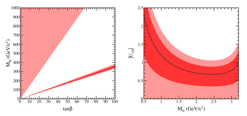
   Figure 1: The allowed regions determined from the measurement of $B^{\pm}\to\tau^{\pm}\nu$ in two cases: (left) the allowed regions in the parameter space of $M_{H^{+}}$ $vs.$ $\tan\beta$ in 2HDM(II) assuming that the missing momenta are only from $\nu_{\tau}$ of the SM; (right) The allowed regions in the parameter space of $M_{N}$ $vs.$ $|U_{\tau N}|$ assuming no contributions from charged Higgs but allowing the possible contributions from heavy neutrino $N$. The dark- and pale-shaded areas (red online) correspond to $\pm 1\sigma$ and $\pm 2\sigma$ allowed regions, respectively.

   Table 1: Presently known upper bound estimates ($cf.$ Ref. Atre ) for $|U_{\ell N}|^{2}$ ($\ell=e,\mu,\tau$) for $M_{N}\approx 1$, $3$ GeV.

   $M_{N}$ [GeV]	$|U_{eN}|^{2}$	$|U_{\mu N}|^{2}$	$|U_{\tau N}|^{2}$
   $\approx 1.0$	$10^{-7}$	$10^{-7}$	$10^{-2}$ (delphi )
   $\approx 3.0$	$10^{-6}$	$10^{-4}$	$10^{-4}$ (delphi )

   One thing we note is that the bound on $|U_{\tau N}|$ in Table 1 has been determined $indirectly$ by DELPHI delphi from the $invisible$ decay width of $Z^{0}$, i.e. $e^{+}e^{-}\to Z^{0}\to N\bar{\nu}$, with $N-\nu_{\tau}$ mixing. Since $\nu_{\tau}$ in this reaction was not explicitly identified, the obtained bound is inclusive of other types of neutrinos. On the other hand, the $B^{\pm}\to\tau^{\pm}\nu$ mode, where $\tau$ is identified, is $directly$ related to $\tau-N$ coupling. Therefore, any information on $|U_{\tau N}|$ obtained from $B^{\pm}\to\tau^{\pm}\nu$ is not influenced by any other types of neutrinos, which makes a clear difference from the DELPHI result. In this regard, even though the current bound on $|U_{\tau N}|$ from ${\cal B}(B^{\pm}\to\tau^{\pm}\nu)$ is much looser than that of DELPHI’s, it will be of great interest if the bound can be improved or evidence for nonzero contribution from $N$ is found in the future measurements of ${\cal B}(B^{\pm}\to\tau^{\pm}\nu)$.

3. If the missing momenta are via a sterile heavy neutrino as well as the SM tau neutrino, and, there is also charged Higgs contribution, the decay width comes from adding Eqs. (5) and (8b). We will discuss this interesting case in details later.

Up until now, a possibly important effect of suppression due to the survival probability was not included. Namely, if the detector has a certain length $L$, the produced massive neutrino $N$ could decay within the detector, producing additional particles. The elimination of such events from the decay width $\Gamma(M^{+}\to\ell^{+}N)$ introduces a suppression factor $S_{N}=\exp[-t/(\tau_{N}\gamma_{N})]$, where $t\approx L/\beta_{N}$ is the time of flight of $N$ through the detector ($\beta_{N}$ being the velocity), and $\gamma_{N}=(1-\beta_{N}^{2})^{-1/2}$ is the time dilation (Lorentz) factor. Therefore, the suppression factor, with which we should multiply the decay width $\Gamma(B^{+}\to\tau^{+}N)$, is thus

$$S_{N}=\exp\left[-\frac{L}{\tau_{N}\gamma_{N}\beta_{N}}\right]\approx\exp\left[-\frac{L\Gamma_{N}}{\gamma_{N}}\right]\ ,$$ (10)

where in the last relation we used $\beta_{N}\approx 1$ and $\tau_{N}=1/\Gamma_{N}$ [$\equiv 1/\Gamma(N\to{\rm all})$], in the units where $c=1=\hbar$.

Following Appendix B, for the decays $B^{\pm}\to\tau^{\pm}N$ and with detectors of length $L\sim 1~{}{\rm m}$, we obtain the following:

• If $M_{N}\approx 1$ GeV: $S_{N}$ is significantly smaller than unity only if the value of $|U_{\tau N}|^{2}$ is close to its present (weakly restricted) upper bound ($|U_{\tau N}|^{2}\sim 10^{-2}$); $S_{N}$ is close to unity otherwise. In our present numerical analysis, we assumed $S_{N}\sim 1$.

• If $M_{N}\approx 3$ GeV: $S_{N}$ is significantly smaller than unity if at least one of the values of the three mixing elements $|U_{\ell^{{}^{\prime}}N}|^{2}$ is close to its present upper bound ($|U_{eN}|^{2}\sim 10^{-6}$, or $|U_{\mu N}|^{2}\sim 10^{-4}$, or $|U_{\tau N}|^{2}\sim 10^{-4}$); $S_{N}$ is close to unity otherwise. In our present numerical analysis, we assumed $S_{N}\sim 1$.

III Numerical Analysis and Discussions

In this Section, we discuss implications from possible future measurements. Although Fig. 1 (right) shows that we can set some constraints on the heavy neutrino mass and its coupling through the measurement of ${\cal B}(B^{\pm}\to\tau^{\pm}\nu)$, the existing uncertainty is too large. Since the Belle II experiment is aiming to increase the data sample by more than a factor of 50, we may expect that the uncertainty of ${\cal B}(B^{\pm}\to\tau^{\pm}\nu)$ can be reduced at least by an order of magnitude. Therefore, in the discussions below, we will assume that the experimental uncertainty is improved by a factor of 10.

First we assume no contribution from charged Higgs such as in 2HDM(II). Consequently, we consider only the diagram shown in Fig. 5(a) in Appendix A where both ordinary $\nu_{\tau}$ and heavy neutral particle $N$ contribute. Depending on the values of $U_{lN}$, $M_{N}$ and the detector size, the produced sterile neutrino $N$ can decay within or beyond the actual detector. When $N$ is produced in the decay $B^{+}\to\tau^{+}N$, and if it decays within the detector, the main signature of $N$ will be $N\to l^{+}\pi^{-}$ (if $N$ is Majorana) or $N\to l^{-}\pi^{+}$ (if $N$ is Dirac or Majorana), which will show experimentally as a resonance in $M(l^{\pm}\pi^{\mp})$. In order to maximize experimental sensitivity, we should analyze both the invisible mode and the visible decay modes for $N$, and combine the corresponding signal yields. Consequently, the value of $U_{lN}$ shall be determined by the combined yields with appropriate corrections for efficiency and subdecay branching fractions. While the invisible mode of $N$ will be analyzed by following the existing $B^{+}\to\tau^{+}\nu_{\tau}$ analyses of Belle and Babar, some of the visible decay modes of $N$ should be explicitly analyzed in the future measurement. Based on our expectation of the branching fractions of the visible modes (see Appendix C) and the survival suppression factor (see Appendix B), the correction factor for the undetected signal events can be obtained for each assumed values of $U_{lN}$ and $m_{N}$.

Figure 2 shows the allowed regions in the parameter space of $M_{N}$ and $|U_{\tau N}|$ in this case. The shaded area (red online) corresponds to $\pm 1\sigma$ (dark) and $\pm 2\sigma$ (pale) allowed regions. For the plot on the left panel, the central value of ${\cal B}(B^{\pm}\to\tau^{\pm}\nu)$ is taken from Ref. PDG2014 , i.e., Eq. (1), but with the uncertainty reduced by a factor of 10. The plot on the right panel assumes that the central value is equal to the value predicted by the CKM unitarity constraint CKMfitter , i.e., Eq. (2), again with tenfold reduction of uncertainty (i.e., $\pm 0.027\times 10^{-4}$). In both cases, the $allowed$ regions are determined by comparing the expected experimental outcome to the theory value, where the SM contribution is taken from Eq. (2).

From Fig. 2 (left), it is evident that we will need an additional contribution from, e.g., $B^{+}\to\tau^{+}N$ if the central value of the current measurement of ${\cal B}(B^{\pm}\to\tau^{\pm}\nu)$ stays the same while a substantial reduction of the measurement uncertainty is achieved. Furthermore, comparison of Fig. 2 (left) with the inclusive upper bound in Table 1 implies that such a scenario would require additional new physics, e.g. 2HDM(II) charged Higgs exchange contributions. Note that, in our numerical analysis that follows, we assume the suppression factor $S_{N}=1$. However, with $|U_{\tau N}|^{2}\sim 10^{-2}$, $\gamma_{N}=2$ and $L=0.1~{}{\rm m}$, we get $S_{N}\sim 1$ (for $M_{N}=1~{}{\rm GeV}$), but $S_{N}\sim 0$ (for $M_{N}=3~{}{\rm GeV}$), which means that the heavy sterile neutrino $N$ is likely to decay within the detector if $M_{N}\gtrsim 3~{}{\rm GeV}$. Therefore, it is important to consider visible decay modes of $N$ as well as the invisible mode.

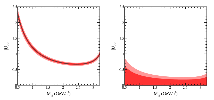
Figure 2: The allowed regions in the parameter space of $M_{N}$ and $|U_{\tau N}|$ assuming no contributions from charged Higgs, where the $\pm 1\sigma$ and $\pm 2\sigma$ allowed regions are displayed by dark and pale shades (red online), respectively: (left) the central value of ${\cal B}(B^{\pm}\to\tau^{\pm}\nu)$ is taken as the current world average Eq. (1), while tenfold reduction of uncertainty is assumed; (right) the central value is taken to be the value predicted by the CKM unitarity constraint, also assuming tenfold reduction of experimental uncertainty. In all cases, the comparison is made to the value determined from the CKM unitarity fitting Eq. (2).

On the other hand, if we consider the case where there is no contribution from unknown heavy neutrino $N$, we note that the parameters $M_{H^{+}}$ and $\tan\beta$ can be much further constrained if the ${\cal B}(B^{\pm}\to\tau^{\pm}\nu)$ uncertainty is improved, e.g. by a factor of 10. Figure 3 shows the allowed regions in the parameter space of $M_{H^{+}}$ vs $\tan\beta$ of 2HDM (type II) while assuming no contributions from heavy neutral particle $N$. The $\pm 1\sigma$ and $\pm 2\sigma$ allowed regions are displayed by dark and pale shades (red online), respectively. The left panel plot uses, for the central value of ${\cal B}(B^{\pm}\to\tau^{\pm}\nu)$, the current world average and assumes tenfold reduction of uncertainty. For the right panel plot, we consider the case of the central value being identical with the present value predicted by the CKM unitarity constraint and the experimental uncertainty is reduced by a factor of 10 compared to the current value $\pm 0.27\times 10^{-4}$. In both cases, the comparison is made to the value determined from the CKM unitarity constraints Eq. (2). Figure 3 (left) shows that 2HDM(II), for each $\tan\beta$, has a very narrow interval of the corresponding allowed values of $M_{H}=M_{H}(\beta)$ if the central experimental value of ${\cal B}(B^{\pm}\to\tau^{\pm}\nu)$ remains approximately unchanged and the experimental uncertainty is reduced tenfold.

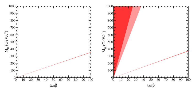
Figure 3: The allowed regions in the parameter space of $M_{H^{+}}$ $vs.$ $\tan\beta$ in 2HDM (type II), assuming no contributions from heavy neutral particle $N$, where the $\pm 1\sigma$ and $\pm 2\sigma$ allowed regions are displayed by dark and pale shades (red online), respectively: (left) the central value of ${\cal B}(B^{\pm}\to\tau^{\pm}\nu)$ is taken from the current world average, while tenfold reduction of uncertainty is assumed; (right) the central value is taken to be the value predicted by the CKM unitarity constraint, also assuming tenfold reduction of experimental uncertainty. In both cases, the comparison is made to the value determined from the CKM unitarity constraints Eq. (2).

Now, let’s consider the case where both charged Higgs $H^{\pm}$ and heavy neutrino $N$ contribute to the measurement of $B^{\pm}\to\tau^{\pm}\nu$, based on the decay rates of Eqs. (5) and (8b). Figure 4 shows a few exemplary cases. As in the cases of Fig. 2, we assume, in Fig. 4, that both invisible and visible decays of $N$ are analyzed with appropriate corrections being applied to the signal yields to obtain the necessary branching fraction. For each of the two plots in the top panel, we choose a point in the parameter space of $M_{N}$ ${\rm vs}$ $|U_{\tau N}|$ and show the allowed region in the parameter space of $M_{H^{+}}$ and $\tan\beta$. For the bottom panel, we choose points in the space of $M_{H^{+}}$ ${\rm vs}$ $\tan\beta$ and show the allowed region in $|U_{\tau N}|$ ${\rm vs}$ $M_{N}$. The two plots in the left panel correspond to the case where we choose points within the allowed region, while we choose points outside the allowed region for the two plots in the right panel. For Fig. 4(a), we choose $M_{N}=1.0~{}{\rm GeV}/c^{2}$ and $|U_{\tau N}|=0.6$. On the other hand, for Fig. 4(b) we choose $M_{N}=1.0~{}{\rm GeV}/c^{2}$ and $|U_{\tau N}|=0.5$. Although it may seem a small difference between the two cases, the resulting allowed regions shown in the $M_{H^{+}}$-vs-$\tan\beta$ space is clearly different. Similarly, we choose $M_{H^{+}}=200~{}{\rm GeV}/c^{2}$ for both plots in the bottom panel of Fig. 4, but $\tan\beta=56.5$ (allowed) for the left and $\tan\beta=55$ (excluded) for the right. Again, we see clear difference between the two cases.

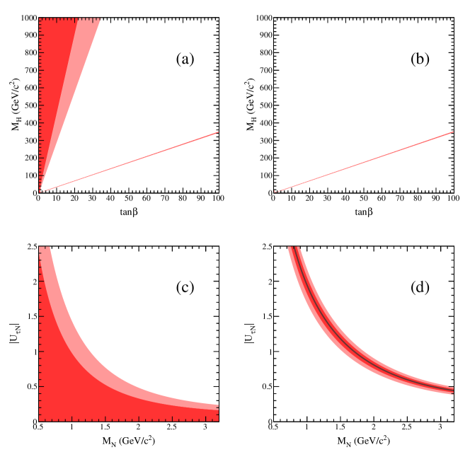
Figure 4: The allowed regions under the assumption that both $H^{+}$ and $N$ contribute to the measured value of $B^{\pm}\to\tau^{\pm}\nu$, based on the decay rates of Eqs. (5) and (8b). Top left: the allowed region in the parameter space of $M_{H^{+}}$ and $\tan\beta$ when $M_{N}=1.0~{}{\rm GeV}/c^{2}$ and $|U_{\tau N}|=0.6$. Top right: the allowed region when $M_{N}=1.0~{}{\rm GeV}/c^{2}$ and $|U_{\tau N}|=0.5$. Bottom left: the allowed region in the parameter space of $|U_{\tau N}|$ and $M_{N}$ when $M_{H^{+}}=200~{}{\rm GeV}/c^{2}$ and $\tan\beta=56.5$. Bottom right: the allowed region when $M_{H^{+}}=200~{}{\rm GeV}/c^{2}$ and $\tan\beta=55$.

IV Summary and Prospects

We have seen, in Figs. 1-4, that the existing measurements of $B^{\pm}\to\tau^{\pm}\nu$ can be reinterpreted by including the possible contributions from a heavy neutral sterile particle $N$. However, with the current experimental uncertainty, the case is not clear yet. On the other hand, with the upcoming next-generation measurements from flavor physics facilities such as Belle II, the experimental uncertainty can be greatly reduced, as was indicated in Figs. 2-4. In that case we can set interesting constraints on parameters of 2HDM(II) and on heavy neutrino $N$ in the range $M_{N}\lesssim 3~{}{\rm GeV}/c^{2}$. For instance, if the current experimental average value of ${\cal B}(B^{\pm}\to\tau^{\pm}\nu)$ stays approximately the same but the experimental uncertainties are greatly reduced, it can be a strong indication that we may need a charged Higgs such as in 2HDM(II), and/or possibly a heavy neutrino $N$.

In the decays $B^{\pm}\to\ell^{\pm}+N$ when $\ell=e$ or $\mu$, the problems of double counting encountered in Sec. II do not appear, because the kinematics allows to distinguish such decays from those of $B^{\pm}\to\ell^{\pm}+\nu_{k}$ ($k=1,2,3$) as mentioned in the Introduction. The relevant formulas for such cases are thus

$$\Gamma_{\rm SM}(B^{+}\to\ell^{+}N) = \frac{1}{8\pi}G_{F}^{2}f_{B}^{2}|V_{ub}|^{2}|U_{\ell N}|^{2}\lambda^{1/2}\left(1,\frac{M_{N}^{2}}{M_{B}^{2}},\frac{M_{\ell}^{2}}{M_{B}^{2}}\right)$$

$$\times\frac{1}{M_{B}}\left[(M_{\ell}^{2}+M_{N}^{2})(M_{B}^{2}-M_{N}^{2}-M_{\ell}^{2})+4M_{N}^{2}M_{\ell}^{2}\right],\,$$

$$\Gamma_{\rm 2HDM(II)}(B^{+}\to\ell^{+}N) = \frac{1}{8\pi}G_{F}^{2}f_{B}^{2}|V_{ub}|^{2}|U_{\ell N}|^{2}\lambda^{1/2}\left(1,\frac{M_{N}^{2}}{M_{B}^{2}},\frac{M_{\ell}^{2}}{M_{B}^{2}}\right)\frac{1}{M_{B}}$$

$$\times\left[(M_{\ell}^{2}r_{H}^{2}+M_{N}^{2}l_{H}^{2})(M_{B}^{2}-M_{N}^{2}-M_{\ell}^{2})-4r_{H}l_{H}M_{N}^{2}M_{\ell}^{2}\right]\ ,$$

where $\ell=e$ or $\mu$. Although the mass of $\ell$ is in this case small or almost zero implying the helicity suppression in the three-generation case, the presence of a massive neutrino $M_{N}\sim 1$ GeV may make the decays (11) appreciable, depending certainly on the mixing strength $|U_{\ell N}|^{2}$. In the $e^{+}e^{-}$ $B$-factory experiments where $B$ mesons are produced via $e^{+}e^{-}\to\Upsilon(4S)\to B\overline{B}$ process, the presence of heavy neutrino $N$ in the decays $B^{+}\to\ell^{+}N~{}(\ell=e,\mu)$ will be distinguishable from $B^{+}\to\ell^{+}\nu_{\ell}$ by the momentum of $\ell^{+}$ in the rest frame of $B^{+}$.

This study can be also extended to other decay modes such as $B\to D^{(*)}\tau^{+}\nu$ and $B^{+}\to\ell^{+}\nu$ ($\ell=e$ or $\mu$). By combining $B^{\pm}\to\tau^{\pm}\nu$ and $B\to D^{(*)}\tau^{+}\nu$ together, the sensitivity of searching for $N$ can be even more enhanced. Moreover, it is expected that $B^{\pm}\to\mu^{\pm}\nu$ decays can be observed in the Belle II experiment. This decay, unlike $B^{\pm}\to\tau^{\pm}\nu$, is a two-body decay mode of $B^{\pm}$; hence the final-state charged lepton ($\mu^{\pm}$) has a nearly monoenergetic distribution in the rest frame of the $B$ meson. If a heavy neutrino $N$, in addition to $\nu_{\mu}$ of SM, also contributes to this decay, it will change the energy distribution of $\mu^{\pm}$ and its effect can be measured experimentally. In the case of $B^{\pm}\to e^{\pm}\nu$, the SM expectation is very low, well beyond the sensitivity of Belle II. Nevertheless, if a heavy neutrino exists and contributes to $B^{\pm}\to e^{\pm}\nu$, it can enhance the branching fraction to be within the experimental sensitivity of Belle II.

Appendix A Derivation of the Decay Widths $\Gamma(M^{\pm}\to\ell^{\pm}N)$

Figure 5: The decay $M^{+}\to N\ell^{+}$ via the exchange of (a) $W^{+}$ and (b) $H^{+}$.

In this Appendix, we derive the decay width of the process $M^{+}\to\ell^{+}N$ of Figs. 5(a) and 5 (b). The first decay mode Fig. 5(a), involves an exchange of (off-shell) $W^{+}$. Direct calculation gives for the contribution ${\cal T}^{(W)}$ of the $W^{+}$ exchange to the reduced scattering (decay) matrix (assuming $M_{W}\gg M_{M}$)

$${\cal T}^{(W)}=U^{*}_{\ell N}V^{*}_{UD}\frac{G_{F}}{\sqrt{2}}\langle 0|{\overline{D}}\gamma^{\eta}(1-\gamma_{5})U|M^{+}\rangle\left[{\overline{u}}_{N}\gamma_{\eta}(1-\gamma_{5})v_{\ell}\right]\ ,$$ (12)

where ${\overline{D}}$ and $U$ denote the two valence quarks of the pseudoscalar meson $M^{+}$, $V_{UD}$ is the corresponding CKM mixing matrix element, and $G_{F}=(1/(4\sqrt{2}))(g/M_{W})^{2}=1.166\times 10^{-5}\ {\rm GeV}^{-2}$ .

In the model with 2HDM(II), the couplings of the charged Higgses $H^{\pm}$ with fermions are similar to those of $W^{\pm}$ HHG . The relevant parts of the Lagrange density are

$${\cal L}_{H^{\pm}qq} = \frac{g}{2\sqrt{2}M_{W}}\sum_{j,k}H^{+}V_{U_{j}D_{k}}\left[\cot\beta{\overline{U}}_{j}M_{U_{j}}(1-\gamma_{5})D_{k}+\tan\beta{\overline{U}}_{j}M_{D_{k}}(1+\gamma_{5})D_{k}\right]$$ (13a)

$$+{\rm H.c.}\ ,$$

$${\cal L}_{H^{\pm}N\ell} = \frac{g}{2\sqrt{2}M_{W}}\sum_{\ell}H^{+}U^{*}_{\ell N}\left[\cot\beta{\overline{N}}M_{N}(1-\gamma_{5})\ell+\tan\beta{\overline{N}}M_{\ell}(1+\gamma_{5})\ell\right]$$ (13b)

$$+{\rm H.c.}\ .$$

The first density is for the coupling with quarks, and the second for the the coupling with the sterile massive neutrino $N$ and the three charged leptons $(\ell=e,\mu,\tau$). Here, $\tan\beta=v_{1}/v_{2}=v_{D}/v_{U}$ is the ratio of the vacuum expectation values of the two-Higgs doublets (down type and up type).

In analogy with the case of $W^{+}$ exchange, we obtain the contribution ${\cal T}^{(H)}$ of the $H^{+}$ exchange to the reduced scattering (decay) matrix ${\cal T}$ (assuming $M_{H}\gg M_{M}$)

$${\cal T}^{(H)} = U^{*}_{\ell N}V^{*}_{UD}\frac{G_{F}}{\sqrt{2}}(-1)\frac{1}{M_{H}^{2}}\left[\langle 0|{\overline{D}}(1-\gamma_{5})U|M^{+}\rangle m_{D}\tan\beta+\langle 0|{\overline{D}}(1+\gamma_{5})U|M^{+}\rangle m_{U}\cot\beta\right]$$ (14)

$$\times\left\{\left[{\overline{u}}_{N}(1-\gamma_{5})v_{\ell}\right]M_{N}\cot\beta+\left[{\overline{u}}_{N}(1+\gamma_{5})v_{\ell}\right]M_{\ell}\tan\beta\right\}\ ,$$

where $M_{H}$ is the mass of $H^{+}$.

The expressions (12) and (14) can be further simplified by the axial-vector current and pseudoscalar relations

$$\langle 0|{\overline{D}}\gamma^{\eta}(1-\gamma_{5})U|M^{+}\rangle = if_{M}p_{M}^{\eta}\ ,$$ (15a)

$$\langle 0|{\overline{D}}(1\mp\gamma_{5})U|M^{+}\rangle = \mp if_{M}\frac{M_{M}^{2}}{m_{D}}\ ,$$ (15b)

where $f_{M}$, $M_{M}$ and $p_{M}$ are the decay constant, mass and 4-momentum of $M^{+}$, respectively. In Eq. (15b), the mass of $m_{U}$ was neglected in comparison with $m_{D}$. For example, for $B^{+}$ we have $D=b$ and $U=u$.

Using the relation (15a) in the expression (12), and using the relations

$${\displaystyle{\not}p_{M}} = {\displaystyle{\not}p_{N}}+{\displaystyle{\not}p_{\ell}}\ ,$$ (16a)

$${\overline{u}}_{N}\displaystyle{\not}p_{N} = M_{N}{\overline{u}}_{N}\ ,\quad\displaystyle{\not}p_{\ell}v_{\ell}=-M_{\ell}v_{\ell}\ ,$$ (16b)

we obtain the following form for the reduced scattering (decay) matrix element for the $W^{+}$-mediated decay:

$${\cal T}^{(W)}=if_{M}U^{*}_{\ell N}V^{*}_{UD}\frac{G_{F}}{\sqrt{2}}\left\{+M_{N}\left[{\overline{u}}_{N}(1-\gamma_{5})v_{\ell}\right]-M_{\ell}\left[{\overline{u}}_{N}(1+\gamma_{5})v_{\ell}\right]\right\}\ .$$ (17)

Using the relation (15b) in the expression (14), and neglecting there the term proportional to $m_{U}\cot\beta$ ($\ll m_{D}\tan\beta$), the reduced scattering (decay) matrix element for the $H^{+}$-mediated decay becomes

$${\cal T}^{(H)} = if_{M}U^{*}_{\ell N}V^{*}_{UD}\frac{G_{F}}{\sqrt{2}}\frac{M_{M}^{2}}{M_{H}^{2}}\tan\beta$$ (18)

$$\times\left\{\left[{\overline{u}}_{N}(1-\gamma_{5})v_{\ell}\right]M_{N}\cot\beta+\left[{\overline{u}}_{N}(1+\gamma_{5})v_{\ell}\right]M_{\ell}\tan\beta\right\}\ .$$

Combining Eqs. (17) and (18), we obtain finally the reduced scattering (decay) matrix element ${\cal T}$ for the decay $M^{+}\to N\ell^{+}$

$${\cal T} = {\cal T}^{(W)}+{\cal T}^{(H)}$$ (19a)

$$= if_{M}U^{*}_{\ell N}V^{*}_{UD}\frac{G_{F}}{\sqrt{2}}\left\{\left[{\overline{u}}_{N}(1+\gamma_{5})\right]M_{\ell}r_{H}+\left[{\overline{u}}_{N}(1-\gamma_{5})\right]M_{N}l_{H}\right\}\ ,$$

where the coefficients are

$$r_{H} = -1+\frac{M_{M}^{2}}{M_{H}^{2}}\tan^{2}\beta\ ,$$ (20a)

$$l_{H} = +1+\frac{M_{M}^{2}}{M_{H}^{2}}\ .$$ (20b)

The square of this matrix element (summed over the helicities of the two final particles) then gives

$$\langle|{\cal T}|^{2}\rangle=4G_{F}^{2}f_{M}^{2}|U_{\ell N}|^{2}|V_{UD}|^{2}\left[(M_{\ell}^{2}r_{H}^{2}+M_{N}^{2}l_{H}^{2})(p_{N}\cdot p_{\ell})-2r_{H}l_{H}M_{\ell}^{2}M_{N}^{2}\right]\ ,$$ (21)

where we have

$$(p_{N}\cdot p_{\ell})=\frac{1}{2}(M_{M}^{2}-M_{N}^{2}-M_{\ell}^{2})\ .$$ (22)

In the rest frame of $M^{+}$ we then have for the decay width

$$\Gamma(M^{+}\to\ell^{+}N)=\frac{1}{16\pi M_{M}}\lambda^{1/2}\left(1,\frac{M_{N}^{2}}{M_{M}^{2}},\frac{M_{\ell}^{2}}{M_{M}^{2}}\right)\langle|{\cal T}|^{2}\rangle$$ (23b)

$$= \frac{1}{8\pi}G_{F}^{2}f_{M}^{2}|U_{\ell N}|^{2}|V_{UD}|^{2}\lambda^{1/2}\left(1,\frac{M_{N}^{2}}{M_{M}^{2}},\frac{M_{\ell}^{2}}{M_{M}^{2}}\right)$$

$$\times\frac{1}{M_{M}}\left[(M_{\ell}^{2}r_{H}^{2}+M_{N}^{2}l_{H}^{2})(M_{M}^{2}-M_{N}^{2}-M_{\ell}^{2})-4r_{H}l_{H}M_{N}^{2}M_{\ell}^{2}\right]\ ,$$

where we used the notation

$$\lambda(y_{1},y_{2},y_{3})=y_{1}^{2}+y_{2}^{2}+y_{3}^{2}-2y_{1}y_{2}-2y_{2}y_{3}-2y_{3}y_{1}\ .$$ (24)

The expression (23b), in conjunction with the expressions (20) and (24), is the explicit expression for the decay width $\Gamma(M^{+}\to N\ell^{+})$ in the rest frame of $M^{+}$, in terms of the masses $M_{M}$, $M_{N}$, $M_{\ell}$, $M_{H}$ and $\tan\beta\equiv v_{U}/v_{D}$.

It is straightforward to check that in the case of $M_{N}=0$ and $|U_{\ell N}|=1$, the obtained formula (23b) reduces to the formula obtained in Ref. Hou . Further, if $M_{H}\to\infty$ (i.e., no charge Higgs interchange), the formula (23b) reduces to Eq. (2.5) of Ref. CDK .

Appendix B Survival Suppression Factor

We first mention that the factor of “nonsurvival” probability $P_{N}=1-S_{N}$ has been discussed and investigated in the literature for the processes where the intermediate on-shell particle (such as $N$) is assumed to decay within the detector, cf. Refs. Gronau ; CDK ; scatt3 ; CKZ1 ; Kimcomm ; CKZ2 ; CDKZ ; CERN-SPS . Here in this Section we follow the notations and results of Ref. CKZ2 . The total decay width $\Gamma_{N}$ of sterile massive neutrino $N$ appearing in Eq. (10) can be expressed as

$$\Gamma_{N}={\overline{\Gamma}}(M_{N}){\widetilde{\cal K}}\ ,$$ (25)

where

$${\overline{\Gamma}}(M_{N})\equiv\frac{G_{F}^{2}M_{N}^{5}}{96\pi^{3}}\ ,$$ (26)

and the factor ${\widetilde{\cal K}}$ is proportional to the heavy-light mixing factors $|U_{\ell^{{}^{\prime}}N}|^{2}$ [where $U_{\ell^{{}^{\prime}}N}$ appear in the relation (3)]

$${\widetilde{\cal K}}(M_{N})\equiv{\widetilde{\cal K}}={\cal N}_{eN}\;|U_{eN}|^{2}+{\cal N}_{\mu N}\;|U_{\mu N}|^{2}+{\cal N}_{\tau N}\;|U_{\tau N}|^{2}\ .$$ (27)

Here, the coefficients ${\cal N}_{\ell^{{}^{\prime}}N}(M_{N})\equiv{\cal N}_{\ell^{{}^{\prime}}N}$ ($\ell^{{}^{\prime}}=e,\mu,\tau$) are the effective mixing coefficients. We have ${\cal N}_{\ell^{{}^{\prime}}N}\sim 10^{0}$-$10^{1}$. They are functions of the mass $M_{N}$ and were numerically evaluated in Ref. CKZ2 for the Majorana neutrino $N$, on the basis of formulas of Ref. HKS . The numerical results for the Dirac $N$ were included in Ref. CDKZ .

In the ranges of $M_{N}$ typical for the $B^{\pm}\to N\ell^{\pm}$ decays, i.e., for $M_{N}\approx 1$-$4$ GeV, we have ${\cal N}_{eN}\approx{\cal N}_{\mu N}\approx 8$ and ${\cal N}_{\tau N}\approx 3$, and therefore

$${\widetilde{\cal K}}\approx 8(|U_{eN}|^{2}+|U_{\mu N}|^{2})+3|U_{\tau N}|^{2}\quad(B,B_{c}\;{\rm decays})\ .$$ (28)

The estimate (28) is valid for Majorana $N$. For Dirac $N$ it is somewhat lower, but the difference can be ignored at the level of precision of the estimate, for $1\ {\rm GeV}\leq M_{N}\leq 3\ {\rm GeV}$.

We refer to Ref. CKZ2 (and references therein) for more details on these results. Furthermore, approximate values of the presently known upper bounds for the squares of the mixing elements, in this range of masses $M_{N}$, are given in Table 1 (cf. Ref. Atre ).

The survival factor (10) can be rewritten as

$$S_{N}=\exp\left(-\frac{L}{L_{N}}\right)=\exp\left(-\frac{L}{{{\overline{L}}}_{N}}{\widetilde{\cal K}}\right)\ ,$$ (29)

where $L_{N}$ is the decay length, and ${{\overline{L}}}_{N}$ is the canonical decay length (canonical in the sense that it is independent of the mixing parameters $U_{\ell^{{}^{\prime}}N}$)

$$L_{N}^{-1} = {{\overline{L}}}_{N}^{-1}{\widetilde{\cal K}}\ ,$$ (30a)

$${{\overline{L}}}_{N}^{-1} = \frac{{\overline{\Gamma}}(M_{N})}{\gamma_{N}}\ ,$$ (30b)

where ${\overline{\Gamma}}(M_{N})$ is given in Eq. (26). The inverse canonical decay length ${\overline{L}}_{N}^{-1}$, for $\gamma_{N}=2$, is given in Fig. 6 as a function of $M_{N}$. Specifically, we obtain ${\overline{L}}_{N}^{-1}\approx 10^{2}\ {\rm m}^{-1}$, $3\times 10^{4}\ {\rm m}^{-1}$, for $M_{N}=1$ GeV, $3$ GeV, respectively. Combining this result with the results (28) and Table 1, we obtain for the effective inverse decay length $L_{N}^{-1}$ [appearing in the survival factor $S_{N}$ of Eq. (29)] the following estimates, in units of $m^{-1}$:

$$L_{N}^{-1}(M_{N}\approx 1{\rm GeV}) \approx 0.8\times 10^{3}|U_{eN_{j}}|^{2}+0.8\times 10^{3}|U_{\mu N_{j}}|^{2}\quad(+2\times 10^{2}|U_{\tau N_{j}}|^{2})$$ (31a)

$$\lesssim 10^{-4}+10^{-4}\quad(+10^{0})\ ,$$

$$L_{N}^{-1}(M_{N}\approx 3{\rm GeV}) \approx 3\times 10^{5}|U_{eN_{j}}|^{2}+3\times 10^{5}|U_{\mu N_{j}}|^{2}\quad(+1\times 10^{5}|U_{\tau N_{j}}|^{2})$$ (31b)

$$\lesssim 10^{0}+10^{0}\quad(+10^{0})\ .$$

Figure 6: The inverse canonical decay length ${\overline{L}}_{N}^{-1}\equiv{\overline{\Gamma}}(M_{N})/\gamma_{N}$, in units of $m^{-1}$, as a function of the neutrino mass $M_{N}$, for the choice $\gamma_{N}$ [$\equiv(1-\beta_{N}^{2})^{-1/2}$] $=2$.

Appendix C Branching ratios for semihadronic decays of neutrino

Here we summarize some of the formulas for the decay widths and branching ratios for the decays of a heavy neutrino $N$ into hadrons Atre ; HKS . Comparatively appreciable channels are decays into light mesons (with mass $M_{H}<1$ GeV), which can be presudoscalar (P) or vector (V) mesons:

$$2\Gamma(N\to\ell^{-}P^{+}) = |B_{\ell N}|^{2}\frac{G_{F}^{2}}{8\pi}M_{N}^{3}f_{P}^{2}|V_{P}|^{2}F_{P}(x_{\ell},x_{P})\$$ (32a)

$$\Gamma(N\to\nu_{\ell}P^{0}) = |B_{\ell N}|^{2}\frac{G_{F}^{2}}{64\pi}M_{N}^{3}f_{P}^{2}(1-x_{P}^{2})^{2}\$$ (32b)

$$2\Gamma(N\to\ell^{-}V^{+}) = |B_{\ell N}|^{2}\frac{G_{F}^{2}}{8\pi}M_{N}^{3}f_{V}^{2}|V_{V}|^{2}F_{V}(x_{\ell},x_{V})\$$ (32c)

$$\Gamma(N\to\nu_{\ell}V^{0}) = |B_{\ell N}|^{2}\frac{G_{F}^{2}}{2\pi}M_{N}^{3}f_{V}^{2}\kappa_{V}^{2}(1-x_{V}^{2})^{2}(1+2x_{V}^{2}).$$ (32d)

Here, $\ell=e,\mu,\tau$ stands generically for a charged lepton. The charged meson channels above were multiplied by a factor $2$, because if $N$ is Majorana neutrino both decays $N\to\ell^{-}M^{+}$ and $N\to\ell^{+}M^{-}$ contribute ($M=P,V$) equally. The factors $f_{P}$ and $f_{V}$ are the decay constants, and $V_{P}$ and $V_{V}$ are the CKM matrix elements involving the valence quarks of the corresponding mesons.

In Eqs. (32), the following notation is used: $x_{Y}\equiv M_{Y}/M_{N}$ ($Y=\ell,P,V$), and the expressions $F_{P}$ and $F_{V}$ are

$$F_{P}(x,y) = \lambda^{1/2}(1,x^{2},y^{2})\left[(1+x^{2})(1+x^{2}-y^{2})-4x^{2}\right]\$$ (33a)

$$F_{V}(x,y) = \lambda^{1/2}(1,x^{2},y^{2})\left[(1-x^{2})^{2}+(1+x^{2})y^{2}-2y^{4}\right]\ ,$$ (33b)

where

$$\lambda(y_{1},y_{2},y_{3})=y_{1}^{2}+y_{2}^{2}+y_{3}^{2}-2y_{1}y_{2}-2y_{2}y_{3}-2y_{3}y_{1}\ .$$ (34)

The (light) mesons for which formulas (32) can be applied are: $P^{\pm}=\pi^{\pm},K^{\pm}$; $P^{0}=\pi^{0},K^{0},{\bar{K}}^{0},\eta$; $V^{\pm}=\rho^{\pm},K^{*\pm}$; $V^{0}=\rho^{0},\omega,K^{*0},{\bar{K}}^{*0}$. If $M_{N}>1$ GeV, the neutrino $N$ can decay into heavier mesons, and the decay widths for such decays can be calculated by using duality, as decay widths into quark pairs; nonetheless, such decay modes are in general suppressed by kinematics and are not given here. The corresponding branching ratios are obtained by dividing the above decay widths by the total decay width $\Gamma_{N}$ of $N$.

References

(1)
W. S. Hou,
Phys. Rev. D 48, 2342 (1993).
(2)
J. F. Gunion, H. E. Haber, G. Kane and S. Dawson, The Higgs Hunter’s Guide , Perseus Publishing, Cambridge, Massachusetts, 1990.
(3) K. Ikado et al. (Belle Collab.) Phys. Rev. Lett. 97, 251802 (2006).
(4)
K. Hara et al. (Belle Collab.), Phys. Rev. Lett. 110,
131801 (2013);
J.P. Lees et al. (BaBar Collab.), Phys. Rev. D 88,
031102(R) (2013);
B. Aubert et al. (BaBar Collab.), Phys. Rev. D 81,
051101(R) (2010);
K. Hara et al. (Belle Collab.), Phys. Rev. D 82,
071101(R) (2010).
(5) K.A. Olive et al. (Particle Data Group),
Chin. Phys. C, 38, 090001 (2014).
(6) J. Charles, A. Höcker, H. Lacker, S. Laplace, F. R. Diberder, J. Malclés, J. Ocariz, M. Pivk, and L. Rook (CKMfitter Group), Eur. Phys. J. C 41, 1-131 (2005) , updated results and
plots available at: http://ckmfitter.in2p3.fr
(7)
T. Abe et al., arXiv:1011.0352v1.
(8)
P. Minkowski,
Phys. Lett. B 67, 421 (1977);
M. Gell-Mann, P. Ramond and R. Slansky, Caltech preprint CALT-68-700, Febr. 1979, arXiv:hep-ph/9809459;
in , editied by D. Reedman et al. (North-Holland, Amsterdam, 1979);
T. Yanagida,
Conf. Proc. C 7902131, 95 (1979);
S. L. Glashow, in : edited by M. Lévy et al. (Plenum, New York, 1980), p. 707;
R. N. Mohapatra and G. Senjanović,
Phys. Rev. Lett. 44, 912 (1980).
(9)
D. Wyler and L. Wolfenstein,
Nucl. Phys. B 218, 205 (1983);
E. Witten,
Nucl. Phys. B 258, 75 (1985);
R. N. Mohapatra and J. W. F. Valle,
Phys. Rev. D 34, 1642 (1986);
A. Pilaftsis and T. E. J. Underwood,
Phys. Rev. D 72, 113001 (2005)
[hep-ph/0506107];
M. Malinsky, J. C. Romao and J. W. F. Valle,
Phys. Rev. Lett. 95, 161801 (2005)
[hep-ph/0506296];
P. S. Bhupal Dev and R. N. Mohapatra,
Phys. Rev. D 81, 013001 (2010)
[arXiv:0910.3924 [hep-ph]];
P. S. B. Dev and A. Pilaftsis,
Phys. Rev. D 86, 113001 (2012)
[arXiv:1209.4051 [hep-ph]];
C. H. Lee, P. S. Bhupal Dev and R. N. Mohapatra,
Phys. Rev. D 88, 093010 (2013)
[arXiv:1309.0774 [hep-ph]];
A. Das and N. Okada,
Phys. Rev. D 88, 113001 (2013)
[arXiv:1207.3734 [hep-ph]];
A. Das, P. S. Bhupal Dev and N. Okada,
Phys. Lett. B 735, 364 (2014)
[arXiv:1405.0177 [hep-ph]].
(10)
W. Buchmüller and C. Greub,
Nucl. Phys. B 363, 345 (1991);
J. Kersten and A. Y. Smirnov,
Phys. Rev. D 76, 073005 (2007)
[arXiv:0705.3221 [hep-ph]];
F. del Aguila, J. A. Aguilar-Saavedra, J. de Blas and M. Zralek,
Acta Phys. Polon. B 38, 3339 (2007)
[arXiv:0710.2923 [hep-ph]];
X. G. He, S. Oh, J. Tandean and C. C. Wen,
Phys. Rev. D 80, 073012 (2009)
[arXiv:0907.1607 [hep-ph]];
A. Ibarra, E. Molinaro and S. T. Petcov,
J. High Energy Phys. 1009 (2010) 108
[arXiv:1007.2378 [hep-ph]].
(11)
T. Asaka, S. Blanchet and M. Shaposhnikov,
Phys. Lett. B 631, 151 (2005)
[hep-ph/0503065];
T. Asaka and M. Shaposhnikov,
Phys. Lett. B 620, 17 (2005)
[hep-ph/0505013];
D. Gorbunov and M. Shaposhnikov,
J. High Energy Phys. 0710 (2007) 015;
J. High Energy Phys. 1311 (2013) 101(E);
[arXiv:0705.1729 [hep-ph]];
A. Boyarsky, O. Ruchayskiy and M. Shaposhnikov,
Annu. Rev. Nucl. Part. Sci. 59, 191 (2009)
[arXiv:0901.0011 [hep-ph]];
L. Canetti, M. Drewes and M. Shaposhnikov,
Phys. Rev. Lett. 110, 061801 (2013)
[arXiv:1204.3902 [hep-ph]];
L. Canetti, M. Drewes, T. Frossard and M. Shaposhnikov,
Phys. Rev. D 87, 093006 (2013)
[arXiv:1208.4607 [hep-ph]].
(12)
L. Canetti, M. Drewes and B. Garbrecht,
Phys. Rev. D 90, 125005 (2014)
[arXiv:1404.7114 [hep-ph]];
M. Drewes and B. Garbrecht,
arXiv:1502.00477 [hep-ph].
(13)
A. Atre, T. Han, S. Pascoli and B. Zhang,
J. High Energy Phys. 0905 (2009) 030
[arXiv:0901.3589 [hep-ph]];
F. F. Deppisch, P. S. B. Dev and A. Pilaftsis,
New J. Phys. 17, 075019 (2015),
and references therein.
(14)
A. Pilaftsis,
Z. Phys. C 55, 275 (1992)
[hep-ph/9901206].
(15)
G. Cvetič, C. Dib and C. S. Kim,
J. High Energy Phys. 1206 (2012) 149
[arXiv:1203.0573 [hep-ph]].
(16)
Z. Maki, M. Nakagawa and S. Sakata,
Prog. Theor. Phys. 28, 870 (1962);
B. Pontecorvo,
Zh. Eksp. Teor. Fiz. 53, 1717 (1967)
[Sov. Phys. JETP 26, 984 (1968)].
(17)
P. Abreu et al. (DELPHI Collaboration),
Z. Phys. C 74, 57 (1997)
[Z. Phys. C 75, 580 (1997)].
(18)
M. Gronau, C. N. Leung and J. L. Rosner,
Phys. Rev. D 29, 2539 (1984).
(19)
J. Helo, M. Hirsch and S. Kovalenko,
Phys. Rev. D 89, 073005 (2014)
[arXiv:1312.2900 [hep-ph]].
(20)
G. Cvetič, C. S. Kim and J. Zamora-Saá,
J. Phys. G 41, 075004 (2014)
[arXiv:1311.7554 [hep-ph]].
(21)
C. Dib and C. S. Kim,
Phys. Rev. D 89, 077301 (2014)
[arXiv:1403.1985 [hep-ph]].
(22)
G. Cvetič, C. S. Kim and J. Zamora-Saá,
Phys. Rev. D 89, 093012 (2014)
[arXiv:1403.2555 [hep-ph]].
(23)
G. Cvetič, C. Dib, C. S. Kim and J. Zamora-Saá,
Symmetry 7, 726 (2015).
(24)
W. Bonivento et al., CERN-SPSC-2013-024, CERN-EOI-010,
[arXiv:1310.1762 [hep-ex]];
R. Jacobson, “Search for heavy neutral neutrinos at the SPS,”
in ,
https://indico.cern.ch/event/252857/contribution/215
(25)
J. C. Helo, S. Kovalenko and I. Schmidt,
Nucl. Phys. B 853, 80 (2011)
[arXiv:1005.1607 [hep-ph]].