Fast Simulation of Gaussian-Mode Scattering for Precision Interferometry

Abstract

Understanding how laser light scatters from realistic mirror surfaces is crucial for the design, commissioning and operation of precision interferometers, such as the current and next generation of gravitational-wave detectors. Numerical simulations are indispensable tools for this task but their utility can in practice be limited by the computational cost of describing the scattering process. In this paper we present an efficient method to significantly reduce the computational cost of optical simulations that incorporate scattering. This is accomplished by constructing a near optimal representation of the complex, multi-parameter 2D overlap integrals that describe the scattering process (referred to as a reduced order quadrature). We demonstrate our technique by simulating a near-unstable Fabry-Perot cavity and its control signals using similar optics to those installed in one of the LIGO gravitational-wave detectors. We show that using reduced order quadrature reduces the computational time of the numerical simulation from days to minutes (a speed-up of $\approx 2750\times$) whilst incurring negligible errors. This significantly increases the feasibility of modelling interferometers with realistic imperfections to overcome current limits in state-of-the-art optical systems. Whilst we focus on the Hermite-Gaussian basis for describing the scattering of the optical fields, our method is generic and could be applied with any suitable basis. An implementation of this reduced order quadrature method is provided in the open source interferometer simulation software Finesse.

I Introduction

Laser interferometers have long been an exceptional tool for enabling high precision measurements. With ever increasing demands on their performance, new techniques and tools have been developed to design and build the next-generation of instruments. This has especially been true in the development of gravitational-wave detectors over the last several decades  Grote and the LIGO Scientific Collaboration (2008); Sigg and the LIGO Scientific Collaboration (2008); Acernese et al. (2008); Takahashi and the TAMA Collaboration (2004). Such ground-based gravitational-wave detectors are based on a Michelson interferometer and are enhanced with Fabry-Perot cavities. Detecting gravitational waves is still one of the major challenges in experimental physics, and the interferometers used include numerous new optical technologies to reach unprecedented displacement sensitivities beyond $10^{-19}\,\rm{m}/\sqrt{\rm{Hz}}$.

Some of these detectors are currently being upgraded to have a ten-fold increase in sensitivity using a much higher circulating power Aasi et al. (2015); Acernese et al. (2015). To achieve their target performance the detectors undergo several years of commissioning, during which the interferometers are carefully tested and improved towards their designed operational state. Numerical simulations are important tools to diagnose causes of any unexpected behaviour seen during commissioning; to suggest solutions to potential problems and for advising the design of detector upgrades. Hence, there is a long history of developing and using dedicated optical simulation tools for the commissioning and design of gravitational-wave detectors STAIC (2000); GWIC (2013); Caron et al. (1999); Yamamoto et al. (2000).

One of the key aspects for the current instruments is the high circulating laser power, up to hundreds of kiloWatts, required for a broadband reduction of shot-noise. It has been recognised for some time that the thermal deformations of the optics due to spurious absorption can degrade the performance of the interferometers Vinet (2009). Numerical models have been used extensively in the investigation of such problems and in the development of mitigating solutions (for example Vinet et al. (1992); Beausoleil et al. (2003)). Thermally induced distortions and other effects related to the laser beam shape are still limiting factors of the instruments today and are concerns for the design of future detectors science team (2010). Furthermore, similar effects can limit the performance of other optical precision measurements such as optical clocks R et al. (2008) or the optical readout of atomic systems Dickerson et al. (2013). Mitigation strategies for beam shape distortions in complex interferometers are actively being developed and require accurate numerical models for their design and development.

Initially, the simulation tools for investigating distorted beams used a grid-based field description. Beam distortions can also be modeled effectively using an expansion into spatial cavity eigenmodes Freise and Strain (2010), such as Hermite-Gauss modes. The interaction of the beam shape with a distorted optical surface often requires the computation of a scattering matrix based on measured or simulated profiles of the distorted surface. This is always true for mode-based simulations programs but is also required for grid-based codes when specific shapes of the beam are important, for example, for the investigations of parametric instabilities BSV01; Evans2010665. If this matrix has to be re-generated, for example when the effects of a change of a surface shape is being investigated, this element of the computation can dominate the total time required for the entire simulation. A prominent example is that when the circulating laser power within the LIGO interferometers thermally warps the mirror surfaces changing the shape of the laser beams and requiring a re-calculation of many scattering matrices. Including this effect can increase the computation time from minutes to days.

Some of us are providing numerical simulation support for the commissioning of the LIGO interferometers Bond et al. (2013). We use our own simulation tool Finesse Freise et al. (2004) and are maintaining parameter files for the detectors ali . Commissioning tackles the unexpected behaviour of the interferometers and must take into account the sometimes rapid progress of the experimental setup. Therefore support provided with numerical models must fulfil two criteria: a) we must be able to accurately model the current experimental setup in the presence of distortions and deviations from the design and b) we must be able to provide a quick response to new questions to inform the management of the activities on site in real time. Finesse is a frequency-domain tool, using Hermite-Gauss modes to describe beam distortions and is thus ideally suited as a rapid and accurate tool.

Our investigations with numerical tools typically consist of a sequence of different subtasks, sometimes using different tools, alternating with an expert review of intermediate or preliminary results. This is a very different pattern of tasks to those that benefit from a computer cluster or super computer. Instead, our work requires lightweight and flexible tools with computing times up to minutes or hours. Because of this, strategies to ameliorate the run time of simulations are of high importance to provide fast diagnosis of unexpected behaviour; to allow the parameter space of the simulations to be probed exhaustively; to improve the resolution of simulations at a fixed run-time, and to allow simulations to be run on less powerful and cheaper hardware.

In this paper we present a new approach that reduces the computational time of simulations based on modal models by several orders of magnitude. We specifically target the computational cost of computing scattering matrices for optical simulations. Our approach is based on a near-optimal formulation of the integrals required to compute the scattering matrices, known as a reduced order quadrature Antil et al. (2013) (ROQ). The reduced order quadrature has already been applied in the context of astronomical data analysis with LIGO Canizares et al. (2015) where the repeated computation of quantities similar to the scattering matrix dominate the run time of the analysis codes. Crucially, the reduced order quadrature is designed to provide huge improvements to computational efficiency whilst maintaining computational precision.

The ROQ can be regarded as a type of near-optimal, application specific, downsampling of the integrands needed to compute the integrals for the scattering matrices Antil et al. (2013). It is analogous to Gaussian quadrature, but whereas Gaussian quadrature is designed to provide exact results for polynomials of a certain degree, the ROQ produces nearly-exact results for arbitrary parametric functions. Importantly, we are able to place tight error bounds on the accuracy of the ROQ for a particular application Antil et al. (2013) making it an ideal technique to speed up costly integrals. It exploits an offline/online methodology in which we recast the expensive integrals used to compute scattering matrices into a more computationally efficient form in the “offline” stage. This is then used for the rapid “online” evaluation of the scattering matrices. The offline stage can itself be computationally expensive, however it need only be performed once and is easily parallelised. The data computed in the offline stage—that is needed by the ROQ—can be stored and shared for particular use cases in the online stage so that the offline cost does not need to be factored in at run time.

We derive the algorithm in a general form and report on the implementation and performance of this method in an example task for the LIGO interferometers. The implementation of the method described in this article is available as open source as part of the Finesse source code and the Python based package Pykat pykat_webpage, which will also contain the offline computed data to enable others to model Advanced LIGO like arm cavities. Our particular implementation here is used to provide a simple, real-word example. However, the algorithm can be easily implemented in other types of simulation tools, for example, time domain simulations or grid based tools (also known as FFT simulations) that compare beam shapes. In all cases our algorithm can significantly reduce the computation time for evaluating overlap integrals of Gaussian modes with numerical data.

The paper is outlined as follows: In section II we give an overview of the paraxial description of the optical eigenmodes and scattering into higher order modes. In Section III we provide the mathematical background and algorithm for producing the ROQ. Section III heavily relies on an additional mathematical technique known as the “empirical interpolation method” Maday et al. (2009). We assume no prior knowledge of this and provide the main details and results necessary for the ROQ. Section IV then highlights an exemplary case to demonstrate our method for modelling near-unstable optical cavities. Finally in section V the computational performance of our method is analysed.

II Higher-order optical modes

Gravitational wave detectors are constructed of multiple optical cavities based on a Michelson interferometer. The circulating laser beams in such an optical setup is well described by the the paraxial Gaussian eigenmodes of a spherical cavity; an efficient basis for describing the spatial properties of a laser beam in the transverse plane to the propagation axis Kogelnik (1965). The fundamental Gaussian mode is described in cartesian coordinates by:

$$u_{00}(x,y;q_{x},q_{y})=\sqrt{\frac{2}{\pi w_{x}(q_{x})w_{y}(q_{y})}}e^{-\mathrm{i}k\left(\frac{x^{2}}{2q_{x}}+\frac{y^{2}}{2q_{y}}\right)}$$ (1)

$w_{x}$ and $w_{y}$ are the beam spot sizes in the $x$ and $y$ directions, $k$ is the wavenumber of the laser light and $\mathbf{q}=\{q_{x},q_{y}\}$ are the complex beam parameters in the $x$ and $y$ directions. The shape of the Gaussian mode is fully defined by the wavelength of the light $\lambda$ and the beam parameter:

$$q_{x}=z_{x}+\mathrm{i}z_{R,x}=z_{x}+\mathrm{i}\frac{\pi w_{0,x}^{2}}{\lambda}$$ (2)

where $z_{x}$ is the distance from the waist, $z_{R,x}$ is the Rayleigh range, $w_{0,x}$ is the size of the waist and $\lambda=1064$nm is the wavelength of the Nd:YAG laser used in current GW detectors. The same set of parameters exists for $q_{y}$.

Any perturbations in the beam’s spatial profile from this fundamental Gaussian can be described by the addition of higher-order Gaussian modes (HOMs). In this paper we discuss in particular the cartesian orthogonal basis of Hermite-Gaussian (HG) modes Kogelnik (1965), however our method is applicable for any other suitable basis. The complex transverse spatial amplitude of these HG modes is given by:

$$u_{\mathrm{nm}}(x,y,q_{x},q_{y})=u_{\mathrm{n}}(x,q_{x})u_{\mathrm{m}}(y,q_{y})$$

$$u_{\mathrm{n}}(x,q)=\left(\frac{2}{\pi}\right)^{1/4}\left(\frac{1}{2^{n}n!w_{0}}\right)^{1/2}\left(\frac{q_{0}}{q}\right)^{1/2}$$

$$\left(\frac{q_{0}\leavevmode\nobreak\ q^{*}}{q_{0}^{*}\leavevmode\nobreak\ q}\right)^{n/2}H_{n}\left(\frac{\sqrt{2}x}{w(z)}\right)\exp\left(-\mathrm{i}\frac{kx^{2}}{2q}\right).$$ (3)

where $n$ defines the order of the Hermite polynomials $H_{n}$ in the $x$ axis and $m$ for the $y$. The order of the optical mode is $\mathcal{O}=n+m$ and individual modes are typically referred to as TEM_nm. A laser field with a single optical frequency component $\omega$ can be expanded into a beam basis whose shape is described by $\mathbf{q}$ as:

$$E(x,y,t;\mathbf{q})=\sum^{n+m\leq\mathcal{O}_{max}}_{n=0,m=0}a_{nm}u_{nm}(x,y;\mathbf{q})e^{\mathrm{i}\omega t}$$ (4)

where $a_{nm}$ is a complex value describing the amplitude and phase of a mode TEM_nm and $\mathcal{O}_{max}$ is the maximum order of modes included in the expansion.

Figure 1: Measured surface distortions for the mirrors currently installed in the Livingston LIGO site (shown here are the distortions of the test masses before they were coated). ETM09 and ITM08 are installed in the x-arm and ETM07 and ITM04 in the y-arm Billingsley . Theses measurements have been processed to remove the overall mirror curvatures, offset and tilts.

II.1 Scattering into higher-order modes

When a field interacts with an optical component its mode content is typically changed. Here we define scattering as the relationship between the mode content of the outgoing beams $\bar{a}$ with a beam shape $\mathbf{q}$, and the mode content of the incoming beam $\bar{a}^{\prime}$ described with $\mathbf{q}^{\prime}$. Mathematically this is simply $\bar{a}=\hat{k}\bar{a}^{\prime}$ where $\hat{k}$ is known as the scattering matrix. Now consider the spatial profile of a beam reflected from on an imperfect optic $E^{\prime}(x,y;\mathbf{q^{\prime}})=A(x,y)E_{\mathrm{in}}(x,y;\mathbf{q^{\prime}})$, where $E_{\mathrm{in}}$ is the incident beam and $A(x,y)$ is complex function describing the perturbation it has undergone. For example, on reflection a beam will be clipped by the finite size of the mirror $\alpha(x,y)$ and reflected from a surface with height variations $z(x,y)$. Thus, both the amplitude and phase of the beam will be affected and $A(x,y)=\alpha(x,y)e^{\mathrm{i}2k\,z(x,y)}$. An example of the measured surface height variations present on LIGO test mass mirrors can be seen in figure 1 Billingsley . The mode content of the outgoing beam $E(x,y;\mathbf{q})$ is computed by projecting $E^{\prime}$ into the outgoing beam basis $\mathbf{q}$. For any incoming HOM $u_{n^{\prime}m^{\prime}}$ the amount of outgoing $u_{nm}$ can be computed via an overlap integral, this complex value is known as a coupling coefficient:

$$k_{nm,n^{\prime}m^{\prime}}(q_{x},q^{\prime}_{x},q_{y},q^{\prime}_{y};A)=\\ \iint_{-\infty}^{\infty}\mathcal{K}(\boldsymbol{\lambda}_{x};x)A(x,y)\mathcal{K}(\boldsymbol{\lambda}_{y};y)\,dx\,dy\,,$$ (5)

where the integral kernels $\mathcal{K}(\boldsymbol{\lambda}_{x};x)$ and $\mathcal{K}(\boldsymbol{\lambda}_{y};y)$ are given by

$$\mathcal{K}(\boldsymbol{\lambda}_{x};x) = u^{*}_{n}(x,q_{x})u_{n^{\prime}}(x,q^{\prime}_{x})\,,$$ (6)

$$\mathcal{K}(\boldsymbol{\lambda}_{y};y) = u^{*}_{m}(y,q_{y})u_{m^{\prime}}(y,q^{\prime}_{y})\,,$$ (7)

and the parameter vectors are given by $\boldsymbol{\lambda}_{x}=(n,n^{\prime},q_{x},q^{\prime}_{x})$ and $\boldsymbol{\lambda}_{y}=(m,m^{\prime},q_{y},q^{\prime}_{y})$. There are two general cases when computing (5): $q\neq q^{\prime}$ which we refer to as mode-mismatched and $q=q^{\prime}$ as mode-matched.

Computing the scattering matrix $\hat{k}$ requires evaluating the integral (5) for each of its elements. If couplings between modes up to and including order $\mathcal{O}$ are considered then the number of elements in $\hat{k}$ is $N_{k}(\mathcal{O})=(\mathcal{O}^{4}+6\mathcal{O}^{3}+13\mathcal{O}^{2}+12\mathcal{O}+4)/4$ and the computational cost of evaluating this many integrals can be very expensive. In our experience Bond et al. (2013); Bond (2014) a typical LIGO simulation task involving HOMs can be performed with $\mathcal{O}=6-10$ while some cases, such as those that include strong thermal distortions or clipping, a higher maximum order is required.

In simple cases where $A(x,y)=1$ or $A(x,y)$ represents a tilted surface, analytical results are available for both mode matched and mismatched cases Bayer-Helms (1984); Vinet and the Virgo Collaboration (2001). In general however $A(x,y)$ is of no particular form and the integral in (5) must be evaluated numerically. It is possible to split multiple distortions into separate scattering matrices $A(x,y)\Rightarrow A(x,y)\,B(x,y)$ and the coupling coefficients become a product of two separate matrices:

$$k_{nm,n^{\prime}m^{\prime}}(\mathbf{q},\mathbf{q}^{\prime};A\,B)=\\ \sum_{\tilde{n},\tilde{m}=0}^{\infty}k_{nm,\tilde{n}\tilde{m}}(\mathbf{q},\tilde{\mathbf{q}};A)\ k_{\tilde{n}\tilde{m},n^{\prime}m^{\prime}}(\tilde{\mathbf{q}},\mathbf{q}^{\prime};B)$$ (8)

where $\tilde{\mathbf{q}}$ is an expansion beam parameter which we are free to choose. Thus our scattering matrix becomes $\hat{k}(\mathbf{q},\mathbf{q}^{\prime})=\hat{k}_{A}(\mathbf{q},\tilde{\mathbf{q}})\hat{k}_{B}(\tilde{\mathbf{q}},\mathbf{q}^{\prime})$. By choosing $\tilde{\mathbf{q}}=\mathbf{q}$ or $\mathbf{q}^{\prime}$ we can set the mode-mismatching to be in either one matrix or the other. This is ideal as a mode-matched $\hat{k}$ is a Hermitian matrix whose symmetry can be exploited to only compute one half of the matrix. By ensuring that this matrix also contains any distortions that require numerical integration the computational cost can be nearly halved. It is then possible to benefit from the fast analytic solutions to (5) to account for mode-mismatching in the other matrix.

III Efficiently Computing Scattering Matrices: Integration by Interpolation

For a discretely sampled mirror map with $L$ sample points in both the $x$ and $y$ directions, the coupling coefficient (5) can be approximated using a composite Newton-Cotes quadrature rule:

$$k_{nm,n^{\prime}m^{\prime}}(q_{x},q^{\prime}_{x},q_{y},q^{\prime}_{y};A)\\ \approx\sum_{k=1}^{L}\sum_{l=1}^{L}W_{kl}\mathcal{K}(\boldsymbol{\lambda}_{x};x_{k})\,A(x_{k},y_{l})\mathcal{K}(\boldsymbol{\lambda}_{y};y_{l}),$$ (9)

where $W$ is an $L\times L$ matrix describing the 2D composite Newton-Cotes quadrature weights over the area of the map. The matrix is found by taking the outer product of the 1D composite Newton-Cotes quadrature weights Ralston and Rabinowitz (2001) in both $x$ and $y$ directions. There are $L^{2}$ terms in the double sum (9). When $L^{2}$ is large, as in the cases of interest for this paper, there are two major bottlenecks: $(i)$ evaluation of the kernel at each discrete $x_{k},y_{k}$ and, $(ii)$ evaluation of the double sum. With a set of $M\ll L$ basis elements that accurately spans the kernel space, it is possible to replace the double sum (9) with a reduced order quadrature (ROQ) rule (19) containing only $M^{2}$ terms, reducing the overall cost of the by a factor of $\sim L^{2}/M^{2}$, provided the kernel can be directly evaluated.

The reduced order quadrature scheme is implemented in three steps. The first two are carried out offline, while the final, mirror-map-dependent step is performed in preparation for the simulations; once per map. The steps are as follows: Step 1 - Construct a reduced basis (offline); a set of $M$ basis elements whose span describes the kernel space. Step 2 - Construct an interpolant using the basis (offline) by requiring it to exactly match any kernel at $M$ carefully chosen spatial subsamples $\{X_{k}\}_{k=1}^{M}$ Barrault et al. (2004) (and similarly for $y$). Step 3 - Use the interpolant to replace the inner product evaluations in  (9) with the ROQ (19) (online).

III.1 The Empirical Interpolation Method

The empirical interpolation method is an efficient technique performing this offline/online procedure and has been demonstrated in the context of astronomical data analysis with LIGO Canizares et al. (2015). Provided the kernels vary smoothly with $\boldsymbol{\lambda}_{x}$ over $x$ and $\boldsymbol{\lambda}_{y}$ over $y$ then there exists a set of kernels at judiciously chosen parameter values that represent any kernel - and hence any integral (5) - for an arbitrary parameter value. This set of kernels constitutes the reduced basis: Given any parameter value $\boldsymbol{\lambda}_{x}$ or $\boldsymbol{\lambda}_{y}$ we can find the best approximation to the kernel at $\boldsymbol{\lambda}_{x}$ or $\boldsymbol{\lambda}_{y}$ as linear combination of the reduced basis.

The ability to exploit the reduced basis to quickly evaluate (5) depends on being able to find an affine parameterization of the integral kernels. In general, the kernels do not admit such a parameterization. However, the empirical interpolation method finds a near-optimal affine approximation whose accuracy is bounded by the accuracy of the reduced basis Antil et al. (2013). This affine approximation is called the empirical interpolant. The spatial integrals over $dx\,dy$ in (5) will only depend on the reduced basis (and hence only have to be computed once for a given mirror map) and the parameter variation is handled by the empirical interpolant at a reduced computational cost.

The empirical interpolation method exploits the offline/online computational concept where we decompose the problem into a (possibly very) expensive offline part which affords a cheap online part. In this case, the expensive offline part is in finding the reduced basis and constructing the empirical interpolant. Once the empirical interpolant is found then we use it for the fast online evaluation of (5). One of the main reasons why the empirical interpolant is used for fast online evaluation of (5) is due to its desirable error properties that makes it superior to other interpolation methods, such as polynomial interpolation. In addition, the empirical interpolant avoids many of the pitfalls of high-dimensional interpolation that we would otherwise encounter (see, e.g. Hesthaven et al. (2014)).

III.2 Affine Parameterization

We would like the kernel to be separable in the mode parameters $(\boldsymbol{\lambda}_{x},\boldsymbol{\lambda}_{y})$ and spatial position $(x,y)$. For these reasons we will look for a representation of the kernel that has the following form:

$$\mathcal{K}(\boldsymbol{\lambda}_{x};x) = a(\boldsymbol{\lambda}_{x})\,f(x)\,,$$

$$\mathcal{K}(\boldsymbol{\lambda}_{y};y) = a(\boldsymbol{\lambda}_{y})\,f(y)\,.$$ (10)

The functions $a$ and $f$ are the same irrespective of whether the kernel is a function of $x$ or $y$ due to the symmetries of the Hermite Gauss modes. Using the affine parameterization, the coupling coefficient (5) is:

$$k_{nm,n^{\prime}m^{\prime}}(q_{x},q^{\prime}_{x},q_{y},q^{\prime}_{y})=a^{*}(\boldsymbol{\lambda}_{x})a(\boldsymbol{\lambda}_{y})\\ \iint_{-\infty}^{\infty}{f^{*}(x)A(x,y)f(y)}dx\,dy\,,$$ (11)

This affine parameterization thus allows us to compute all the parameter-dependent pieces efficiently in the online procedure as all the $x-y$ integrals are performed only once for a given mirror map. In general the kernel will not admit an exact affine decomposition as in (III.2). Using the EIM, the approximation to the kernels will have the form:

$$\mathcal{K}(\boldsymbol{\lambda}_{x};x) \approx \sum_{i}\,c_{i}(\boldsymbol{\lambda}_{x})\,e_{i}(x)\,,$$ (12)

$$\mathcal{K}(\boldsymbol{\lambda}_{y};y) \approx \sum_{i}\,c_{i}(\boldsymbol{\lambda}_{y})\,e_{i}(y)\,.$$

The sum is over the reduced basis elements $e_{i}$ and coefficients $c_{i}$ that contain the parameter dependence.

Given a basis $e_{i}(x)$, the $c_{i}(\boldsymbol{\lambda}_{x})$ in (12) are the solutions to the M-point interpolation problem whereby we require the interpolant to be exactly equal to the kernel at any parameter value $\boldsymbol{\lambda}_{x}$ at a set of interpolation nodes $\{X\}_{i=1}^{M}$:

$$\mathcal{K}(\boldsymbol{\lambda}_{x};X_{j}) = \sum_{i=1}^{M}c_{i}(\boldsymbol{\lambda}_{x})e_{i}(X_{j})=\sum_{i=1}^{M}V_{ji}\,c_{i}(\boldsymbol{\lambda}_{x}),$$ (13)

where the matrix $V$ is given by

$$V\equiv\left(\begin{array}[]{cccc}e^{1}(X_{1})&e^{2}(X_{1})&\cdots&e^{M}(X_{1})\\ e^{1}(X_{2})&e^{2}(X_{2})&\cdots&e^{M}(X_{2})\\ e^{1}(X_{3})&e^{2}(X_{3})&\cdots&e^{M}(X_{3})\\ \vdots&\vdots&\ddots&\vdots\\ e^{1}(X_{M})&e^{2}(X_{M})&\cdots&e^{M}(X_{M})\\ \end{array}\right)$$ (14)

Thus we have:

$$c_{i}(\boldsymbol{\lambda}_{x})=\sum_{j=1}^{M}\left(V^{-1}\right)_{ij}\,\mathcal{K}(\boldsymbol{\lambda}_{x};X_{j})\,.$$ (15)

Substituting (15) into (12), the empirical interpolant is:

$$\mathcal{I}_{M}[\mathcal{K}](\boldsymbol{\lambda}_{x};x)=\sum_{j=1}^{M}\mathcal{K}(\boldsymbol{\lambda}_{x};X_{j})B_{j}(x)$$ (16)

where:

$$B_{j}(x)\equiv\sum_{i=1}^{M}e_{i}(x)\left(V^{-1}\right)_{ij}$$ (17)

and is independent of $\boldsymbol{\lambda}_{x}$. The special spatial points $\{X_{k}\}_{k=1}^{M}$, selected from a discrete set of points along $x$, as well as the basis can be found using Alg. (1) which is described in the next section.

We note that the kernels $\mathcal{K}(\boldsymbol{\lambda}_{x};x)$ appear explicitly on the right hand side of (16). Because of this, we have to be able to directly evaluate the kernel at the empirical interpolation nodes $\{X_{k}\}_{k=1}^{M}$. Fortunately this is possible in this case as we have closed form expressions for the kernels. If the kernels were solutions to ordinary or partial differential equations that needed to be evaluated numerically then using the empirical interpolant becomes more challenging, however this is not required here (see, e.g., Gunzburger et al. (2007); Barrault et al. (2004); Kirk et al. (2006) for applications of the empirical interpolation method to ordinary and partial differential equation solvers).

III.3 The Empirical Interpolation Method Algorithm (Offline)

The empirical interpolation method algorithm solves (16) for arbitrary $\boldsymbol{\lambda}_{x}$. While it would be possible in principle to use arbitrary basis functions, such as Lagrange polynomials which are common in interpolation problems Press et al. (2007); Atkinson , we take a different approach that uses only the information contained in the kernels themselves. We will take as our basis a set of $M$ judiciously chosen kernels sampled at points on the parameter space $\{\boldsymbol{\lambda}_{x}^{i}\}_{i=1}^{M}$, where $M$ is equal to the number of basis elements in (16). Because the kernels vary smoothly with $\boldsymbol{\lambda}_{x}$ a linear combination of the basis elements will give a good approximation to $\mathcal{K}(\boldsymbol{\lambda}_{x};x)$ for any parameter value Barrault et al. (2004). We can then build an interpolant using this basis by matching $\mathcal{K}(\boldsymbol{\lambda}_{x};x)$ to the span of the basis at a set of $M$ interpolation nodes $\{X_{k}\}_{k=1}^{M}$. The empirical interpolation method algorithm, shown in Alg. (1), provides both the basis and the nodes.

The empirical interpolation method algorithm uses a greedy procedure to select the reduced basis elements and interpolation nodes. With the greedy algorithm, the basis and interpolant are constructed iterative whereby the interpolant on each iteration is optimized according to an appropriate error measure. This guarantees that the error of the interpolant is on average decreasing and - as we show in section III.4 - that the interpolation error decreases exponentially quickly. We follow Algorithm 3.1 of Aanonsen (2009) which is reproduced in Alg. (1).

The first input to the algorithm is a training space (TS) of kernels - distributed on the parameter space $\boldsymbol{\lambda}_{x}$ - and the associated set of parameters. This training space is denoted by $\mathcal{T}=\{\boldsymbol{\lambda}^{k}_{x}\,,\mathcal{K}(\boldsymbol{\lambda}^{k}_{x};x)\}_{i=1}^{N}$ and should be densely populated enough to represent the full space of kernels as faithfully as possible. Hence it is important that $1\ll N$. The second input is the desired maximum error of the interpolant $\epsilon$. We find that the $L^{\infty}$ norm is a robust error measure for the empirical interpolant and hence $\epsilon$ corresponds to the largest tolerable difference between the empirical interpolant and any kernel in the training set $\mathcal{T}$.

The algorithm is initialized on steps 3 and 4 by setting the zeroth order interpolant to be zero, and defining the zeroth order interpolation error to be infinite. The greedy algorithm proceeds as follows: We identify the basis element on iteration $i$ to be the $\mathcal{K}(\boldsymbol{\lambda}_{x};x)\in\mathcal{T}$ that maximizes the $L^{\infty}$ norm with the interpolant from the previous iteration, $\mathcal{I}_{i-1}[\mathcal{K}](\boldsymbol{\lambda}_{x};x)$. This is performed in steps 7 and 8. On step 9 we select $X_{i}$, the $i^{th}$ interpolation node, by selecting the position at which the largest error occurs, and adding that position to the set of interpolation nodes. By definition, the interpolant is equal to the underlying function at the interpolation nodes and so the error at $X_{i}$ - which is the largest error on the current iteration - is removed. On step 10 we normalize the basis function. This ensures that the matrix (14) is well conditioned. On steps 11 and 12 we compute (14) and (17), which are used to construct the empirical interpolant (16). Finally, on step 13 we compute the interpolation error $\sigma_{i}$ between the interpolant on the current iteration $\mathcal{I}_{i}[\mathcal{K}](\boldsymbol{\lambda}_{x};x)$ and $\mathcal{K}(\boldsymbol{\lambda}_{x};x)\in\mathcal{T}$ as in step 7. The procedure is repeated until $\sigma_{i}\leq\epsilon$.

Once the interpolant for $\mathcal{K}(\boldsymbol{\lambda}_{x};x)$ is found, the equivalent interpolant for $\mathcal{K}(\boldsymbol{\lambda}_{y};y)$ is obtained trivially from $\mathcal{I}_{M}[\mathcal{K}](\boldsymbol{\lambda}_{x};x)$ by setting $x\rightarrow y$.

Algorithm 1 Empirical Interpolation Method Algorithm: The empirical interpolation method algorithm builds an interpolant for the kernels (6) iteratively using a greedy procedure. On each iteration the current interpolant is validated against a “training set” $\mathcal{T}$ of kernels and the worst interpolation error is identified. The interpolant is then updated so that it describes the worst-error point perfectly. This is repeated until the worst error is less than or equal to a user specified tolerance $\epsilon$.

1:Input: $\mathcal{T}=\{\boldsymbol{\lambda}^{k}_{x}\,,\mathcal{K}(\boldsymbol{\lambda}^{k}_{x};x)\}_{k=1}^{N}$ and $\epsilon$

2:Set $i=0$

3:Set $\mathcal{I}_{0}[\mathcal{K}](\boldsymbol{\lambda}_{x};x)=0$

4:Set $\sigma_{0}=\infty$

5:while $\sigma_{i}\geq\epsilon$ do

6:    $i\rightarrow i+1$

7:    $\boldsymbol{\lambda}_{x}^{i}=\arg\underset{\boldsymbol{\lambda}_{x}\in\mathcal{T}}{\max}||\mathcal{K}(\boldsymbol{\lambda}_{x};x)-\mathcal{I}_{i-1}[\mathcal{K}](\boldsymbol{\lambda}_{x};x)||_{L^{\infty}}$

8:    $\xi_{i}(x)=\mathcal{K}(\boldsymbol{\lambda}^{i}_{x};x)$

9:    $X_{i}=\arg\underset{x}{\max}|\xi_{i}(x)-\mathcal{I}_{i-1}[\xi_{i}](x)|$

10:    $e_{i}(x)=\frac{\xi_{i}(x)-\mathcal{I}_{i-1}[\xi_{i}](x)}{\xi_{i}(X_{i})-\mathcal{I}_{i-1}[\xi_{i}](X_{i})}$

11:    $V_{lm}=e_{l}(X_{m})\,\,l\leq i,m\leq i$

12:    $B_{m}(x)=\sum_{l}e_{l}(x)\left(V^{-1}\right)_{lm}l\leq i,m\leq i$

13:    $\sigma_{i}=\underset{\boldsymbol{\lambda}_{x}\in\mathcal{T}}{\max}||\mathcal{K}(\boldsymbol{\lambda}_{x};x)-\mathcal{I}_{i}[\mathcal{K}](\boldsymbol{\lambda}_{x};x)||_{L^{\infty}}$

14:end while

15:Output: Interpolation matrix $\{B_{j}(x)\}_{j=1}^{M}$ and interpolation nodes $\{X_{j}\}_{j=1}^{M}$. The equivalent interpolant for $\mathcal{K}(\boldsymbol{\lambda}_{y};y)$ is obtained trivially from $\{B_{j}(x)\}_{j=1}^{M}$ and $\{X_{j}\}_{j=1}^{M}$ by setting $x\rightarrow y$ and $X\rightarrow Y$.

III.4 Error Bounds on the Empirical Interpolant

Before we proceed to demonstrate the utility of the empirical interpolant for quickly evaluating (5) we briefly remark on some of the error properties of the empirical interpolation method. A more detailed error analysis of the empirical interpolant can be found in Antil et al. (2013). For our purposes the empirical interpolant possess a highly desirable property, namely exponential convergence to the desired accuracy $\epsilon$. It can be shown Aanonsen (2009); Maday et al. (2009) (though we do not do so here) that there exists constants $c>0$ and $\alpha>\log(4)$ such that for any function $f$ the empirical interpolant satisfies

$$||f-\mathcal{I}_{M}[f]||_{L^{\infty}}\leq c\,e^{-(\alpha-\log(4))M}\,.$$ (18)

This states that under the reasonable assumption that there exists an order $M$ interpolant that allows for exponential convergence, then the empirical interpolation method will ensure that we converge to this interpolant exponentially quickly. This is an important property as it means that the order of the interpolant, $M$, tends to be small for practical purposes. In addition, because the quantity on the right hand side $c\,e^{-(\alpha-\log(4))M}$ is set to a user specified tolerance $\epsilon$ then we can set an a priori upper bound on the worst-fit of the interpolant. However, one must still verify that the interpolant describes functions outside the training a postiori, though the error bound should still be satisfied provided that the training set was dense enough. In fact, it can be shown Maday et al. (2009) that the empirical interpolation method is a near optimal solution to the Kolmogorov $n$-width problem in which one seeks to find the best $M$-dimensional (linear) approximation to a space of functions.

It is important to recall that in this paper we are interpolating the integral kernels (6) which are a function of six free parameters $\boldsymbol{\lambda}_{x}$: two indices $n$ and $n^{\prime}$ and two complex beam parameters $q_{x}$ and $q_{x}^{\prime}$. Had we not used the EIM, we would have had to find an alternative way of expressing the $\boldsymbol{\lambda}_{x}$-dependent coefficients in (12). Consider, for example, a case in which we had used tensor-product splines to describe the coefficients: Using a grid of just ten points in each of the six parameters in $\boldsymbol{\lambda}_{x}$ would result in an order $10^{6}$ spline which would surely be computationally expensive to evaluate. Furthermore, there would be no guarantee of its accuracy or convergence to a desired accuracy.

(a) Cavity scan as ITM and ETM RoC varied

(b) The relative error between ROQ and Newton-Cotes.

Figure 2: Modeled LIGO cavity scan as the RoC of the ITM and ETM are varied to make the cavity increasingly more unstable. This simulation was run for $\mathcal{O}_{max}=10$ and includes clipping from the finite size of the mirrors and surface imperfections from the ETM08 and ITM04 maps. Figure 2(a) shows how the amount of power scattering into HOM changes as $g\rightarrow 1$. Also visible here is the reduction in the mode separation frequency with increasing instability. The contribution of the TEM₀₀ mode has been removed to make the HOM content more visible. The reduced basis was built for mode order $\mathcal{O}=14$, to reduce errors, see figure 7. The difference in this result when using ROQ compared to Newton-Cotes is shown in 2(b).

III.5 Reduced order quadrature (Online)

Substituting the empirical interpolant (16) into (9) gives the ROQ,

$$k_{nm,n^{\prime}m^{\prime}}(q_{x},q^{\prime}_{x},q_{y},q^{\prime}_{y};A)=\\ \sum_{k=1}^{M}\sum_{l=1}^{M}w_{kl}\,\mathcal{K}(\boldsymbol{\lambda}_{x};X_{k})\ \mathcal{K}(\boldsymbol{\lambda}_{y};Y_{l})\,,$$ (19)

with the ROQ weights $\omega_{kl}$ given by:

$$\omega_{kl}=\sum_{i=1}^{L}\,\sum_{j=1}^{L}W_{ij}A(x_{i},y_{j})B_{k}(x_{i})\,B_{l}(y_{j})\,.$$ (20)

The ROQ form of the coupling coefficient enables fast online evaluations of the coupling coefficients. Note that because only $M^{2}$ operations are required to perform the double sum (19) we expect that the ROQ is faster than the traditional $L^{2}$-term Newton-Cotes integration by a factor of $L^{2}/M^{2}$ provided that $M<L$. We expect in practice that $M\ll L$ due to the exponential convergence of the empirical interpolation method.

Figure 3: The beam size on the ITM and ETM of a LIGO cavity as a function of cavity stability parameter as the mirror RoCs are tuned.

The number of operations in (19) can be compressed further still due to the separability of the empirical interpolant (16) into beam parameters $\boldsymbol{\lambda}_{x}$ and spatial position $x$ that allows us to exploit the spatial symmetry in the HG modes. The HG modes exhibit spatial symmetry/antisymmetry under reflection about the origin. Hence it is useful to split the $x$ and $y$ dimensions into four equally sized quadrants and perform the ROQ in each quadrant separately. For example, when a HG mode is symmetric between two or four of the quadrants then only two or one set(s) of coefficients $\{\mathcal{K}(\boldsymbol{\lambda}_{x};X_{k})\}_{k=1}^{M}$ needs to be computed (and likewise for $\{\mathcal{K}(\boldsymbol{\lambda}_{y};Y_{l})\}_{l=1}^{M}$). This will speed up the computation of the ROQ (19) by up to a factor of four. Hence, in practice we need only build the EI over one half plane for either positive or negative values of $x$ (or equivalently $y$); we derive the basis spanning the second half-plane by reflecting the basis about the origin. To ensure that this symmetry is exploitable the data points of the map must be distributed equally and symmetrically about the beam axis ($(x,y)=(0,0)$). Those points that lie on the $x$ and $y$ axes must also be weighted to take into account they contribute to multiple quadrants when the final sum is computed. In the cases where the map data points are not correctly aligned we found that bilinear interpolation of the data to retrieve symmetric points did not introduce any significant errors. However, higher-order interpolation methods can introduce artefacts to the map data.

IV Exemplary case: Near-unstable cavities and control signals

There are several scenarios when modelling tools can benefit heavily from the ROQ method, of particular interest are cases where the simulation time is dominated by the integration time of the mirror surface maps. One such example is an investigation into the feasibility of upgrading the LIGO interferometers with near-unstable arm cavities. The stability of a Fabry-Perot cavity is determined by its length $L$ and radius of curvature (RoC) of each of its mirrors and can be described using the parameter::

$$g=(1-L/Rc_{\mathrm{itm}})(1-L/Rc_{\mathrm{etm}}).$$ (21)

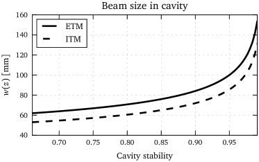
with $0\leq g\leq 1$ defining the stable region. Near-unstable cavities are of interest because they result in larger beam sizes on the cavity mirrors (see also figure 3) which reduces the coating thermal noise Vinet (2009), one of the limiting noise sources of the detector. One negative aspect of such near-unstable cavities is that the transverse optical mode separation frequency approaches zero as $g\rightarrow 0$ or $1$. The mode separation frequency determines the difference in resonance frequency of higher-order modes with respect to the fundamental mode. Thus with a lower separation frequency any defect in the cavity causing scattering into HOMs is suppressed less and can contaminate control signals for that cavity and couple extra noise into the GW detectors output . The optimal cavity design must be determined as a trade-off between these degrading effects and the reduction in coating thermal noise. This is a typical task where a numerical model can be employed to search the parameter space. In this case each point in that parameter space corresponds to a different beam size in the cavity which forces a re-computation of the scattering matrices on the mirrors. Thus the new algorithm described in this paper should yield a significant reduction in computing time.

In this section we briefly summarise the results from the simulations and in the following section we provide the details of setting up the model and give an analysis of the performance of the ROQ algorithm. We have implemented the ROQ integration in our open-source simulation tool Finesse and use the official input parameter files for the LIGO detectors ali . Below we show the preliminary investigation of the behaviour of a single Advanced LIGO like arm cavity with a finesse of 450, where the mirror maps for the mirrors ETM08 and ITM04 were applied to the high reflective (HR) surfaces. Note that we do not report the scientific results of the simulation task which will be published elsewhere. This example is representative for a class of modelling performed regularly for the LIGO commissioning and design and provides us with a concrete and quantitive setup to demonstrate the required steps to use the ROQ algorithm.

Figure 4: The Pound-Drever-Hall error signal for the LIGO cavity modelled in figure 2. A significant change in zero-crossing position and shape can be seen as the stability of the cavity is reduced ($g\rightarrow 1$).

Figure 5: Range of beam parameters needed to model a change in curvature from 0 m to 90 m at the ITM and the ETM. In order to utilise the ROQ to cover this parameter space, the empirical interpolant needs to be constructed using a training set made from kernels (6) densely covering this space.

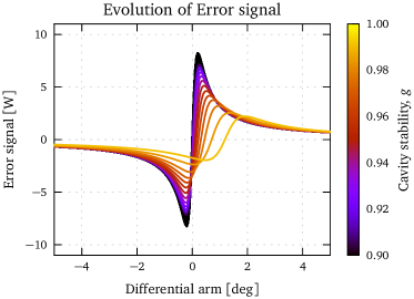
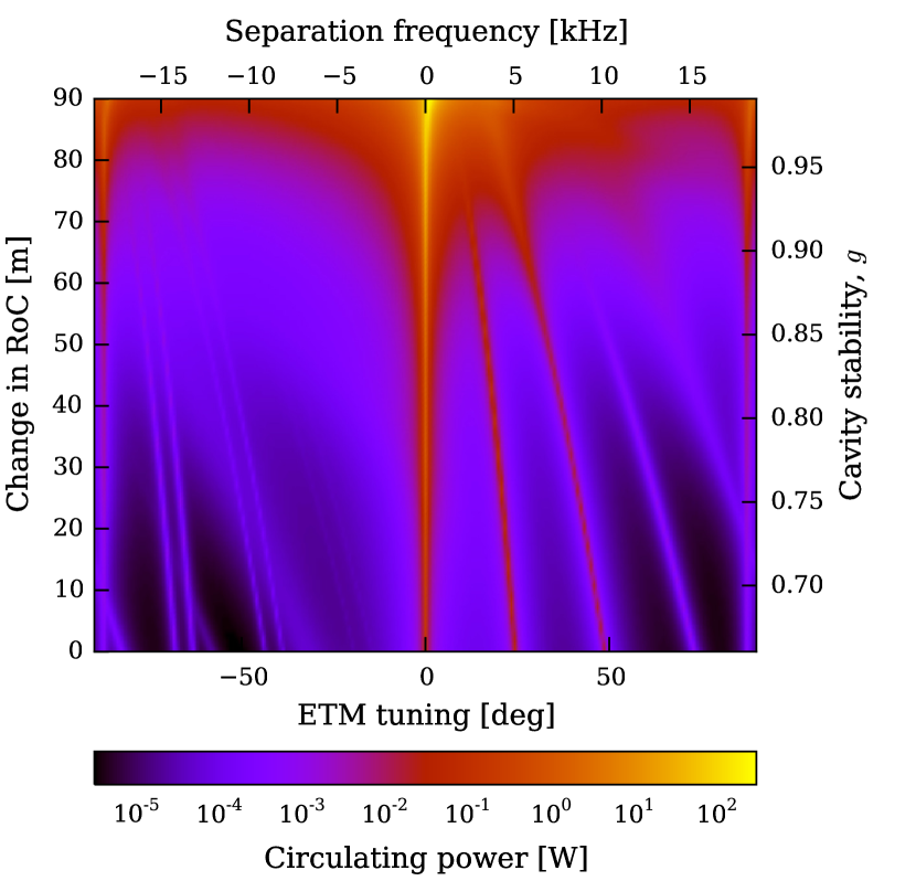
Modelling the LIGO cavity for differing stabilities involves varying the RoC of both the ITM and ETM. The resulting change in $w(z)$ at each surface means the scattering matrices will need to be recomputed for each state we choose. To view the HOM content in the cavity created by the scattering a cavity scan can be performed, displacing one of the cavity mirrors along the cavity axis on the order of the wavelength of the laser light, $\lambda=1064$ nm, to change the resonance condition of the cavity. We have performed the simulations using $\mathcal{O}=10$ with Newton-Cotes integration and our ROQ method. The results for cavity scans at different RoCs are shown in figure 2(a). The dominant mode is the fundamental TEM₀₀ whose resonance defines the zero tuning, the power in the TEM₀₀ mode has been removed from this plot to better show the lower power HOM content. For more stable cavities (at the bottom of the plot in figure 2(a)) the HOMs are well separated and not resonant at the same time as the TEM₀₀. As the RoC is increased, the stability is reduced and the HOMs can be seen to converge and eventually become resonant at a tuning of 0. At a stability of $g\approx 0.98$ the cavity mode begins to break down significantly and many modes become resonant. The effect of this on a sensing and control signal used for a Pound-Drever-Hall control system is shown in figure 4, where for increasingly unstable cavities the error signal becomes degraded, showing an offset to the nominal zero crossing, a reduced slope and overall asymmetry around the centre. The complete investigation into the feasibility of such cavities is beyond the scope of this paper, it includes amongst other issues the quantitative comparison of the control noise from the degradation of the control signals with the reduced thermal noise. The simulation task described above is sufficient to provide a test case for our ROQ method.

V Application and performance of new integration method

In this section we provide a detailed and complete recipe for setting up and using the ROQ for the LIGO example, using Finesse and Pykat, and discuss the performance, in terms of speed and accuracy, of our method. The description should be sufficient for the reader to implement our method for their own optical setup. In this section we include the costly “offline” procedure of building the empirical interpolant for completeness. As part of the ongoing code development of Finesse and Pykat we intend to pre-generate the empirical interpolants, suitable for a wide range of problems, so that the typical user should not need to run the costly offline building of the interpolant into their simulations.

V.1 Computing the ITM and ETM Empirical Interpolants

Firstly the range of beam parameters for the simulation must be determined. Once this is known a training set can be constructed and the empirical interpolant can be computed. The surface distortions that are of interest are those on the HR surfaces of a LIGO arm cavity mirror. We will require two EIs, one for the ITM HR surface and one for the ETM HR surface due to the differing beam parameters at each mirror. The beam parameter range that the training sets should span are determined by varying the radius of curvature of the ITM and ETM to include the range of cavity stabilities which we want to model. The beam parameter ranges are shown in figure 5. The required ranges for the ETM are $4.7\mathrm{m}<w_{0}<12.0\mathrm{mm}$ and $2.11\mathrm{km}<z<2.20\mathrm{km}$ and for the ITM $4.7\mathrm{mm}<w_{0}<12.0\mathrm{m}$ and $-1.88\mathrm{km}<z<-1.79\mathrm{km}$, up to a maximum optical mode order of $\mathcal{O}=20$, Netwon-Cotes degree of 6, $L=1199$. For this example we fix the maximum tolerable error of the empirical interpolant to $\epsilon=10^{-14}$.

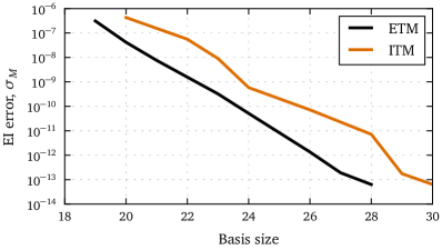
Using these ranges the method described in section III.1 can be used to produce the EIs. The offline computation of the basis can have significant computational cost. For very wide parameter ranges the memory required to store the training sets can quickly exceed that of typical machines. For the above parameters, with 100 sample points each in the $w_{0}$ and $z$ range, up to $\mathcal{O}=14$ and $\epsilon=10^{-14}$ approximately 7GB of memory was required. Running this method on machines with less memory is possible by storing the training set on a hard drive using a suitable data storage format such as HDF5 for access. Computation time of the empirical interpolant is then limited by the read and write times of the media. Using a MacBook pro 2012 model which contains a 2.7 GHz Intel core i7 with 8GB of RAM generating the ITM and ETM reduced basis and empirical interpolant takes $\approx 4$ hours each. The number of elements in the final reduced basis for the ITM and ETM were $N=30$ and $N=29$ respectively. In figure 8 the convergence of the empirical interpolant error with respect to the acceptable empirical interpolant error. One can see that the EI error converges exponentially as described in section III.4.

V.2 Producing the ROQ weights

Figure 6: Absolute and argument values of the ROQ weights (20) generated for each of the maps as shown in figure 1. Here the final quadrature rule can be visualized. The top plots show the absolute value: The size of the point is proportional to $|w|$ and the center of each point lies on a specific empirical interpolation node in the x-y plane $(X_{i},Y_{j})$ (c.f. (13) and (19)). The bottom plots show $\log_{10}(arg(w))$. The dashed line on each plot shows the mirror surface boundary; outside the boundary the mirror maps are equal to zero. We note that there are non-zero ROQ weights associated with points in the region where the mirror maps are zero. While this may be counter intuitive, it is a consequence of the fact that the empirical interpolant nodes lie within the full x-y plane and, that they are constructed without any knowledge of the mirror maps: the weights still receive no contribution from the region where $A(x,y)=0$ as this region does not contribute to the sum in (20). However, the ROQ uses information about the kernels (6) over the entire region, including where $A(x,y)=0$.

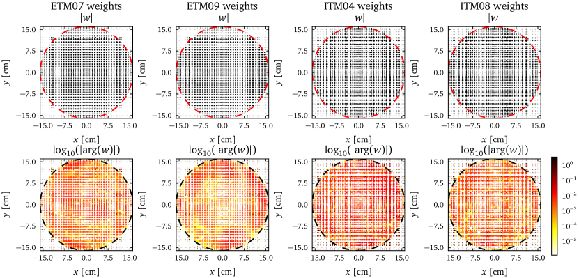
Once the empirical interpolant has been computed for both ITM and ETM HR surfaces the ROQ weights (20) can be computed by convoluting the mirror maps with the interpolant. The surface maps that we have chosen are the measured surface distortions of the (uncoated) test masses currently installed at the LIGO Livingston observatory, shown in figure 1. The maps contain $L\approx 1200$ samples and we can expect a theoretical speed-up of $L^{2}/N^{2}\approx 1200^{2}/30^{2}=1600$ from using ROQ over Newton-Cotes. These maps include an aperture, $\mathcal{A}$, and the variation in surface height in meters, $z(x,y)$. Thus to calculate the HOM scattering on reflection from one of these mirrors with (5) the distortion term is:

$$A(x,y)=\mathcal{A}(x,y)e^{2\mathrm{i}kz(x,y)}$$ (22)

where $\mathcal{A}(x,y)$ is 1 if $\sqrt{x^{2}+y^{2}}<0.16$m and 0 otherwise, and $k$ is the wavenumber of the incident optical field.

Using (22) with equation (20) (with a Newton-Cotes rule of the same degree the empirical interpolant was generated with) the ROQ weights can be computed for each map shown in figure 1. This computational cost is proportional to the number of elements in the EI, $M$, and the number of samples in the map, $L^{2}$. For the LIGO maps this takes $\approx 10$s on our 2012 MacBook Pro. The resulting ROQ rule for the maps can be visualised as shown in figure 6: the amplitude of the ROQ weights map out the aperture and the phase of the weights varies for different maps because of the different surface structure. The computation of these ROQ weights need only be performed once for each map, unless the range of beam parameters required for the empirical interpolant are changed.

(a) ROQ error for $\mathcal{O}_{max}=10$

(b) ROQ error for $\mathcal{O}_{max}=14$

(c) ROQ error for $\mathcal{O}_{max}=18$

Figure 7: Maximum relative error between the scattering matrices computed for the ETM07 surface map, with ROQ and using Newton-Cotes, for mode orders up to $\mathcal{O}_{max}=18$. The dashed white area represents the beam-parameter region over which training sets were generated. The subplots illustrates how using an ROQ built for a larger $\mathcal{O}_{max}$ scattering reduces the maximum error significantly. Also shown is that the ROQ is valid over a larger parameter range than what it was initially generated for, implying that the empirical interpolant can be used for extrapolation in a limited parameter region outside the initial range indicated by the white dashed box.

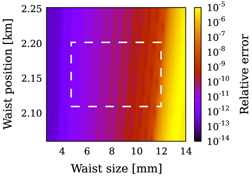
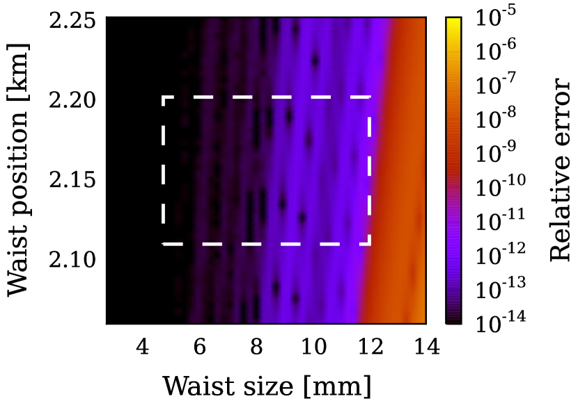
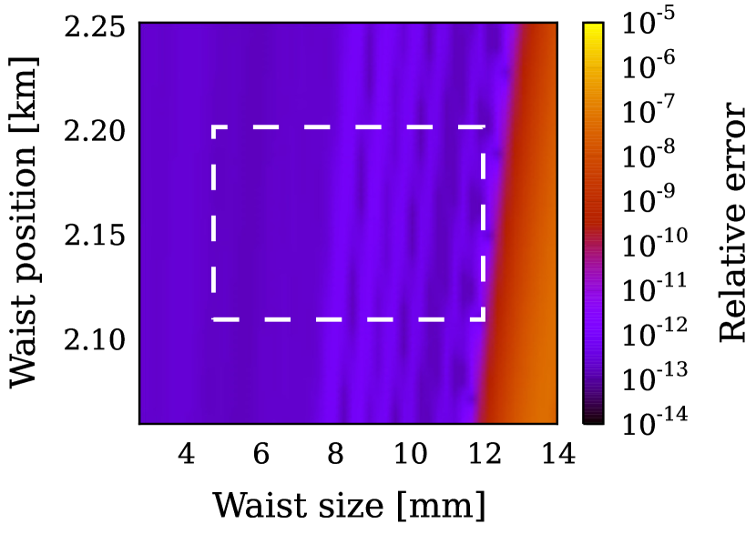
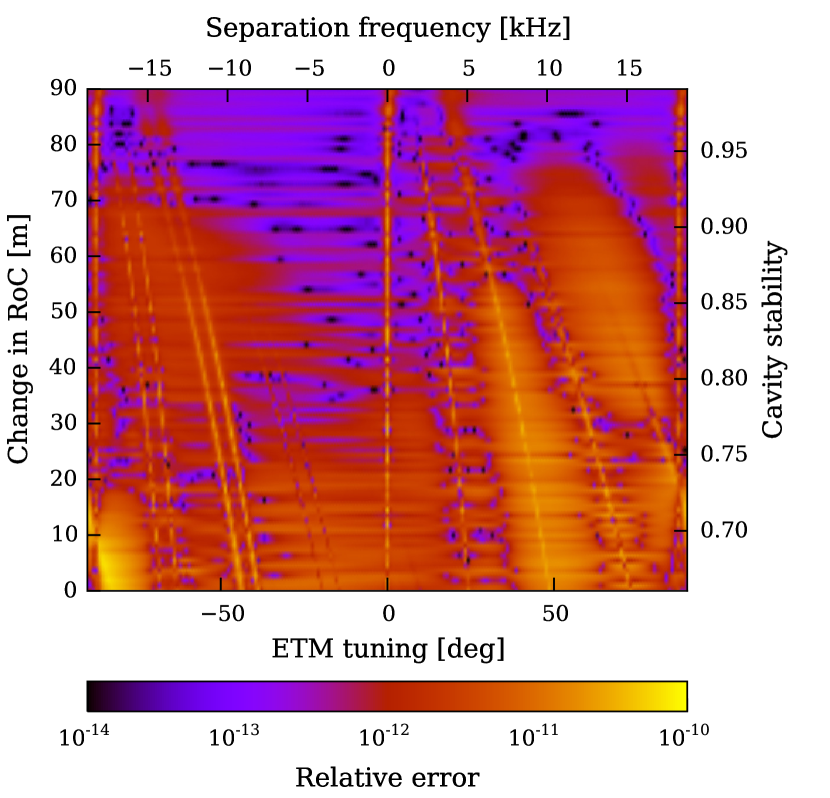
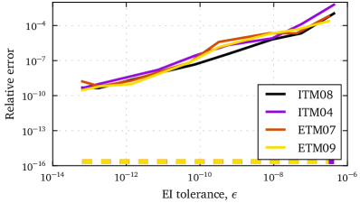
We verify that the process of generating the ROQ rule has worked correctly by computing the scattering matrices with ROQ and Newton-Cotes across the parameter space. We compute $\hat{k}(q;\mathrm{ETM07})$ with $\mathcal{O}_{max}=10$ using ROQ and then again using Newton-Cotes integration. Computing the relative error between each element of these two matrices the maximum error can be taken for $q$ values spanning the requested $q$ parameter range. Figure 9 shows how the final error of the EI, $\sigma_{M}$, propagates into an error in the scattering matrix. This shows the maximum (solid line) and minimum (dashed line) errors for any element in the scattering matrix between the two methods. From this it can be seen that building a more accurate empirical interpolant results in smaller maximum errors in the scattering matrix. Now, using the most accurate reduced basis the maximum relative error is shown in figure 7 over the $q$ space, where the white dashed box shows the boundaries of the parameters in the training set. Overall the method successfully computed a ROQ rule that accurately reproduced the Newton-Cotes results for scattering up to $\mathcal{O}=10$. In should be notes that the largest errors, e.g. as seen in figure 9, do not represent the full parameter space but occur only at smallest $z$ and largest $w_{0}$. It was also found that building a basis including a higher maximum HOM, for example basis of order 14 for scattering computations up to order 10, significantly improved the accuracy of the ROQ. Using an reduced basis constructed for order 14 rather than order 10 only increased the number of elements in the basis by 2, thus not significantly degrading any speed improvements. It can also be seen in figure 7 that ROQ extrapolates beyond the originally requested $q$ parameter space and does not instantly fail for evaluations outside of it. A gradual decrease in the accuracy can be seen when using larger $w_{0}$ values.

Figure 8: EI error as a function of the number of basis elements selected by the greedy algorithm (Alg. 1) for the example described in section V.1. As expected from the error analysis in section III.4, the empirical interpolant error displays exponential convergence with the basis size.

Figure 9: Relative error in the scattering matrices computed using the ROQ and Newton-Cotes integration (with $\mathcal{O}_{max}=10$) as a function of the empirical interpolant tolerance $\epsilon$. The empirical interpolant was built for maximum coupling $\mathcal{O}_{max}=14$. The error is the minimum (dashed lines) and maximum (solid lines) over the parameter space with which the empirical interpolant was built for, thus represents the worst and best case scenarios. The largest errors are independent of the map data and occur on couplings coefficients which couple the higher order modes included in the empirical interpolant.

V.3 Performance

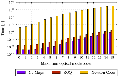
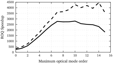
The time taken to run these Finesse simulations as $\mathcal{O}$ is increased is shown in figure 10 demonstrating how much more efficient it is to use ROQ over Newton-Cotes for the computation of scattering matrices. We also show for reference the computation time when no scattering from surface maps is included to give the base time it takes to run the rest of the Finesse simulation. The overall speed-up achieved can be seen in figure 11, reaching $\approx 2700$ times faster to run the entire simulation at $\mathcal{O}=10$. The overall speed-up then begins to drop slightly as the base time taken to run the rest of Finesse becomes larger. The dashed line in figure 11 shows the speed-up if this base time is removed, again showing an impressive speed-up peaking at 4000 times faster.

Figure 10: Time taken to run Finesse to model the steady state optical fields in an LIGO cavity with surface maps on both the ITM and ETM HR surfaces. The timing of running the entirety of Finesse is used—rather than just the core method—because there are additional speed improvements from having to read and handle significantly less data points, from the $L\times L$ maps down to $M\times M$ ROQ weights. Smaller data fits into processor caches better and also reduces disk read times. This plot compares a single computation of the scattering matrices with ROQ (19) and Newton-Cotes. The case with no maps used is also shown to illustrate how much time is spent in Finesse doing calculations not involving maps, which now becomes the dominant computational cost when using ROQ. A significant improvement is also found for order zero where only one scattering integral need be calculated; this is partly time saved from having to read larger data from the disk and manipulating it in memory. The preprocessing is unavoidable as the Finesse can except many different types of map, thus it cannot be optimised at runtime until it know what it is dealing with. ROQ helps here as it removes this preprocessing step so it need only happen once. The ROQ preprocessing happens during the computing of the ROQ weights (20). This is a one time cost for each map for a particular EI donqe outside of Finesse, thus isn’t included in this timing. The computational cost of this is on the order of 5s for each map for the reduced basis used in this example.

Figure 11: The speed-up achieved using ROQ compared to Netwon-Cotes as a function of mode order using the timing values in figure 10. The dashed line shows the speed-up if the time for initialisation and post-processing is subtracted from both times for Newton-Cotes and ROQ. This demonstrates the improvements just for the computational cost relating to map scattering calculations. Simulations that have a larger computational cost relating to features not related to scattering will show a smaller speed-up. For example, the simulations results shown in figure 2 have a total simulation speed-up of $\approx 80$ but the scattering calculation was reduced from $\approx 20.5\,\text{Hours}\rightarrow 30\,\text{s}$.

Using ROQ enables us to perform such modelling tasks with a far greater efficiency. Running the model to compute the output seen in figure 2(a) required computing 100 different scattering matrices for the various changes in RoC. This took 20.5 hours to compute with Newton-Cotes and 18 minutes with ROQ . The difference in the final result between ROQ and Newton-Cotes is shown in terms of relative error in figure 2(b). We have prepared the ROQ input for this example such that the error is significantly lower than 1 ppm (relative error of $10^{-6}$) thereby showing that ROQ can be both much faster and still sufficiently accurate.

VI Conclusion

Numerical modelling of optical systems plays a vital role for the design and commissioning of precision interferometers. The typical use of the simulation software in this area requires rapid iterations of many simulation runs and manual fine tuning as modelling progresses, which is not well suited for large computer clusters. The scope of current investigations is often limited by the required computation time and thus the development of fast and flexible tools is a priority. Current problems in precision interferometers, such as LIGO, involve the investigation of laser beam shape distortions and their effect on the interferometer signal. Frequency-domain simulations using Gaussian modes to describe the beam properties have emerged as fast and flexible tools. However, the computation of the scattering matrix for mirror surface distortions—effectively an overlap integral of measured surface data with Hermite-Gauss modes—has shown to be a limiting factor in improving the computational speed of such tools. A significant reduction in computational time of current numerical tools is required for more efficient in-depth modelling of interferometers including more realistic features such as clipping, optical defects, thermal distortions and parametric instabilities.

In this work we have demonstrated how the empirical interpolation method can be used to generate an optimised quadrature rule for paraxial optical scattering calculations, known as a reduced order quadrature. Our method removes the prohibitive computational cost of computing the scattering by speeding up the calculation of the steady state optical fields in a LIGO arm cavity by up to a factor of $\leavevmode\nobreak\ 2750$ times, reducing simulation times from days to minutes. Using an exemplary simulation task of near-unstable arm cavities for the LIGO interferometers we have demonstrated that our method is both accurate and fast for a typical modelling scenario where imperfections in the interferometer have a significant impact on optical performance. We have provided a complete recipe to recreate and use the new algorithm and provide an open source implementation in our general-purpose simulation software Finesse. Importantly, the reduced order quadrature integration method is generic and can be applied to any optical scattering problem for any surface distortion data.

VII Acknowledgements

We would like to thank GariLynn Billingsley for providing the Advanced LIGO mirror surface maps and for advice and support on using them. We would also like to thank Peter Deiner, Scott Field and Chad Galley for useful discussions and encouragement throughout this project. Some of the computations were carried out using the high performance computing resources provided by Louisiana State University (http://www.hpc.lsu.edu) and the Extreme Science and Engineering Discovery Environment (XSEDE) Towns et al. (2014), which is supported by National Science Foundation grant number ACI-1053575. This work has been supported by the Science and Technology Facilities Council and the U.S. National Science Foundation under cooperative agreement NSF-PHY-0757058. This document has been assigned the LIGO Laboratory document number LIGO-P1500128-v1.

References

- Grote and the LIGO Scientific Collaboration (2008) Hartmut Grote and the LIGO Scientific Collaboration. The status of GEO 600. Classical and Quantum Gravity, 25(11):114043 (9pp), 2008. URL http://stacks.iop.org/0264-9381/25/114043.
- Sigg and the LIGO Scientific Collaboration (2008) Daniel Sigg and the LIGO Scientific Collaboration. Status of the LIGO detectors. Classical and Quantum Gravity, 25(11):114041, 2008. URL http://stacks.iop.org/0264-9381/25/i=11/a=114041.
- Acernese et al. (2008) F Acernese et al. Virgo status. Classical and Quantum Gravity, 25(18):184001 (9pp), 2008. URL http://stacks.iop.org/0264-9381/25/184001.
- Takahashi and the TAMA Collaboration (2004) Ryutaro Takahashi and the TAMA Collaboration. Status of TAMA300. Classical and Quantum Gravity, 21(5):S403, 2004. URL http://stacks.iop.org/0264-9381/21/i=5/a=004.
- Aasi et al. (2015) J Aasi et al. Advanced LIGO. Classical and Quantum Gravity, 32(7):074001, 2015. URL http://stacks.iop.org/0264-9381/32/i=7/a=074001.
- Acernese et al. (2015) F Acernese et al. Advanced Virgo: a second-generation interferometric gravitational wave detector. Classical and Quantum Gravity, 32(2):024001, 2015. URL http://stacks.iop.org/0264-9381/32/i=2/a=024001.
- STAIC (2000) STAIC. Software tools for advanced interferometer configurations. http://www.phys.ufl.edu/LIGO/LIGO/STAIC.html, 2000. Accessed: 2014-11-18.
- GWIC (2013) GWIC. Numerical modelling tools for gravitational wave detectors. https://gwic.ligo.org/simulations, 2013. Accessed: 2014-11-18.
- Caron et al. (1999) B. Caron et al. SIESTA, a time domain, general purpose simulation program for the VIRGO experiment. Astropart.Phys., 10:369–386, 1999. doi: 10.1016/S0927-6505(98)00059-0.
- Yamamoto et al. (2000) H Yamamoto et al. End to end simulation program for gravitational-wave detectors. In Seiji Kawamura and Norikatsu Mio, editors, Graviational Wave Detection II, number 32 in Frontier Science Series. Universal Academy Press, 2000.
- Vinet (2009) Jean-Yves Vinet. On special optical modes and thermal issues in advanced gravitational wave interferometric detectors. Living Reviews in Relativity, 12(5), 2009. URL http://www.livingreviews.org/lrr-2009-5.
- Vinet et al. (1992) J.-Y. Vinet, P. Hello, C. N. Man, and A. Brillet. A high accuracy method for the simulation of non-ideal optical cavities. Journal de Physique I, 2:1287–1303, July 1992. doi: 10.1051/jp1:1992211.
- Beausoleil et al. (2003) Raymond G. Beausoleil et al. Model of thermal wave-front distortion in interferometric gravitational-wave detectors. i. thermal focusing. J. Opt. Soc. Am. B, 20(6):1247–1268, Jun 2003. doi: 10.1364/JOSAB.20.001247. URL http://josab.osa.org/abstract.cfm?URI=josab-20-6-1247.
- science team (2010) ET science team. Einstein gravitational wave telescope conceptual design study. Technical Report ET-0106C-10, 2010, https://tds.ego-gw.it/itf/tds/.
- R et al. (2008) Schibli T R et al. Optical frequency comb with submillihertz linewidth and more than 10 w average power. Nature Photonics, 2:355 – 359, 2008.
- Dickerson et al. (2013) Susannah M. Dickerson, Jason M. Hogan, Alex Sugarbaker, David M. S. Johnson, and Mark A. Kasevich. Multiaxis inertial sensing with long-time point source atom interferometry. Phys. Rev. Lett., 111:083001, Aug 2013. doi: 10.1103/PhysRevLett.111.083001.
- Freise and Strain (2010) A. Freise and K. Strain. Interferometer Techniques for Gravitational-Wave Detection. Living Reviews in Relativity, 13:1–+, February 2010. URL http://relativity.livingreviews.org/Articles/lrr-010-1/2.
- Bond et al. (2013) Charlotte Bond, Paul Fulda, Daniel Brown, and Andreas Freise. Investigation of beam clipping in the power recycling cavity of Advanced LIGO using Finesse. Technical Report LIGO Document T1300954, Nov 2013.
- Freise et al. (2004) A Freise et al. Frequency-domain interferometer simulation with higher-order spatial modes. Classical and Quantum Gravity, 21(5):S1067–S1074, 2004. URL http://stacks.iop.org/0264-9381/21/S1067. The program is available at http://www.gwoptics.org/finesse.
- (20) Finesse input files for Advanced LIGO. https://dcc.ligo.org/LIGO-L1300231. Accessed: 2015-07-13.
- Antil et al. (2013) Harbir Antil, ScottE. Field, Frank Herrmann, RicardoH. Nochetto, and Manuel Tiglio. Two-step greedy algorithm for reduced order quadratures. Journal of Scientific Computing, 57(3):604–637, 2013. ISSN 0885-7474. doi: 10.1007/s10915-013-9722-z. URL http://dx.doi.org/10.1007/s10915-013-9722-z.
- Canizares et al. (2015) Priscilla Canizares et al. Accelerated gravitational wave parameter estimation with reduced order modeling. Phys. Rev. Lett., 114:071104, Feb 2015. doi: 10.1103/PhysRevLett.114.071104. URL http://link.aps.org/doi/10.1103/PhysRevLett.114.071104.
- Maday et al. (2009) Y. Maday, N. C. Nguyen, A. T. Patera, and S. H. Pau. A general multipurpose interpolation procedure: the magic points. Communications on Pure and Applied Analysis, 8:383–404, 2009. doi: 10.3934/cpaa.2009.8.383.
- Kogelnik (1965) Herwig Kogelnik. On the propagation of Gaussian beams of light through lenslike media including those with a loss or gain variation. Appl. Opt., 4(12):1562–1569, 1965. URL http://ao.osa.org/abstract.cfm?URI=ao-4-12-1562.
- (25) G. Billingsley. LIGO core optics reference page. https://galaxy.ligo.caltech.edu/optics/. Accessed: 2015-07-13.
- Bond (2014) Charlotte Zoë Bond. How to stay in shape: overcoming beam and mirror distortions in advanced gravitational wave interferometers. July 2014. URL http://etheses.bham.ac.uk/5223/.
- Bayer-Helms (1984) F. Bayer-Helms. Coupling coefficients of an incident wave and the modes of spherical optical resonator in the case of mismatching and misalignment. Appl. Opt., 23:1369–1380, May 1984.
- Vinet and the Virgo Collaboration (2001) J. Y. Vinet and the Virgo Collaboration. The Virgo Book of Physics: Optics and Related Topics. Virgo, 2001. URL http://wwwcascina.virgo.infn.it/vpb/.
- Ralston and Rabinowitz (2001) A. Ralston and P. Rabinowitz. A First Course in Numerical Analysis. Dover books on mathematics. Dover Publications, 2001. ISBN 9780486414546. URL https://books.google.co.uk/books?id=czHV-1bEFl0C.
- Barrault et al. (2004) Maxime Barrault, Yvon Maday, Ngoc Cuong Nguyen, and Anthony T. Patera. An ‘empirical interpolation’ method: application to efficient reduced-basis discretization of partial differential equations. Comptes Rendus Mathematique, 339(9):667 – 672, 2004. ISSN 1631-073X. doi: http://dx.doi.org/10.1016/j.crma.2004.08.006. URL http://www.sciencedirect.com/science/article/pii/S1631073X04004248.
- Hesthaven et al. (2014) Jan S. Hesthaven, Benjamin Stamm, and Shun Zhang. Efficient greedy algorithms for high-dimensional parameter spaces with applications to empirical interpolation and reduced basis methods. ESAIM: Mathematical Modelling and Numerical Analysis, 48:259–283, 1 2014. ISSN 1290-3841. doi: 10.1051/m2an/2013100. URL http://www.esaim-m2an.org/action/article_S0764583X13001003.
- Gunzburger et al. (2007) Max D. Gunzburger, Janet S. Peterson, and John N. Shadid. Reduced-order modeling of time-dependent {PDEs} with multiple parameters in the boundary data. Computer Methods in Applied Mechanics and Engineering, 196(4–6):1030 – 1047, 2007. ISSN 0045-7825. doi: http://dx.doi.org/10.1016/j.cma.2006.08.004. URL http://www.sciencedirect.com/science/article/pii/S0045782506002337.
- Kirk et al. (2006) B. S. Kirk, J. W. Peterson, R. H. Stogner, and G. F. Carey. libMesh: A C++ Library for Parallel Adaptive Mesh Refinement/Coarsening Simulations. Engineering with Computers, 22(3–4):237–254, 2006.
- Press et al. (2007) William H. Press, Saul A. Teukolsky, William T. Vetterling, and Brian P. Flannery. Numerical Recipes 3rd Edition: The Art of Scientific Computing. Cambridge University Press, New York, NY, USA, 3 edition, 2007. ISBN 0521880688, 9780521880688.
- (35) Kendall Atkinson. An Introduction to Numerical Analysis. Wiley, 2 edition. ISBN 0471624896.
- Aanonsen (2009) Tor Øvstedal Aanonsen. Empirical interpolation with application to reduced basis approximations. 2009.
- Towns et al. (2014) John Towns et al. Xsede: Accelerating scientific discovery. Computing in Science and Engineering, 16(5):62–74, 2014. ISSN 1521-9615. doi: http://doi.ieeecomputersociety.org/10.1109/MCSE.2014.80.