1.4cm1.3cm0.3cm0.8cm
Fisher Information and entanglement of non-Gaussian spin states
Entanglement is the key quantum resource for improving measurement sensitivity beyond classical limits. However, the production of entanglement in mesoscopic atomic systems has been limited to squeezed states, described by Gaussian statistics. Here we report on the creation and characterization of non-Gaussian many-body entangled states. We develop a general method to extract the Fisher information, which reveals that the quantum dynamics of a classically unstable system creates quantum states that are not spin squeezed but nevertheless entangled. The extracted Fisher information quantifies metrologically useful entanglement which we confirm by Bayesian phase estimation with sub shot-noise sensitivity. These methods are scalable to large particle numbers and applicable directly to other quantum systems.
Multiparticle entangled states are the key ingredients for advanced quantum technologies NielsenBOOK . Various types have been achieved in experimental settings ranging from ion traps BlattNATURE2008 , photonic systems PanRMP2012 and solid state circuits VlastakisSCIENCE2013 to Bose-Einstein condensates. For the latter, squeezed states SorensenNATURE2001 ; WinelandPRA1994 have been generated EsteveNATURE2008 ; GrossNATURE2010 ; RiedelNATURE2010 ; ChapmanNATPHYS2012 ; LueckeSCIENCE2011 ; BerradaNATCOMM2013 and a rich class of entangled non-Gaussian states is predicted to be obtainable PezzePRL2009 including maximally entangled Schrödinger cat states MicheliPRA2003 ; CiracPRA1998 . The production of these fragile states in large systems remains a challenge and efficient methods for characterization are necessary because full state reconstruction becomes intractable. Here, we generate a class of non-Gaussian many-particle entangled states and reveal their quantum properties by studying the distinguishability of experimental probability distributions.
A measure of the distinguishability with respect to small phase changes of the state is provided by the Fisher information Fisher1925 . It is related to the highest attainable interferometric phase sensitivity by the Cramer-Rao bound HelstromBOOK . This limit follows from general statistical arguments for a measurement device with fluctuating output SuppInfo . The Fisher information is limited by quantum fluctuations of the input state as well as the performance of the device. Even in the absence of technical noise, the Fisher information of a classical input state is because of the intrinsic granularity of independent particles which translates into the shot-noise limit for phase estimation. This classical bound can be surpassed with a reduction of the input fluctuations by introducing entanglement between the particles SorensenNATURE2001 . These states, known as squeezed states, are fully characterized by mean and variance of the observable and already employed in precision measurements SchnabelNatComm2010 ; SewellPRL2012 ; OckeloenPRL2013 . In contrast, non-Gaussian quantum states can have increased fluctuations of the observable but nevertheless allow surpassing shot-noise limited performance. A textbook example is the Schrödinger cat state characterized by macroscopic fluctuations but achieving the best interferometric performance allowed by quantum mechanics, i.e. at the fundamental Heisenberg limit GiovannettiPRL2006 . In general, the class of states that are entangled and useful for sub shot-noise phase estimation is identified by the Fisher information criterion PezzePRL2009 . Exploiting these resources requires probabilistic methods for phase estimation such as maximum likelihood or Bayesian analysis KrischekPRL2011 which go beyond standard evaluation of averages.
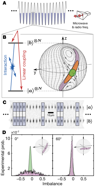
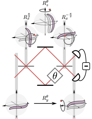
A paradigm physical process that exhibits the transition from Gaussian to non-Gaussian states is the time evolution of a quantum state initially prepared at an unstable classical fixed point. Our experimental system is an array of interacting binary Bose-Einstein condensates of 87Rb with additional linear coupling of the two internal states (see Fig. 1A–C), which allows for the controlled realization of such unstable fixed point dynamics ZiboldPRL2010 . The linear coupling, realized with microwave and radio frequency magnetic fields, also permits precise rotations for initial state preparation and final state manipulation before read-out (see Fig. 1B,D). For a coherent state initially centered on the unstable fixed point, the quantum dynamics leads to spin squeezed states for short evolution times that subsequently transform into non-Gaussian states on an experimentally feasible time scale MicheliPRA2003 (see Fig. 1B).
For the characterization of non-Gaussian states, higher moments, or even the full probability distributions, have to be accessed experimentally. For this, the setup GrossNATURE2010 has been extended to realize up to 35 individual condensates in a single experiment, which permits the acquisition of sufficient statistics in a narrow window of for the final atom number. The populations of the atomic states and are destructively detected for each individual condensate by state-selective absorption imaging with high spatial resolution (Fig. 1C) Muessel2013 . By repeating the experiment (typically many thousands of times), we measure the experimental probability distributions of the population imbalance along defined directions by applying the corresponding spin rotation before detection. The analysis window for is adjusted according to the independently determined time scale of atom loss SuppInfo to follow the time evolution starting with . Figure 1D shows examples of observed distributions for two different orientations and an evolution time of 25 ms; the distributions are consistent with the theoretically expected structure of the state (see Fig. 1B).
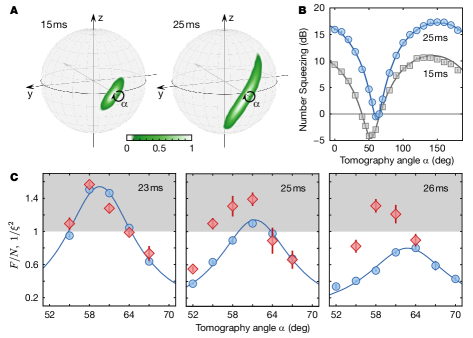
Detailed insight can be gained by repeating this measurement for various angles (here in steps of 10 degrees) allowing for the maximum-likelihood reconstruction of the density matrix in the symmetric subspace SuppInfo . Figure 2A shows the tomography results obtained from 32,500 experimental realizations confirming qualitatively the expected behavior – at short evolution times the state has a squeezed shape whereas at later times the characteristic bending dynamics appears as expected from the presence of the two stable fixed points above and below the equator.
Analyzing the variance of for the same data as a function of the tomography angle (Fig. 2B) shows that the time evolution leads to suppressed fluctuations at 15 ms. Extracting the spin squeezing parameter SuppInfo we find the minimum dB below the standard quantum limit which demonstrates entanglement SorensenNATURE2001 . We note that, for all results reported here, the photon shot-noise of the absorption imaging of atoms is not subtracted. For longer time evolution the bending dynamics leads to increased fluctuations in all directions i.e. tomography angles. After 25 ms spin squeezing is lost and we find dB. However as shown in Fig. 2C, experimental extraction of the Fisher information (detailed below) reveals that useful entanglement is still present although spin squeezing is vanishing, i.e. PezzePRL2009 . At 26 ms, spin squeezing is completely lost whereas the Fisher information still indicates the presence of quantum resources (). In the Gaussian regime up to 23 ms, we observe that Fisher information and the inverse spin squeezing agree as expected as these states are fully characterized by their variance.
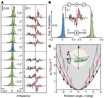
Our method for extraction of the Fisher information circumvents the experimentally intractable full reconstruction of the density matrix and is based on a specific set of experimental probability distributions after small rotations of the quantum state. As an example, in Fig. 3A we show distributions for the state created at 26 ms and the optimal tomography angle of 58 degrees (see Fig. 2C) after small rotations about the axis (see Fig. 3C inset), which feature a pronounced peak and long tails characteristic for the bent state. The main effect of the small rotation is a continuous shift of the distribution towards increasing imbalance for larger angles .
The analysis for extraction of the Fisher information builds on the statistical distance WoottersPRD1981 ; BraunsteinPRL1994 of these distribution functions. We use a Euclidean distance in the space of probability amplitudes known as Hellinger distance SuppInfo , defined as
| (1) |
According to the definition, we take the square root of the experimental probability distributions at finite and and calculate the difference for each bin (red histograms in Fig. 3A,B). Summing the squares of the differences provides the squared Hellinger distance . Figure 3C shows as a function of for three different evolution times and the respective optimal tomography angles. A resampling method SuppInfo is used to extract error bars and reduce the statistical bias. The observed quadratic behavior is expected from the Taylor expansion
| (2) |
which reveals the close connection between Hellinger distance and Fisher information; this relationship is used to extract from the curvature of . The gray shaded area in Fig. 3C indicates the region that is not accessible to separable states; for them, the Fisher information is limited to , resulting in a curvature smaller than . For the initially prepared state we find a Fisher information of , which is expected for a separable state. For a subsequent evolution of 26 ms the measured Hellinger distances lie in the regime of non-separability. This reveals entanglement in a regime where no spin squeezing is present. For the intermediate evolution time of 15 ms we extract a Fisher information , which confirms entanglement in the Gaussian spin squeezed state. For obtaining the systematic study of Fig. 2C, this procedure is performed at a given evolution time for different tomography angles. The reported values for the Fisher information are limited by experimental imperfections, detection noise and atom loss which especially affect the fragile non-Gaussian states. For the ideal time evolution, monotonically increasing Fisher information is expected, whereas the available spin squeezing is limited to (-12.6 dB). The ideal theoretical model prediction is (-19.5 dB) for the evolution time when spin squeezing vanishes SuppInfo .
There is a direct connection between Fisher information and sensitivity in parameter estimation. In an interferometric context, high sensitivity, indicated by a large value of , means fast change of the output distribution with the phase , i.e. high statistical speed with respect to the parameter change. For the quantum state at 25 ms the enhanced Fisher information reveals quantum resources beyond the standard quantum limit in a range of tomography angles. No squeezing is detected for the optimum at 58 degrees, which implies that these resources can only be exploited with the knowledge of more details of the distribution functions. In Fig. 4A we show explicitly through mean and variance analysis that averaging of the observable does not surpass shot-noise limited performance for rotations about the axis (corresponding for example to a phase shift inside a Ramsey interferometer SuppInfo ).
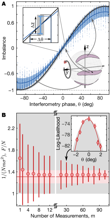
However, the resource can be harnessed with model independent Bayesian estimation using the experimental probability distributions . For this, we use an independent data set taken with the setting (, ) and 25 ms of evolution time, which we divide into sequences each containing realizations. To obtain realistic measurement conditions, we discard the previous knowledge on the true value of the phase (Bayesian estimation with flat prior SuppInfo ). For each distribution we calculate the likelihood
| (3) |
which corresponds to the conditional probability to obtain the sequence if the phase setting had been . For sufficiently large we expect a Gaussian distribution centered at with the Bayesian phase uncertainty SuppInfo . Thus, can be extracted from a quadratic fit to (see Fig. 4B inset). We find a fast convergence of to the expected value (Cramer-Rao bound for measurements) already for (Fig. 4B). This explicitly shows phase uncertainty below the standard quantum limit in agreement with the Fisher information obtained from the Hellinger distance method described above.
In conclusion, we have developed a method based on the statistical distance of experimental probability distributions to extract the Fisher information, which was previously unattainable in systems of large particle number. We demonstrate this on a novel class of collective states in binary Bose-Einstein condensates generated in the vicinity of a classically unstable point. The experimental value of the Fisher information serves to verify entanglement in the absence of spin squeezing and quantifies the quantum resource for improved phase estimation. We confirm this by characterizing the sensitivity of a Ramsey interferometer and find enhanced performance in agreement with the extracted Fisher information. The presented method does not depend on the special shape of the probability distributions and is not limited to small particle numbers. It is therefore broadly applicable to the efficient characterization of highly entangled states, relevant for further improvement of atom interferometers AppelPNAS2009 ; GrossNATURE2010 ; LerouxPRL2010 ; LueckeSCIENCE2011 ; ChenPRL2011 ; SewellPRL2012 ; BerradaNATCOMM2013 ; OckeloenPRL2013 toward the ultimate Heisenberg limit GiovannettiPRL2006 . More generally, it can be applied to any phenomenon characterizable by the distinguishability of quantum states, as in quantum phase transitions Zanardi , quantum Zeno dynamics SmerziPRL2012 and quantum information protocols NielsenBOOK .
Acknowledgements We thank J. Tomkovič, E. Nicklas and I. Stroescu for technical help and discussions. This work was supported by the Forschergruppe FOR760, the Deutsche Forschungsgemeinschaft, the Heidelberg Center for Quantum Dynamics and the European Commission small or medium-scale focused research project QIBEC (Quantum Interferometry with Bose-Einstein condensates, Contract Nr. 284584). W.M. acknowledges support by the Studienstiftung des deutschen Volkes. D.B.H. acknowledges support from the Alexander von Humboldt foundation. L.P. acknowledges financial support by MIUR through FIRB Project No. RBFR08H058. QSTAR is the MPQ, LENS, IIT, UniFi Joint Center for Quantum Science and Technology in Arcetri.
Published in Science 345, 424-427 (2014)
doi: 10.1126/science.1250147
PDF also available via
http://www.matterwave.de/publications
References
- (1) M. A. Nielsen, I. L. Chuang, Quantum Computation and Quantum Information (Cambridge, 2000).
- (2) R. Blatt, D. Wineland, Entangled states of trapped atomic ions. Nature 453, 1008–1015 (2008).
- (3) J.-W. Pan et al., Multiphoton entanglement and interferometry. Rev. Mod. Phys. 84, 777–838 (2012).
- (4) B. Vlastakis et al., Deterministically Encoding Quantum Information Using 100-Photon Schrödinger Cat States. Science 342, 607–610 (2013).
- (5) A. Sørensen, L.-M. Duan, J. I. Cirac, P. Zoller, Many-particle entanglement with Bose-Einstein condensates. Nature 409, 63–66 (2001).
- (6) D. J. Wineland, J. J. Bollinger, W. M. Itano, D. J. Heinzen, Squeezed atomic states and projection noise in spectroscopy. Phys. Rev. A 50, 67 (1994).
- (7) J. Estève, C. Gross, A. Weller, S. Giovanazzi, M. K. Oberthaler, Squeezing and entanglement in a Bose-Einstein condensate. Nature 455, 1216–1219 (2008).
- (8) C. Gross, T. Zibold, E. Nicklas, J. Estève, M. K. Oberthaler, Nonlinear atom interferometer surpasses classical precision limit. Nature 464, 1165–1169 (2010).
- (9) M. F. Riedel et al., Atom-chip-based generation of entanglement for quantum metrology. Nature 464, 1170–1173 (2010).
- (10) C. D. Hamley, C. S. Gerving, T. M. Hoang, E. M. Bookjans, M. S. Chapman, Spin-nematic squeezed vacuum in a quantum gas. Nat. Phys. 8, 305–308 (2012).
- (11) M. S. Berrada et al., Integrated Mach-Zehnder interferometer for Bose-Einstein condensates. Nat. Commun. 4:2077, doi: 10.1038/ncomms3077 (2013).
- (12) B. Lücke et al., Twin Matter Waves for Interferometry Beyond the Classical Limit. Science 334, 773–776 (2011).
- (13) L. Pezzé, A. Smerzi, Entanglement, Nonlinear Dynamics, and the Heisenberg Limit. Phys. Rev. Lett. 102, 100401 (2009).
- (14) A. Micheli, D. Jaksch, J. I. Cirac, P. Zoller, Many-particle entanglement in two-component Bose-Einstein condensates. Phys. Rev. A 67, 013607 (2003).
- (15) J. I. Cirac, M. Lewenstein, K. Mølmer, P. Zoller, Quantum superposition states of Bose-Einstein condensates. Phys. Rev. A 57, 1208–1218 (1998).
- (16) R. A. Fisher, Theory of Statistical Estimation. Proc. Cambridge Phil. Soc. 22, 700–725 (1925).
- (17) C. W. Helstrom, Quantum Detection and Estimation Theory (Academic Press, New York, 1976).
- (18) See supplementary materials.
- (19) R. J. Sewell et al., Magnetic Sensitivity Beyond the Projection Noise Limit by Spin Squeezing. Phys. Rev. Lett. 109, 253605 (2012).
- (20) C. F. Ockeloen, R. Schmied, M. F. Riedel, P. Treutlein, Quantum Metrology with a Scanning Probe Atom Interferometer. Phys. Rev. Lett. 111, 143001 (2013).
- (21) R. Schnabel, N. Mavalvala, D. E. McClelland, P. K. Lam, Quantum metrology for gravitational wave astronomy. Nat. Commun. 1:121, doi: 10.1038/ncomms1122 (2010).
- (22) V. Giovannetti, S. Lloyd, L. Maccone, Quantum Metrology. Phys. Rev. Lett. 96, 010401 (2006).
- (23) R. Krischek et al., Useful Multiparticle Entanglement and Sub-Shot-Noise Sensitivity in Experimental Phase Estimation. Phys. Rev. Lett. 107, 080504 (2011).
- (24) T. Zibold, E. Nicklas, C. Gross, M. K. Oberthaler, Classical Bifurcation at the Transition from Rabi to Josephson Dynamics. Phys. Rev. Lett. 105, 204101 (2010).
- (25) W. Muessel et al., Optimized absorption imaging of mesoscopic atomic clouds. Appl. Phys. B. 113, 69 (2013).
- (26) W. K. Wootters, Statistical distance and Hilbert space. Phys. Rev. D 23, 357–362 (1981).
- (27) S. L. Braunstein, C. M. Caves, Statistical Distance and the Geometry of Quantum States. Phys. Rev. Lett. 72, 3439–3443 (1994).
- (28) J. Appel et al., Mesoscopic atomic entanglement for precision measurements beyond the standard quantum limit. Proc. Nat. Acad. Sci. USA 106, 10960–10965 (2009).
- (29) I. D. Leroux, M. H. Schleier-Smith, V. Vuletić, Orientation-Dependent Entanglement Lifetime in a Squeezed Atomic Clock. Phys. Rev. Lett. 104, 250801 (2010).
- (30) Z. Chen, J. G. Bohnet, S. R. Sankar, J. Dai, J. K. Thompson, Conditional Spin Squeezing of a Large Ensemble via the Vacuum Rabi Splitting. Phys. Rev. Lett. 106, 133601 (2011).
- (31) P. Zanardi, M. G. A. Paris, L. Campos Venuti, Quantum criticality as a resource for quantum estimation. Phys. Rev. A 78, 042105 (2008).
- (32) A. Smerzi, Zeno Dynamics, Indistinguishability of State, and Entanglement. Phys. Rev. Lett. 109, 150410 (2012).
- (33) S. Tojo et al., Spin-dependent inelastic collisions in spin-2 Bose-Einstein condensates. Phys. Rev. A 80, 042704 (2009).
- (34) A. Smerzi, S. Fantoni, S. Giovanazzi, S. R. Shenoy, Quantum Coherent Atomic Tunneling between Two Trapped Bose-Einstein Condensates. Phys. Rev. Lett. 79, 4950 (1997).
- (35) A. I. Lvovsky, Iterative maximum-likelihood reconstruction in quantum homodyne tomography. J. Opt. B 6, S556 (2004).
- (36) F. T. Arecchi, E. Courtens, R. Gilmore, H. Thomas, Atomic Coherent States in Quantum Optics. Phys. Rev. A 6, 2211 (1972).
- (37) R. G. Miller, The Jackknife–A Review. Biometrika 61, 1 (1974).
- (38) L. Le Cam, Asymptotic Methods in Statistical Decision Theory (Springer, New York, 1986).
I Supplementary Materials
Experimental system
A Bose-Einstein condensate of 87Rb atoms is loaded into a one-dimensional optical lattice superimposed with a shallow harmonic trap. The trap frequencies are in lattice direction and in radial direction. In this tight confinement regime, the spin healing length is on the order of the size of the on-site wavefunction such that the single-mode approximation is applicable. The large lattice spacing () and the high inter-well potential barrier ensure that tunneling is negligible on the experimental timescale. The condensate is distributed over up to 35 independent lattice sites with occupation numbers ranging from to atoms. In the reported experiments we address the two states and of the ground state hyperfine manifold by application of microwave and phase controlled radio frequency radiation, which drive a magnetic two-photon transition. Nonlinear interaction between the condensate atoms is enhanced at a magnetic field of in the vicinity of an inter-species Feshbach resonance. An active stabilization, including a feed-forward of the mains frequency, reduces the shot-to-shot fluctuations of the offset field below .
The main physical limitation of the experimental system is the effect of particle losses, which leads to noise contributions as well as a mean change in the interaction dependent parameters (detailed below) during the evolution time. The most limiting loss channel is dipole relaxation of the manifold, by which in every event two atoms of get lost from the trap TojoPRA2009 . The corresponding decay time of pure is . Additionally, the enhancement of inelastic scattering and three-body recombination caused by the closeby Feshbach resonance leads to loss of and , which is symmetric on average. The combined loss leads to a decay time of for the total number of atoms.
After the experimental sequence, a resonant -pulse transfers the population of to to stop further dipole relaxation loss in . This allows for the controlled ramp-down of the magnetic field to for absorption imaging with a precision of atoms for the individual atom numbers and on each lattice site Muessel2013 . A short time of flight of after Stern-Gerlach separation reduces the optical density to achieve optimal conditions for imaging.
Theoretical description
Our system of two-level atoms in each individual condensate is conveniently described by the collective spin operator with components , and , where is the Pauli vector of the th particle and and are the respective creation operators associated with the two modes. is half the occupation number difference in the two modes while and are the corresponding coherences. The quantum dynamics of the particles on each lattice site is described by the two-mode Josephson Hamiltonian
| (S1) |
which is a special case of the more general Lipkin-Meshkov-Glick Hamiltonian. The parameters , and are the nonlinearity due to atom-atom interaction, the linear coupling strength and the detuning, respectively.
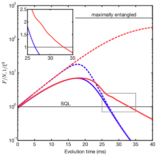
In the ideal case (constant parameters with and ) the early dynamics yield monotonically increasing Fisher information for an initial coherent spin state centered on the classically unstable fixed point (eigenstate of ). In contrast, the maximally attainable spin squeezing is limited due to the bending dynamics, which leads to an increase of the quantum uncertainty in all spin directions and a reduction of the spin squeezing for later evolution times. Fig. S2 shows numerical simulations of this ideal situation with typical experimental parameters of , and , where both Fisher information and spin squeezing have been optimized over rotation and measurement axis for each evolution time. This shows that the evolution creates non-Gaussian states useful for quantum metrology going beyond the quantum resources of the spin squeezed states accessible with this system. The Fisher information is found to saturate the Quantum Fisher Information for all evolution times, which is the maximum over all positive operator valued measures (POVM). This shows that the atomic imbalance stays the best observable. The experimentally observed decrease of the Fisher information as a function of time is a consequence of detection noise, technical imperfections and losses (detailed below). This basic behaviour is captured by including our detection noise of atoms as a Gaussian convolution of the theoretical probability distributions (Fig. S2, solid lines). The experimentally extracted Fisher information provides a lower bound for the quantum resources as it also includes all technical limitations. Since the quantum resources of the non-Gaussian states increasingly manifest themselves in substructures on small scales, they are especially affected by imperfect detection, which cannot resolve these features.
In the experimental system and are both a function of the atom number MicheliPRA2003 , caused by the dependence of the shape of the BEC mean-field order parameter and the mean atom density on . We find experimentally in good approximation with Hz and . The nonlinearity is for our range of atom numbers and for an initial atom number of . Besides noise effects, atom loss during the time evolution thus leads to a time dependence of these parameters.
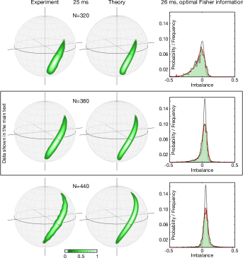
Due to these relations, the shape of the final state strongly depends on atom number, as depicted in Fig. S3. The Husimi distributions for the final atom numbers , and , obtained from the experimental tomographic reconstruction after an evolution time of , reveal a pronounced change in shape of the state with . This is consistent with a numerical simulation (Fig. S3 middle panel) taking into account the nonlinearity and detuning of . This includes the atom number dependence of the parameters during the time evolution, assuming with the experimentally determined decay time due to atom loss. All fast pulses (with in the Hamiltonian), including the spin-echo pulse in the middle of the time evolution, are modeled in the presence of nonlinearity and with a phase offset of °, which was employed in the experiment to compensate for nonlinearity during the initial preparation pulse. The experimentally observed shape is well explained by the assumed model. It is mainly the finite detuning which leads to the asymmetry of the final state. This is reflected in the Husimi projections and also shows up as an asymmetry of the experimental probability distributions for the tomography angle ° yielding maximal Fisher information (right column of Fig. S3 for an evolution time of ). For a comparison with the model, detection noise of the absorption imaging is taken into account by a convolution of the final distributions with a Gaussian of width atoms for (grey curves). Furthermore, the effect of particle loss of up to this evolution time leads to additional fluctuations which we estimate as , yielding a total width of atoms. With this convolution, the numerical simulations (red curves) are consistent with the observed experimental probability distributions.
Classical phase space
A useful insight to the dynamics is offered by the mean field picture which is exactly valid for and obtained by replacing the quantum mechanical operators by their mean values , where the imbalance is the normalized population difference and is the relative phase between the two internal states. In this limit, the dynamical evolution can be gathered in classical equations of motion of and its conjugate variable SmerziPRL ; ZiboldPRL2010 . The Hamiltonian becomes
| (S2) |
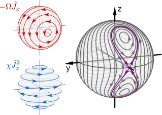
which is formally equivalent to a non-rigid pendulum, where . The equipotential lines of this classical Hamiltonian are the classical trajectories. These are shown in Fig. S1 for the three cases (red trajectories), (blue trajectories) and (gray trajectories), corresponding to the three cases of dominating Rabi coupling, dominating nonlinear evolution and the Josephson regime of weak Rabi coupling, respectively. For the topology of the phase space only depends on the parameter . For and the phase space features three stable fixed points and the unstable fixed point on the negative x-axis. An eight-shaped separatrix passing through the unstable fixed point divides the phase space into three regions of macroscopically different temporal behavior ZiboldPRL2010 ; SmerziPRL .
Experimental sequence
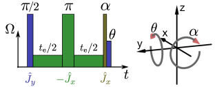
The experiment starts with a BEC of in each potential well. After ramping up the magnetic field to , a radio frequency rapid adiabatic passage transfers it to . In Fig. S4 we show schematically the experimental sequence beginning from this initial state. A fast Rabi pulse and subsequent non-adiabatic change of the driving phase by prepares each condensate in the coherent spin state , which corresponds to an independent superposition of each atom between the states and with the mean spin direction pointing towards the unstable fixed point. The state preparation pulses are sufficiently fast such that nonlinear effects induced by particle-particle interaction are negligible. The regime is addressed by attenuating the Rabi coupling strength below the nonlinear interaction . In the middle of the time evolution, a fast spin-echo pulse around the negative -axis is applied in order to further reduce the effect of shot-to-shot fluctuations of the detuning (caused by the finite magnetic field stability).
The Rabi pulses are implemented with microwave and radio frequency magnetic fields red-detuned with respect to the and transition, respectively. The resulting two-photon Rabi frequency for preparation, -pulse and tomography rotation is (corresponding to ) and is calibrated by Rabi flopping. The last -rotation is performed with an independently calibrated Rabi frequency of to reduce the influence of spurious timing and switching effects.
Spatial homogeneity
Special care has to be taken to ensure homogeneity of all applied fields along the one-dimensional lattice since we want lattice sites separated by up to to bear consistent conditions. We compensate the gradient of the magnetic offset field by adjusting small permanent magnets near the experimental chamber such that a magnetically sensitive microwave Ramsey sequence on the transition no longer shows any observable periodic pattern along the lattice. We note, that this measurement can be performed with higher accuracy than the on-site magnetic field stability because we have the advantage of the many-well information in every shot. It is only limited by the collisional (mean-field) shift of the two employed levels, which depends on the number of atoms on each lattice site. The relevant gradient of the microwave magnetic field can be measured by Rabi flopping on the transition with many cycles (), which eventually dephases along the lattice. This was minimized by small displacements of the microwave antenna and we find a remaining power gradient of over the whole ensemble which probably stems from the surrounding metal parts. For the fast rotation pulses, the influence of this remaining gradient on the homogeneity of the Rabi coupling is partly compensated by the gradient of the radio frequency power, which is on the same order but with opposite sign due to the special geometry and position of the coil of the radio frequency antenna. The remaining gradient of the Rabi coupling is over the whole BEC array, by which we can constrain the inhomogeneity of a -pulse to degrees in the relevant range of atom numbers with a maximum spacing of wells. This corresponds to of the width (2 standard deviations) of a coherent spin state with atoms.
For the two-photon coupling, the gradients of the off-resonant microwave and radio frequency driving also cause inhomogeneity of the AC Zeeman shifts. The absolute values are (microwave) and (radio frequency) which add up to total shift of the two-photon resonance in the case of the maximal power used for the fastest pulses. In order to reduce the influence of these gradients on the detuning during the time evolution, we distribute the attenuation over the two contributions. The microwave power is reduced by with an attenuator on a fast MW switch with two ports. The remaining attenuation needed to reach is achieved by reducing the power of the radio frequency. In this way, the gradient of the detuning during the time evolution can be reduced to below over the whole ensemble.
Long term stability and systematics
The most critical parameter in the experimental sequence is the detuning during the time evolution. Because the nonlinear term is on the order of , we have to work with Rabi frequencies of to obtain , which makes the system sensitive to detuning on the level of less than . Slow magnetic field changes due to small temperature drifts of the magnetic field sensor translate into detuning of . To obtain consistent conditions, we perform automated Ramsey experiments on the two-photon transition after 30-40 experimental repetitions and adjust the setpoint of the magnetic field stabilization accordingly. Compared to magnetic field measurements on a linear Zeeman sensitive transition, this has the advantage that small drifts of the AC Zeeman shift are also compensated. The additional information from these periodic reference measurements is used to filter out repetitions where subsequent Ramsey experiments differ by more than . Measurements of the Rabi frequency are performed on a daily basis and small drifts are corrected by slight adjustments of the radio frequency power.
Because of the dependence of the AC Zeeman shift on the power of the driving fields, special care was taken to ensure the resonance condition separately for all rotation pulses on the level of of the respective Rabi frequency. For this, we measure small amplitude Josephson oscillations with mean relative phase of (plasma oscillations) and ( oscillations) and adjust the detuning such that they both have the same amplitude and offset in the imbalance . The frequency difference of the same measurements is used to estimate the initial nonlinearity ZiboldPRL2010 .
Systematic overestimation of the Fisher information from the fits to the Hellinger distance could be caused by an underestimation of the effective Rabi frequency during the -rotation pulses. To minimize effects of switching, we attenuate the radio frequency and work with an offset rotation angle of 6 degrees. Thus the smallest angle (3.5 degrees, corresponding to degrees) still translates into a pulse duration of , which corresponds to cycles of the radio frequency. The rounding of the pulse length to full µs is included in the data analysis. From routinely performed measurements of the Rabi frequency, we can constrain the systematic error to which translates into an uncertainty of degrees and is negligible compared to the error bars of the squared Hellinger distance.
Experimental probability distributions
To obtain the experimental probability distributions for the Hellinger distance analysis, we collect the measurements of in bins of width after postselection for the total atom number . This width is slightly smaller than the experimental resolution due to photon shot-noise of atoms in the two population numbers and , which translates into an uncertainty of . By varying the bin width, we observe the expected saturation of the Hellinger distances for bin widths between and . The value is chosen to minimize artificial broadening of essential features of the distributions while still providing sufficient statistics in each bin. To obtain the experimental probabilities, each count is divided by the total number of counts in the distribution. For the Hellinger distance measurements, we typically collect experimental realizations at and at .
Reconstruction of the density matrix
For quantum state reconstruction, we collect the measurements of for each tomography angle in bins of width according to the granularity of the symmetric Hilbert space of with discrete eigenvalues of . We then use the iterative algorithm described in Lvovsky2004 to obtain a maximum likelihood estimate of the density matrix . For visualization, the Husimi projection on the coherent spin states ArecchiPRA1972
| (S3) |
with is calculated on a grid of points for the azimuthal angle and the polar angle , respectively. For the density plots in Fig. 2A of the main text, the obtained values are divided by their maximum.
Squeezing analysis
The separable coherent spin state (Eq. S3) has the binomial variance in , where . This is a consequence of the spin uncertainty of atoms independently prepared in the same superposition state. We refer to the value as number squeezing factor and to the value
| (S4) |
as spin squeezing factor. is the visibility of a perfect Ramsey experiment, which is limited by the elongation of the quantum state leading to a reduction of the mean spin length WinelandPRA1994 . We estimate from auxiliary interleaved measurements with the tomography angle that results in the biggest variance of (longest axis of the state). From these measurements, we deduce the normalized mean spin length . For the results shown in Fig. 2C of the main text, we average the values for at every tomography angle over all settings of . We note that reported results have not been corrected for detection or technical noise contributions. Values stated in dB are calculated as .
Fisher Information and Cramér-Rao bound
Let be the conditional probability distribution of the random variable , which continuously depends on the parameter , and an unbiased estimator of , i.e. , where indicates the expectation value. We start from the equalities
| (S5) | |||
| (S6) |
With the assumption that the summing range does not depend on , we get
| (S7) |
Taking the square of both sides, the Cauchy-Schwarz inequality , where and , yields
| (S8) |
We thus obtain the Cramér-Rao bound , where is the variance of the estimator and
| (S9) |
is the Fisher information. The extension to the case of independent measurements leads to HelstromBOOK , which is a natural extension obeying the extra scaling with for multiple measurements.
Extraction of the Fisher information from the Hellinger distance
We first illustrate the basic theory by considering the ideal situation where
the probabilities are known. Later we will consider the experimentally relevant case
where relative frequencies (experimental probabilities) are acquired.
Ideal case: probabilities.
The squared Hellinger distance between the probability distributions at and
at finite is
| (S10) |
where the sum, generally referred to as the Bhattacharyya coefficient (statistical fidelity or overlap), extends to all values of . For small , i.e. closely spaced probability distributions, the Taylor expansion of the squared Hellinger distance yields
| (S11) |
where
is the value of the Fisher information (Eq. S9)
at and its derivative.
The zeroth order of the Taylor expansion vanishes
because and the first order vanishes because
.
Thus, the Fisher information can be extracted from a polynomial
fit to by extracting the coefficient of the quadratic term.
Note, that , while and
the higher order terms of the expansion can also be negative.
By shifting the reference frame to , this procedure can easily be generalized
to obtain the Fisher information at arbitrary values of .
Experimental case: frequencies.
The method illustrated above to extract the Fisher information is valid for any state,
phase shift operation and measurement.
However, it requires the knowledge of the exact probability distributions.
The corresponding experimentally obtainable value is the
relative frequency (experimental probability) distribution for given ,
which approaches for infinitely many independent measurements.
We thus consider here the extraction of the Fisher information from a natural extension of the
Hellinger distance (Eq. S10),
| (S12) |
where and are the outcome frequencies obtained from a sample of experimental realizations. Due to statistical fluctuations, varies when repeating the measurement. We write
| (S13) |
where is the true underlying probability distribution (from which is sampled) and are the multinomial sampling errors characterized by
| (S14) | |||||
Because of the normalization, frequency fluctuations sum to zero: . We now expand Eq. S12 in the Taylor series around and . Since , this is justified if which, according to Eq. S14, corresponds to the condition . This is satisfied for sufficiently large. Taking the sample average, we find
| (S15) |
with
| (S16) | |||||
where is the number of discrete values of z for which . Since is the expectation value of at , we can estimate . We emphasize that the first order term in the -expansion of Eq. S12 vanishes. Notably, this happens also in the presence of frequency fluctuations. The estimation of the Hellinger distance with experimental probability distributions is asymptotically unbiased. The bias decreases with and is due to the finite fluctuations on the estimated probabilities and their strict positiveness. It can be reduced by employing a resampling procedure (see below). Regarding the statistical error of the Hellinger distance, we find
| (S17) |
Resampling procedure
Both and in Eq. S15 scale as , which is a prerequisite of the Jackknife procedure for bias reduction MillerBIOMETRICA1974 . We divide the experimental realizations in blocks of samples (). For the calculation of the Jackknife estimates we use , that is the squared Hellinger distance evaluated with the th group of experimental results of block size removed . The Jackknife estimator
| (S18) |
has the property to eliminate the -term from the estimate . Furthermore, the variance of is used to estimate the statistical uncertainty of . The results of this block-Jackknife are averaged up to blocksize for mean and variance. We verified the validity of this approach with Monte-Carlo simulations including realistic probability distributions and typical experimental sample sizes.
Bayesian estimation
Let be the true value of the phase shift and a sequence of independent measurement results, obtained with probability . The Bayes theorem
| (S19) |
assigns a probability distribution to the variable , conditioned by the measurement sequence . Here represents the prior knowledge about the phase shift which is assumed to be phase-independent in our analysis, and provides the normalization of . The shape of depends on the specific probabilities and on the observed results. Nevertheless, in the limit , becomes normally distributed, centered around the true value of the phase shift and with variance . This result is generally referred to as the Laplace-Bernstein-von Mises theorem LeCamBOOK . To demonstrate it, we rewrite in terms of frequencies to observe the result : , where the proportionality sign indicates equality up to a normalization constant. In the limit , frequencies tend to probabilities () and thus
| (S20) |
where the constant term contains the normalization of . We now expand this equation in the Taylor series around the maximum of . First, the condition is satisfied if . We will assume that is the only maximum of Eq. S20. Up to the leading order in and neglecting constant terms, which are absorbed in the normalization of , we thus have
| (S21) |
The fact that guarantees that higher order terms of the expansion are negligible for .
For the Bayesian analysis presented in the main text we take advantage of the fact that the experimental probability distribution used as (reference) for the calculation of the Hellinger distance was collected with approximately four times the experimental repetitions compared to . We randomly draw 1000 repetitions of this setting and use the remaining ones to generate the distribution . We then determine the region , where for all . The 1000 repetitions are used as independent realizations for Bayesian estimation of and grouped in -sequences . For each -sequence we calculate the likelihood (equivalent to without normalization and ) for the (discrete) values of for which experimental probabilities are available. Realizations with for some , i.e. outside the range are discarded. This is an essential step to obtain a finite value of the likelihood for each sequence. Note, that we do not reduce the value of in this step. Discarding too many realizations would thus show up as reduced sensitivity in the further analysis.
We use no prior knowledge on the phase shift, i.e. . As discussed above, we expect and thus the likelihood to be normally distributed around the true value of the phase shift . We thus fit the results for quadratically and extract from the curvature of the fit. As discussed in the main text, for sufficiently large (see Fig. 4), we get , where agrees with the value of the Fisher information obtained with the Hellinger distance method.