Complex network based techniques to identify extreme events and (sudden) transitions in spatio-temporal systems

Abstract

We present here two promising techniques for the application of the complex network approach to continuous spatio-temporal systems that have been developed in the last decade and show large potential for future application and development of complex systems analysis. First, we discuss the transforming of a time series from such systems to a complex network. The natural approach is to calculate the recurrence matrix and interpret such as the adjacency matrix of an associated complex network, called recurrence network. Using complex network measures, such as transitivity coefficient, we demonstrate that this approach is very efficient for identifying qualitative transitions in observational data, e.g., when analyzing paleoclimate regime transitions. Second, we demonstrate the use of directed spatial networks constructed from spatio-temporal measurements of such systems that can be derived from the synchronized-in-time occurrence of extreme events in different spatial regions. Although there are many possibilities to investigate such spatial networks, we present here the new measure of network divergence and how it can be used to develop a prediction scheme of extreme rainfall events.

In the last decades various powerful techniques have been developed in nonlinear dynamics for the study of continuous spatio-temporal dynamic systems. Typically they are based on different discretization methods in space and time. Here, we discuss an unconventional approach based on complex networks for the investigation of such systems. In contrast to well-known examples of complex networks, such as social ensembles, neural networks, or power grids, where the nodes are clearly defined by humans, neurons or power generating stations, here the first step of the complex network approach can be interpreted as a very flexible way to discretize a continuous system, or to identify a backbone underlying the continuous system. This enables us to use in the next steps the rich variety of methods from complex network theory even for the analysis of continuous systems. Based on this approach we treat two basic problems in high-dimensional nonlinear dynamics: (i) uncovering regime shifts and (ii) prediction of extreme events. We propose appropriate techniques for both by combining recurrence with networks resp. synchronization with extreme events. The potential of this approach is demonstrated here for the Earth system. In a first example we show that important main regime shifts of the East Asian Monsoon during the last 3 Million years can be identified from paleoclimate proxy records. In a second example we analyze recent satellite data from the tropical rainfall measurement mission (TRMM) and use the network divergence for developing an efficient prediction scheme for extreme precipitation events in the eastern Central Andes.

I Introduction

Climate is as the brain a highly complex and high-dimensional system; both systems have a lot of joint properties, but there are also important distinctions. Understanding the mechanisms of climatic processes on all temporal and spatial scales is very difficult and even impossible in near future, but crucial for weather forecasts or assessment of long-term climate changes. A data-based investigation of the climate system is related with several challenges, in particular non-stationarity (e.g., abrupt vs. slow changes), high-dimensionality, non-Gaussian distributed data (e.g., extreme events), natural vs. anthropogenic influences, etc.

A basic first step in data-based studies of such a complex high-dimensional system is reducing the dimensionality. The most widely used method for this is a decomposition into a very finite number of Empirical Orthogonal Functions (EOFs). This approach also allows to identify main spatial patterns, such as large circulation patterns or teleconnections. However, the basis of the EOF approach is the covariance matrix, thus, only capturing the first two statistical moments and demanding for certain strict properties of the data, e.g., Gaussian distribution and stationarity Monahan et al. (2009). Even more obvious are constraints due to event-like data, as typical for rainfall and extreme events, or limitations by nonlinear interrelations. Moreover, the found EOFs do not undoubtedly coincide with typical climate phenomena Dommenget and Latif (2002).

Modern measurement techniques has allowed in the last decades to extend our knowledge into the past, leading to paleoclimatology. However, these data generate further challenges: Dating uncertainties and irregularly sampled time series are problems that limit the direct application of standard methods.

An alternative and novel approach for the study of different aspects of the climate system is related to the progress in complex networks science in the past quarter century. At a first glance it might appear surprising that the complex network approach can be used to analyse a continuous system as the climate and in particular to identify spatio-temporal patterns in climate fields or regime shifts in the paleoclimate. However, the application of complex networks for climate analysis has become a lively and quickly progressive field in the last years. Although, this new approach is still in its infancy, first results are very promising and have already shown its impressive potential.

In the following we will present two techniques based on complex networks, recurrence networks (Sec. III) and event synchronization (Sec. V), and will show how they can be used to uncover regime transitions in the paleoclimate by analyzing proxy records (Sec. IV) and to analyze spatiotemporal patterns of extreme rainfall leading to new prediction schemes (Sec. V). Finally we summarize the potentials of this non-traditional approach, but discuss also open problems.

II Complex networks

We give here only a few basics on complex networks which will be used later (see, e.g., Strogatz (2001); Newman (2003); Boccaletti et al. (2006) for more detailed reviews on complex network analysis). A network is a set of nodes and links. We define a network as complex when its topology is highly irregular. A network can be defined by the adjacency matrix $\mathbf{A}$. For undirected and unweighted networks, $\mathbf{A}$ is a binary matrix, just indicating the existence of links between two nodes. In weighted networks, a link has a weight, i.e., $\mathbf{A}$ consists of real numbers; $\mathbf{A}$ is symmetric for undirected and asymmetric for directed networks. A network or its components (links, nodes) can be characterized by several measures. Here we mention only some selected measures.

The node degree in unweighted networks is simply the total number of links a node $i$ has and is given by the column sum of the adjacency matrix $\mathbf{A}$:

$$k_{i}=\sum_{j}^{N}A_{ji}.$$ (1)

The distribution of this measure can be used to investigate, e.g., whether a network is scale-free. On directed networks, we can distinguish between the column-wise and raw-wise sums in Eq. (1) that give us the in- and out-degree, respectively. For weighted networks the sum Eq. (1) becomes the so-called node strength, and for directed and weighted networks, we can consider the in- and out-strength

$$\mathcal{S}_{i}^{\text{in}}=\sum_{j=1}^{N}A_{ij}\quad\text{and}\quad\mathcal{S}_{i}^{\text{out}}=\sum_{j=1}^{N}A_{ji}.$$ (2)

Another important measure is the transitivity coefficient

$$\mathcal{T}=\frac{\sum_{i,j,k=1}^{N}A_{j,k}A_{i,j}A_{i,k}}{\sum_{i,j,k=1}^{N}A_{i,j}A_{i,k}}.$$ (3)

It measures the probability that the neighbors of a node are connected themselves.

III Recurrence Networks – a time series analysis approach by means of complex networks

Analyzing time series by complex networks is a quite new idea that came up in the last decade. The generation of a complex network representation of a time series can be done using different approaches, e.g., by visibility graphs Lacasa et al. (2008) or temporal succession of local rank orders Small (2013). A quite natural approach is to use the recurrence matrix Marwan et al. (2007) of a dynamical system

$$R_{i,j}=\Theta(\varepsilon-||\vec{x}(i)-\vec{x}(j)||),$$ (4)

as the adjacency matrix of a complex network Donner et al. (2011a):

$$\mathbf{A}=\mathbf{R}-\mathbb{I}$$ (5)

(with $\mathbb{I}$ the identity matrix, $\Theta$ the Heaviside function, $\vec{x}(i)$ a state at time $i=1,\ldots,N$, and $N$ the number of state vectors). The recurrence matrix itself has become a basic tool of nonlinear time series analysis and was first introduced by Eckmann et al. as recurrence plots that “are rather easily obtained aids for the diagnosis of dynamical systems” Eckmann et al. (1987). Later this idea was extended by several quantification approaches Zbilut and Webber, Jr. (1992); Marwan et al. (2002) leading to “an active field, with many ramifications we [Eckmann et al. – ] had not anticipated” Marwan et al. (2008). Fundamental works on such methodological developments have been published also in Chaos, e.g., on embedding issues and dynamical invariants Iwanski and Bradley (1998); Thiel et al. (2004), time-delay systems and non-chaotic strange attractors Senthilkumar et al. (2008); Ngamga et al. (2008), heterogenous recurrence analysis Yang and Chen (2014), or twin surrogates Romano et al. (2009).

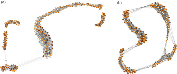
Because of the striking similarity between the recurrence matrix and the adjacency matrix (i.e., a binary and square matrix), the idea to identify the recurrence matrix with the adjacency matrix was so obvious that it came up almost at the same time (around 2008) within different research groups Xu et al. (2008); Marwan et al. (2009); Strozzi et al. (2009). Its main advantage is that the resulting recurrence network can be analyzed by the known network measures, i.e., further diagnostic tools become available for time series analysis. In particular the transitivity coefficient $\mathcal{T}$ is appropriate because it quantifies the geometry of the phase space trajectory and can be used to differentiate between different dynamics (e.g., regular and irregular) Marwan et al. (2009); Zou et al. (2010). It also allows to define a dimensionality measure Donner et al. (2011b), the transitivity dimension

$$D_{\mathcal{T}}=\frac{\log(\mathcal{T})}{log(3/4)}.$$ (6)

The quantification of the recurrence matrices can also be performed by the recurrence quantification analysis (RQA) Marwan et al. (2007); Webber, Jr. and Marwan (2015). In contrast to the network measures which describe the geometrical properties, the RQA measures characterize dynamical properties of the phase space trajectory. Therefore, the recurrence network based measures provide complementary information to the RQA and can, under certain circumstances, give more insights into the system’s behavior.

As a paradigmatic example, let us consider the Rössler system Rössler (1976)

$$\left(\frac{dx}{dt},\,\frac{dy}{dt},\,\frac{dz}{dt}\right)=\bigl{(}-y-z,\ x+ay,\ b+z(x-35)\bigr{)},$$ (7)

where we change the parameter $a=b$ in a range where the system shows chaotic and periodic dynamics: $a=0.235,\ldots,0.262$ (Figs. 1 and 2). Between $a=0.24$ and 0.25, the system does not have a positive Lyapunov exponent and generates periodic behavior (Fig. 3(a)).

Figure 1: (a) Phase space reconstruction of the $x$-component of the Rössler system for $a=0.245$ and (b) for $a=0.29$. (c) Corresponding recurrence plot for $a=0.245$, showing periodic structures, and (d) for $a=0.29$, showing interrupted diagonal lines. The recurrence plots are calculated from the $x$-component using time-delay embedding with $m=4$ and $\tau=17$ (sampling time $\Delta t=0.1$).

Figure 2: Network representation of the phase space reconstruction of the $x$-component of the Rössler system for (a) $a=0.245$ and (b) $a=0.29$. The network is constructed from the first 300 nodes of the recurrence matrix shown in Fig. 1 by a linear repulsion model. Node size and color can be used to represent selected node properties, here time (node color, the darker the larger $t$) and clustering coefficient (node size).

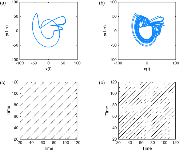
A frequently used RQA measure for differentiating periodic and chaotic dynamics is the ratio of recurrence points that form diagonal lines in the recurrence plot, called determinism Trulla et al. (1996); Marwan et al. (2007):

$$DET=\frac{\sum_{l\geq l_{\min}}lP(l)}{\sum_{i,j}R_{i,j}},$$ (8)

with $P(l)$ the histogram of line lengths in the recurrence plot. The idea of this measure is that the length of a diagonal line in the recurrence plot corresponds to the time the system evolves very similar as during another time. Such repeated similar state evolution that is also related to predictability is typical for deterministic systems. In contrast, systems with independent subsequent values, like white noise, have mostly single points in the recurrence plot. DET is sensitive to transitions between chaotic and periodic dynamics in maps Trulla et al. (1996), but for continuous systems, such as our Rössler example, this measure fails for this task Zou et al. (2010); Marwan (2011). For the entire range of the considered $a$ values, it has very high values, close to one (Fig. 3(b), Tab. 1). However, $\mathcal{T}$ shows increased values within the periodic window, close to a value of $3/4$. In general, the network based measures, such as $\mathcal{T}$, can add further important aspects in recurrence analysis, in particular for the uncovering of sudden changes of the dynamics.

Figure 3: (a) The two largest Lyapunov exponents and (b) the recurrence measures DET and $\mathcal{T}$ for the $x$-component of the Rössler system for varying control parameter $a$. Within the interval $a=[0.24\ 0.25]$, the dynamics is periodic. Whereas $\mathcal{T}$ indicates the periodic behavior by increased values, it is difficult to detect the periodic window with DET Marwan (2011).

Table 1: Typical values of DET and $\mathcal{T}$ for different dynamical regimes in the Rössler system.

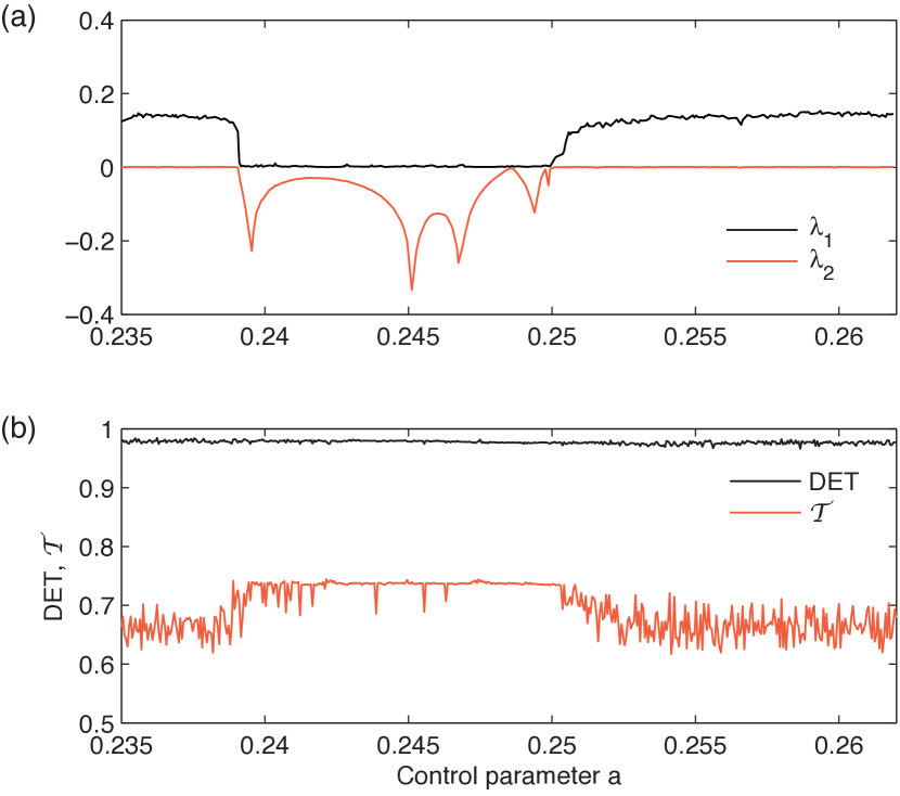
$a$	DET	$\mathcal{T}$	dynamics
0.235	0.98	0.66	chaotic
0.245	0.98	0.74	periodic
0.260	0.97	0.63	chaotic

IV Identification of sudden transitions in paleoclimate

The recurrence network approach has great potential in different applications in many disciplines. Using as a classifier, it can help, e.g., to detect serious diseases, such as preeclampsia Ramírez Ávila et al. (2013), to detect epileptic states Lang et al. (2013), or to study multiphase fluid flows Gao et al. (2013). Another important application is to detect critical transitions in the dynamics Marwan et al. (2009); Donges et al. (2011a); Eroglu et al. (2014). Such transition detection is of crucial interest in studying variations of the past climate in order to better understand the climate system in general.

In the following we discuss a typical example from paleoclimate research. The investigation of relationships between sea surface temperature (SST) and specific climate responses, like the Asian monsoon system or the thermohaline circulation in the Atlantic, as well as their regime changes, represents an important scientific challenge for understanding the global climate system, its mechanisms, and its related variability. Its better understanding is of crucial importance as non-linear feedback mechanisms and tipping points cause high uncertainty and an unpredictable future for humankindLenton et al. (2008); Rockstrom et al. (2009).

In paleoclimatology, different archives are used to reconstruct and study climate conditions of the past, as lake Marwan et al. (2003) and marine sediments Herbert et al. (2010) or speleothemes Kennett et al. (2012). Alkenone remnants in the organic fraction of marine sediments, produced by phytoplankton, can be used to reconstruct SST of the past (alkenone paleothermometry), allowing to study the temperature variability of the oceans Herbert (2001); Li et al. (2011). Here we will use a SST reconstruction for the South China Sea and the past 3 Ma derived from alkenone paleothermometry of the Ocean Drilling Programme (ODP) site 1143Li et al. (2011) (Fig. 4 and 5(a)). The South China Sea is strongly linked to the East Asian Monsoon system (EAM) that consists of a winter part with strong winds and a precipitation related summer part. In general, the East Asian Monsoon is of crucial importance for China’s socio-economic behavior, e.g., for agriculture or even for public health by its impact on prevalence of trace elements Blazina et al. (2014). The understanding of the mechanism is, therefore, crucial for learning about the past and the future climate and its impacts.

Figure 4: Location of the ODP 1143 site in the South China Sea (red star) and main directions of the East Asian Summer Monsoon (blue arrows).

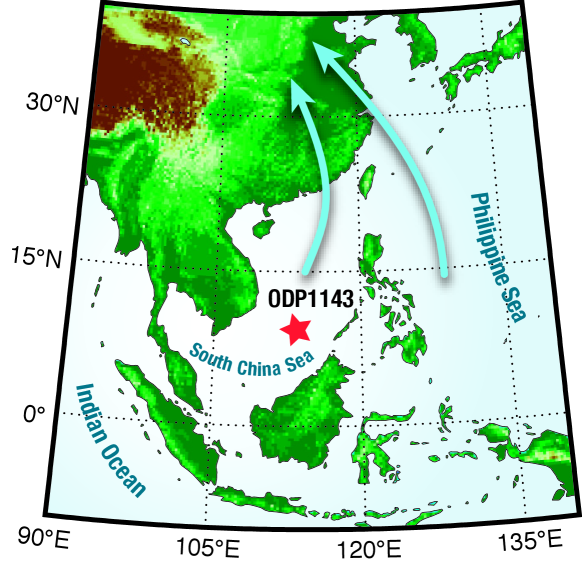
First we are faced with a typical problem in paleoclimatology because the original time series of ODP 1143 is not equally sampled. The sampling time ranges from 0.2 to 28 ka, with a median of 2.1 ka. If applying standard techniques (linear methods or classical RQA) then we would first need to interpolate the time series to an equidistant time axis. However, when using the recurrence network approach, the correct timing of the nodes is not so important (and could even be exchanged without changing the network properties), because it is characterizing the geometrical structure Donges et al. (2011b, a); Feldhoff et al. (2012).

We calculate the recurrence networks and the transitivity coefficient $\mathcal{T}$ for sliding windows of length 410 ka (thus, with varying number of data points within the windows) and a moving step of 20 ka (Fig. 5). For the phase space reconstructionPackard et al. (1980) we choose an embedding dimension of $m=6$ (as suggested by the false nearest neighbors methodKennel et al. (1992)). The selection of the time delay is guided by the auto-correlation function and considered to be constant for all time windows to be approximately 20 ka (based on median sampling time within one time window). The threshold is chosen in such a way to preserve a constant recurrence rate of 7.5% Marwan et al. (2007); Donges et al. (2011a).

Moreover, we perform a bootstrapping approach using 1,000 resamplings of the windowed time series for preparing an empirical test distribution for $\mathcal{T}$. In this real world example, we use a confidence level of 90%. As we do not know which kinds of dynamical transition are there, we will consider both the upper and the lower confidence level.

Figure 5: (a) Alkenone paleothermometry based SST estimates for the South China Sea and (b) corresponding transitivity coefficient $\mathcal{T}$. Dashed lines mark major climate shifts discussed in the text; the gray shading marks the confidence interval of 90%.

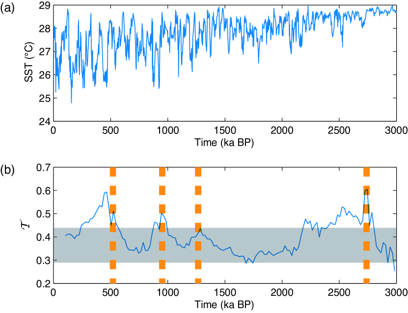
In the last 3 Ma several major and many smaller climate changes have appeared on regional but also global scale. Dramatic climate shifts are related with the Milankovich cycles Haug and Tiedemann (1998); Medina-Elizalde and Lea (2005); An (2014) and major changes in ocean circulation patterns Karas et al. (2009). Due to a transition towards an obliquity-driven climate variability with a 41 ka period around 3.0 Ma ago, a period of warm climate has end and the northern hemisphere glaciation started after 2.8–2.7 Ma Haug and Tiedemann (1998); Herbert et al. (2010); An (2014). This transition is very well revealed by the significant increase of $\mathcal{T}$ between 2.8 and 2.2 Ma. Based on thorough investigations of loess sediments, it is known that 1.25 Ma ago the intensity of the winter monsoon of the EAM begun to be strongly coupled to global ice-volume change An (2014). During this time, $\mathcal{T}$ increased (although not reaching significance). This time also marks the beginning of a transition phase towards glacial-interglacial cycles of 100 ka period (eccentricity dominated period of the Milankovich cycles). This 100 ka period dominance was well established after 0.6 ka and is clearly visible by the increased $\mathcal{T}$ between 0.6 and 0.2 ka Sun et al. (2010). From loess sediments it is also known that the summer monsoon has weakened between 2.0 and 1.5 ka and around 0.7 ka. During these periods, $\mathcal{T}$ shows lower values than during the previously discussed periods. The variation of $\mathcal{T}$ confirms the previous findings of a strong link between the EAM and the Milankovich cycles, in particular of increased and reduced regularity in the climate dynamics (as presented by the SST and for the considered time scale) during dominant Milankovich cycles and periods of major climate transitions from one to another regime.

Similar conclusions based on $\mathcal{T}$ have been drawn from dust flux records around the African continent Donges et al. (2011a). There, it was found that enhanced regular climate dynamics coincides well with lake level high stands in East Africa and, hence, indicating that climate regime transitions have triggered human evolution.

V Complex networks for spatio-temporal analysis of continuous systems

Another important problem in complex systems analysis is the investigation of spatio-temporal dynamics. In the last decade, this field has also benefited from the complex network approach. In particular, its application on climate data in order to uncover climate mechanisms or characteristic spatial patterns and long-range interrelations has drawn attention to complex networks for spatio-temporal analysis of continuous systems. Complex networks are an alternative to EOFs and can shed light on different and complimentary aspects than EOFs. Beginning with the study of Tsonis et al. in 2004 Tsonis and Roebber (2004), the climate network approach has received more and more interest for spatio-temporal data analysisEbert-Uphoff and Deng (2012); van der Mheen et al. (2013); Stolbova et al. (2014). The idea is to reconstruct a complex network from spatially embedded time series (in case of climate, e.g., from a surface air temperature field) by measuring the interrelationship $C_{i,j}$ between these time series. The location of the nodes can be arbitrary (e.g., weather stations when using instrumental data) or grid points (e.g., when using model or reanalysis data). In unweighted networks, links represent high correlations between the time series belonging to the nodes, simply considered by applying a threshold $T$ on the interrelation matrix $\mathbf{C}$ (that could be, e.g., Pearson correlation)

$$A_{i,j}=\left\{\begin{array}[]{l l}C_{i,j}&\quad\text{if}\quad C_{i,j}>T,\\ 0&\quad\text{else}.\\ \end{array}\right.$$ (9)

Such networks can be undirected or unweighted (as in Eq. (9)), but also directed or weighted.

Within the climate context, such network approach has been applied to study, e.g, climate communities Tsonis and Roebber (2004); Steinhaeuser and Chawla (2010), the impact of the El Niño/ Southern Oscillation Yamasaki et al. (2008), major heat transport pathways and spatio-temporal scales Donges et al. (2009a); Ebert-Uphoff and Deng (2012), external and internal atmospheric forcingDeza et al. (2014), to create early warning indicators of critical regime shifts van der Mheen et al. (2013), or even for model intercomparison Steinhaeuser and Tsonis (2013); Feldhoff et al. (2014). When using Pearson correlation for describing the interrelationships $C_{i,j}$ between the nodes, then the node degree is obviously related to the first EOF Donges et al. (2015). Other network measures, such as betweenness centrality, provide further information that cannot be captured by the EOF analysis Donges et al. (2009a).

In general, interrelationships between spatially located time series cannot be considered to be only linear. In order to examine nonlinear interrelations, information based measures (e.g., mutual information) were suggested for network reconstruction Donges et al. (2009b); Barreiro et al. (2011); Runge et al. (2012); Deza et al. (2013); Hlinka et al. (2013). In particular when investigating climatological or meteorological phenomena, we often face event-like data, such as daily (or hourly) rainfall series or extreme events time series. For such kind of data, Spearman rank correlation could be used Carpi et al. (2012). However, an even more powerful approach for such data is the event synchronization approach Quian Quiroga et al. (2002); Malik et al. (2010).

Event synchronization was developed to investigate the synchronous activity of the neurons in the brain Quian Quiroga et al. (2002). It simply counts the number of temporally coinciding events in two event series $x_{1}$ and $x_{2}$ by allowing small deviations between the occurrence of the events, i.e., a dynamical delay between them. Let $e_{1}(m)$ and $e_{2}(n)$ be the time indices when events appear in $x_{1}$ and $x_{2}$ and $m,n=1,\ldots,l$ the number of a specific event ($l$ is the total number of events in the event series). The waiting time between an event $m$ in $x_{1}$ and event $n$ in $x_{2}$ is $d_{1,2}(m,n)=e_{1}(m)-e_{2}(n)$. If this waiting time $d_{1,2}(m,n)$ is smaller than some dynamical delay $\tau(m,n)$, the two events $e_{1}(m)$ and $e_{2}(n)$ are considered to occur synchronously. The dynamical delay $\tau(m,n)$ is the half of the minimal waiting time of subsequent events in both time series around event $e_{1}(m)$ and $e_{2}(n)$ and not larger than a given maximal delay $\tau_{\max}$, i.e.,

$$\tau(m,n)=\min\frac{\{d_{11}(m,m-1),d_{11}(m,m+1),d_{22}(n,n-1),d_{22}(n,n+1),2\tau_{\max}\}}{2}.$$ (10)

As soon as $|d_{1,2}(m,n)|\leq\tau(m,n)$ (or $0<d_{1,2}(m,n)\leq\tau(m,n)$), we count it as undirected (or directed) synchronization of events $e_{1}(m)$ and $e_{2}(n)$

$$S(m,n)=\left\{\begin{array}[]{l l}1&\quad\text{if}\quad|d_{1,2}(m,n)|\leq\tau(m,n)\\ &\quad(\text{or}\ 0<d_{1,2}(m,n)\leq\tau(m,n)\ \text{in the directed case}),\\ 0&\quad\text{else}.\\ \end{array}\right.$$ (11)

Now we can define the event synchronization $E$ between the two event series as the sum of $S(m,n)$

$$E=\sum_{m,n}S(m,n).$$ (12)

This measure has the advantage that it can quantify interrelations between event-like time series and that it allows for a flexible (dynamical) delay between the events. This is particularly different from the standard approach, where a considered lag (e.g., for cross-correlation) is constant and fixed at each time point.

Applying the event synchronization approach, Eq. (12), for comparing spatially embedded time series $x_{i}$ and $x_{j}$ at locations (nodes) $i$ and $j$ a network can be reconstructed in the same way as in Eq. (9). For selecting the threshold $T$ several approaches are possible. One possibility is based on a significance test, where block bootstrapping can provide an empirical test distribution of the values of $\mathbf{E}$ and a preselected confidence level (e.g., 2% or 5%) provides the threshold $T$Boers et al. (2014). This procedure ensures that the network links represent only the strongest interrelations between the nodes.

Event synchronization based complex networks have been successfully used to investigate spatio-temporal patterns during the Indian Summer monsoon Malik et al. (2010, 2012); Stolbova et al. (2014) or to study the origin and propagation of extreme rainfall in South America Boers et al. (2013, 2014). Although there is an obvious dominance of climate applications, this approach is also promising for other fields, like plasma, turbulence, cardiological, or brain research.

VI Developing a prediction scheme for extreme events

To illustrate the potential of the complex network approach in the context of extreme climate events, we apply the approach on South American extreme rainfall data and use the network topology for developing a prediction scheme for extreme rainfall Boers et al. (2014). During the Australian summer season (December, January, February), the differential heating between land and ocean amplifies the trade winds that enhances transport of moisture from the tropical Atlantic into the tropical Amazonian Basin and, thus, causes extended rainfallZhou and Lau (1998). Due to evapotranspiration, wind, and the Andean orographic barrier, this water is first further transported westwards and later, along the Andean mountain ridge, southwards towards the subtropics (Fig. 6). Here, a frontal system converging from the South and related with Rossby waves is responsible whether the moisture transport moves further eastward into the southeastern (SE) Brazil or towards the SE South America (SESA, central Argentinian plains)Marengo et al. (2004). This variability of the exit moisture regions is also called South American rainfall dipole Nogués-Paegle and Mo (1997).

Figure 6: Key features of the South American monsoon system. The blue arrows indicate major moisture transport pathways.

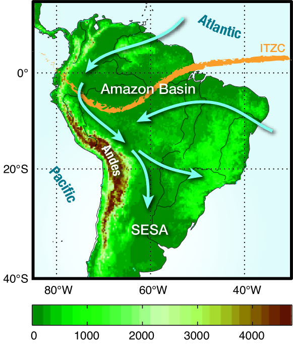
The spatio-temporal rainfall data used in our example is collected from the satellite-based Tropical Rainfall Measurement Mission (TRMM 3B42 V7, Huffman et al. (2007)) with $3$-hourly temporal and $0.25^{\circ}\times 0.25^{\circ}$ spatial resolution. In the following we will restrict the analysis to the Australian summer season and consider extreme rainfall events that are defined locally by rainfall exceeding the $99$th percentile.

Using directed event synchronization, Eqs. (11–12), of the rainfall extremes we reconstruct weighted and directed networks and calculate the in-strength $\mathcal{S}_{i}^{\text{in}}$ and out-strength $\mathcal{S}_{i}^{\text{out}}$, Eq. (2). Now we define the network divergence as the difference between in- and out-strength:

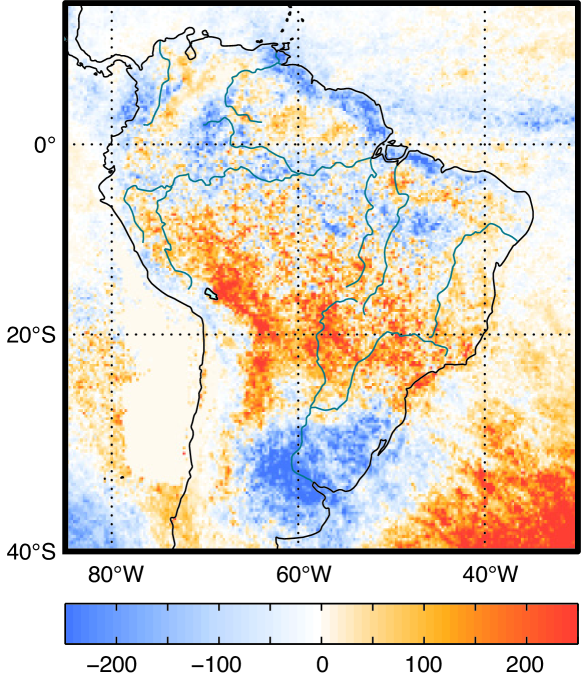
$$\Delta\mathcal{S}_{i}=\mathcal{S}_{i}^{\text{in}}-\mathcal{S}_{i}^{\text{out}}.$$ (13)

Negative values of $\Delta\mathcal{S}$ indicate the source regions of extreme events whereas positive values indicate sinks. Surprisingly, we find negative $\Delta\mathcal{S}$ values within the SESA region (Fig. 7). This means that this region is a source region of extreme rainfall although it is one of the exit regions of the low-level moisture flow from the Amazon region. Now it would be interesting to see to which other places the extreme rainfall from the SESA region will propagate. For this purpose we consider the in-strength of all nodes conditioned by the source region SESA and call it impact $\mathcal{I}_{i}(R)$ of region $R$ on node $i$:

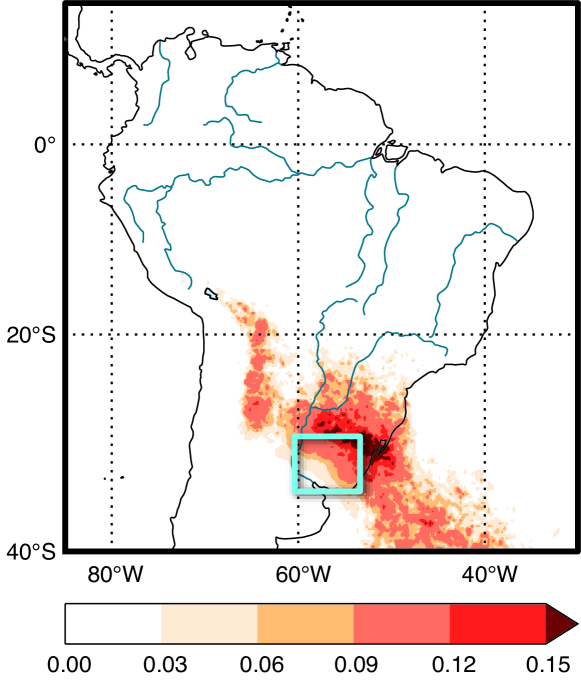
$$\mathcal{I}_{i}(R):=\frac{1}{|R|}\sum_{j\in R}A_{ij}.$$ (14)

$|R|$ is the number of nodes within the region of interest $R$ (here SESA). Casually speaking, $\mathcal{I}_{i}(R)$ measures the amount of extremes at site $i$ that have their origin in region $R$.

For the SESA region we find high values of $\mathcal{I}_{i}(\text{SESA})$ not only in the direct vicinity of SESA but also at the eastern slopes of the Central Andes (Fig. 8). This result suggests that extreme rainfall at the Central (in particular Bolivian) Andes will precede after rainfall events in the SESA region.

The mechanism behind this is an interplay between the orographic barrier, frontal systems approaching from the South, and the southward moisture flow from the Amazon basin resulting in the establishment of a wind channel attracting warm and moist air from the western Amazon region into the SESA regionBoers et al. (2014). Here it collides with the cold air of the frontal system from the South and produces extended rainfall. This rainfall propagates together with the northern migration of the frontal system and is bounded in the West by the Andean orography.

This fact can be used for defining a simple but very efficient prediction scheme as explained in detail by Boers et al.Boers et al. (2014) The precondition is a low-pressure anomaly in the SESA (geopotential height anomaly $<-10$ m). As long as this condition is fulfilled, during two days extreme rainfall will appear at the eastern slopes of the Central Andes (in the range along the band that is marked by high values of $\mathcal{I}_{i}(\text{SESA}))$. This rule allows positive prediction rates of 60% and during El Niño conditions even of 90%.

Figure 7: Network divergence $\Delta\mathcal{S}$ of extreme rainfall network during Austral winter season. Negative values indicate source and positive values sink regions of extreme rainfall.

Figure 8: Impact $\mathcal{I}_{i}(R)$ of a region (here SESA, marked by the box) in form of contributing propagated extreme rainfall.

VII Conclusion and Outlook

In this paper we have presented an overview of a complex network based method for the analysis of continuous dynamical systems. These methods are mainly basing on two concepts: (i) recurrence networks and (ii) event synchronization. The first one combines recurrence, a basic principle in dynamical systems, with complex networks. This way a rich variety of complex networks characteristics become available for time series analysis. Its potential have been demonstrated for the identification of sudden transitions from even short time series. The second one identifies events occurring almost synchronized in time in different spatial regions and uses then complex networks for the study of especially spreading and interactions of extreme events. We have uncovered with this technique a mechanism for the formation of extreme floods in the Andes which has led to a very efficient framework for predicting such extreme events. Additionally, this methodology can be used as a new tool for a critical comparison of different models of in particular natural systems. Such complex network approaches have a strong potential for various fields, ranging from turbulence, via neuroscience and medicine to socio-economy.

However, there are several open problems to study in future. One direction is to extend these concepts to multivariate (spatio-temporal) data, e.g., different climatological or physiological parameters. A further challenge is the study of interacting systems of possible very different nature, e.g., climate and renewable energy generation or climate and health, from the network perspective. Another problem is a comprehensive mathematical foundation of these techniques including an appropriate test statistics. Thus, we expect a pursuing and lively development and an increasing number of applications of these rather new concepts in the next future.

VIII Acknowledgement

We would like to acknowledge support from the IRTG 1740/TRP 2011/50151-0, funded by the DFG/FAPESP, the DFG project “Investigation of past and present climate dynamics and its stability by means of a spatio-temporal analysis of climate data using complex networks” (MA 4759/4-1), and project “Gradual environmental change versus single catastrophe – Identifying drivers of mammalian evolution” (SAW-2013-IZW-2), funded by the Leibniz Association (WGL). Moreover, we thank Niklas Boers for helpful comments.

References

- Monahan et al. (2009) A. H. Monahan, J. C. Fyfe, M. H. P. Ambaum, D. B. Stephenson, and G. R. North, Journal of Climate 22, 6501 (2009).
- Dommenget and Latif (2002) D. Dommenget and M. Latif, Journal of Climate 15, 216 (2002).
- Strogatz (2001) S. H. Strogatz, Nature 410, 268 (2001).
- Newman (2003) M. Newman, SIAM review 45, 167 (2003).
- Boccaletti et al. (2006) S. Boccaletti, V. Latora, Y. Moreno, M. Chavez, and D. U. Hwang, Physics Reports 424, 175 (2006).
- Lacasa et al. (2008) L. Lacasa, B. Luque, F. Ballesteros, J. Luque, and J. C. Nuño, Proceedings of the National Academy of Sciences 105, 4972 (2008).
- Small (2013) M. Small, in IEEE International Symposium on Circuits and Systems (ISCAS2013) (2013) pp. 2509–2512.
- Marwan et al. (2007) N. Marwan, M. C. Romano, M. Thiel, and J. Kurths, Physics Reports 438, 237 (2007).
- Donner et al. (2011a) R. V. Donner, M. Small, J. F. Donges, N. Marwan, Y. Zou, R. Xiang, and J. Kurths, International Journal of Bifurcation and Chaos 21, 1019 (2011a).
- Eckmann et al. (1987) J.-P. Eckmann, S. Oliffson Kamphorst, and D. Ruelle, Europhysics Letters 4, 973 (1987).
- Zbilut and Webber, Jr. (1992) J. P. Zbilut and C. L. Webber, Jr., Physics Letters A 171, 199 (1992).
- Marwan et al. (2002) N. Marwan, N. Wessel, U. Meyerfeldt, A. Schirdewan, and J. Kurths, Physical Review E 66, 026702 (2002).
- Marwan et al. (2008) N. Marwan, A. Facchini, M. Thiel, J. P. Zbilut, and H. Kantz, European Physical Journal – Special Topics 164, 1 (2008).
- Iwanski and Bradley (1998) J. S. Iwanski and E. Bradley, Chaos 8, 861 (1998).
- Thiel et al. (2004) M. Thiel, M. C. Romano, P. L. Read, and J. Kurths, Chaos 14, 234 (2004).
- Senthilkumar et al. (2008) D. V. Senthilkumar, M. Lakshmanan, and J. Kurths, Chaos 18, 023118 (2008).
- Ngamga et al. (2008) E. J. Ngamga, A. Buscarino, M. Frasca, L. Fortuna, A. Prasad, and J. Kurths, Chaos 18, 013128 (2008).
- Yang and Chen (2014) H. Yang and Y. Chen, Chaos 24, 013138 (2014).
- Romano et al. (2009) M. C. Romano, M. Thiel, J. Kurths, K. Mergenthaler, and R. Engbert, Chaos 19, 015108 (2009).
- Xu et al. (2008) X. Xu, J. Zhang, and M. Small, Proceedings of the National Academy of Sciences 105, 19601 (2008).
- Marwan et al. (2009) N. Marwan, J. F. Donges, Y. Zou, R. V. Donner, and J. Kurths, Physics Letters A 373, 4246 (2009).
- Strozzi et al. (2009) F. Strozzi, J.-M. Zaldívar, K. Poljansek, F. Bono, and E. Gutiérrez, From complex networks to time series analysis and viceversa: Application to metabolic networks, Tech. Rep. (EU Joint Research Centre, 2009).
- Zou et al. (2010) Y. Zou, R. V. Donner, J. F. Donges, N. Marwan, and J. Kurths, Chaos 20, 043130 (2010).
- Donner et al. (2011b) R. V. Donner, J. Heitzig, J. F. Donges, Y. Zou, N. Marwan, and J. Kurths, European Physical Journal B 84, 653 (2011b).
- Webber, Jr. and Marwan (2015) C. L. Webber, Jr. and N. Marwan, Recurrence Quantification Analysis – Theory and Best Practices (Springer, Cham, 2015) p. 421.
- Rössler (1976) O. E. Rössler, Physics Letters A 57, 397 (1976).
- Trulla et al. (1996) L. L. Trulla, A. Giuliani, J. P. Zbilut, and C. L. Webber, Jr., Physics Letters A 223, 255 (1996).
- Marwan (2011) N. Marwan, International Journal of Bifurcation and Chaos 21, 1003 (2011).
- Ramírez Ávila et al. (2013) G. M. Ramírez Ávila, A. Gapelyuk, N. Marwan, H. Stepan, J. Kurths, T. Walther, and N. Wessel, Autonomic Neuroscience 178, 103 (2013).
- Lang et al. (2013) P. Lang, D.-B. Liu, S.-M. Cai, L. Hong, and P.-L. Zhou, Cell Biochemistry and Biophysics 66, 331 (2013).
- Gao et al. (2013) Z. Gao, X. Zhang, N. Jin, R. V. Donner, N. Marwan, and J. Kurths, Europhysics Letters 103, 50004 (2013).
- Donges et al. (2011a) J. F. Donges, R. V. Donner, M. H. Trauth, N. Marwan, H. J. Schellnhuber, and J. Kurths, Proceedings of the National Academy of Sciences 108, 20422 (2011a).
- Eroglu et al. (2014) D. Eroglu, N. Marwan, S. Prasad, and J. Kurths, Nonlinear Processes in Geophysics 21, 1085 (2014).
- Lenton et al. (2008) T. M. Lenton, H. Held, E. Kriegler, J. W. Hall, W. Lucht, S. Rahmstorf, and H. J. Schellnhuber, Proceedings of the National Academy of Sciences of the United States of America 105, 1786 (2008).
- Rockstrom et al. (2009) J. Rockstrom, W. Steffen, K. Noone, A. Persson, F. S. Chapin III, E. F. Lambin, T. M. Lenton, M. Scheffer, C. Folke, H. J. Schellnhuber, B. Nykvist, C. A. de Wit, T. Hughes, S. van der Leeuw, H. Rodhe, S. Sorlin, P. K. Snyder, R. Costanza, U. Svedin, M. Falkenmark, L. Karlberg, R. W. Corell, V. J. Fabry, J. Hansen, B. Walker, D. Liverman, K. Richardson, P. Crutzen, and J. A. Foley, Nature 461, 472 (2009).
- Marwan et al. (2003) N. Marwan, M. H. Trauth, M. Vuille, and J. Kurths, Climate Dynamics 21, 317 (2003).
- Herbert et al. (2010) T. D. Herbert, L. C. Peterson, K. T. Lawrence, and Z. Liu, Science 328, 1530 (2010).
- Kennett et al. (2012) D. J. Kennett, S. F. M. Breitenbach, V. V. Aquino, Y. Asmerom, J. Awe, J. U. L. Baldini, P. Bartlein, B. J. Culleton, C. Ebert, C. Jazwa, M. J. Macri, N. Marwan, V. Polyak, K. M. Prufer, H. E. Ridley, H. Sodemann, B. Winterhalder, and G. H. Haug, Science 338, 788 (2012).
- Herbert (2001) T. D. Herbert, Geochemistry Geophysics Geosystems 2, 1005 (2001).
- Li et al. (2011) L. Li, Q. Li, J. Tian, P. Wang, H. Wang, and Z. Liu, Earth and Planetary Science Letters 309, 10 (2011).
- Blazina et al. (2014) T. Blazina, Y. Sun, A. Voegelin, M. Lenz, M. Berg, and L. H. E. Winkel, Nature communications 5, 4717 (2014).
- Donges et al. (2011b) J. F. Donges, R. V. Donner, K. Rehfeld, N. Marwan, M. H. Trauth, and J. Kurths, Nonlinear Processes in Geophysics 18, 545 (2011b).
- Feldhoff et al. (2012) J. H. Feldhoff, R. V. Donner, J. F. Donges, N. Marwan, and J. Kurths, Physics Letters A 376, 3504 (2012).
- Packard et al. (1980) N. H. Packard, J. P. Crutchfield, J. D. Farmer, and R. S. Shaw, Physical Review Letters 45, 712 (1980).
- Kennel et al. (1992) M. B. Kennel, R. Brown, and H. D. I. Abarbanel, Physical Review A 45, 3403 (1992).
- Haug and Tiedemann (1998) G. H. Haug and R. Tiedemann, Nature 393, 673 (1998).
- Medina-Elizalde and Lea (2005) M. Medina-Elizalde and D. W. Lea, Science 310, 1009 (2005).
- An (2014) Z. An, ed., “Late Cenozoic Climate Change in Asia,” (Springer Netherlands, Dordrecht, 2014) Chap. Chinese Loess and the East Asian Monsoon.
- Karas et al. (2009) C. Karas, D. Nürnberg, A. K. Gupta, R. Tiedemann, K. Mohan, and T. Bickert, Nature Geoscience 2, 434 (2009).
- Sun et al. (2010) Y. Sun, Z. An, S. C. Clemens, J. Bloemendal, and J. Vandenberghe, Earth and Planetary Science Letters 297, 525 (2010).
- Tsonis and Roebber (2004) A. Tsonis and P. Roebber, Physica A: Statistical and Theoretical Physics 333, 497 (2004).
- Ebert-Uphoff and Deng (2012) I. Ebert-Uphoff and Y. Deng, Geophysical Research Letters 39 (2012), 10.1029/2012GL053269.
- van der Mheen et al. (2013) M. van der Mheen, H. A. Dijkstra, A. Gozolchiani, M. den Toom, Q. Feng, J. Kurths, and E. Hernandez-Garcia, Geophysical Research Letters 40, 2714 (2013).
- Stolbova et al. (2014) V. Stolbova, P. Martin, B. Bookhagen, N. Marwan, and J. Kurths, Nonlinear Processes in Geophysics 21, 901 (2014).
- Steinhaeuser and Chawla (2010) K. Steinhaeuser and N. V. Chawla, Pattern Recognition Letters 31, 413 (2010).
- Yamasaki et al. (2008) K. Yamasaki, A. Gozolchiani, and S. Havlin, Physical Review Letters 100, 228501 (2008).
- Donges et al. (2009a) J. F. Donges, Y. Zou, N. Marwan, and J. Kurths, Europhysics Letters 87, 48007 (2009a).
- Deza et al. (2014) J. I. Deza, C. Masoller, and M. Barreiro, Nonlinear Processes in Geophysics 21, 617 (2014).
- Steinhaeuser and Tsonis (2013) K. Steinhaeuser and A. A. Tsonis, Climate Dynamics 42, 1665 (2013).
- Feldhoff et al. (2014) J. H. Feldhoff, S. Lange, J. Volkholz, J. F. Donges, J. Kurths, and F.-W. Gerstengarbe, Climate Dynamics (2014), 10.1007/s00382-014-2182-9.
- Donges et al. (2015) J. F. Donges, I. Petrova, A. Loew, N. Marwan, and J. Kurths, Climate Dynamics (online first) (2015), 10.1007/s00382-015-2479-3.
- Donges et al. (2009b) J. F. Donges, Y. Zou, N. Marwan, and J. Kurths, European Physical Journal – Special Topics 174, 157 (2009b).
- Barreiro et al. (2011) M. Barreiro, A. C. Marti, and C. Masoller, Chaos 21, 013101 (2011).
- Runge et al. (2012) J. Runge, J. Heitzig, N. Marwan, and J. Kurths, Physical Review E 86, 061121 (2012).
- Deza et al. (2013) J. Deza, M. Barreiro, and C. Masoller, The European Physical Journal Special Topics 222, 511 (2013).
- Hlinka et al. (2013) J. Hlinka, D. Hartman, M. Vejmelka, J. Runge, N. Marwan, J. Kurths, and M. P. s, Entropy 15, 2023 (2013).
- Carpi et al. (2012) L. Carpi, P. Saco, O. Rosso, and M. Ravetti, The European Physical Journal B 85, 389 (2012).
- Quian Quiroga et al. (2002) R. Quian Quiroga, T. Kreuz, and P. Grassberger, Physical Review E 66, 041904 (2002).
- Malik et al. (2010) N. Malik, N. Marwan, and J. Kurths, Nonlinear Processes in Geophysics 17, 371 (2010).
- Boers et al. (2014) N. Boers, B. Bookhagen, H. M. J. Barbosa, N. Marwan, J. Kurths, and J. A. Marengo, Nature communications 5, 5199 (2014).
- Malik et al. (2012) N. Malik, B. Bookhagen, N. Marwan, and J. Kurths, Climate Dynamics 39, 971 (2012).
- Boers et al. (2013) N. Boers, B. Bookhagen, N. Marwan, J. Kurths, and J. Marengo, Geophysical Research Letters 40, 4386 (2013).
- Zhou and Lau (1998) J. Zhou and K.-M. Lau, Journal of Climate 11, 1020 (1998).
- Marengo et al. (2004) J. A. Marengo, W. R. Soares, C. Saulo, and M. Nicolini, Journal of Climate 17, 2261 (2004).
- Nogués-Paegle and Mo (1997) J. Nogués-Paegle and K. C. Mo, Monthly Weather Review 125, 279 (1997).
- Huffman et al. (2007) G. J. Huffman, D. T. Bolvin, E. J. Nelkin, D. B. Wolff, R. F. Adler, G. Gu, Y. Hong, K. P. Bowman, and E. F. Stocker, Journal of Hydrometeorology 8, 38 (2007).