Improving reconstruction of the baryon acoustic peak : the effect of local environment

Abstract

Precise measurements of the baryon acoustic oscillation (BAO) scale as a standard ruler in the clustering pattern of large-scale structure is a central goal of current and future galaxy surveys. The BAO peak may be sharpened using the technique of density-field reconstruction, in which the bulk displacements of galaxies are estimated using a Zel’dovitch approximation. We use numerical simulations to demonstrate how the accuracy of this approximation depends strongly on local environment, and how this information may be used to construct an improved BAO measurement through environmental re-weighting and using higher-order perturbation theory. We outline further applications of the displacement field for testing cosmological models.

I Introduction

The large-scale structure of the Universe provides one of our most powerful tests of the cosmological model, encoding a wealth of information about the expansion history of the Universe (imprinted as a standard ruler in baryon acoustic oscillations) and its gravitational physics (inferred from the growth of structure with time). A central goal of modern cosmology is to map out this structure through galaxy redshift surveys, and to develop accurate models to link these observations to theory.

In the modelling of cosmological fluid dynamics, a particularly important role is played by the vector displacement field $\mathbf{\Psi}(\mathbf{q},t)$, which specifies the trajectory of fluid elements through space (here denoted by a Lagrangian co-ordinate $\mathbf{q}$) and time $t$. In modelling approaches such as Lagrangian Perturbation Theory, perturbative solutions may be formulated for $\mathbf{\Psi}$ and used to construct models for the statistics of the observed density field (e.g.(Matsubara2008, ; PadmanabhanWC2009, ; CarlsonRW2013, ; Chan2014, ))

The displacement field has assumed particular importance in “density-field reconstruction” (Eisensteinetal.2007 ), a technique used to sharpen measurements of the baryon acoustic peak in the galaxy correlation function. Measurements of the baryon acoustic peak, a preferred clustering scale imprinted in the distribution of photons and baryons by the propagation of sound waves in the relativistic plasma of the early Universe ((PeeblesandYu1970, ; EisensteinandHu1998, )), have assumed particular importance in recent years as a robust standard ruler to map out the cosmic expansion history ((BlakeandGlazebrook2003, ; SeoandEisenstein2003, )). However, the pristine sound-horizon scale imprinted in the high-redshift matter distribution is “blurred” by the bulk displacement of galaxies from their initial positions ((SeoandEisenstein2007, ; Seoetal2008, ; Smitheal2008, ; Anguloetal2008, ; CrocceandScoccimarro2008, ; Sanchezetal2008, )). Reconstruction seeks to use the observed density field to estimate these displacements, for example using the Zel’dovitch approximation ((Zeldovitch1970, ; White2014, )) (ZA), and hence retract galaxies to their near-original positions in the density field, restoring the sharp preferred separation. The technique has been successfully applied to datasets from the Sloan Digital Sky Survey (Padmanabhanetal2012 ), the Baryon Oscillation Spectroscopic Survey (Andersonetal2014 ) and the WiggleZ Dark Energy Survey (Kazinetal2014 ).

A series of studies has considered the theory and implementation of density-field reconstruction. It may be formulated within Lagrangian Perturbation Theory ((PadmanabhanWC2009, ; NohWhitePadmanabhan2009, )), to which the ZA is the lowest-order contribution, or by alternative perturbative schemes (McCullaghSzalay2012 ; TassevZaldarriaga2012 ), or in Fourier space (BurdenPercivalHowlett2015 ). The method is robust to the treatment of the bias of the tracer or redshift-space effects ((Seoal2010, ; Mehtaetal2011, ; Padmanabhanetal2012, ; Burdenetal2014, ; VargasMaganaetal2014, )), although room for improvement in the algorithm certainly exists (TassevZaldarriaga2012 ; White2015 ).

In this paper we undertake a forensic study of the performance of the current reconstruction algorithm through comparison with the exact displacement field derived from particle-tracking in N-body simulations. First, we study the accuracy of the ZA using the initial matter velocity field with different hypotheses for the smoothing procedure and its sensitivity to the local density. This fiducial investigation is not affected by complications due to galaxy bias and non-linear effects on the estimated density field. Using this to create an unbiased understanding of how proto-halo displacement is optimally modelled, we extend our results to the reconstruction of the displacement from the non-linear low-redshift halo density field. In particular, we study the error in the estimated displacements as a function of galaxy halo mass, redshift, filter and smoothing scale for estimating the density field. We also also study how this error depends on the order of perturbation theory applied, and local environment. We discuss the consequences of these results for the optimal measurement of the distance scale and the use of the displacement field to test cosmological models. For the purposes of this investigation, we neglect redshift-space distortions in the galaxy co-ordinates.

Our paper is structured as follows: in Section II we review the connection between the displacement and density fields within Lagrangian Perturbation Theory. We describe our methods for recovering the exact displacement field from N-body simulations, and the estimated displacement field from the initial simulation velocity field. In Section III we examine the performance of the density-field reconstruction algorithm, in particular focussing on the degradation of this performance with increasing local density. In Section IV we suggest how the measured post-reconstruction correlation function can be “re-weighted” by environment to maximize the sharpness of the baryon acoustic peak, and we consider the level of improvement which may be obtained in the fitted distance scale. In Section V we discuss the implications of our findings for the use of density-field reconstruction, and the displacement field itself, for testing cosmological models.

II Displacement Field: theory and measurement

II.1 The Zel’dovitch and 2LPT approximations

In this section we briefly review Lagrangian Perturbation Theory (LPT) at first (i.e., ZA) and second order (i.e., 2LPT). The displacement vector field $\mathbf{\Psi}$ links an initial (Lagrangian) position $\mathbf{q}$ of a mass element $M$, smoothed on a scale $R_{S}(M)$, to the current (Eulerian) position,

$$\mathbf{x}(R_{S})=\mathbf{q}(R_{S})+\mathbf{\Psi}(\mathbf{q},R_{S}).$$ (1)

In the ZA, $\mathbf{\Psi}$ is determined by the gradient of the gravitational potential $\nabla\Phi$, which can be expressed in terms of the linearly extrapolated density field. Considering only the scalar contribution $\mathbf{\Psi}$, at first and second order in the matter density field, we have ((Chan2014, ))

$$\begin{split}&\mathbf{\Psi}\simeq\mathbf{\Psi}^{(1)}+\mathbf{\Psi}^{(2)}\\ &\mathbf{\Psi}\simeq-D\nabla\phi^{(1)}-\frac{3}{7}D^{2}\nabla\phi^{(2)}\end{split}$$ (2)

where $D$ is the linear growth factor and the gravitational potential can be solved using the following Poisson equations:

$$\begin{split}&\nabla^{2}\phi^{(1)}(R_{S})=\delta_{0}(R_{S})\\ &\nabla^{2}\phi^{(2)}(R_{S})=-\frac{1}{2}\mathcal{G}_{2}(\phi^{(1)})\end{split}$$ (3)

where $\delta_{0}(R_{S})$ is the linear density field smoothed on scale $R_{S}$ and

$$\mathcal{G}_{2}(\phi^{(1)})=\sum_{i,j}\left[(\nabla_{ij}\phi^{(1)})^{2}-(\nabla^{2}\phi^{(1)})^{2}\right].$$ (4)

The first order displacement (⁽¹⁾ term) is the well-known ZA which can be expressed as a function of the initial peculiar velocity

$$\mathbf{v}(R_{S})=a\partial_{t}D(z)\partial_{D}\mathbf{\Psi}^{(1)},$$ (5)

where $a$ is the cosmic scale factor. The second order term has the label ⁽²⁾. The variance of the displacement field in the ZA is directly proportional to the initial matter power spectrum (Chan2014, ) such that (e.g. for the $x$-component)

$$\langle\Psi_{x}^{(1)}(R_{S})^{2}\rangle\propto D^{2}\int\tilde{W}^{2}(k,R_{S})\,P_{L}(k,z_{i})\,dk,$$ (6)

where $P_{L}$ is the linear matter power spectrum at initial redshift $z_{i}$ and $\tilde{W}$ is the Fourier transform of the smoothing function. The higher orders of the displacement field can be expressed as higher-dimensional integrals (Chan2014, ).

In order to determine the accuracy of the ZA in various scenarios, we test two cases:

• Case 1: we use the proto-halo velocities to predict halo positions at $z=0$ assuming the ZA, and compare to the exact simulation displacement field (see Sec II B,C).

• Case 2: we use the halo density field at $z=0$, and second order LPT, to reconstruct the displacement $-\mathbf{\Psi}$ of halos, and compare to the exact simulation displacement field (see Sec III).

The first case extends the work of Chan2014 (for the unsmoothed dark matter density field) to the displacement of proto-halos. In particular, this analysis provides a physical insight of how proto-halos are displaced from their positions in the initial matter density field through cosmic time up to $z=0$. We also extend these studies to investigate the sensitivity of the result to the smoothing scale and local environment, yielding useful comparisons with case 2.

The second case has a powerful application in the reconstruction of the baryon acoustic peak. Previous studies have applied this method using first order LPT and found a low sensitivity to the smoothing scale $R_{S}$ which enters into Eq.(2,3) ((Padmanabhanetal2012, ; Burdenetal2014, )). We extend these tests to consider the effect of local environment and evaluate the gain of adding the 2LPT correction to reconstruct the displacement of halos. In particular, we will show how the second order correction depends on the choice of smoothing scale and environment.

II.2 Exact displacement field from N-body simulations

In order to test the accuracy of the displacement field in cases 1 and 2, we use the DEUS simulations. These simulations were run for several scientific purposes described in Ali ; Courtin ; Yann ; Blot ; Raseraetal ; AWRW . The box side of the simulations is $648\,h^{-1}$ Mpc and they contain $1024^{3}$ particles of mass $\sim 1.75\times 10^{10}h^{-1}M_{\odot}$. The simulations were carried out using the RAMSES code Teyssier2002 for a $\Lambda$CDM model calibrated to the WMAP 5-year cosmological parameters wmap5 . The halos were identified using the Friend-of-Friends (FoF) algorithm with linking length $b=0.2$.

In what follows we will use the Lagrangian size of halos $R_{L}$ where their mass is given by $M(R_{L})=V(R_{L})\bar{\rho}$, where $\bar{\rho}$ is the mean matter density. We will approximate the shape of proto-halos to be spherical, with volume $V(R_{L})=\frac{4}{3}\pi R_{L}^{3}$.

We measured the position of the center of mass $\mathbf{x}_{f}$ of all halos at $z=0$. In order to measure the position of the proto-halos in the initial conditions, we labelled all particles which belong to a halo at $z=0$ and compute the center of mass $\mathbf{x}_{i}$ for these particles in the initial conditions of the simulation. Therefore we measured for each halo the exact displacement $\mathbf{\Psi}=\mathbf{x_{f}}-\mathbf{x_{i}}$.

II.3 Displacement prediction from initial velocity field

The final position of a proto-halo at $z=0$ may be predicted from the initial velocity field according to Eq.(5). Hence, the displacement of a mass element contained in a smoothing radius $R_{S}$ can be expressed as function of the average peculiar velocity initially contained in a patch of size $R_{S}$, $\mathbf{v}_{i}(q,R_{S})$ as:

$$\mathbf{\Psi}^{(1)}(q,z,R_{S})=\frac{\mathbf{v}_{i}(R_{S})D(z)}{a_{i}H(a_{i})f(a_{i})D(z_{i})}$$ (7)

where $H(a_{i})$ is the Hubble parameter evaluated at the initial scale factor $a_{i}$ and $f\equiv d\ln{D}/d\ln{a}$ is the linear growth rate. In this approximation we can use Eq.(7) to displace the proto-halos by measuring the average velocity $\mathbf{v}_{i}$ around the center of mass $\mathbf{q}=\mathbf{x}_{i}$ and within a smoothing radius $R_{S}$. We investigated the accuracy of the ZA in predicting the magnitude of $\Psi\equiv\mid\mathbf{\Psi}\mid$.

The smoothing scale $R_{S}$ is a free parameter in our investigation, used in the estimation of the local overdensity field. For $R_{S}\rightarrow\infty$ the average velocity within the smoothed region tends to zero, and hence the proto-halos are not displaced. On the contrary, as $R_{S}\rightarrow 0$ we obtain the displacement of individual particles, without considering that they belong to a halo.

Figure 1: The distribution of $\Psi$ measured in N-body simulations for two different halo masses (black squares). The upper panel shows halos with Lagrangian radius $R_{L}=5\,h^{-1}$ Mpc while the bottom panel shows halos with Lagrangian radius $R_{L}=8.7\,h^{-1}$ Mpc. For each panel, the histograms show the Zel’dovitch prediction Eq.(7) using different smoothing scales $R_{S}$ (see legend). The solid lines correspond to the Maxwell-Boltzmann distribution with variance $\sigma_{\Psi}^{2}(R_{S})$ computed according to Eq.(9).

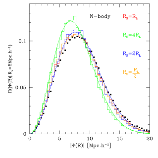
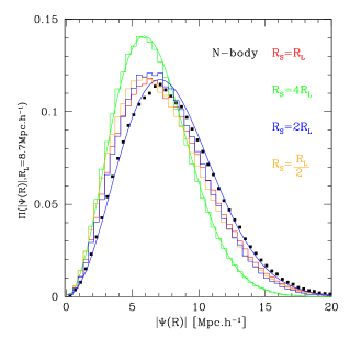
In Fig.(1), we show the measured PDF of $\Psi$ (black squares) for two different masses of halos: the upper panel corresponds to halos with Lagrangian radii $R_{L}=5\,h^{-1}$ Mpc ($M=10^{13.6}h^{-1}M_{\odot}$) while the lower panel corresponds to halos with Lagrangian radius $R_{L}=8.7\,h^{-1}$ Mpc ($M=10^{14.3}h^{-1}M_{\odot}$). As we can see, the mean displacement is not strongly sensitive to the mass of the proto-halos (varying by only $\sim 15\%$). However, the variance of the absolute displacement is reduced for large halos. Physically, this is because larger proto-halos are less sensitive to the external shear field which contributes to the overall dynamics. In Fig.(1), we can also see the prediction of Eq.(7) (plotted as histograms) using different smoothing scales $R_{S}$ (see legend) when measuring the average peculiar velocities. For $R_{S}\leq 2R_{L}$, the absolute displacement predicted by Eq.(7) is approximately independent of $R_{S}$. For $R_{S}=4R_{L}$, we begin to smooth out relevant density fluctuations and hence underestimate the absolute displacement. In the limit $R_{S}>>R_{L}$, the analytical pdf of $\Psi$ is given by a Maxwell-Boltzmann distribution (Koppetal2015 ),

$$\Pi(\Psi,\sigma_{\Psi})=\sqrt{\dfrac{2}{\pi}}\left(\frac{\sqrt{3}}{\sigma_{\Psi}}\right)^{3}\Psi^{2}\exp{\left[-\frac{3\Psi^{2}}{2\sigma^{2}_{\Psi}}\right]}$$ (8)

where the variance is

$$\sigma^{2}_{\Psi}(R)=\frac{1}{2\pi^{2}}\int\tilde{W}^{2}(R,k)\,P_{L}(k,z)\,dk.$$ (9)

The Fourier transform of the filter function $\tilde{W}(R,k)$ is chosen to be the Fourier transform of a top-hat filter in real space. In Fig.(1) we can see this analytical prediction for $R=4R_{L}$ and $R=2R_{L}$ (solid lines). For $R=4R_{L}$ the analytic prediction of Eq.(8) matches the Zel’dovitch prediction of Eq.(7) with $R_{S}=4R_{L}$ (comparing the green solid line and green histogram). For smaller smoothing scales ($R=2R_{L}$), the regime $R>>R_{L}$ is no longer satisfied and we start observing deviations between Eq.(8) and Eq.(7) (comparing the blue solid line and blue histogram). Interestingly, we observe that Eq.(8) qualitatively follows the trend for the absolute displacement of proto-halos (black squares) once we use $R=2R_{L}$. This observation could be used to model the clustering of halos with high accuracy, although this goes beyond the scope of this paper.

Figure 2: Standard deviation of the difference between the $x$-component of the exact displacement and the ZA Eq.(7), as a function of the ratio of the smoothing length and Lagrangian size of the halos, $R_{S}/R_{L}$. The red, black and blue crosses correspond to halo masses $10^{12.5}$, $10^{13.0}$ and $10^{14.3}h^{-1}M_{\odot}$.

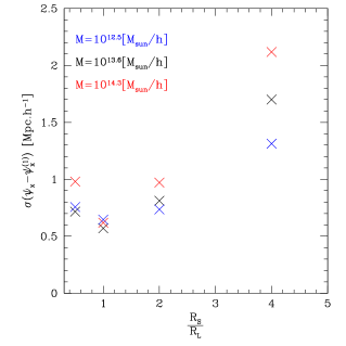
Second, we consider the dispersion between the exact and estimated displacements. For each component $i$, the PDF of $\Psi_{i}-\Psi^{(1)}_{i}$ follows a Gaussian distribution with a mean value equal to zero. In Fig.2 we can see the standard deviation of the difference between the exact and the Zel’dovitch prediction (Eq.(7)) of $\Psi_{x}$, for halo masses $10^{12.5}$, $10^{13.0}$ and $10^{14.3}h^{-1}M_{\odot}$, as a function of the smoothing length $R_{S}$ (similar results are obtained for $\Psi_{y}$ and $\Psi_{z}$). Independently of the proto-halo masses, the optimal smoothing scale to predict the final position of halos is $R_{S}=R_{L}$. At this scale $\Psi$ can be determined with an accuracy of $\sim 0.5\,h^{-1}$ Mpc, a few per cent of the mean displacement. This is an impressive result considering that we only use the ZA. It implies that if we can identify proto-halos in the initial matter density field, we can predict their clustering at $z=0$ with high accuracy in a very short time.

Figure 3: Standard deviation of the difference between the exact displacement and that predicted by Eq.(2,3) with $R_{S}=R_{L}$ in different environments. Colors represent different environments. The black square corresponds to the average density around halos $\bar{\delta}(R_{S}=R_{L})$. The blue, red and orange squares correspond to environments with local overdensity $\delta=\{\bar{\delta}-\sigma_{\delta},\bar{\delta}+\sigma_{\delta},\bar{\delta}+2\sigma_{\delta}\}$ respectively, where $\bar{\delta}$ is the mean overdensity and $\sigma_{\delta}$ is the standard deviation of the overdensity distribution amongst the halos.

Figure 4: Standard deviation of the difference between the $x$-component of the exact displacement, and the ZA computed using the $z=0$ density field using Eq.(2,3), as a function of the smoothing length $R_{S}$ and the type of filter used.

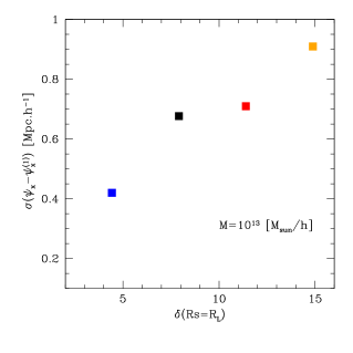
Finally, we test how sensitive the ZA (Eq.(7)) is to the local environment. Each environment is defined by the number density of halos inside a sphere of radius $R_{S}$. We divide the halos into environment bins by considering the probability density function for the number of halos at $z=0$ within $R_{S}=R_{L}$, in particular the mean $\bar{\delta}$ and standard deviation $\sigma_{\delta}$ of this distribution. We then define 4 different environments corresponding to halos with surrounding densities $\delta=\{\bar{\delta}-\sigma_{\delta},\bar{\delta},\bar{\delta}+\sigma_{\delta},\bar{\delta}+2\sigma_{\delta}\}$.

In Fig.(3) we can see the standard deviation between the true value and the ZA prediction of $\Psi_{x}$ (with $R_{S}=R_{L}$), as function of the surrounding number density of halos ($\delta(R_{S})$), considering halos with mass $M=10^{13}\,h^{-1}M_{\odot}$, which is equivalent to $R_{L}\sim 3\,h^{-1}$ Mpc. The black square corresponds to the mean overdensity environment. As we can see, the accuracy of the ZA prediction is sensitive to the environment. For overdense environments, the ZA prediction becomes less accurate compared to underdense environments. This suggests that the displacement field of proto-halos contains non-linear information that can not be encapsulated in the simple ZA. An extension of this work would be to investigate if the sensitivity to the smoothing scale and environment depends on cosmology.

In the next section, we will repeat this exercise, comparing the displacements reconstructed using the halo distribution at $z=0$ to evaluate the density contrast in Eq.(3), to the exact displacements.

III Performance of density-field reconstruction

III.1 Displacement prediction from density-field reconstruction

We first describe how we predict the displacement field from the $z=0$ halo distribution using the technique of density-field reconstruction. Dividing the volume into a 3D grid, we first estimated the halo overdensity distribution at each grid point, using a particular filter (Gaussian or top-hat) and smoothing scale. We then convert the halo overdensity $\delta_{h}(R_{S})$ to a matter overdensity $\delta_{m}(R_{S})=\delta_{h}(R_{S})/b$ assuming a linear bias factor $b$, which we determine by comparing the amplitude of the large-scale halo power spectrum to the linear-theory power spectrum used to generate the simulation. This allows us to solve Eq.(3) using Fast Fourier Transform methods, and hence determine the displacement field $-\mathbf{\Psi}(R_{S})$ via Eq.(2).

III.2 Dependence on smoothing scale and filter

Figure 5: Standard deviation of the difference between the $x$-component of the exact displacement, and that computed using the $z=0$ density field using Eq.(2,3), as a function of the smoothing length $R_{S}$ using a Gaussian filter. Black squares show the first-order (ZA) prediction while black crosses show the prediction including the 2LPT correction.

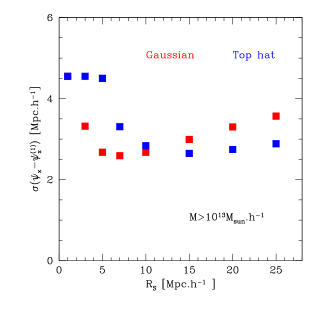
Considering only the first order of $\mathbf{\Psi}$ in Eq.(2,3), we used several smoothing scales in the range $0<R_{S}<25\,h^{-1}$ Mpc for halos with a mass $M>10^{13}h^{-1}M_{\odot}$, typical of Luminous Red Galaxies probed by large-scale structure surveys such as the Baryon Oscillation Spectroscopic Survey (Andersonetal2014 ). We used both a top-hat filter and a Gaussian filter, and we measured the error made in the Zel’dovitch prediction compared to the exact values for each component as a standard deviation $\sigma(\psi_{i}^{(1)}-\psi_{i})$. The result for the $x$-axis is shown in Fig.(4), other axes produced similar results. We find that there is again an optimal smoothing scale which depends on the filter function. The optimal performance of both filters leads to a residual error $\sigma\sim 2.5\,h^{-1}$ Mpc, around 5 times poorer than the determination based on the initial proto-velocities.

For small smoothing scales the performance of the reconstruction method becomes worse, since the number of neighbours becomes too small to reconstruct the density field with sufficient accuracy. Furthermore, the higher order correction in Eq.(2) becomes non-negligible when $R_{S}\rightarrow 0$. For large smoothing scales, the degradation from the optimal performance is a slow function of $R_{S}$, consistent with the displacement being generated by large-wavelength modes that may be successfully recovered even in the presence of significant smoothing (Eisensteinetal.2007 ). These effects are illustrated in Fig.(5). Using a Gaussian filter we show the error made in the 1st-order (black squares) and 2LPT (black crosses) predictions for different smoothing scales. The 2nd-order correction leads to a $\sim 2\%$ improvement for $R_{S}\sim 8h^{-1}$ Mpc and a $\sim 12\%$ improvement for $R_{S}\sim 5h^{-1}$ Mpc. In the next section we will emphasize the connection between this result and the local environment.

Overall, the choice of filter (Gaussian vs. top-hat) does not affect the performance of the displacement reconstruction at first-order LPT, once we choose the optimal smoothing scale (see Fig.(4)). Therefore in what follows we will restrict our analysis to a Gaussian filter.

III.3 Dependence on local environment

Figure 6: Standard deviation of the difference between the exact displacement and that predicted by Eq.(2,3) based on the $z=0$ halo density field. The squares show the first order implementation of Eq.(2,3) while the crosses implement the second order correction. Colors represent different environments defined in the text (from bottom to top: E1, E2, E3, E4 and E5). For each color we choose 3 smoothing scales (from left to right: $R_{S}=10,7.5,5\,h^{-1}$ Mpc.

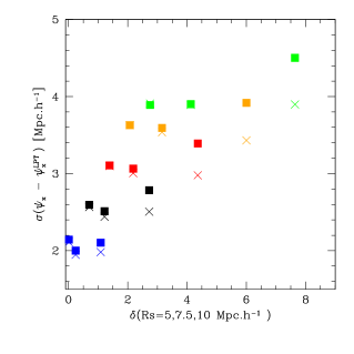
In this Section we investigate how the accuracy of the reconstructed displacement field depends on the local environment of each halo. Given a smoothing scale $R_{S}$, we can compute the number of neighbours for each halo and therefore estimate the local density contrast. We used the mean local density around halos $\bar{\delta}$, and the standard deviation $\sigma_{\delta}$, to define five bins in environment E1, E2, E3, E4 and E5 with central values $\delta=\left\{\bar{\delta}-\sigma_{\delta},\bar{\delta},\bar{\delta}+\sigma_{\delta},\bar{\delta}+2\sigma_{\delta},\bar{\delta}+3\sigma_{\delta}\right\}$. For each local environment we measured the error in the reconstructed displacement at different smoothing scales.

In Fig.(6) we show the standard deviation of the difference between the reconstructed and exact $\Psi_{x}$, as function of the surrounding smoothed halo density $\delta(R_{S})$. The blue, black, red, orange and green data points correspond respectively to environments E1, E2, E3, E4, and E5. For each environment we plot 3 different squares and 3 different crosses which correspond to three different smoothing scales $R_{S}=10,7.5,5\,h^{-1}$ Mpc, from left to right. The squares correspond to the prediction of first-order LPT, while the crosses implement the second-order correction.

In agreement with Fig.(3), the accuracy of the prediction is highly sensitive to the environment. Furthermore, in Fig.(6) we can see the effect of the second-order correction. Unsurprisingly, if we choose a large smoothing scale (e.g. $10\,h^{-1}$ Mpc), the second order correction in Eq.(2) is negligible. For a smaller smoothing scale (e.g. $R_{S}=5\,h^{-1}$ Mpc), the second-order correction becomes more important. In fact, the second-order correction contains a term proportional to $\delta^{2}(R_{S})$ and for small values of $R_{S}$ the average local density around halos increases ($\bar{\delta}(R_{S}=10)\sim 0.8$, $\bar{\delta}(R_{S}=5)\sim 2.8$). However we can observe that even for $R_{S}=5\,h^{-1}$ Mpc, the improvement in the residual from the second-order correction is less significant than the difference in residual between E1 and E2. This suggests that the displacement contains non-linear information that can not be described by deterministic corrections.

Finally, for dense environments (e.g $\delta>\bar{\delta}$), a smaller smoothing scale leads to a better reconstruction of the final halo position predicted by the 2LPT approximation (Eq.3). For halos in a region with the mean density or below, reducing the smoothing scale does not particularly improve the accuracy of the displacement field. This convergence of the optimal smoothing scale toward $R_{S}\rightarrow R_{L}$ shows the limits of the reconstruction method. Reconstruction applied at $z=0$ on the non-linear halo density field is not equivalent to predicting the final position of halos from the initial conditions.

III.4 Dependence on redshift and halo mass

Figure 7: Same as Fig.(6), for halos at redshift $z=1$ in the mass range $M>10^{13}h^{-1}M_{\odot}$.

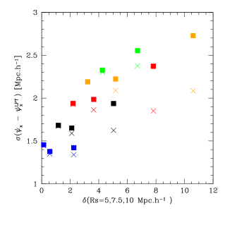
We repeated the previous analysis at redshift $z=1$. Fig.(7) displays these results in the same format as Fig.(6). As before, for large values of the smoothing (e.g. $R_{S}=10\,h^{-1}$ Mpc), the second-order correction is negligible, while it becomes important for smaller smoothing scales when the local density around halos is high. In this case, choosing a smaller smoothing scale (e.g. $R_{S}=5\,h^{-1}$ Mpc) and adding the second-order correction to Eq.(3) gives a better description of the displacement field (Eq.(2)). We note that at $z=1$ the second-order correction is more important than at $z=0$. This is due to the choice of halos we consider. At $z=1$, halos with $M>10^{13}h^{-1}M_{\odot}$ are more biased and belong to exponential tail of the halo mass function (AWWR, ). Hence the local overdensity around those halos is larger, leading to a higher second-order correction of the displacement field.

Figure 8: Same as Fig.(6), for halos at redshift $z=1$ in the mass range $M>10^{12.5}h^{-1}M_{\odot}$.

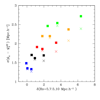
For halos with mass $M>10^{12.5}h^{-1}M_{\odot}$ at $z=1$, the error in the displacement is shown in Fig.(8). For $R_{S}=10\,h^{-1}$ Mpc, the second-order correction is negligible and the error in the displacement is similar to that found for halos with $M>10^{13}h^{-1}M_{\odot}$ at $z=0$. For smaller smoothing scales, the second-order correction becomes more important.

Overall, at $z=1$ the analytic approximations for the displacements (Eq.(2)) are in better agreement with the true displacements we measure in the simulations, by a factor which depends on the environment. For instance at the average density (E3, black cross), the standard deviation of the residual is $\sim 2.5\,h^{-1}$ Mpc at $z=0$ and $\sim 1.6\,h^{-1}$ Mpc at $z=1$.

IV Effect on the baryon acoustic correlation function peak

In this Section we study how the reconstruction of the baryon acoustic peak depends on the accuracy with which the displacement field can be determined. In particular, we investigate if the “sharpness” of the reconstructed acoustic peak depends on local overdensity, and if this effect may be used to obtain improved accuracy in the resulting standard ruler measurement.

IV.1 The WizCOLA N-body simulations

In order to obtain an accurate covariance matrix for our BAO fits, we require a much larger suite of N-body simulations than we used in the previous sections. We therefore analyzed the “WizCOLA” simulations (Kodaetal2015 ), which were produced in order to extend the Comoving Lagrangian Acceleration (COLA) technique (Tassev2013, ) to lower-mass haloes to enable reconstruction of the baryon acoustic peak in the WiggleZ Dark Energy Survey (Kazinetal2014 ). The simulations are generated within a $600\,h^{-1}$ Mpc box using the “WMAP5” cosmological model. In particular, we used 1000 halo catalogues output at $z=0$ in real-space, using halos with mass $M>10^{13}\,h^{-1}M_{\odot}$ as above, which yields a catalogue with number density $\sim 5\times 10^{-4}\,h^{3}$ Mpc^-3, characteristic of current and future large-scale structure surveys at high redshift.

We applied the density-field reconstruction method to these simulation boxes using standard methods described by, e.g. Padmanabhanetal2012 ; Andersonetal2014 ; Kazinetal2014 . The process involves applying the displacements to both the data and a set of random points, which we generated uniformly within each simulation box with a number density 10 times greater than that of the data itself. The post-reconstruction correlation function is then measured using the displaced data and random points. When determining the displacement field we assumed a linear bias factor $b\approx 1.4$, fixed using the large-scale halo power spectrum.

IV.2 The correlation functions measured in different environments

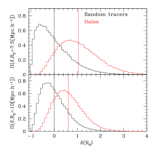
As in section III.3, we divided the simulation into different density regimes by smoothing the density field traced by the halos. Fig.(9) displays the probability density function $\Pi(\delta,R_{S})$ of the local overdensity $\delta$ around halos (red histogram) and random tracers (black histogram) at $z=0$. The top panel is for a smoothing scale $R_{S}=7.5\,h^{-1}$ Mpc, while the lower panel shows the PDF for $R_{S}=10\,h^{-1}$ Mpc. The vertical lines show the mean of the two distributions; for random tracers the mean is always zero, while for halos the mean of the distribution increases for smaller smoothing scales due to clustering.

We split our sample into different environment bins using the local density around halos. For the purposes of this section we use 5 different environments. We defined the bin divisions by measuring the mean $\overline{\delta}$ and standard deviation $\sigma_{\delta}$ of the density values for each halo. In this case, environment $E_{3}$ corresponds to the average density and the central density values of the other environments are set using

$$\delta=\bar{\delta}+(i-3)\sigma_{\delta}.$$ (10)

We also tested defining the bins based on the local density around random tracers, which produced qualitatively similar results.

We measured auto- and cross-correlation functions between different environments using the Landy-Szalay estimator (LandySzalay1993 ). The cross-correlation function between environments $(E_{i},E_{j})$ is therefore

$$\xi_{ij}=\frac{DD_{ij}}{RR_{ij}}\frac{n_{Ri}n_{Rj}}{n_{Di}n_{Dj}}-\frac{DR_{ij}}{RR_{ij}}\frac{n_{Ri}}{n_{Di}}-\frac{DR_{ji}}{RR_{ij}}\frac{n_{Rj}}{n_{Dj}}+1$$ (11)

where $DD_{ij}$ are the pair counts of halos between environments $(i,j)$ $n_{Di}$ is the total number of halos in the environment $i$, $RR_{ij}$ are the pair counts of random tracers, $DR_{ij}$ the cross-pair counts, and $n_{Ri}$ the total number of random tracers in environment $i$.

We determined the covariance matrix of the cross-correlation function between two separation bins $(r_{k},r_{l})$ by averaging over the ensemble of N-body realizations:

$$C_{k,l}=\langle\xi_{ij}(k)\,\xi_{ij}(l)\rangle-\langle\xi_{ij}(k)\rangle\langle\xi_{ij}(l)\rangle$$ (12)

The error in the measurement of $\xi_{ij}(r_{k})$ is then $\sqrt{C_{k,k}}$.

Figure 9: The probability density function for the smoothed overdensity $\delta$ around halos and random tracers measured at $z=0$. The top panel shows this PDF for $R_{S}=7.5\,h^{-1}$ Mpc, while the lower panel is for $R_{S}=10\,h^{-1}$ Mpc.

Figure 10: The auto-correlation functions measured in the different environments, from bottom to top the measurements correspond to $\xi_{11},\xi_{55},\xi_{44},\xi_{33},\xi_{22}$. We use $R_{S}=10\,h^{-1}$ Mpc for the smoothing scale.

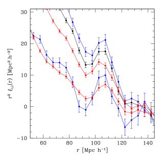
In Fig.(10) we plot the auto-correlation functions $\xi_{ii}(r)$ measured in the 5 different environments after reconstruction. The black line (and dots) correspond to $E_{3}$, the red lines (and dots) correspond to overdense environments $E_{4},E_{5}$ while the blue lines (and dots) are for underdense environments $E_{1},E_{2}$. In order to produce a clearer visualization for the purposes of this plot, we stacked the simulation boxes in groups of 10, such that the error in the measurements is then determined from 100 realizations of 10 stacked boxes. Fig.(10) clearly displays a hierarchy where the baryon acoustic peak is sharper for the underdense regions and becomes more blurred for the high density regions. Interestingly, the most under-dense environment produces a “bell shape” around the acoustic peak. The cross-correlation functions display behaviour intermediate between the corresponding auto-correlation functions.

Figure 11: Correlation functions measured in the different environments for $R_{S}=10\,h^{-1}$ Mpc before (dashed lines) and after reconstruction (solid lines and dots). From bottom to top the measurements correspond to environments $E_{1},E_{5},E_{4},E_{3},E_{2}$.

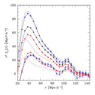
In order to further understand how the correlation functions $\xi_{ij}$ are affected by the reconstruction method, we plot in Fig.(11) the full correlation function before and after reconstruction. We see that reconstruction uniformly improves the sharpness of the acoustic peak in all environments.

The increased sharpness of the post-reconstruction baryon acoustic peak in underdense environments could potentially be used to improve the accuracy of the standard ruler by upweighting those environments. However, the fluctuating weight could also serve to increase the covariance in our measurements. We now explore the trade-off between these effects. We note that using density-dependent weights will always result in a biased estimator for the underlying correlation function. However, given that the amplitude and shape of the correlation function are marginalized over in standard methods of fitting the preferred scale, this bias is not necessarily problematic if the acoustic peak itself is not shifted.

IV.3 Total correlation function and new estimators

The total correlation function $\xi$ can be expressed as a function of the environmental correlation functions Eq.(11). We begin with the Landy-Szalay estimator for $\xi$,

$$\xi=\frac{DD}{RR}\frac{n_{R}^{2}}{n_{D}^{2}}-2\frac{DR}{RR}\frac{n_{R}^{2}}{n_{DR}^{2}}+1$$ (13)

where $DD$, $RR$ and $DR$ are the total pair counts (halo-halo, random-random tracer, halo-random tracer). The total number of halos ($n_{D}$), random tracers ($n_{R}$) and cross-product ($n_{DR}$) appearing in this equation satisfy $n_{D}^{2}=\sum_{ij}n_{Di}n_{Dj}$, $n_{R}^{2}=\sum_{ij}n_{Ri}n_{Rj}$ and $n_{DR}^{2}=\sum_{ij}n_{Di}n_{Rj}$, where the sum is over all environments (and is written in this manner to allow us to generalize the relation as developed below). The conservation of the total number of pairs can be expressed as

$$DD=\sum_{i,j}DD_{ij}$$ (14)

Substituting Eq.(14) into Eq.(13), we can express $\xi$ as function of the $\xi_{ij}$ as

$$\xi=\frac{n_{R}^{2}}{n_{D}^{2}}\frac{1}{RR}\sum_{i,j}DD_{ij}-2\frac{DR}{RR}\frac{n_{R}^{2}}{n_{DR}^{2}}+1$$ (15)

where

$$\begin{split}&\sum_{i,j}DD_{ij}\equiv RR_{ij}\frac{n_{Di}n_{Dj}}{n_{Ri}n_{Rj}}\left(\xi_{ij}-1\right)-\\ &DR_{ij}\frac{n_{Di}}{n_{Ri}}-DR_{ji}\frac{n_{Dj}}{n_{Rj}}.\end{split}$$ (16)

Hence we have obtained an expression for the total correlation function in terms of $\xi_{ij}$.

IV.3.1 Illustrative example

As a first illustration of the effect of assigning a different weight to different environments, we re-write $\xi_{ij}$ in Eq.(15) as $w_{ij}\,\xi_{ij}$, where $w_{ij}\equiv\sqrt{w_{i}w_{j}}$ is the weight assigned to each cross-correlation function in terms of weights $w_{i}$ defined for each environment $E_{i}$. In the case where $w_{i}=1$, we recover the original correlation function. For the purposes of this example we consider a simpler split into 3 environments.

Figure 12: The linear correlation function (blue dashed line) and measured correlation function at $z=0$ (orange dashed line). The standard reconstructed correlation function is shown by the black line, while the blue and red lines are particular cases of our new estimate for the reconstructed correlation functions weighting by environment.

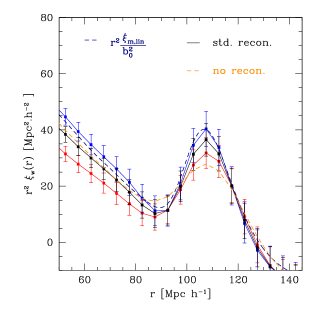
In Fig.(12), we show the linear matter correlation function rescaled by the linear bias (blue dashed line) and the non-linear matter power spectrum measured in the simulations (orange dashed line). The black line (and dots) shows the reconstructed correlation function using $R_{S}=10\,h^{-1}$ Mpc with no weighting. For comparison we plot the weighted correlation function for two special cases (blue and red), where we choose $w_{1}=2,w_{2}=2,w_{3}=0.5$ for the blue line (upweighting low-density environments) and $w_{1}=0,w_{2}=0.5,w_{3}=2$ for the red line (upweighting high-density environments). We can see that weighting the underdense environment ($E_{1}$) more than the overdense environment ($E_{3}$) allows us to recover the linear (sharpest) amplitude of the BAO peak.

IV.3.2 General linear weighting

We now construct a general estimator for the weighted correlation function, insensitive to the absolute value of the weights, as

$$\xi_{w}=\frac{\sum_{ij}\left(w_{ij}\,\xi_{ij}\,RR_{ij}\,\alpha_{ij}+\beta_{ij}\right)}{\sum_{ij}w_{ij}\,RR_{ij}}$$ (17)

where

$$\alpha_{ij}=\left(\frac{n_{R}}{n_{D}}\right)^{2}\frac{n_{Di}\,n_{Dj}}{n_{Ri}\,n_{Rj}},$$ (18)

and

$$\begin{split}&\beta_{ij}=\left(\frac{n_{R}}{n_{D}}\right)^{2}\bigg{[}\Big{(}\frac{n_{Dj}}{n_{Rj}}-\frac{n_{D}^{2}}{n_{DR}}\Big{)}DR_{ij}+\\ &\Big{(}\frac{n_{Di}}{n_{Ri}}-\frac{n_{D}^{2}}{n_{DR}}\Big{)}DR_{ji}+\left(\frac{n_{Di}\,n_{Dj}}{n_{Ri}\,n_{Rj}}-\frac{n_{D}^{2}}{n_{R}^{2}}\right)RR_{ij}\bigg{]}\end{split}$$ (19)

and we re-defined $n_{D}^{2}=\sum_{ij}w_{ij}n_{Di}n_{Dj}$, $n_{R}^{2}=\sum_{ij}w_{ij}n_{Ri}n_{Rj}$ and $n_{DR}^{2}=\sum_{ij}w_{ij}n_{Di}n_{Rj}$. This new estimator has the following desirable properties: $\xi_{w}=\xi$ for $w_{ij}={\rm constant}$, and $\xi_{w}=\xi_{kl}$ when $w_{ij}=\delta_{ik}\delta_{jl}$.

To assign a value for each $w_{ij}=\sqrt{w_{i}w_{j}}$ in Eq.(17) we used the following parametrization:

$$w_{i}\equiv 1+x\left(\frac{i-\bar{i}}{i_{\rm max}-\bar{i}}\right)$$ (20)

where $\bar{i}$ corresponds to the environment for which the local density $\delta(R_{S})=\bar{\delta}$, $i_{\rm max}=2\bar{i}-i_{\rm min}$ is the highest density environment, and $x$ is a variable that varies in the range $x=\left[-1,1\right]$ such that for $x=-1$, the lowest-density environment is weighted with the highest amplitude $w_{i_{\rm min}}=2$ and the highest environment is weighted with $w_{i_{\rm max}}=0$.

Figure 13: The linear correlation function (blue dashed line) and measured unweighted correlation function at $z=0$ (orange dashed line). The solid lines show the weighted correlation function for $x=-1,-0.5,0,0.5,1,$ which correspond to the blue, dark blue, black, orange and red lines, respectively. We do not show the errors in the measurement for clarity of the Figure.

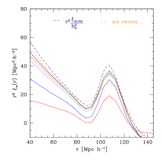
In Fig.(13) we can see the resulting weighted correlation functions for various values of $x$, as well as the linear and non-linear correlation functions. We used 5 different environments and $R_{S}=10\,h^{-1}$ Mpc. We observe that the hierarchy of the $\xi_{w}$ is not as simple as we show in Fig.(12). With this parametrization, the standard reconstruction (black line, $x=0$) is closer to the linear correlation function than the measurement obtained assigning higher weight to the underdense environments (blue and light-blue lines) owing to the amplitude bias introduced by the weighting. However, the sharpness of the acoustic peak is nonetheless increased by such a weighting scheme. In the next section we consider the implications for the recovered standard ruler scale.

IV.4 Baryon acoustic peak fitting

In order to determine the accuracy of the recovered distance scale, we fit a simple baryon acoustic peak model to the galaxy correlation functions measured from each N-body realization, using the distribution of measurements across the realizations as the covariance matrix. Our fiducial correlation function model is based on a Fourier-transform of a model linear power spectrum $P(k)$:

$$\xi_{\rm fid}(s)=\frac{1}{2\pi^{2}}\int dk\,k^{2}\,P(k)\,\left[\frac{\sin{(ks)}}{ks}\right].$$ (21)

We constructed the model power spectrum using a transfer function from the Eisenstein & Hu (1998) fitting formulae, assuming the fiducial cosmological parameters of the WiZCOLA simulations. We then fit for the scale distortion parameter $\alpha$, marginalizing over a normalization factor $b^{2}$:

$$\xi_{\rm mod}(s)=b^{2}\,\xi_{\rm fid}(\alpha s)$$ (22)

This approximate model is adequate for our purposes of exploring the relative accuracy of determining $\alpha$; we verified that a series of model extensions, such as using a model power spectrum from CAMB, or marginalizing over an additive scale-free polynomial or a free damping parameter, or using the mock mean correlation function as a template, did not qualitatively change our conclusions.

We quantified the standard ruler performance by the standard deviation of the best-fitting values of $\alpha$ across the realizations, which we denote by $\sigma_{\alpha}$. For this particular test we used the 1000 single-box COLA realizations and 12 environments, checking that our conclusions were not sensitive to these choices.

In order to test any improvement brought by the new concepts developed in the previous sections, we defined as a reference level the results obtained by a standard reconstruction method using the Zel’dovitch approximation, smoothing length $R_{S}=10\,h^{-1}$ Mpc, and no weighting ($x=0$). Similar assumptions are used in standard implementations such as ((Padmanabhanetal2012, ; Andersonetal2014, ; Kazinetal2014, )). Using the measurements of $\sigma_{\alpha}$, we computed the relative difference $\Delta\sigma_{\alpha}$ between the reference model and the results obtained (a) changing the smoothing length, (b) adding the 2LPT correction and (c) introducing weighting of environments as a function of $x$.

In Fig.(14) we display our results for this analysis, in the form of the relative difference $\Delta\sigma_{\alpha}$ as function of the weighting parameter $x$ defined by Eq.(20). The solid line uses the reconstruction method with the Zel’dovitch approximation and $R_{S}=10\,h^{-1}$ Mpc, the blue short dashed line shows the result for 2LPT and $R_{S}=7.5\,h^{-1}$ Mpc while the red dashed line shows 2LPT and $R_{S}=5\,h^{-1}$ Mpc.

Figure 14: The accuracy of the recovery of the standard ruler after density-field reconstruction, relative to a reference implementation, as a function of the parameter $x$ in Eq.(20) which controls the relative weight assigned to underdense and overdense regions. The reference case is the ZA with $R_{S}=10\,h^{-1}$ Mpc and no weighting.

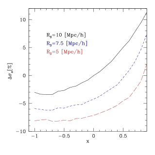
We find that the environmental-dependent weighting produces a small but measurable improvement in $\sigma_{\alpha}$ ($\sim 3\%$), with best performance usually produced in the range $-1<x<-0.5$. The implementation of 2LPT for computing the displacement field also produces a benefit as judged by $\sigma_{\alpha}$, such that the total improvement is $\sim 8\%$.

V Discussion and conclusion

We summarize the conclusions of our study as follows:

• The displacement of proto-halos can be predicted with high accuracy by the ZA using their peculiar velocities. In this case, Eq.(7) evaluated at $R_{S}=R_{L}$ provides a very good description of the displacement field with accuracy $\sigma_{\Psi}\sim 0.5\,h^{-1}$ Mpc, independently of the halo masses. The choice of the smoothing scale is important, since there is a unique scale for which the approximation gives the best agreement with the exact final positions of the halos. The error in each component of $\mathbf{\Psi}$ follows a Gaussian distribution centered on zero with a variance sensitive to the smoothing scale and the environment of the halos.

• When reconstruction of the displacement field is performed using the $z=0$ halo distribution in real space, we likewise find that the accuracy depends significantly on the smoothing scale and environment. We extended the ZA to 2LPT and established a link between the error in predicting the displacement field and the local density around halos.

• Based on this result, we showed that after applying reconstruction, the baryon acoustic peak is sharper in the correlation function of low-density environments. We hence built a new estimator of the correlation function, constructed by weighting a set of auto- and cross-correlation functions measured between different environments.

• Fitting a BAO model to the results, we found a small but measurable improvement of $\sim 8\%$ in determining the standard ruler scale through a combination of using 2LPT to find the displacement field and weighting the environmental correlation functions. Further improvements may be possible using more sophisticated weighting schemes.

The fact that the reconstruction of the displacement field using the halo density distribution at $z=0$ is $\sim 5$ times less accurate than the ZA applied to the initial velocities of proto-halos (independently of the orders considered in the LPT approximation) implies that the measurement of the error $\sigma(\psi_{i}-\psi_{i}^{(1)})$ contains non-linear information which could potentially be sensitive to different cosmological models, especially in high-density environments. The evolution in time of the environmental correlation functions should carry this non-linear information and can be use to test non-standard cosmologies.

For instance in Fig.(11), the correlation function before reconstruction in high-density environments has a smeared BAO peak compared to that of the lowest density environment. The ratio of the BAO peak widths in those two environments should be directly proportional to the degree of late time non-linear interactions. For non-standard cosmologies, this ratio might be different (e.g., fewer non-linear interactions for early dark energy models). We will investigate these topics further in future work.

VI Acknowledgments

We warmly thank Y. Rasera for providing easy access to the DEUS simulations(DEUSweb, ). We are also grateful to Jun Koda for generating the WizCOLA simulation suite used in this investigation. Part of this research was conducted by the Australian Research Council Centre of Excellence for All-sky Astrophysics (CAASTRO), through project number CE110001020. We also acknowledge support from the DIM ACAV of the Region Ile-de-France.