The spectral gap and the dynamical critical exponent of an exact solvable probabilistic cellular automaton

Abstract

We obtained the exact solution of a probabilistic cellular automaton related to the diagonal-to-diagonal transfer matrix of the six-vertex model on a square lattice. The model describes the flow of ants (or particles), traveling on an one-dimensional lattice whose sites are small craters containing sleeping or awake ants (two kinds of particles). We found the Bethe ansatz equations and the spectral gap for the time-evolution operator of the cellular automaton. From the spectral gap we show that in the asymmetric case it belongs to the Kardar-Parisi-Zhang (KPZ) universality class, exhibiting a dynamical critical exponent value $z=\frac{3}{2}$. This result is also obtained from a direct Monte Carlo simulation, by evaluating the lattice-size dependence of the decay time to the stationary state.

I Introduction

The six-vertex model was introduced in 1931 by Pauling in order to explain the residual entropy of the ice at zero temperature. The model turns out to be of great interest for physicists and mathematicians of many-body systems due to its exact integrability lieb1 . The row-to-row transfer matrix of the six-vertex model is the generating function for an infinite set of commuting non-trivial charges in involution tarasov . The anisotropic Heisenberg chain, or the so called XXZ quantum chain, is one of these conserved charges. Actually, a quantum system is integrable whenever its Hamiltonian belongs to an infinite set of commuting operators. The exact integrability of the XXZ quantum chain is then a consequence of the infinite number of commuting charges generated by the six-vertex model. For this reason the six-vertex model is considered as a paradigm of exact integrability in statistical mechanics lieb ; sutherland-yang-yang ; baxter ; gaudin .

On the other hand, the representation of interacting stochastic particle dynamics in terms of quantum spin systems produced interesting and fruitful interchanges among the area of equilibrium and non-equilibrium statistical mechanics. The connection among these areas follows from the similarity between the master equation describing the time-fluctuations on non-equilibrium stochastic problems and the quantum fluctuations of equilibrium quantum spin chains lushi ; shu1 ; alcrit1 ; alcrit2 ; alcaraz1 ; stinch1 ; krebs1 ; shu2 ; mario1 ; spohn ; kim ; dasmar ; sasawada ; PRE ; der3 ; ligget ; BJP1 ; BJP2 ; schu-domb . The simplest example is the asymmetric diffusion of hard-core particles on the one dimensional lattice (see der3 ; ligget ; schu-domb for reviews), where the time fluctuations are governed by the time evolution operator that coincides with the exact integrable XXZ quantum chain in its ferromagnetically ordered regime.

An important consequence of the above mentioned mathematical connection between quantum chains and interacting stochastic problems is that, unlike the area of non-equilibrium interacting systems where very few models are fully solvable, there exists a huge family of quantum chains appearing in equilibrium problems that are integrable by the Bethe ansatz on its several formulations (see baxter ; revkore ; revessler ; revschlo for reviews). In these cases, the Bethe ansatz enable us to obtain exactly the complete spectrum of the master equation describing the time-fluctuations on the non-equilibrium stochastic problem. From the spectrum we can compute important properties of the system. As for example, the relaxation time to the stationary state which depends on the system size $L$. It satisfies a scaling relation $\tau_{L}\sim L^{z}$, where the dynamical exponent $z$ can be obtained from the finite-size dependence of the real part of spectral gap between of the two leading eigenvalues ruling the long time regime.

In addition, although less explored in the literature, there is also a non-trivial connection between the transfer matrix operator of two-dimensional vertex models in thermal equilibrium and the time evolution operator in discrete time Markov chains schu-domb . Examples of this connection are given by the six-vertex model. It describes a non-local parallel diffusion of hard-core particles spohn ; kim , and also the time-evolution operator of a two steps local cellular automaton describing a half-parallel dynamics of asymmetric diffusion of hard-core particles schu-domb ; KDN . Another application is given by the ten-vertex model introduced in 10vertex to describe a parallel dynamics of a traffic flow stochastic cellular automaton.

The connection of the KPZ dynamics with the row-to-row transfer matrix of the six-vertex model was first observed by Gwa and Spohn spohn . This result for the six-vertex model on a cylinder was confirmed by several works including the analytical computation from Bukman and Shore bukman . Furthermore, more recently a rigorous proof of the KPZ exponent was also obtained for the six-vertex model on a quadrant with parameters on the stochastic line by Borodin, Corwin and Gorin borodin . It is interesting also to mention that in halpin we can find a recent review of theoretical and experimental realizations of the KPZ dynamics.

In the present work we study a simple one-dimensional probabilistic cellular automaton related to the diagonal-to-diagonal transfer matrix of the six-vertex model. This model is inspired in the idea of Alcaraz and Bariev 10vertex and describes the flow of particles, ants, automobiles, or some other conserved quantity in a one-dimensional discrete chain. Despite the diagonal-to-diagonal six-vertex model being known to be solvable for quite a long time bariev-81 , to our knowledge the spectral gap for this model with Boltzmann weights associated to stochastic processes was not considered previously. In this work we calculate the spectral gap for this model and found that the associated probabilistic cellular automaton belongs to the Kardar-Parizi-Zhang (KPZ) universality class with a dynamical exponent $z=\frac{3}{2}$ KPZ .

The layout of this papers is as follows. In Section II we introduce the probabilist cellular automaton and show its correspondence with the row-to-row transfer matrix of the six vertex model. In section III we solve exactly the model using a matrix-product ansatz. In section IV we calculate numerically the spectral gap related to the highest eigenvalues of the time-evolution operator and obtain the dynamical critical exponent. In Section V we perform Monte Carlo simulations of the cellular automaton. Finally in section VI we conclude our paper with a summary of the main results.

II The stochastic cellular automaton and its connection with the exactly integrable six-vertex mode

The main ingredients of a cellular automaton are the associated configuration space and the dynamical rules defining its time evolution. The cellular automaton we consider is defined on a $L$-site chain where at each site we attach a variable that have four possible values, and the configuration space has then $4^{L}$ components. We can associate to the four possibilities of site occupation arbitrary objects. We chose here a simple formulation of the automation where the four possibilities corresponds to a vacant site, a site occupied by a single awake or sleeping ant, and a site double occupied by an awake and a sleepy ant. We should stress here that the probabilist cellular automaton we introduce is not intended to describe the realistic motion of real ants. For a more realistic motion we should also consider the effect of the pheromones in the ants motion, like e.g., in nishinari .

We consider $n$ ants traveling in a one dimensional tunnel that links $L$ small craters (sites), as shown in Fig. 1. On the craters the ants are on a sleeping or awake state. The craters are so small that at most it supports two ants and no more than one awake ant. The four possible occupations of a given crater are then: no ants, one ant (sleeping or awake) or two ants (one sleeping and another awake).

The dynamical rules are defined as follows. At a given unit of time all the ants travel to the next nearest crater to the left, or stay in the same crater. The travel happens with the following rules:

• If the ant is awake and alone in the crater it sleeps with probability $p$ or travels to the left crater with the probability $1-p$.

• If when the ant arrives to a crater it finds another ant sleeping, since they do not want a dispute (the connecting channels among the craters only allow a single traveling ant) with probability $1$ the ant travels to the left leaving the other one sleeping.

• If in a given crater there is a sleeping ant with a probability $q$ it awakes and travels to the left and with probability $1-q$ stay sleeping.

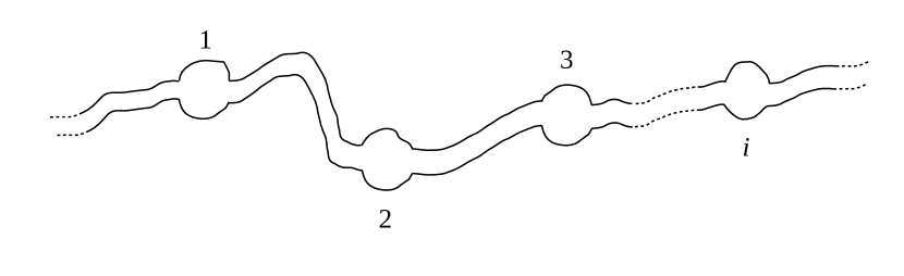
Figure 1: An illustrative example of a one dimensional set of tunnels connecting small craters.

The allowed motions, in a unit of time, can be represented by the arrow configurations of the six vertices shown in Fig. 2. The motions in Fig. 2 are from the top to the bottom of the figure. A vertical down arrow ($\downarrow$) represents an ant sleeping while the diagonal arrow ($\swarrow$) an awake ant, and lines with no arrows indicate the absence of ants. For simplicity, we consider periodic boundary condition. The conservation of the number of ants is then a consequence of the ice type rules defining the vertices, that demand an equal number of outgoing and incoming arrows in a given site.

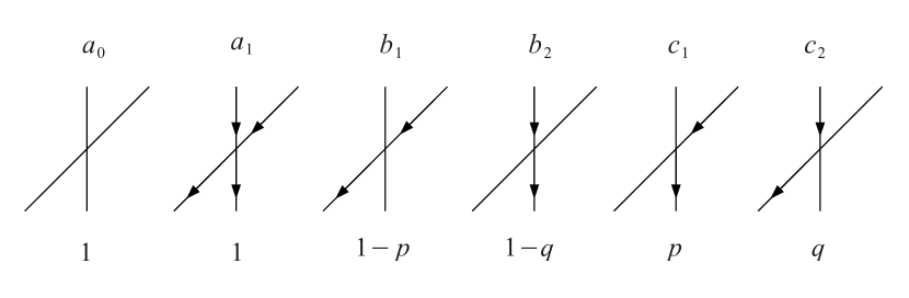
Figure 2: The fugacities of the six allowed vertex configurations of the equivalent vertex model. They correspond to the probabilities of motion in the probabilistic cellular automaton.

Let us denote as $\alpha_{j}$ the possible occupations of the crater $j$ by $\alpha_{j}=0,1,2$ and 3, that indicates that there is no ant, a sleeping ant, an awake ant, and a sleeping and awake and, respectively. The probability distribution $P(\{\alpha\},t)$ of finding the system in the state $|\{\alpha\}\rangle=|\alpha_{1},\alpha_{2},...,\alpha_{j},...,\alpha_{L}\rangle$ at time $t$ is given by the components of the probability vector.

$$|P(\{\alpha\},t)\rangle=\sum_{\{\alpha\}}P(\{\alpha\},t)|\{\alpha\}\rangle,$$ (1)

where the summation is performed over all possible configurations $\{\alpha\}=\{\alpha_{1},...,\alpha_{L}\}$ satisfying the ice type rules. The time evolution of the stochastic cellular automaton is given by the master equation:

$$|P(\{\alpha\},t+\Delta t)=T_{D-D}|P(\{\alpha\},t),$$ (2)

where the transition matrix $T_{D-D}$ corresponds to the diagonal-to-diagonal transfer matrix of a six-vertex model with fugacities $a_{0},a_{1},b_{1},b_{2},c_{1},c_{2}$ related, respectively, to the probabilities $1,1,1-p,1-q,p,q$ of the cellular automaton (see Fig. 2). The components $\langle\{\alpha\}|T_{D-D}|\{\alpha^{\prime}\}\rangle$ give the probability of motion from configuration $\{\alpha\}$ to $\{\alpha^{\prime}\}$ and are given by the product of the vertex fugacities connecting the configurations:

$$\langle\{\alpha\}|T_{D-D}|\{\alpha^{\prime}\}\rangle=a_{0}^{n_{0}}a_{1}^{n_{1}}b_{1}^{n_{2}}b_{2}^{n_{3}}c_{1}^{n_{4}}c_{2}^{n_{5}},$$ (3)

where $n_{0},n_{1},n_{2},n_{3},n_{4},n_{5}$ are the numbers of vertices with fugacities $a_{0},a_{1},b_{1},b_{2},c_{1},c_{2}$, respectively (see Fig. 3).

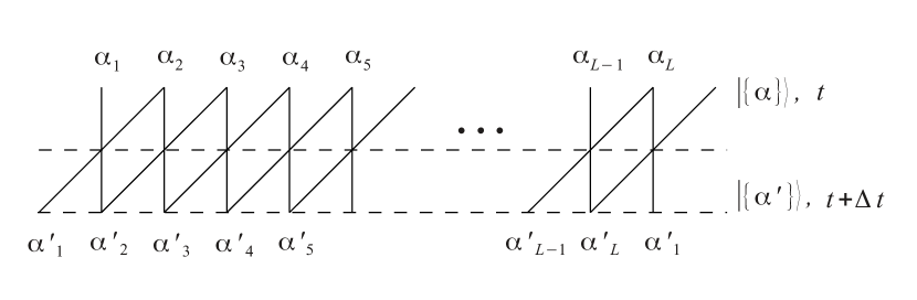
Figure 3: Pictoric representation of the diagonal-to-diagonal transfer matrix. The variables $\alpha_{j}$ and $\alpha^{\prime}_{j}$ specify the possible arrow configurations at site position $j$ at times $t$ and $t+\Delta t$, respectively.

The spectral properties of the six-vertex model are characterized by the parameter baxter :

$$\Delta=\frac{b_{1}b_{2}-c_{1}c_{2}+a_{1}a_{0}}{2a_{1}b_{2}},$$ (4)

that for the cellular automaton is given by

$$\Delta=\frac{1-\frac{(p+q)}{2}}{1-q}.$$ (5)

III Diagonalization of the transfer matrix

In this section we solve the eigenvalue equation for the diagonal-to-diagonal transfer matrix $T_{D-D}$ introduced in the previous section. As a consequence of the conservation of arrows, and due to the periodic boundary condition, the transfer matrix $T_{D-D}$ can be split into block disjoint sectors labeled by the number $n$ $(n=0,1,\ldots,2L)$ of arrows and by the momentum $P=\frac{2\pi}{L}j$ $(j=0,1,\ldots,L).$ We want to solve, in each of these sectors, the eigenvalue equation

$$\Lambda_{n,P}|\Psi_{n,P}>=T_{D-D}|\Psi_{n,P}>,$$ (6)

where $\Lambda_{n,P}$ and $|\Psi_{n,P}>$ are the eigenvalues and eigenvectors of $T_{D-D}$, respectively. These eigenvectors can be written in general as

$$|\Psi_{n,P}>=\sum_{\{x\}}\sum_{\{\alpha\}}^{(*)}\phi^{P}_{\alpha_{1},\ldots,\alpha_{n}}(x_{1},\ldots,x_{n})|x_{1},\alpha_{1};\ldots;x_{n},\alpha_{n}>,$$ (7)

where $\phi^{P}_{\alpha_{1},\ldots,\alpha_{n}}(x_{1},\ldots,x_{n})$ is the amplitude corresponding to the arrows configuration where $n$ arrows of type $\alpha_{1},\ldots,\alpha_{n}$ are located at positions $x_{1},\ldots,x_{n}$, respectively (where $\alpha_{j}=1$ correspond to a vertical arrow and $\alpha_{j}=2$ to a diagonal arrow). Finally, the symbol $(*)$ in the last equation means that the sums in $\{x\}$ and $\{\alpha\}$ are restricted to the sets obeying the ice rule.

Since $|\Psi_{n,P}>$ is also an eigenvector of the translation operator with momentum $P=\frac{2\pi}{L}j$ ($j=0,...,L-1$), the amplitudes satisfy

$$\frac{\phi^{P}_{\alpha_{1},\ldots,\alpha_{n}}(x_{1},\ldots,x_{n})}{\phi^{P}_{\alpha_{1},\ldots,\alpha_{n}}(x_{1}+1,\ldots,x_{n}+1)}=e^{-iP},$$ (8)

for $x_{n}\leq L-1,$ whilst for $x_{n}=L$

$$\frac{\phi^{P}_{\alpha_{1},\ldots,\alpha_{n}}(x_{1},\ldots,L)}{\phi^{P}_{\alpha_{1},\ldots,\alpha_{n}}(1,x_{1}+1\ldots,x_{n-1}+1)}=e^{-iP}.$$ (9)

The solution of the eigenvalue equation (6) can be obtained by an appropriate ansatz for the unknown amplitudes $\phi^{P}_{\alpha_{1},\ldots,\alpha_{n}}(x_{1},\ldots,x_{n})$. Although the model can be solved by the coordinate Bethe ansatz bethe , we are going to formulate a new matrix product ansatz (MPA) alclazo1 ; alclazo2 ; alclazo3 due its simplicity and unifying implementation for arbitrary systems. This new MPA introduced in alclazo1 ; alclazo2 ; alclazo3 can be seen as a matrix product formulation of the coordinate Bethe ansatz and it is suited to describe all eigenvectors of integrable models, including spin chains alclazo1 ; alclazo2 ; alclazo3 , stochastic models alclazo4 ; LazoAnd1 ; LazoAnd2 and transfer matrices anderson-pre ; lazo ; alclazo5 . According to this ansatz, there is a correspondence between the amplitudes of the eigenvectors and matrix products among matrices obeying special algebraic relations. In the present work, in order to formulate the MPA we make a one-to-one correspondence between the configurations of arrows and the products of matrices. The matrix product associated to a given arrow configuration is obtained by associating a matrix $E$ to the sites with no arrow, a matrix $A^{(\alpha)}$ to the sites with a single arrow of type $\alpha$ $(\alpha=1,2)$, and finally the matrix $A^{(1)}E^{-1}A^{(2)}$ for sites with two arrows. The unknown amplitudes in (7) are obtained by associating them to the matrix product ansatz

$$\phi^{P}_{\alpha_{1},\ldots,\alpha_{n}}(x_{1},\ldots,x_{n})\Longleftrightarrow E^{x_{1}-1}A^{(\alpha_{1})}E^{x_{2}-x_{1}-1}A^{(\alpha_{2})}\cdots E^{x_{n}-x_{n-1}-1}A^{(\alpha_{n})}E^{L-x_{n}},$$ (10)

if there are no sites with two arrows, and by associating

$$\begin{split}&\phi^{P}_{\alpha_{1},\ldots,\alpha_{n}}(x_{1},\ldots,x_{n})\Longleftrightarrow E^{x_{1}-1}A^{(\alpha_{1})}E^{x_{2}-x_{1}-1}A^{(\alpha_{2})}\cdots\\ &\;\;\;\;\;\;\;\;\;\;\;\;\;\;\;\;\;\;\;\;\cdots E^{x_{j}-x_{j-1}-1}A^{(1)}E^{-1}A^{(2)}E^{x_{j+1}-x_{j}-1}\cdots E^{x_{n}-x_{n-1}-1}A^{(\alpha_{n})}E^{L-x_{n}}.\end{split}$$ (11)

if there are two arrows at position $x_{j}$. The other cases follows straightforwardly.

Actually $E$ and $A^{(\alpha)}$ are in general abstract operators with an associative product. A well defined eigenvector is obtained, apart from a normalization factor, if all the amplitudes are related uniquely, due to the algebraic relations (to be fixed) among the matrices $E$ and $A^{(\alpha)}$. Equivalently, the correspondences (10) and (11) implies that, in the subset of words (products of matrices $A^{(\alpha)}$ and $E$) there exists only a single independent word (”normalization constant”). The relation between any two words is a $c$ number that gives the ratio between the corresponding amplitudes. Moreover, since the eigenvectors have a well defined momentum $P=\frac{2\pi}{L}l$ $(l=0,\ldots,L-1)$, the relations (8) and (9) imply the following constraints for the matrix products appearing in the ansatz (10)

$$\begin{split}E^{x_{1}-1}A^{(\alpha_{1})}E^{x_{2}-x_{1}-1}A^{(\alpha_{2})}&\cdots E^{x_{n}-x_{n-1}-1}A^{(\alpha_{n})}E^{L-x_{n}}=\\ &e^{-iP}E^{x_{1}}A^{(\alpha_{1})}E^{x_{2}-x_{1}-1}\cdots A^{(\alpha_{n})}E^{L-x_{n}-1},\end{split}$$ (12)

for $x_{n}\leq L-1,$ and for $x_{n}=L$

$$\begin{split}E^{x_{1}-1}A^{(\alpha_{1})}E^{x_{2}-x_{1}-1}A^{(\alpha_{2})}&\cdots E^{x_{n}-x_{n-1}-1}A^{(\alpha_{n})}E^{L-x_{n}}=\\ &e^{-iP}A^{(\alpha_{n})}E^{x_{1}-1}A^{(\alpha_{1})}\cdots A^{(\alpha_{n-1})}E^{L-x_{n-1}-1}.\end{split}$$ (13)

The relations (12) can be easily solved by identifying the matrices $A^{(\alpha)}$ as being composed by $n$ spectral dependent matrices $A_{k_{j}}$ $j=(1,\ldots,n)$,

$$A^{\alpha}=\sum_{j=1}^{n}\phi_{\alpha}^{j}A_{k_{j}}E,\;\;\;\;\alpha=1,2,$$ (14)

satisfying the algebraic relation

$$EA_{k_{j}}=e^{ik_{j}}A_{k_{j}}E.$$ (15)

By inserting (14) and using (15) into (12) we verify that the spectral parameters $k_{j}$ ($j=1,...,n$) are related to the momentum $P=\frac{2\pi}{L}l$ $(l=0,\ldots,L-1)$ of the eigenvector:

$$P=\sum_{j=1}^{n}k_{j}.$$ (16)

On the other hand, by inserting (14) and using (15) into the boundary equations (12) we obtain the algebraic relations

$$E^{x_{1}}A_{k_{1}}E^{x_{2}-x_{1}}A_{k_{2}}\cdots E^{L-x_{n-1}}A_{k_{n}}=A_{k_{n}}E^{x_{1}-1}A_{k_{1}}\cdots A_{k_{n-1}}E^{L-x_{n-1}}.$$ (17)

The eigenvalue equation (6) give us two kinds of relations for the amplitudes (10) and (11). The first one is related to those amplitudes without multiple occupancy, and the second one is related to those amplitudes with multiple occupancy. The first kind of relations, after some algebraic manipulations following anderson-pre (with $t=0$ in anderson-pre , where $t$ represent an interaction parameter of the interacting five vertex model), give us the eigenvalues $\Lambda_{n,P}(k_{1},\ldots,k_{n})$ of the transfer matrix

$$\Lambda_{n,P}(k_{1},\ldots,k_{n})=\prod_{j=1}^{n}\Lambda_{1}(k_{j}),$$ (18)

where

$$\begin{split}\Lambda_{1}(k)&=\Lambda_{1}^{(\pm)}(k)=\frac{a_{0}^{L-1}}{2}\left(b_{2}+b_{1}e^{ik}\pm\sqrt{(b_{2}+b_{1}e^{ik})^{2}-4e^{ik}(b_{2}b_{1}-c_{2}c_{1})}\right)\\ &=\frac{1}{2}\left(1-q+(1-p)e^{ik}\pm\sqrt{[1-q+(1-p)e^{ik}]^{2}-4e^{ik}(1-p-q)}\right).\end{split}$$ (19)

On the other hand, the relations coming from the configurations where two arrows are at same position fix the commutations relations among the matrices $A_{k_{j}}$:

$$A_{k_{j}}A_{k_{l}}=s(k_{j},k_{l})A_{k_{l}}A_{k_{j}},$$ (20)

where

$$\begin{split}s(k_{j},k_{l})&=-\frac{\Lambda_{1}(k_{l})\Lambda_{1}(k_{j})b_{1}-\Lambda_{1}(k_{j})(b_{2}b_{1}-c_{2}c_{1}+a_{1})+a_{1}b_{2}}{\Lambda_{1}(k_{l})\Lambda_{1}(k_{j})b_{1}-\Lambda_{1}(k_{l})(b_{2}b_{1}-c_{2}c_{1}+a_{1})+a_{1}b_{2}}\\ &=-\frac{\Lambda_{1}(k_{l})\Lambda_{1}(k_{j})(1-p)-\Lambda_{1}(k_{j})(2-p-q)+1-q}{\Lambda_{1}(k_{l})\Lambda_{1}(k_{j})(1-p)-\Lambda_{1}(k_{l})(2-p-q)+1-q}.\end{split}$$ (21)

The relations with more than two arrows at same positions are automatically satisfied, due to the associativity of the algebra of the matrices $A_{k_{j}}$ $(j=1,\ldots,n)$.

Finally, the up to now free spectral parameters $\{k_{i}\}$ are fixed by the nonlinear Bethe equations of the diagonal-to-diagonal six-vertex model bariev-81

$$e^{ik_{j}L}=-\prod_{l=1}^{n}s(k_{j},k_{l}),\;\;\;\;j=1,\ldots,n,$$ (22)

that is obtained by imposing the consistence between boundary relations (9) and the commutation relations (15) and (21) alclazo1 ; alclazo2 ; alclazo3 .

IV The spectral gap

In order to complete the solution of any integrable model we need to find the roots of the associated spectral parameter equations (Eq. (22) in our case). The solution of those equations is in general a quite difficult problem for finite $L$. However, numerical analysis on small lattices allows us to conjecture, for each problem, the particular distributions of roots that correspond to the most important eigenvalues in the bulk limit $L\rightarrow\infty$. Those are the eigenvalues with larger real part in the case of transfer matrix calculations. The equations we obtained in the last section, up to our knowledge, were never analyzed previously for either finite or infinite values of $L$ in the asymmetric case $b_{1}\neq b_{2}$ and $c_{1}\neq c_{2}$ ($p\neq q$). Actually, while a detailed numerical analysis of the Bethe ansatz equations for the row-to-row transfer matrix of the six-vertex model, or the XXZ chain, was previously done AlcBB ; BBP , the diagonal-to-diagonal model was previously analyzed only in the symmetric case and with $\Delta>1$ anderson-pre .

The corresponding Bethe equations for the diagonal-to-diagonal transfer matrix of the six-vertex model are quite different from those of the row-to-row transfer matrix. In order to simplify our analysis we are going to restrict ourselves hereafter to the case where $p=1$ ($c_{1}=1$ and $b_{1}=1-p=0$) in a half-filled chain. In this case we have $\Delta=\frac{1}{2}$ and, from (19) and (21),

$$e^{ik_{j}}=\frac{\Lambda_{1}(k_{j})[\Lambda_{1}(k_{j})+q-1]}{q},$$ (23)

and

$$S(k_{j},k_{l})=-\frac{[\Lambda_{1}(k_{j})-1]}{[\Lambda_{1}(k_{l})-1]}.$$ (24)

By inserting (23) and (24) in (21), the Bethe equations can be rewritten as

$$\bigg{[}\frac{\Lambda_{1}(k_{j})-1}{\Lambda_{1}(k_{j})(\Lambda_{1}(k_{j})+q-1)}\bigg{]}^{L}=\frac{(-1)^{L+1}}{q^{L}}\prod_{l=1}^{L}[\Lambda_{1}(k_{l})-1]=Y,$$ (25)

where we set $n=L$ (half-filled chain). If we parametrize $Y=-a^{L}e^{i\theta L}$, with $a\geq 0$ and $\theta\in\left(-\frac{\pi}{L},\frac{\pi}{L}\right)$, the roots $\Lambda_{1}(k_{j})$ of (25) are given by

$$\begin{split}&\Lambda_{1}(k_{j})=\Lambda_{1}^{(\pm)}(k_{j})=\frac{1-y_{j}(q-1)\pm\sqrt{(y_{j}(q-1)-1)^{2}-4y_{j}}}{2y_{j}},\\ &y_{j}=ae^{i\theta}e^{i2\pi(j-\frac{1}{2})/L}=\frac{\Lambda_{1}(k_{j})-1}{\Lambda_{1}(k_{j})(\Lambda_{1}(k_{j})+q-1)},\;\;\;\;j=1,\ldots,L.\end{split}$$ (26)

For a given choice $\{\Lambda_{1}(k_{j})\}$ of the above set of roots we have from (25) and (26)

$$a^{L}e^{i\theta L}=\frac{(-1)^{L}}{q^{L}}\prod_{l=1}^{L}[\Lambda_{1}(k_{l})-1].$$ (27)

We have solved numerically the above equations for several values of $q$. The stationary states $\Lambda^{0}_{L}\equiv\Lambda_{L,P}=1$ eigenvalue is obtained by setting $P=\sum_{j=1}^{L}k_{j}=0$ and by choosing

$$\Lambda^{0}_{L}=\Lambda_{1}^{(+)}(k_{1})\Lambda_{1}^{(+)}(k_{2})\cdots\Lambda_{1}^{(+)}(k_{L-1})\Lambda_{1}^{(+)}(k_{L}),$$ (28)

where $\Lambda_{1}^{(+)}(k_{j})$ are given by (26). On the other hand, the eigenvalue having the second largest real part belongs to the eigensector with momentum $P=\sum k_{j}=\frac{2\pi}{L}$, and is obtained by choosing

$$\Lambda^{1}_{L}\equiv\Lambda_{L,P}=\Lambda_{1}^{+}(k_{1})\Lambda_{1}^{+}(k_{2})\cdots\Lambda_{1}^{+}(k_{L-1})\Lambda_{1}^{-}(k_{L+1}).$$ (29)

In Table 1 we display our numerical solutions for $|\Lambda^{1}_{L}|$, with $p=1$ and $q=0.7,0.8,0.9$, for several values of $L$.

$L$	$|\Lambda^{1}_{L}(L,p=1)|$
	$q=0.7$	$q=0.8$	$q=0.9$
4	0.94140144138869053	0.96301968197766430	0.98238800386894887
10	0.98538385114230209	0.99085409804497404	0.99568145771034344
50	0.99874631037139583	0.99921749651303016	0.99962661788291240
100	0.99955908669853510	0.99972484139884665	0.99986844854358292
200	0.99984424258354831	0.99990280245468144	0.99995359703973385
300	0.99991524776815632	0.99994711263234282	0.99997476777514405

Table 1: The real part of the second largest eigenvalue of $T_{D-D}$ for lattice sizes $L=4,10,50,100,200,300$ and with parameter $p=1$ and $q=0.7,0.8,0.9$.

The eigenvalue with second largest real part (29) determines the relaxation time and the dynamical exponent $z$. By rewritten $\Lambda^{1}_{L}=|\Lambda^{1}_{L}|e^{i\gamma}=e^{-f_{q}(L)+i\gamma(L)}$, we have

$$f_{q}(L)\sim L^{-z}.$$ (30)

In Fig. 4 we show $\ln(f_{q}(L))$ versus $\ln(L)$ for $p=1$ and $q=0.7,0.8,0.9$. As we can see from this figure the energy gap give us a dynamical critical exponent $z=\frac{3}{2}$. Consequently, the probabilistic cellular automaton introduced in Section II and the related asymmetric six-vertex model belongs to the KPZ universality class KPZ .

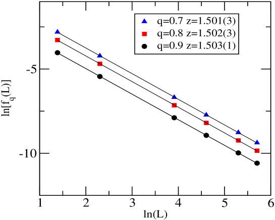
Figure 4: The logarithm of $f_{q}(L)$, given in (30) as a function of $\ln L$ for the stochastic model with parameters $q=0.7,0.8,0.9$ in the in the half-filling sector $n=L$. The dynamical exponent is close the expected value $z=\frac{3}{2}$.

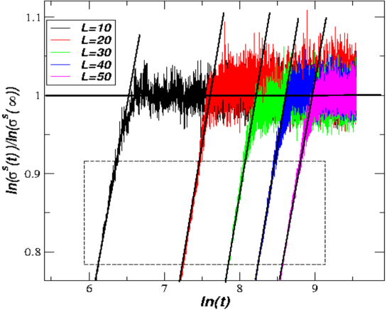
Figure 5: The ratio $\sigma^{s}(t)/\sigma^{s}(\infty)$, as defined in (31), of the standard deviation of the local density of sleeping ants, as a function of time. The results were obtained from Monte Carlo simulations for the cellular automaton in the sector with $n=L$ (half-filled) ants and with parameters $p=1$ and $q=0.75$. At the initial state all the $L$ craters are occupied by a single sleeping ant. The dashed box gives the region used for the linear fit to extract the typical decay time $\tau_{L}$ (see text).The results are the average of $10^{7}$ samples for each lattice size.

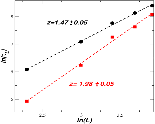
Figure 6: The typical decay time $\tau_{L}$, for lattice sizes $L=20,20,30,40$ and $50$. The dashed box gives the region used for the linear fit to extract the typical decay time $\tau_{L}$ (see text). The squares are obtained from Fig. 5, where $p=1$ and $q=0.75$. The circles are the results obtained for the symmetric case $p=q=1/2$. Both figures were obtained by the same procedure and number of samples. The estimated values for the dynamical critical exponent $z$ are also close to the values $3/2$ and $2$.

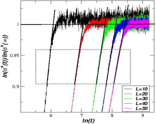
Figure 7: The ratio $\sigma^{s}(t)/\sigma^{s}(\infty)$, as defined in (31), of the standard deviation of the local density of sleeping ants, as a function of time. The results were obtained from Monte Carlo simulations of the cellular automaton with a small local change of the dynamical rules defined in Sec. II (see the text). As in Fig. 5 the parameters are $p=1$ and $q=0.75$ and $10^{7}$ samples were considered for each lattice size. The dashed box delineate the region where a linear fit is done to extract the typical decay time $\tau_{L}$ (see text).

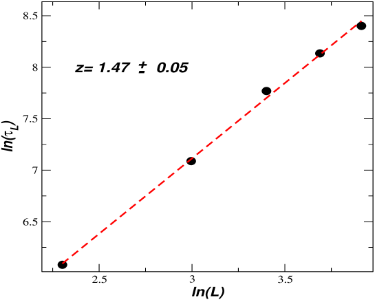
Figure 8: The typical decay time $\tau_{L}$, for lattice sizes $L=20,20,30,40$ and $50$ obtained from Fig. 7. The estimated value for the dynamical critical exponent $z$ is shown in the figure.

V Monte Carlo simulations

In order to check and illustrate the results of last section we present some Monte Carlo simulations (MCS) of the stochastic cellular automaton whose dynamic rules were defined in Sec. II. We consider, as in last section, the case where the number of ants is equal to the lattice size $n=L$ (half-filled lattice).

It is not simple to calculate the dynamical critical exponent $z$ of models in the KPZ universality class by measuring directly the decay-time of observables starting on a given initial condition. A known way is by considering the time-correlations of tagged particles (ants in the present case)tag1 ; tag2 . We verified that, alternatively, this exponent can also be calculated by measuring the time evolution of the variance of a local operator in a given site. In particular by defining $n^{s}(i,t)$ as the occupation number (0 or 1) of a sleeping ant at site $i$ and time $t$, we consider the measure

$$\sigma^{s}(t)=\sqrt{\frac{1}{L}\sum_{i=1}^{L}<[n^{s}(i,t)-<n^{s}>_{\infty}]^{2}>},$$ (31)

where $<n^{s}>_{\infty}$ is the asymptotic average number of sleeping ants in a given site.

We consider two kinds of initial states. Initially we consider a state not translational invariant. We take $L/2$ consecutive craters double occupied (one sleepy and one awake ant) and the remaining craters empty. In Fig. 5 we show the ratio $\sigma^{s}(t)/\sigma^{s}(\infty)$ for lattice sizes $L=10,20,30,40$ and $50$, and parameters $p=1$, $q=0.75$. We estimate from this figure the typical times $\tau_{L}$ where the systems of size $L$ reach the stationary state. These typical times are estimated from the crossing with the value 1 of the straight line obtained from the fitting in the region represented by a dash box in Fig. 5. As we can see the time decay $\tau_{L}$ increases with the lattice size. The dynamical critical exponent $z$ is calculated from the finite-size behavior $\tau_{L}\sim L^{z}$. In Fig. 6 we fit the values of $\ln(\tau_{L})$ with $\ln(L)$ and obtain the estimate $z=1.54\pm 0.05$, in agreement with the expected value $z=3/2$. In the case where the cellular automaton has parameters $p=q=1/2$, i. e. the symmetric case, we expect that the dynamics is pure diffusive. For the sake of comparison we also show in Fig. 6 the lattice dependence of the typical decay time obtained for this symmetric case. We obtain in this case $z=2.02\pm 0.05$, in agreement with a standard diffusive behavior where $z=2$.

We also consider initial states that are translational invariant, as for example the one where we have a single awake ant on each crater ($n=L$). We verified that by using the stochastic rules that define the cellular automaton introduced in section II it is difficult to extract the dynamical critical exponent $z$. In this case the typical times where the system achieve the stationary state is quite small. We can however extract some reliable estimate of $z$ by introducing a small local change in the dynamical rules, that keeps the model on the same universality class of critical behavior. The modified dynamics keeps the number of ants conserved but the last crater ($L$) is special. If we have an awake ant at this crater or there is no ants coming to occupy this crater (coming from crater 1) the rules are the ones that define the cellular automaton (see Fig. 2). However if one ant is coming (from crater 1) and there is no awake ant at crater $L$, there is two possibilities with distinct transition probabilities. If there is no ant at crater $L$ with probability $p$ the arriving ant stays sleeping at the crater $L$, and with probability $1-p$ goes to the crater $L-1$, staying awake. If there is already a sleeping ant with probability one the awake ant that comes from crater 1, goes directly to crater $L-1$ staying awake, and leaving at crater $L$ the sleeping ant. In Fig. 7 we show the ratio $\sigma^{s}(t)/\sigma^{s}(\infty)$ for the same lattice sizes and parameters as in Fig. 5. In Fig. 8 we show the dependence of the typical times $\tau_{L}$ to reach the stationary state as a function of the lattice size $L$. We obtain from this last curve the estimate $z=1.47\pm 0.05$, again in agreement with the KPZ expected value $z=3/2$, as predicted by the exact solution of section IV.

VI Conclusion

In the present work we obtained the exact solution of a probabilistic cellular automaton related to the diagonal-to-diagonal transfer matrix of the asymmetric six-vertex model in a square lattice. The model describes the flow of ants (or particles) on a one-dimensional lattice where we have sleeping or awake ants on a ring of $L$ craters. The solution was obtained by a matrix-product ansatz that can be seen as a matrix product formulation of the coordinate Bethe ansatz. Solving numerically the Bethe ansatz equations we calculated the spectral gap of the model. From the finite-size dependence of the spectral gap we verified that the model belongs to the KPZ universality class displaying a dynamical exponent $z=\frac{3}{2}$. This result was also verified from MCS. The evaluation of this exponent using MCS can be done by measuring the time evolution of the standard deviation of local operators. The lattice-size dependence of the decay time to the stationary state give us an estimator for $z$. Reliable results are obtained by initiating the system in a non translational invariant state. We can also obtain estimates for $z$ starting with translational invariant states ,provide a small local change of the dynamics, playing the rule of a ”defect”, is done.

References

- (1) E. H. Lieb, Residual entropy of square ice, Phys. Rev. 162 (1967).
- (2) Tarasov V O, Takhtajan L A and Fadeev L D, 1983 Theor. Math. Phys. 57 1059
- (3) E. H. Lieb E H, 1967 Phys. Rev. 162 162
- (4) Sutherland B, Yang C N and Yang C P, 1967 Phys. Rev. Lett. 19 588
- (5) Baxter R J, 1982 Exactly solved models in statistical mechanics (Academic Press: London)
- (6) Gaudin M, 1983 La Fonction d’Onde de Bethe (Masson: Paris)
- (7) A. A. Lushnikov, Zh. Éksp. Teor. Fiz. 91, 1376 (1986) [Sov. Phys. JETP 64, 811 (1986)], Phys. Lett. A 120, 135 (1987).
- (8) G. M. Schütz, J. Stat. Phys. 71, 471 (1993).
- (9) F. C. Alcaraz, M. Droz, M. Henkel, and V. Rittenberg, Ann. Phys. (N.Y.) 230, 250 (1994).
- (10) F. C. Alcaraz and V. Rittenberg, Phys. Lett. B 324, 377 (1993).
- (11) F. C. Alcaraz, Int. J. Mod. Phys. B bf 8, 3449 (1994).
- (12) M. D. Grynberg and R. B. Stinchcombe, Phys. Rev. Lett. 74, 1242 (1995).
- (13) K. Krebs, M. P. Pfannmüller, B. Wehefritz, and H. Henrichsen, J. Stat. Phys. 78, 1429 (1995).
- (14) J. E. Santos, G. M. Schütz, and R. B. Stinchcombe, J. Chem. Phys. 105, 2399 (1996).
- (15) M. J. de Oliveira, T. Tomé, and R. Dickman, Phys. Rev. A 46, 6294 (1992).
- (16) L. H. Gwa and H. Spohn, Phys. Rev. Lett. 68, 725 (1992), Phys. Rev. A 46, 844 (1992).
- (17) D. J. Bukman and J. D. Shore, J. Stat. Phys. 78, 1277 (1995); I. M. Nolden, J. Stat. Phys. 67, 155 (1992).
- (18) A. Borodin, I. Corwin and V. Gorin, arXiv:1407.6729.
- (19) T. Halpin-Healy and K. A. Takeuchi, arXiv:1505.01910
- (20) D. Kim, Phys. Rev. E 52, 3512 (1995), J. Phys. A 30, 3817 (1997).
- (21) F. C. Alcaraz, S. Dasmahapatra and V. Rittenberg, J. Phys. A. 31, 845 (1998).
- (22) T. Sasamoto and M. Wadati, J. Phys. A 31, 6057 (1998).
- (23) F. C. Alcaraz and R. Z. Bariev, Phys. Rev. E 60, 79 (1999).
- (24) B. Derrida, Physics Reports 301, 65 (1998).
- (25) T. M. Ligget, Stochastic Interacting Systems: Contact, Voter and Exclusion Process (Springer Verlag, 1999).
- (26) F. C. Alcaraz and R. Z. Bariev, Braz. J. Phys. 30, 13 (2000).
- (27) F. C. Alcaraz and R. Z. Bariev, Braz. J. Phys. 30, 655 (2000).
- (28) G. M. Schütz, Integrable Stochastic Many-body Systems in ”Phase Transition and Critical Phenomena”, vol. 19, Eds. C. Domb and J. L. Lebowitz (Academic, London, 2000).
- (29) V. E. Korepin, A. G .Izergin and N. M. Bogoliubov, Quantum Inverse Scattering Method, Correlation Functions and Algebraic Bethe Ansatz (Cambridge University Press, Cambridge, 1992).
- (30) F. H. L. Essler and V. E. Korepin, Exactly Solvable Models of Strongly Correlated Electrons (World Scientific, Singapore, 1994).
- (31) P. Schlottmann, Int. J. Mod. Physics B, 11, 355 (1997).
- (32) D. Kandel, E. Domany and B. Nienhuis, J. Phys. A: Math. Gen. 23, L755 (1990).
- (33) F. C. Alcaraz and R. Z. Bariev, Physica A 306 51 (2002).
- (34) R. Z. Bariev, Mat. Fiz. 49 (1981)
- (35) M. Kardar, G. Parisi and Y. C. Zhang, Phys. Rev. Lett. 56, 889 (1986).
- (36) K. Nishinari, K. Sugawara, T. Kazama, A. Schdschneider and D. Chowdhury, arXiv:0702584.
- (37) H.A. Bethe, Z. Phys. 71 205 (1931).
- (38) F. C. Alcaraz and M. J. Lazo, J. Phys. A: Math. Gen. 37 L1 (2004).
- (39) F. C. Alcaraz and M. J. Lazo, J. Phys. A: Math. Gen. 37 4149 (2004).
- (40) F. C. Alcaraz and M. J. Lazo, J. Phys. A: Math. Gen. 39 11335 (2006).
- (41) F. C. Alcaraz and M. J. Lazo, Braz. J. Phys. 33 533 (2003).
- (42) M. J. Lazo and A. A. Ferreira, Phys. Rev. E 81 050104 (2010).
- (43) M. J. Lazo and A. A. Ferreira, J. Stat. Mech. P05017 (2012).
- (44) A. A. Ferreira and F. C. Alcaraz, Phys. Rev. E 74 011115 (2006).
- (45) M. J. Lazo, Physica A 374 655 (2007).
- (46) F. C. Alcaraz and M. J. Lazo, J. Stat. Mech. P08008 (2007).
- (47) F. C. Alcaraz, M. N. Barber, and M. T. Batchelor, Phys. Rev. Lett. 58 771 (1987); Ann. Phys. 182, 280 (1988).
- (48) M. T. Batchelor, M. N. Barber, and P. A. Pearce, J. Stat. Phys. 49 1117 (1987).
- (49) S. N. Majumdar and M. Barma, Phys. Rev. B 44 5306 (1991).
- (50) A. A. Ferreira and F. C. Alcaraz, Phys. Rev. E 65 052102 (2002).