Fourth-order QCD renormalization group quantities in the V-scheme and the relation of the $\beta$-function to the Gell-Mann–Low function in QED

Abstract

The semi-analytical $O(\alpha_{s}^{4})$ expression for the renormalization group $\beta$ function in the ${\rm{V}}$ scheme is obtained in the case of the $SU(N_{c})$ gauge group. In the process of calculations we use the existing information about the three-loop perturbative approximation for the QCD static potential, evaluated in the $\rm{\overline{MS}}$ scheme. The comparison of the numerical values of the third and fourth coefficients for the QCD RG $\beta$ functions in the gauge-independent ${\rm{V}}$ and $\rm{\overline{MS}}$ schemes and in minimal momentum scheme in the the Landau gauge is presented. The phenomenologically oriented comparisons for the coefficients of $O(\alpha_{s}^{4})$ expression for the $e^{+}e^{-}$-annihilation R-ratio in these schemes are presented. It is shown that taking into account these QCD contributions is of vital importance and lead to a drastic decrease of the scheme-dependence ambiguities of the fourth-order perturbative QCD approximations for the $e^{+}e^{-}$ annihilation R-ratio for the number of active flavours, $n_{f}=5$ in particular. We demonstrate that in the case of QED with $N$-types of leptons the coefficients of the $\beta^{\rm{V}}$ function are closely related to the ones of the Gell-Mann–Low $\Psi$ function and emphasise that they start to differ from each other at the fourth order due to the appearance of the extra $N^{2}$-contribution in the V scheme. The source of this extra correction is clarified. The general all-order QED relations between the coefficients of the $\beta^{\rm{V}}$ and $\Psi$ functions are discussed.

I Introduction

The renormalization group (RG) $\beta$ function is one of the basic quantities of the RG method, which was developed in the classical works of Refs.Stueckelberg:1953dz , Bogolyubov:1956gh , GellMann:1954fq . It defines the energy behaviour of the renormalized coupling constants of the renormalized quantum field models. It is known that in the case when the quantum field model under study has the single coupling constant, the perturbation theory (PT) expressions for its RG $\beta$-functions depend on the choice of the scheme of subtracting ultraviolet (UV) divergences.

In QED the first and the second coefficients of the $\beta$ function are scheme independent and were obtained in Ref. GellMann:1954fq from the analytical calculations of the two-loop approximation for the renormalized photon propagator performed in Ref. JL .

In the momentum (MOM) scheme, defined by subtractions of the UV divergences of the photon vacuum polarization function at the non-zero Euclidean point $\lambda^{2}$, the QED RG $\beta$ function coincides with the Gell-Man–Low function $\Psi(\alpha_{\rm{MOM}})$, where the expression for $\alpha_{\rm{MOM}}(q^{2})$ coincides with the QED invariant charge, uniquely defined by the combinations of the Green functions Bogolyubov:1980nc . The expressions for the coefficients of the PT series for $\Psi(\alpha_{\rm{MOM}})$ depend on the number of leptons $N$.

For $N$=1, i.e. in the case of consideration of the electron only, the three-loop term of the $\Psi$ function was calculated analytically in Ref. Baker:1969an . This result was generalized to the case of the arbitrary number $N$ of massless leptons in Ref. Gorishnii:1987fy . The $N$-dependent expressions for the four- and five-loop corrections to the Gell-Man–Low function were evaluated symbolically in Refs. Gorishnii:1990kd and Baikov:2012zm respectively. At $N$=1 the result of Ref. Baikov:2012zm coincides with the similar expression, obtained in Ref. Kataev:2012rf . This feature should be considered as the strong argument in favour of the consistency of the complicated analytical five-loop calculations, performed in Ref. Baikov:2012zm .

Another important scheme, which is used in QED, is the on-shell (OS) scheme. In this scheme the photon vacuum polarization function is defined by subtracting UV divergences at zero transferred momentum, while the renormalized on-shell masses of leptons are identified with their experimentally measured values.

In the physical OS scheme the calculations of the $\beta(\alpha_{\rm{OS}})$ were performed at the three-loop level in the work of DeRafael:1974iv . The analytical expression for the corresponding four-loop correction was obtained in Ref. Broadhurst:1992za . In the case of arbitrary $N$ the five-loop contribution was obtained in Ref. Baikov:2012rr . It is in agreement with the result of the work Kataev:2012rf , where this term was obtained at $N$=$1$ with the help of the concrete RG-relations. The agreement with the outcome of the direct five-loop calculations of Ref. Baikov:2012rr gives extra confidence in the correctness and self-consistency of the results of the complicated computer calculations used in Ref. Kataev:2012rf .

The third class of schemes, which we are interested in, is introduced when the dimensional regularization 'tHooft:1972fi is used. These schemes include the minimal subtractions (MS) scheme 'tHooft:1973mm and its modified variants, namely the $\rm{\overline{MS}}$-scheme Bardeen:1978yd and the G scheme Chetyrkin:1980pr . It is possible to prove that for all these modifications of the MS scheme the coefficients for the RG $\beta$ functions coincide in all orders of PT.

At $N$=1 the three-loop correction to the $\beta(\alpha_{\rm{\overline{MS}}})$ function was evaluated in Refs. Chetyrkin:1980pr and Vladimirov:1979zm independently (this result had been also presented in the review of Ref. Vladimirov:1979ib ). In the case of the arbitrary $N$ the three-loop contribution to $\beta(\alpha_{\overline{\rm{MS}}})$ was obtained analytically in Ref. Gorishnii:1987fy . The computation of the four-loop term was completed in Ref. Gorishnii:1990kd . The five-loop correction to the QED $\beta$ function in the MS-like schemes was calculated in Ref. Baikov:2012zm . At $N$=1 this expression coincides with the result of non-direct analysis, performed in Ref. Kataev:2012rf .

It is known that in QCD the MS-like schemes maintain the explicit gauge independence of various RG quantities. This property clarifies why in multiloop QCD calculations the MS-like schemes are used more often. In QCD the first coefficient of the $\beta$-function was computed in Refs. Gross:1973id ,Politzer:1973fx and for the number of quarks flavours $n_{f}\leq 6$ turned out to be negative. This feature revealed the existence of the asymptotic-freedom property in the gauge theory of strong interactions. The two-loop correction to the QCD $\beta$ function in the MS-like scheme was analytically evaluated in Jones:1974mm , Caswell:1974gg , Egorian:1978zx and is also negative .

At the three-loop level the QCD $\beta$ function was analytically calculated in the $\rm{\overline{MS}}$ scheme in Ref. Tarasov:1980au . This result was confirmed later in Ref. Larin:1993tp . The four-loop term of the QCD $\beta$ function in the MS-like schemes was evaluated in Ref. vanRitbergen:1997va and confirmed in Ref. Czakon:2004bu . For $n_{f}$=$6$ the three-loop correction to the $\beta$ function in the MS-like schemes is positive (see the numerical results presented below). Note however that the resummation of the PT series for the QCD $\beta$ function in the MS-like schemes gives the arguments that this feature does not affect the asymptotic freedom property Kazakov:2003df .

In QCD one can also use another gauge-independent scheme, namely the V scheme. It was first introduced in Refs. Peter:1996ig , Schroder:1998vy and is determined by perturbative high order QCD corrections to the static potential. This scheme was used in Ref. Brodsky:1999fr to model massive dependence of the first two coefficients of the RG $\beta$ function in the V scheme and for the related analysis of the manifestation of the massive-dependent corrections in the effect of running of the QCD coupling constant from the energies above the production of charm quarks to the high energy region above the scale $s$=$M_{Z}^{2}$. In this case the advantage of using the V scheme and not the ${\rm{\overline{MS}}}$ scheme is contained in the possibility of modelling the smooth transition of the QCD coupling constant through the thresholds of heavy quarks productions. Among other applications of the V scheme in QCD is the analysis of the perturbative QCD predictions for $\Gamma(H^{0}\rightarrow b\overline{b})$ Broadhurst:2000yc . It was shown in this work that within the large $\beta_{0}$-expansion the perturbative approximations for $\Gamma(H^{0}\rightarrow b\overline{b})$ in the ${\rm{V}}$ scheme are converging to the concrete stable value faster than in the ${\rm{\overline{MS}}}$ scheme.

However, to analyse more carefully the behaviour of various perturbative QCD series for the observable physical quantities in the V scheme it is necessary to know high-order PT corrections to the QCD $\beta$ function in this scheme. In the present work we will get the semi-analytical result for the fourth coefficient of the QCD $\beta$ function in the ${\rm{V}}$ scheme, i.e. for the $\beta^{\rm{V}}$ function. In Sec. II the available results of the analytical and semi-analytical calculations of the PT QCD corrections to the static potential $\rm{V_{QCD}}(\alpha_{s}(\mu^{2}))$ in the ${\rm{\overline{MS}}}$ scheme are summarized. The concrete three-loop results, obtained by two groups of authors, are compared. Section III is devoted to the definition of the ${\rm{V}}$ scheme and to the presentation of the concrete results for the third and fourth coefficients of the $\beta^{\rm{V}}$ function. The problem of finding the analytical expression for the concrete known numerical contributions to the fourth-order term of the $\beta^{\rm{V}}$ function is raised. In Sec. IV the numerical values for the scheme-dependent coefficients of the QCD $\beta$ function in the V scheme are compared with the similar terms, obtained in the MS-like schemes and in the gauge-dependent minimal-MOM (mMOM) scheme widely used at present, defined in Ref. vonSmekal:2009ae . We also get the $O(\alpha_{s}^{4})$ expression for the $e^{+}e^{-}$-annihilation R-ratio in the V scheme and compare it with gauge-independent scheme and gauge-dependent mMOM scheme results. In fact both $\rm{\overline{MS}}$ and mMOM scheme were applied recently for the analysis of the behaviour of R-ratio in the fourth order of PT Ref. Gracey:2014pba . Using the concrete physical input, we modify this analysis and emphasize that it is more consistent to perform this comparison for $n_{f}=4,5$ numbers of active flavours in the energy-region above the production of charm-quark pairs and below $s\approx 900~{}\rm{GeV^{2}}$, where the effects of subprocess $e^{+}e^{-}\rightarrow Z^{0}\rightarrow{\rm{hadrons}}$ did not yet start to manifest itself. In Sec. V we consider the QED limit of the results obtained in Sec. III and obtain the expression for the $O(\alpha_{\rm{V}}^{5})$ approximation of the $\beta^{\rm{V}}$ function in QED. The origin of difference with the QED Gell-Man–Low $\Psi$ function, which is starting to manifest itself from the fourth term, is demonstrated and explained. The existing common features of the PT series for the $\Psi$ and $\beta^{\rm{V}}$ functions is clarified in all orders of PT.

II Preliminaries: the high-order expression of the static potential in QCD in the $\rm{\overline{MS}}$ scheme

Let us first summarise the available information about the perturbative QCD contributions to the static potential known at present. This physical quantity is used in various phenomenologically oriented QCD studies, e.g. in the process of theoretical determinations of the charm, bottom and top quark masses, and for the studies of the properties of different mesons, composed from the $c$ and $b$ quarks (see e.g. Pineda:1998ja ,Ayala:2014yxa ,Kiyo:2014uca and references therein).

Within PT the static potential in QCD is defined as a renormalized expression for the potential of interaction at a distance r between static heavy quark $Q_{h}$ and anti-quark $\overline{Q}_{h}$. It is expressed through the following Fourier representation

$$\rm{V}_{QCD}(\mu^{2}r^{2},\alpha_{s}(\mu^{2})) = \int\frac{d^{3}\vec{q}}{(2\pi)^{3}}e^{i\vec{q}\vec{r}}{\rm{V}}(\vec{q^{2}},\mu^{2},\alpha_{s}(\mu^{2}))$$

$$= \int\frac{d^{3}\vec{q}}{(2\pi)^{3}}e^{i\vec{q}\vec{r}}\bigg{(}-4\pi C_{F}\frac{\alpha_{s,V}(\vec{q^{2}}/\mu_{V}^{2})}{\vec{q^{2}}}\bigg{)}$$

where $\alpha_{s,V}(\vec{q^{2}}/\mu_{V}^{2})$ is the renormalized QCD coupling constant in V scheme, $\alpha_{s}/4\pi=g^{2}/16\pi^{2}$, $g$ is the strong coupling constant of the QCD Lagrangian, $T^{a}$ is the generator of the $SU(N_{c})$ group, normalized as $T^{a}=\lambda^{a}/2$ and $C_{F}$ is the Casimir operator, defined as $(T^{a}T^{a})_{ij}=C_{F}\delta_{ij}$. In the V scheme its coupling constant $\alpha_{s,V}(\vec{q^{2}}/\mu_{V}^{2})$ is related to the numerator of the momentum representation of the static potential in the $\overline{\rm{MS}}$ scheme defined in Eq. (II) and is expressed as

$$\alpha_{s,V}(\vec{q^{2}}/\mu_{V}^{2})=\alpha_{s}(\mu^{2})P(\alpha_{s}(\mu^{2}),L)=\alpha_{s}(\mu^{2})\sum_{n=0}^{\infty}P^{\rm{\overline{MS}}}_{n}(L)\bigg{(}\frac{\alpha_{s}(\mu^{2})}{4\pi}\bigg{)}^{n}~{}~{}~{}.$$ (2)

The rhs of Eq. (2) is expressed through higher-order PT QCD corrections to the static potential $P^{\rm{\overline{MS}}}_{n}(L)$ in the $\rm{\overline{MS}}$ scheme which are known at present up to $O(\alpha_{s}^{3})$-level and will be presented below.

The evolution of the $\rm{\overline{MS}}$ scheme coupling constant $\alpha_{s}(\mu^{2})$ (which depends on the $\rm{\overline{MS}}$ scheme renormalization parameter $\mu^{2}$) is governed by the QCD $\rm{\overline{MS}}$ scheme $\beta$ function:

$$\mu^{2}\frac{\partial(\alpha_{s}/4\pi)}{\partial\mu^{2}}=\beta^{\rm{\overline{MS}}}(a_{s})=-\sum_{i=0}^{\infty}\beta_{i}\bigg{(}\frac{\alpha_{s}}{4\pi}\bigg{)}^{i+2}~{}~{},$$ (3)

where $a_{s}=\alpha_{s}/4\pi$ and its known four $\rm{\overline{MS}}$ scheme coefficients, taken from the work of Ref. vanRitbergen:1997va , read:

$$\beta_{0} = \frac{11}{3}C_{A}-\frac{4}{3}T_{F}n_{l}$$ (4)

$$\beta_{1} = \frac{34}{3}C^{2}_{A}-4C_{F}T_{F}n_{l}-\frac{20}{3}C_{A}T_{F}n_{l}$$ (5)

$$\beta_{2} = \frac{2857}{54}C^{3}_{A}+2C^{2}_{F}T_{F}n_{l}-\frac{205}{9}C_{F}C_{A}T_{F}n_{l}-\frac{1415}{27}C^{2}_{A}T_{F}n_{l}+$$

$$+ \frac{44}{9}C_{F}T^{2}_{F}n^{2}_{l}+\frac{158}{27}C_{A}T^{2}_{F}n^{2}_{l}$$

$$\beta_{3} = \left(\frac{150653}{486}-\frac{44}{9}\zeta(3)\right)C^{4}_{A}+\left(-\frac{39143}{81}+\frac{136}{3}\zeta(3)\right)C^{3}_{A}T_{F}n_{l}$$

$$+ \left(\frac{7073}{243}-\frac{656}{9}\zeta(3)\right)C^{2}_{A}C_{F}T_{F}n_{l}+\left(-\frac{4204}{27}+\frac{352}{9}\zeta(3)\right)C_{A}C^{2}_{F}T_{F}n_{l}$$

$$+ 46C^{3}_{F}T_{F}n_{l}+\left(\frac{7930}{81}+\frac{224}{9}\zeta(3)\right)C^{2}_{A}T^{2}_{F}n^{2}_{l}$$

$$+ \left(\frac{1352}{27}-\frac{704}{9}\zeta(3)\right)C^{2}_{F}T^{2}_{F}n^{2}_{l}+\left(\frac{17152}{243}+\frac{448}{9}\zeta(3)\right)C_{A}C_{F}T^{2}_{F}n^{2}_{l}$$

$$+ \frac{424}{243}C_{A}T^{3}_{F}n^{3}_{l}+\frac{1232}{243}C_{F}T^{3}_{F}n^{3}_{l}+\left(-\frac{80}{9}+\frac{704}{3}\zeta(3)\right)\frac{d^{abcd}_{A}d^{abcd}_{A}}{N_{A}}$$

$$+ \left(\frac{512}{9}-\frac{1664}{3}\zeta(3)\right)\frac{d^{abcd}_{F}d^{abcd}_{A}}{N_{A}}n_{l}+\left(-\frac{704}{9}+\frac{512}{3}\zeta(3)\right)\frac{d^{abcd}_{F}d^{abcd}_{F}}{N_{A}}n^{2}_{l}$$

The characteristic colour structures of the group $SU(N_{c})$ are defined as in the detailed work of Ref. vanRitbergen:1998pn . In the notations of Ref. vanRitbergen:1998pn we have $[T^{a},T^{b}]=if^{abc}T^{c}$, where $f^{abc}$ are the antisymmetric (under permutations of any pair of indices) structure constants, which satisfy the well-known relation $f^{acd}f^{bcd}=C_{A}\delta^{ab}$, $C_{A}$ and $C_{F}$ are the Casimir operators, $Tr(T^{a}T^{b})=T_{F}\delta^{ab}$, $N_{A}$ is the number of the generators of the Lie algebra of the $SU(N_{c})$, $n_{l}$ is the number of quarks flavors, $d^{abcd}_{F}=Tr(T^{a}T^{(b}T^{c}T^{d)})/6\;$ is the totally symmetric tensor. The notations ^(…) are defining the procedure of symmetrisation of the generators $T^{b}T^{c}T^{d}$, $d^{abcd}_{A}=Tr(C^{a}C^{(b}C^{c}C^{d)})/6\;$ is the total symmetric tensor of $(C^{a})_{bc}=-if^{abc}$, where $C^{a}$ are the generators of the adjoint representation of the Lie algebra of the $SU(N_{c})$-group. The corresponding colour structures in Eqs.(4)-(II) have the following form vanRitbergen:1997va :

$$C_{A}=N_{c}~{}~{}~{}~{}~{},~{}~{}~{}~{}~{}C_{F}=\frac{N_{c}^{2}-1}{2N_{c}}~{}~{}~{}~{}~{},~{}~{}~{}~{}N_{A}=N_{c}^{2}-1$$ (8)

$$\frac{d_{A}^{abcd}d_{A}^{abcd}}{N_{A}}=\frac{N_{c}^{2}(N_{c}^{2}+36)}{24}~{},~{}\frac{d_{F}^{abcd}d_{A}^{abcd}}{N_{A}}=\frac{N_{c}(N_{c}^{2}+6)}{48}~{}~{}$$ (9)

$$\frac{d_{F}^{abcd}d_{F}^{abcd}}{N_{A}}=\frac{N_{c}^{4}-6N_{c}^{2}+18}{96N_{c}^{2}}~{}~{}~{}~{}.$$ (10)

The terms, proportional to the n-th powers of $L=\ln\left(\mu^{2}/\vec{q^{2}}\right)$, $P^{\rm{\overline{MS}}}_{n}(L)$ in the polynomial $P(\alpha_{s}(\mu^{2}))$ of Eq.(2) are expressed as $P^{\rm{\overline{MS}}}_{0}=1$, $P^{\rm{\overline{MS}}}_{1}(L)=a_{1}^{\rm{\overline{MS}}}+\beta_{0}L$, $P_{2}^{\rm{\overline{MS}}}(L)=a_{2}^{\rm{\overline{MS}}}+(2a_{1}^{\rm{\overline{MS}}}\beta_{0}+\beta_{1})L+\beta^{2}_{0}L^{2}$, $P_{3}^{\rm{\overline{MS}}}(L)=a_{3}^{\rm{\overline{MS}}}+(3a_{2}^{\rm{\overline{MS}}}\beta_{0}+2a_{1}^{\rm{\overline{MS}}}\beta_{1}+\beta^{\rm{\overline{MS}}}_{2})L+(3a_{1}^{\rm{\overline{MS}}}\beta^{2}_{0}+\frac{5}{2}\beta_{0}\beta_{1}){L}^{2}+\beta^{3}_{0}{L}^{3}$. The powers of $L$ in the expressions presented above arise from the solutions of the corresponding RG equations in the MS-like schemes at the three-loop level.

The coefficients $a_{i}^{\rm{\overline{MS}}}$ are calculated from the concrete Feynman diagrams. The first one, $a_{1}^{\rm{\overline{MS}}}$, was calculated long time ago in Refs. Fischler:1977yf , Billoire:1979ih and has the following form

$$a_{1}^{\rm{\overline{MS}}}=\frac{31}{9}C_{A}-\frac{20}{9}T_{F}n_{l}$$ (11)

where $n_{l}=n_{f}-1$. The coefficient $a_{2}^{\rm{\overline{MS}}}$ was obtained in the Peter:1996ig . The bug in the pure Yang-Mills contribution to $a_{2}^{\rm{\overline{MS}}}$, evaluated in Refs. Peter:1996ig , was detected in Ref. Schroder:1998vy .

The final result of these analytical calculations of Refs. Peter:1996ig , Schroder:1998vy is

$$a_{2}^{\rm{\overline{MS}}} = \bigg{(}\frac{4343}{162}+4\pi^{2}-\frac{\pi^{4}}{4}+\frac{22}{3}\zeta(3)\bigg{)}C^{2}_{A}-\left(\frac{1798}{81}+\frac{56}{3}\zeta(3)\right)C_{A}T_{F}n_{l}$$ (12)

$$- \left(\frac{55}{3}-16\zeta(3)\right)C_{F}T_{F}n_{l}+\left(\frac{20}{9}T_{F}n_{l}\right)^{2}~{}~{}~{}~{}.$$

The three-loop constant perturbative contribution to the static potential in the $\rm{\overline{MS}}$ scheme can be presented as

$$a_{3}^{\rm{\overline{MS}}}=a^{(3)}_{3}n^{3}_{l}+a^{(2)}_{3}n^{2}_{l}+a^{(1)}_{3}n_{l}+a^{(0)}_{3}~{}~{}~{}.$$ (13)

The $n_{l}$-dependent terms were computed in Ref. Smirnov:2008pn and have the following form:

$$a^{(3)}_{3} = -\bigg{(}\frac{20}{9}\bigg{)}^{3}T^{3}_{F}$$ (14)

$$a^{(2)}_{3} = \left(\frac{12541}{243}+\frac{368}{3}\zeta(3)+\frac{64\pi^{4}}{135}\right)C_{A}T^{2}_{F}+\left(\frac{14002}{81}-\frac{416}{3}\zeta(3)\right)C_{F}T^{2}_{F}$$ (15)

$$a^{(1)}_{3} = -709.717C^{2}_{A}T_{F}+\left(-\frac{71281}{162}+264\zeta(3)+80\zeta(5)\right)C_{A}C_{F}T_{F}$$

$$+ \left(\frac{286}{9}+\frac{296}{3}\zeta(3)-160\zeta(5)\right)C^{2}_{F}T_{F}-56.83(1)\frac{d^{abcd}_{F}d^{abcd}_{F}}{N_{A}}$$

where the error of numerical calculation of the $C_{A}^{2}T_{F}$-coefficient in Eq. (II) is not indicated in Ref. Smirnov:2008pn .

It is worth emphasizing that in the QED limit with $C_{A}$=$0$, the analytical expressions of the $n_{l}$-dependent terms, which are proportional to the powers of $T_{F}$ in Eqs. (11),(12) and in Eqs. (14)-(II), are in agreement with the $\rm{\overline{MS}}$-scheme results presented in Gorishnii:1991hw for the constant terms of the three-loop approximation of the photon vacuum polarization function in QED. They were also confirmed in Ref. Baikov:2012rr in the process of computation of the four-loop approximation of this quantity. The agreement with the QED results of Refs. Gorishnii:1991hw gives us extra confidence in the validity of the outcomes of calculations of Ref. Smirnov:2008pn .

The numerical expressions of the $n_{l}$-independent contributions to Eq. (13) were obtained in Ref. Smirnov:2009fh and read

$$a^{(0)}_{3}=502.24(1)C^{3}_{A}-136.39(12)\frac{d^{abcd}_{F}d^{abcd}_{A}}{N_{A}}$$ (17)

These results should be compared with the results of the independent calculation of Ref. Anzai:2009tm

$$a^{(0)}_{3}=502.22(12)C^{3}_{A}-136.8(14)\frac{d^{abcd}_{F}d^{abcd}_{A}}{N_{A}}$$ (18)

which have greater inaccuracies. Recently the more accurate result for the second term in Eq. (18) was obtained with the help of the computer code used in Ref. Anzai:2009tm . The improved result for Eq. (18) is:

$$a^{(0)}_{3}=502.22(12)C^{3}_{A}-136.6(2)\frac{d^{abcd}_{F}d^{abcd}_{A}}{N_{A}}$$ (19)

The numerical expression of the coefficient before the second structure in Eq. (19) is in agreement with the numerical expression of the same coefficient in Eq. (17) and demonstrates the reliability of the computer codes, created in the process of calculations, which were performed in Ref. Smirnov:2009fh and Ref. Anzai:2009tm .

The three-loop $n_{l}$-independent correction to the static potential also contains the RG non-controllable additional term $8\pi^{2}C_{A}^{3}L$ Kniehl:2002br . It is associated with the infrared (IR) divergences, which begin to manifest themselves in the the static potential at the three-loop level Appelquist:1977es , Brambilla:1999qa . In the effective theory of heavy quarkonium – nonrelativistic QCD– these IR-divergent $L$-terms are cancelled by the concrete UV-divergent contributions (see e.g. Brambilla:1999qa ).

Among the aims of this work is the determination of the four-loop approximation of the RG $\beta$ function in the V scheme. This can be done by application of the RG-motivated effective charges (ECH) approach, developed in all orders of PT in the works of Refs. Grunberg:1980ja ,Grunberg:1982fw and independently at the next-to-leading order (NLO) in Ref. Krasnikov:1981rp (for the concrete NLO applications see e.g. the work Kataev:1981gr ) The fourth-order approximation of the $\beta$ function in the V scheme defines the evolution of $\alpha_{s,V}$ in the region of intermediate and UV values of energy scales. It does not depend on the manifestation of IR physical effects and on the RG-uncontrollable $L$-dependent corrections to the static potential. In view of this we will not consider them in our further analysis.

III The fourth order approximation of the QCD $\beta$ function in the V scheme

III.1 The scale-scheme dependence ambiguities.

Let us start this section from writing the RG equation for the static potential, which is defined in Eq. (II). In the massless limit, considered in this work, it has the following form

$$\bigg{(}\mu^{2}\frac{\partial}{\partial\mu^{2}}+\beta(a_{s})\frac{\partial}{\partial a_{s}}\bigg{)}{\rm{V}}(\vec{q^{2}},\mu^{2},a_{s}(\mu^{2}))=0$$

In QCD the scheme-dependence feature of the PT series for the RG $\beta$ function is the more delicate issue than the scheme-dependence problem of the QED RG $\beta$ function discussed in the Introduction. Indeed, contrary to the QED case, in this realistic theory of strong interactions it is impossible to introduce straightforwardly the gauge-invariant analog of the MOM scheme (see e.g. Celmaster:1979km , Braaten:1981dv ,Dhar:1981jm ) and thus to construct the invariant charge in a unique gauge-invariant manner. In QCD the number of the invariant-type charges of the MOM schemes is proportional to 4, namely to the number of vertexes of the Lagrangian (i.e. of the gluon-quark-antiquark, gluon-ghost-ghost, three-gluon and the four-gluon vertexes). Moreover, the definitions of these invariant-type charges depend on different kinematic conditions for fixing the scales of subtractions of UV divergences in the renormalized Green functions, which enter these different QCD invariant-type charges. Indeed, fixing the kinematics conditions by a different way it is possible to construct a number of MOM schemes, i.e. the symmetric MOM scheme Celmaster:1979km , the variant of symmetric MOM scheme with one external zero momentum Braaten:1981dv and the asymmetric MOM (AMOM) scheme Dhar:1981jm . Different gauge-dependent MOM schemes were used in the direct calculations of the massless two-loop vonSmekal:2009ae , Raczka:1988my -Gracey:2011pf , three-loop vonSmekal:2009ae , Chetyrkin:2000dq -Gracey:2011pf and even four-loop vonSmekal:2009ae , Chetyrkin:2000fd , Gracey:2013sca corrections to the QCD $\beta$ function. These analytical calculations revealed the importance of the careful study of the dependence on gauge parameter. The classical example of the validity of this statement is the discovery that in the AMOM the non-proper choice of the gauge in the two-loop PT correction to the QCD $\beta$ function can destroy the asymptotic freedom property of the perturbative QCD Raczka:1988my ,Tarasov:1990ps .

Summarizing the discussions of the gauge ambiguities in the QCD analogs of the invariant charges of various MOM schemes, we stress that in these schemes it is impossible to construct gauge-invariant analog of the Gell-Man–Low function. In view of this it is important to study the expansions of the $\beta$ function in terms of physical coupling constants, which enter the effective LO approximations of the RG-invariant physical quantities, e.g. the effective coupling constant of the ${\rm V}$ scheme defined by the QCD static potential Brodsky:1999fr .

In all these studies the ECH method, developed in Refs. Grunberg:1980ja -Krasnikov:1981rp , was used. To remind the basis of this approach consider first the system of Eq. (II) and (2), which defines the expansion of the QCD coupling constant of the ${\rm{V}}$ scheme through the QCD coupling constant in the $\rm{\overline{MS}}$ scheme.

At the first step, following the NLO definition of the ECH scheme, we define the effective scale of the ${\rm{V}}$ scheme as

$$\mu_{V}^{2}=\displaystyle\rm{exp}[a_{1}^{\rm{\overline{MS}}}/\beta_{0}]\mu^{2}_{\rm{\overline{MS}}}$$ (20)

where $a_{1}^{\rm{\overline{MS}}}=\frac{31}{9}C_{A}-\frac{20}{9}T_{F}n_{l}$ and $\beta_{0}$ is the first coefficient of the QCD $\beta$ function, defined in Eq. (3). At the next step we fix $\vec{q^{2}}=\mu_{V}^{2}$ in Eq. (2) and get the following relation between the effective charge of the ${\rm{V}}$ scheme and the QCD coupling constant $\alpha_{s,\overline{\rm{MS}}}$:

$$\alpha_{s,V}(\mu_{V}^{2}) = \alpha_{s,\overline{\rm{MS}}}(\mu_{V}^{2})P(\alpha_{s,\overline{\rm{MS}}},L=0)$$

$$= \alpha_{s,\overline{\rm{MS}}}(\mu_{V}^{2})\bigg{[}1+a_{2}^{\rm{\overline{MS}}}\bigg{(}\frac{\alpha_{s,\overline{\rm{MS}}}(\mu_{V}^{2})}{4\pi}\bigg{)}^{2}+a_{3}^{\rm{\overline{MS}}}\bigg{(}\frac{\alpha_{s,\overline{\rm{MS}}}(\mu_{V}^{2})}{4\pi}\bigg{)}^{3}+O(\alpha_{s,\overline{\rm{MS}}}^{4})\bigg{]}~{}~{}.$$

Now it is possible to define the ECH $\beta$ function of the static potential, which is the RG $\beta$ function in the ${\rm{V}}$ scheme

$$\mu_{V}^{2}\frac{\partial(\alpha_{s,V}/4\pi)}{\partial\mu_{V}^{2}}=\beta^{\rm{V}}(a_{s,V})=-\sum_{i=0}^{\infty}\beta_{i}^{V}\bigg{(}\frac{\alpha_{s,V}}{4\pi}\bigg{)}^{i+2}~{}~{}~{}$$ (22)

where $a_{s,V}=\alpha_{s,V}/4\pi$. The standard RG equation relates $\beta^{\rm{V}}$ function to the $\beta$ function in the MS-like schemes:

$$\beta^{\rm{V}}(a_{s,V}(a_{s,\overline{\rm{MS}}}(\mu_{\rm{V}}^{2}))=\beta^{\rm{\overline{MS}}}(a_{s,\overline{\rm{MS}}}(\mu_{\rm{V}}^{2}))\frac{da_{s,V}(a_{s,\overline{\rm{MS}}}(\mu^{2}_{\rm{V}}))}{da_{s,\overline{\rm{MS}}}(\mu_{\rm{V}}^{2})}~{}~{}~{}.$$ (23)

Consider now the relation between $\beta$ functions, computed in the gauge-invariant UV subtraction schemes:

$$\tilde{\beta}(\tilde{a_{s}}(a_{s}))=\beta(a_{s})\frac{d\tilde{a_{s}}(a_{s})}{da_{s}}.$$ (24)

where we use the similar normalization conditions for both $\beta(a_{s})$ and $\tilde{\beta}(\tilde{a_{s}})$ function, namely

$$\mu^{2}\frac{\partial(\tilde{\alpha_{s}}/4\pi)}{\partial\mu^{2}}=\tilde{\beta_{s}}(\tilde{a_{s}})=-\sum_{i=0}^{\infty}\tilde{\beta}_{i}\bigg{(}\frac{\tilde{\alpha_{s}}}{4\pi}\bigg{)}^{i+2}~{}~{}~{}.$$ (25)

with $\tilde{a_{s}}=\tilde{\alpha_{s}}/4\pi$. For these normalization conditions the coupling constant of one gauge-invariant renormalization scheme $\tilde{a_{s}}(\mu)$ is related to the coupling constant $\alpha_{s}(\mu)$ of another gauge invariant renormalization scheme by the following expression:

$$\tilde{\alpha_{s}}(\mu^{2})=\alpha_{s}(\mu^{2})\bigg{(}1+a_{1}\bigg{(}\frac{\alpha_{s}(\mu^{2})}{4\pi}\bigg{)}+a_{2}\bigg{(}\frac{\alpha_{s}(\mu^{2})}{4\pi}\bigg{)}^{2}+a_{3}\bigg{(}\frac{\alpha_{s}(\mu^{2})}{4\pi}\bigg{)}^{3}+O(\alpha_{s}^{4})\bigg{)}~{}~{}.$$ (26)

Taking into account Eq. (24), the definitions for $\tilde{\beta}(\tilde{a_{s}})$ in Eq. (25) and the relation of Eq. (26), it is possible to get the following links between the coefficients of the $\beta$ functions in two gauge-invariant schemes:

$$\tilde{\beta}_{0} = \beta_{0}$$ (27)

$$\tilde{\beta}_{1} = \beta_{1}$$ (28)

$$\tilde{\beta}_{2} = \beta_{2}-a_{1}\beta_{1}+(a_{2}-a^{2}_{1})\beta_{0}$$ (29)

$$\tilde{\beta}_{3} = \beta_{3}-2a_{1}\beta_{2}+a^{2}_{1}\beta_{1}+(2a_{3}-6a_{1}a_{2}+4a^{3}_{1})\beta_{0}$$ (30)

These formulas reflect the transformation laws of the $\beta$ function from one gauge-invariant renormalization scheme to another one.

III.2 The V scheme $\beta$ function in QCD : Its $O(\alpha_{s,{\rm{v}}}^{6})$-approximation.

Consider now the fourth-order approximation of the QCD $\beta$ function in the V scheme. It is related to the QCD $\beta$ function of the ${\rm{\overline{MS}}}$ scheme via the Eq. (23). Its gauge-independent coefficients can be obtained from Eqs. (27)-(30), where

$$\beta^{V}_{0} = \beta^{\rm{\overline{MS}}}_{0}=\frac{11}{3}C_{A}-\frac{4}{3}T_{F}n_{l}~{}~{},$$ (31)

$$\beta^{V}_{1} = \beta^{\rm{\overline{MS}}}_{1}=\frac{34}{3}C_{A}^{2}-4C_{F}T_{F}n_{l}-\frac{20}{3}C_{A}T_{F}n_{l}~{}~{},$$ (32)

and $\tilde{\beta}_{i}=\beta^{V}_{i}$, $\beta_{i}=\beta^{\rm{\overline{MS}}}_{i}$ with $i=2,3$ and $a_{j}=a_{j}^{\rm{\overline{MS}}}$ for $j=1,2,3$. Using the concrete results for $\beta^{\rm{\overline{MS}}}_{i}$ (with $i=0,1,2,3$) and $a_{j}=a_{j}^{\rm{\overline{MS}}}$ (with $j=1,2,3$) from Eq. (29) and (30) of Sec. II, we get the third and fourth coefficients $\beta_{2}^{\rm{V}}$ and $\beta_{3}^{\rm{V}}$ of the QCD $\beta$ function in the V scheme:

$$\beta^{V}_{2}=\bigg{(}\frac{206}{3}+\frac{44\pi^{2}}{3}-\frac{11\pi^{4}}{12}+\frac{242}{9}\zeta(3)\bigg{)}C^{3}_{A}-\bigg{(}\frac{445}{9}+\frac{16\pi^{2}}{3}-\frac{\pi^{4}}{3}+\frac{704}{9}\zeta(3)\bigg{)}C^{2}_{A}T_{F}n_{l}$$

$$+2C^{2}_{F}T_{F}n_{l}-\left(\frac{686}{9}-\frac{176}{3}\zeta(3)\right)C_{A}C_{F}T_{F}n_{l}+\left(\frac{2}{9}+\frac{224}{9}\zeta(3)\right)C_{A}T^{2}_{F}n^{2}_{l}$$

$$+\left(\frac{184}{9}-\frac{64}{3}\zeta(3)\right)C_{F}T^{2}_{F}n^{2}_{l}~{}~{}~{}~{};$$

$$\beta^{V}_{3}=\bigg{(}-\frac{5914367}{4374}+\frac{22}{3}\cdot 502.24(1)-\frac{2728\pi^{2}}{9}+\frac{341\pi^{4}}{18}-\frac{15136}{27}\zeta(3)\bigg{)}C^{4}_{A}$$

$$+\bigg{(}\frac{4841537}{2187}-\frac{22}{3}\cdot 709.717-\frac{8}{3}\cdot 502.24(1)+\frac{2752\pi^{2}}{9}-\frac{172\pi^{4}}{9}+\frac{18184}{9}\zeta(3)\bigg{)}C^{3}_{A}T_{F}n_{l}$$

$$+ \left(-\frac{15290}{9}+\frac{1952}{3}\zeta(3)+\frac{1760}{3}\zeta(5)\right)C^{2}_{A}C_{F}T_{F}n_{l}+\left(\frac{572}{9}+\frac{2288}{3}\zeta(3)-\frac{3520}{3}\zeta(5)\right)C_{A}C^{2}_{F}T_{F}n_{l}$$

$$+ 46C^{3}_{F}T_{F}n_{l}+\bigg{(}-\frac{740860}{729}+\frac{8}{3}\cdot 709.717-\frac{640\pi^{2}}{9}+\frac{3208\pi^{4}}{405}-\frac{5696}{9}\zeta(3)\bigg{)}C^{2}_{A}T^{2}_{F}n^{2}_{l}$$

$$+ \left(-\frac{232}{9}-\frac{1024}{3}\zeta(3)+\frac{1280}{3}\zeta(5)\right)C^{2}_{F}T^{2}_{F}n^{2}_{l}+\left(\frac{9328}{9}-448\zeta(3)-\frac{640}{3}\zeta(5)\right)C_{A}C_{F}T^{2}_{F}n^{2}_{l}$$

$$+ \bigg{(}\frac{9376}{81}-\frac{512\pi^{4}}{405}+\frac{128}{27}\zeta(3)\bigg{)}C_{A}T^{3}_{F}n^{3}_{l}+\left(-128+\frac{256}{3}\zeta(3)\right)C_{F}T^{3}_{F}n^{3}_{l}$$

$$+ \left(-\frac{80}{9}+\frac{704}{3}\zeta(3)\right)\frac{d^{abcd}_{A}d^{abcd}_{A}}{N_{A}}$$

$$+ \left(\frac{512}{9}-\frac{1664}{3}\zeta(3)\right)\frac{d^{abcd}_{F}d^{abcd}_{A}}{N_{A}}n_{l}+\left(-\frac{704}{9}+\frac{512}{3}\zeta(3)\right)\frac{d^{abcd}_{F}d^{abcd}_{F}}{N_{A}}n^{2}_{l}$$

$$- \frac{22}{3}\cdot 56.83(1)C_{A}\frac{d^{abcd}_{F}d^{abcd}_{F}}{N_{A}}n_{l}-\frac{22}{3}\cdot 136.39(12)C_{A}\frac{d^{abcd}_{F}d^{abcd}_{A}}{N_{A}}$$

$$+ \frac{8}{3}\cdot 56.83(1)\frac{d^{abcd}_{F}d^{abcd}_{F}}{N_{A}}T_{F}n^{2}_{l}+\frac{8}{3}\cdot 136.39(12)\frac{d^{abcd}_{F}d^{abcd}_{A}}{N_{A}}T_{F}n_{l}~{}~{}~{}~{}.$$

The property of the scheme independence of the coefficients $\beta^{V}_{i}$ within the gauge-independent MS-like schemes is the consequence of application of the ECH approach to the static potential. Indeed, it is possible to show that these coefficients are related to the massless gauge-independent scheme invariants, introduced in the work of Ref. Stevenson:1981vj (for the details of derivation see e.g. Ref. Kataev:1995vh ). The analytical expression for Eq. (III.2) was obtained in Ref. Schroder:1998vy and agrees with the similar one of Ref. Peter:1996ig with the $C_{A}^{3}$-term corrected later on.

The result of Eq. (III.2) is new. Its semi-analytical form is explained by the similar representation presented in Sec. II for the coefficients of Eq. (II), (17) and of Eqs. (18), (19), obtained in the works Smirnov:2008pn , Smirnov:2009fh and by the authors of Ref. Anzai:2009tm respectively.

Consider now the real QCD case, based on the $SU(N_{c}$=$3)$ gauge group of colour. In the fundamental representation its group structures are fixed as $C_{A}=3$, $C_{F}=4/3$, $T_{F}=1/2$, $N_{A}=8$, $d_{A}^{abcd}d_{A}^{abcd}=135$, $d_{F}^{abcd}d_{A}^{abcd}=15/2$ and $d_{F}^{abcd}d_{F}^{abcd}=5/12$. Converting now the $SU(N_{c})$-group expressions presented above for the coefficients of the QCD $\beta^{\rm{V}}$ function into the form corresponding to the $SU(3)$ group, we get the well-known results for $\beta_{0}$ and $\beta_{1}$

$$\beta_{0} = 11-0.666666n_{l}~{}~{}~{},$$ (35)

$$\beta_{1} = 102-12.66666n_{l}~{}~{}~{},$$ (36)

and the following numerical expressions for the third and fourth coefficients of the QCD $\beta^{\rm{V}}$ function :

$$\beta_{2}^{V} = 4224.181-746.0062n_{l}+20.87191n_{l}^{2}~{}~{}~{},$$ (37)

$$\beta_{3}^{V} = 43175.06(6.43)-12951.700(390)n_{l}+706.9658(6)n^{2}_{l}-4.87214n^{3}_{l}~{}~{}~{}.$$ (38)

The errors of the first three terms in Eq.(38) are defined as the mean square error $\sigma=\sqrt{\sum_{i=1}^{k}\sigma_{i}^{2}}$, where $\sigma_{i}$ are the numerical errors that arise from the multiplication of the factor $2\beta_{0}$ by the computed errors of the corresponding $\rm{\overline{MS}}$-scheme numbers for $a^{(1)}_{3}$ and $a^{(0)}_{3}$, given in Eqs. (II) and (17).

III.3 The guess about analytical representation of the numerical terms in the $SU(N_{c})$ expression for $\beta_{3}^{V}$

It may be inspiring to make a guess on the possible analytical representations of the results of numerical calculations of the concrete terms in $a_{3}^{(1)}$ and $a_{3}^{(0)}$ coefficients. There is the general rule that the rate of transcendentality structure is increasing with increasing order of PT calculations.

Following this general rule and considering the terms in the expressions for $\beta_{2}^{\rm{V}}$ and $\beta_{3}^{\rm{V}}$, we claim that the numerically evaluated contributions in the expressions for the $a_{3}^{(1)}$ and $a_{3}^{(0)}$ coefficients, which enter the expressions for the concrete terms in $\beta_{3}^{\rm{V}}$, can be decomposed in terms of rational and transcendental numbers in the following way:

$$709.717=R_{1}+R_{2}\pi^{2}+R_{3}\pi^{4}+R_{4}\zeta(3)+R_{5}\pi^{2}\zeta(3)+R_{6}\zeta(5)$$ (39)

$$502.24(1)=R_{7}+R_{8}\pi^{2}+R_{9}\pi^{4}+R_{10}\zeta(3)+R_{11}\pi^{2}\zeta(3)+R_{12}\zeta(5)$$ (40)

$$56.83(1)=R_{11}+R_{12}\pi^{2}+R_{13}\pi^{4}+R_{14}\zeta(3)$$ (41)

$$136.39(12)=R_{15}+R_{16}\pi^{2}+R_{17}\pi^{4}+R_{18}\zeta(3)$$ (42)

where $R_{i}$ are still unknown rational numbers. Note that the rational number is any number that can be expressed as the ratio $\rm{(p/q)}$ of two integers with non-zero $\rm{q}$. Thus, some of $R_{i}$ coefficients in Eqs. (39)-(42) may be zero. There are indications that $R_{12}$ and $R_{16}$ may really be zero. It will be interesting to check this guess by analytical calculations of the corresponding complicated Feynman diagrams.

IV The applications of the ${\rm{V}}$ scheme in perturbative QCD and the results obtained in the $\rm{\overline{MS}}$ scheme and the minimal $\rm{MOM}$ scheme

IV.1 General discussions

In the last few years the interest in studying the perturbative expressions for the QCD $\beta$ function in the gauge-independent and gauge-dependent schemes increased. This interest was pushed ahead by the considerations of the purity of the conformal windows related to the IR fixed points in the expressions for the $\beta$ functions of the strong interactions theories, based on the concrete non-Abelian groups with fermions (see e.g. Ryttov:2013ura -Gracey:2015uaa ).

There are also more phenomenologically motivated studies of the behaviour of various PT QCD contributions to the RG-invariant quantities, evaluated in the different UV-subtraction schemes. The first study of the gauge-dependence of the three-loop corrections to the $e^{+}e^{-}$-annihilation R-ratio was made within the AMOM scheme in Ref. Raczka:1989wp . However, this work was based on the analysis of the gauge-dependence of the AMOM version of the $O(\alpha_{s}^{3})$ contribution to this quantity containing the bugs, evaluated in the $\rm{\overline{MS}}$ scheme in Ref. Gorishnii:1988bc . It is worth recalling that this $\rm{\overline{MS}}$-scheme result was corrected in Ref. Gorishnii:1990vf and confirmed in Ref. Surguladze:1990tg and later on in Ref. Chetyrkin:1996ez . In view of this it may be interesting to clarify the status of the gauge dependence of the available $O(\alpha_{s}^{4})$ approximation for the $e^{+}e^{-}$-annihilation R-ratio in the AMOM-scheme using the $O(\alpha_{s}^{4})$ corrections, evaluated recently in Refs. Baikov:2008jh ,Baikov:2012zn

Quite recently a similar analysis was done at the three-loop level in different gauge-dependent MOM schemes, and at the four-loop order in the mMOM scheme, specified for the case of the Landau gauge Gracey:2014pba . This mMOM scheme was formulated in Ref. vonSmekal:2009ae and already used in the theoretical studies of the behaviour of the gauge-dependent QCD $\beta$ function for different numbers of fermions flavours $n_{f}$ (see the works of Refs. Gracey:2013sca , Ryttov:2013ura ,Gracey:2015uaa ). In this section we will compare the expressions for the coefficients of the RG $\beta$ function in the V scheme obtained in Sec. III with the similar mMOM-scheme results. In the next section we will use the results of Sec. III to study the third and fourth order approximations of the $e^{+}e^{-}$-annihilation R-ratio in the ${\rm{V}}$ scheme and compare it with the results obtained in the $\rm{\overline{MS}}$ scheme and in the mMOM scheme, which were presented in Ref. Gracey:2014pba .

IV.2 The definition of the minimal MOM scheme.

Let us first briefly review how the mMOM scheme is defined. Using the standard notations for the renormalization constants of QCD in an arbitrary linear covariant gauge namely

$$\psi_{0}=\sqrt{Z_{\rm{\psi}}}\psi,\;A^{a\mu}_{0}=\sqrt{Z_{\rm{A}}}A^{a\mu},\;c^{a}_{0}=\sqrt{Z_{\rm{c}}}c^{a},\;g_{0}=Z_{\rm{g}}g,\;\lambda_{0}=Z_{\rm{A}}Z^{-1}_{\lambda}\lambda$$ (43)

where $\psi,\;A^{a}_{\mu},\;c^{a}$ are the quarks, gluons and ghosts fields respectively, $g$ is the constant of the strong interaction, $\lambda$ is the gauge parameter, which is included in the Lagrangian QCD  as $(\partial_{\mu}A^{a}_{\mu})^{2}/2\lambda$. We first write down the non-renormalized gluon propagator in the momentum space:

$$D^{\mu\nu}_{ab}=\frac{i\delta_{ab}}{p^{2}+i\varepsilon}\bigg{(}-g^{\mu\nu}+(1-\lambda)\frac{p^{\mu}p^{\nu}}{p^{2}+i\varepsilon}\bigg{)}~{}~{}~{}~{}.$$ (44)

The form of the QCD Lagrangian dictates how to relate different renormalization constants. For example, the renormalization constant of the gluon-ghost-ghost vertex has the following form:

$$Z_{\rm{ccg}}=Z_{\rm{g}}Z^{1/2}_{\rm{A}}Z_{\rm{c}}$$ (45)

The definition of the mMOM scheme is based on the consideration of this relation vonSmekal:2009ae . Taking into account Eq. (45) one can write down the expression for the QCD coupling constant of the mMOM scheme $\alpha_{s}^{\rm{mMOM}}$ as

$$\alpha_{s}^{\rm{mMOM}}(\mu^{2})=\frac{Z_{\rm{A}}^{\rm{mMOM}}(\mu^{2})(Z_{\rm{c}}^{\rm{mMOM}}(\mu^{2}))^{2}}{(Z_{\rm{ccg}}^{\rm{mMOM}}(\mu^{2}))^{2}}\alpha^{0}_{s}~{}~{}~{}~{}~{}~{}.$$ (46)

Following the proposals of Ref. vonSmekal:2009ae the renormalization expressions for the gluon and ghost propagators are defined by using the requirements that at $p^{2}=\mu^{2}$ their residues are equal to unity, namely

$$D(p^{2},\alpha_{s}^{\rm{mMOM}}(\mu^{2}))|_{p^{2}=\mu^{2}}=1~{}~{},~{}~{}G(p^{2},\alpha_{s}^{\rm{mMOM}}(\mu^{2}))|_{p^{2}=\mu^{2}}=1~{}~{}~{}.$$ (47)

Then the renormalized expression for the gluon propagator, defined in the Landau gauge $\lambda$=0, will take the following form

$$D^{\mu\nu}_{ab} = i\delta_{ab}\bigg{(}g^{\mu\nu}-\frac{p^{\mu}p^{\nu}}{p^{2}+i\varepsilon}\bigg{)}\frac{D(p^{2},\alpha_{s}^{\rm{mMOM}}(\mu^{2}))}{p^{2}+i\varepsilon}$$ (48)

while the expression for the ghost propagator is defined as

$$D^{c}_{ab} = i\delta_{ab}\frac{G(p^{2},\alpha_{s}^{\rm{mMOM}}(\mu^{2}))}{p^{2}+i\varepsilon}~{}~{}~{}.$$ (49)

The most important additional requirements of the mMOM scheme vonSmekal:2009ae ,Gracey:2013sca are the special definitions of the renormalization constant of the gluon-ghost-ghost vertex and of the renormalization constant of the gauge parameter, namely

$$Z_{\rm{ccg}}^{\rm{mMOM}}(\alpha_{s}^{\rm{mMOM}})=Z_{\rm{ccg}}^{\rm{\overline{MS}}}(\alpha_{s}^{\rm{\overline{MS}}})~{}~{},~{}~{}~{}Z_{\lambda}^{\rm{mMOM}}(\alpha_{s}^{\rm{mMOM}})=Z_{\lambda}^{\rm{\overline{MS}}}(\alpha_{s}^{\rm{\overline{MS}}})~{}~{}~{}.$$ (50)

Taking into account the definition of the QCD coupling constant in the $\rm{\overline{MS}}$ scheme through the same vertex

$$\alpha_{s}^{\rm{\overline{MS}}}(\mu^{2})=\frac{Z_{\rm{A}}^{\rm{\overline{MS}}}(\mu^{2})(Z_{\rm{c}}^{\rm{\overline{MS}}}(\mu^{2}))^{2}}{(Z_{\rm{ccg}}^{\rm{\overline{MS}}}(\mu^{2}))^{2}}\alpha^{0}_{s}$$ (51)

and Eqs. (45) and (50), one can get the useful relations between the renormalization constants of the mMOM and $\rm{\overline{MS}}$ schemes

$$Z^{\rm{mMOM}}_{\rm{g}}\sqrt{Z^{\rm{mMOM}}_{\rm{A}}}Z^{\rm{mMOM}}_{\rm{c}}=Z^{\rm{\overline{MS}}}_{\rm{g}}\sqrt{Z^{\rm{\overline{MS}}}_{\rm{A}}}Z^{\rm{\overline{MS}}}_{\rm{c}}.$$ (52)

and the relation between the renormalized QCD coupling constants of these schemes

$$\alpha^{\rm{mMOM}}_{s}(\mu^{2})=\frac{Z^{\rm{mMOM}}_{\rm{A}}}{Z^{\rm{\overline{MS}}}_{\rm{A}}}\biggl{(}\frac{Z^{\rm{mMOM}}_{\rm{c}}}{Z^{\rm{\overline{MS}}}_{\rm{c}}}\biggl{)}^{2}\alpha^{\rm{\overline{MS}}}_{s}(\mu^{2})~{}~{}~{}~{}~{}~{}~{}.$$ (53)

All formulas written above are valid for any linear covariant gauge and for the Landau gauge $\lambda$=0 in particular. This choice of the gauge leads to the simplification of the final perturbative results we will be interested in. Note also that the application of the Landau gauge allows us to simplify definite lattice Yang-Mills studies (see e.g. Greensite:2006ns ).

IV.3 Comparison of the fourth-order approximations of the QCD $\beta$ function in the ${\rm{V}}$, mMOM and $\rm{\overline{MS}}$ schemes.

The analytical expressions for the three- and four-loop coefficients of the QCD $\beta$ function in the mMOM scheme in the general covariant gauge were obtained in Ref. vonSmekal:2009ae . In the process of their derivation the $\rm{\overline{MS}}$-scheme results of Refs. vanRitbergen:1997va ,Czakon:2004bu , supplemented with the explicit expressions for the relation of Eq. (53), and with the three-loop anomalous dimension of the gauge parameter in the $\rm{\overline{MS}}$ scheme , evaluated in Ref. Chetyrkin:2000dq , were used. The results of Ref. vonSmekal:2009ae were confirmed recently in Ref. Gracey:2013sca by direct symbolical three- and four-loop computations. In the Landau gauge they take the following numerical form

$$\beta_{2}^{\rm{{mMOM},\lambda=0}} = 3040.482-625.3867n_{l}+19.38330n_{l}^{2}$$ (54)

$$\beta_{3}^{\rm{{mMOM},\lambda=0}} = 100541.05-24423.330n_{l}+1625.4022n_{l}^{2}-27.49263n_{l}^{3}$$ (55)

It is interesting to compare these results with the numerical expressions of the same coefficients of the QCD $\beta$ function in the gauge-invariant V scheme (see Eqs. (37) and (38)) and in the gauge-invariant $\rm{\overline{MS}}$ scheme, namely with

$$\beta_{2}^{\rm{\overline{MS}}} = 1428.500-279.6111n_{l}+6.01851n^{2}_{l}~{}~{}~{},$$ (56)

$$\beta_{3}^{\rm{\overline{MS}}} = 29242.96-6946.289n_{l}+405.0890n^{2}_{l}+1.49931n^{3}_{l}~{}~{}~{},$$ (57)

which follow from the results of analytical calculations of Refs. Tarasov:1980au and vanRitbergen:1997va .

For the completeness, in Table 1 we present this comparison for all numbers of quarks flavours $1\leq n_{f}\leq 6$, where $n_{f}=n_{l}+1$. These notations are identical to the ones used for fixing the numbers of heavy flavours, which are considered in the PT QCD expression for the static potential V, where $n_{l}$ is the number of quarks, lighter than $Q_{h}$. They enter virtual corrections among the heavy quark and antiguark of the flavour $n_{f}$ and vary in the region $3\leq n_{l}\leq 5$.

The numerical coefficients of the QCD $\beta$ function in different schemes
$n_{f}$	$\beta^{\rm V}_{2}$	$\beta^{\rm V}_{3}$	$\beta^{\rm{\overline{MS}}}_{2}$	$\beta^{\rm{\overline{MS}}}_{3}$	$\beta^{\rm{mMOM},\lambda=0}_{2}$	$\beta^{\rm{{mMOM},\lambda=0}}_{3}$
1	3499.047	$30925.46\pm 6.44$	1154.907	22703.26	2434.478	77715.63
2	2815.656	$20060.55\pm 6.48$	893.351	16982.73	1867.242	57976.06
3	2174.010	$10551.11\pm 6.54$	643.833	12090.37	1338.771	41157.38
4	1574.107	$2367.90\pm 6.62$	406.351	8035.18	849.068	27094.64
5	1015.948	$-4518.30\pm 6.72$	180.907	4826.15	398.131	15622.88
6	499.533	$-10136.74\pm 6.84$	-32.500	2472.28	-14.038	6577.14

Table 1. The comparison of the numerical values of the third and fourth coefficients of the QCD $\beta$ function in the V , $\rm{\overline{MS}}$ and mMOM scheme in the Landau gauge.

The results of this Table demonstrate that the asymptotic structure of the PT series for the effective $\beta$ function in the $\rm{V}$ scheme has the non-regular behaviour and differs from the asymptotic structure of the PT for the $\beta$ function in the $\rm{\overline{MS}}$ scheme, which was considered in Ref. Suslov:2005zi using the approach developed in Ref. Lipatov:1976ny . In view of this it is of interest whether this non-regular behaviour of the PT series for the $\beta^{\rm{V}}$ function will manifest itself in the process of studies of scheme dependence of high-order coefficients for the characteristics of typical physical QCD processes, e.g. for the $e^{+}e^{-}$-annihilation R-ratio in the region of direct production of the pair of heavy quarks and antiquarks with $n_{f}=4,5$ numbers of flavours. We will not consider in this work the case of $n_{f}=6$, related to the direct production of the pair of $t\overline{t}$-quarks in the process $e^{+}e^{-}\rightarrow{\rm{hadrons}}$, which may be studies in future if the ILC will be built. Indeed, the total cross section of this process is dominated by the subprocess $e^{+}e^{-}\rightarrow Z^{0}\rightarrow{\rm{hadrons}}$ and not by the subprocess $e^{+}e^{-}\rightarrow\gamma\rightarrow{\rm{hadrons}}$ that interests us in this work.

IV.4 The fourth-order approximation for the $e^{+}e^{-}$ R-ratio in the $\rm{\overline{MS}}$ and V schemes

We now discuss the fourth-order PT expression for the $e^{+}e^{-}$-annihilation R-ratio in the V scheme. The idea to study this particular expression, as well as the PT expressions for other observable physical quantities in the V scheme, was proposed some time ago in Ref. Brodsky:1994eh . In this section we will realise this proposal, obtain the fourth-order V scheme PT approximation for the $e^{+}e^{-}$-annihilation ratio $R(s)$ and compare its coefficients and energy dependence with the results, obtained in the $\rm{\overline{MS}}$ scheme and in the Landau gauge variant of the mMOM scheme Gracey:2014pba . The studies to be made in this subsection supplement the ones presented above. Moreover, the results obtained in Sect. IV C will be used in the process of the numerical calculations to be presented below.

We remind the reader that the $e^{+}e^{-}$-annihilation R-ratio is defined as

$$R(s)=\frac{\sigma(\rm{e}^{+}\rm{e}^{-}\rightarrow\gamma\rightarrow\text{hadrons})}{\sigma_{0}(\rm{e}^{+}\rm{e}^{-}\rightarrow\gamma\rightarrow\rm{\mu}^{+}\rm{\mu}^{-})}=12\pi\rm{Im}\;\Pi(s+i\varepsilon)$$ (58)

where $s$ is the transferred energy in the Minksowskian region, $\sigma_{0}(\rm{e}^{+}\rm{e}^{-}\rightarrow\gamma\rightarrow\mu^{+}\mu^{-})=4\pi^{2}\alpha/(3s)$ is the theoretical normalization factor, $\Pi(q^{2})$ is the QCD expression for the photon vacuum polarization function

$$\Pi_{\mu\nu}(q^{2})=(q_{\mu}q_{\nu}-g_{\mu\nu}q^{2})\Pi(q^{2})=i\int d^{4}x\;e^{iqx}\langle 0|T\;j_{\mu}(x)j_{\nu}(0)|0\rangle$$ (59)

and $j_{\mu}=\sum\limits_{f}Q_{f}\bar{\psi}_{f}\gamma_{\mu}\psi_{f}$ is the electromagnetic hadronic current. Since the $e^{+}e^{-}$-annihilation R-ratio is the RG-invariant quantity, it obeys the RG equation without anomalous dimension term, namely

$$\left(\mu^{2}\frac{\partial}{\partial\mu^{2}}+\beta(a_{s})\frac{\partial}{\partial a_{s}}\right)R(s)=0\;,$$ (60)

In the $\rm{\overline{MS}}$ scheme the $O(\alpha_{s}^{4})$ approximation for the $e^{+}e^{-}$ R-ratio has the following form

$$R^{\rm{\overline{MS}}}=3\sum_{f}Q^{2}_{f}\left(1+4\frac{\alpha^{\rm{\overline{MS}}}_{s}}{4\pi}+r^{\rm{\overline{MS}}}_{1}\left(\frac{\alpha^{\rm{\overline{MS}}}_{s}}{4\pi}\right)^{2}+r^{\rm{\overline{MS}}}_{2}\left(\frac{\alpha^{\rm{\overline{MS}}}_{s}}{4\pi}\right)^{3}+r^{\rm{\overline{MS}}}_{3}\left(\frac{\alpha^{\rm{\overline{MS}}}_{s}}{4\pi}\right)^{4}\right)$$ (61)

where the coefficient $r^{\rm{\overline{MS}}}_{1}$ was evaluated analytically in Ref. Chetyrkin:1979bj and numerically in Ref. Dine:1979qh and confirmed analytically in Ref. Celmaster:1979xr . The coefficient $r^{\rm{\overline{MS}}}_{2}$ was analytically evaluated in Ref. Gorishnii:1990vf and confirmed in Refs. Surguladze:1990tg and Chetyrkin:1996ez , while the symbolical expression for the non-singlet and singlet contributions to $r^{\rm{\overline{MS}}}_{3}$ were obtained analytically only recently in Ref. Baikov:2008jh and Baikov:2012zn respectively. The coefficients $r^{\rm{\overline{MS}}}_{1}$, $r^{\rm{\overline{MS}}}_{2}$ and $r^{\rm{\overline{MS}}}_{3}$ can be expressed in the numerical form as

$$r^{\rm{\overline{MS}}}_{1} = -1.84472n_{f}+31.7713\;,$$ (62)

$$r^{\rm{\overline{MS}}}_{2} = -0.33139n^{2}_{f}-76.8085n_{f}-424.763-26.4435\delta_{f}\;,$$ (63)

$$r^{\rm{\overline{MS}}}_{3} = 5.50812n^{3}_{f}-204.1431n^{2}_{f}+4806.339n_{f}-40091.67$$

$$+ (49.0568n_{f}-1521.214)\delta_{f}.$$

where the terms, proportional to $\delta_{f}=(\sum_{f}Q_{f})^{2}/(\sum_{f}Q^{2}_{f})$, are the singlet contributions.

In the V scheme the PT expression for the $e^{+}e^{-}$ R-ratio is defined as

$$R^{\rm{V}}=3\sum_{f}Q^{2}_{f}\left(1+4\frac{\alpha_{s,\rm{V}}}{4\pi}+r^{\rm{V}}_{1}\left(\frac{\alpha_{s,\rm{V}}}{4\pi}\right)^{2}+r^{\rm{V}}_{2}\left(\frac{\alpha_{s,\rm{V}}}{4\pi}\right)^{3}+r^{\rm{V}}_{3}\left(\frac{\alpha_{s,\rm{V}}}{4\pi}\right)^{4}\right)$$ (65)

Using the ECH approach of Ref. Grunberg:1982fw and the V scheme relations of Eqs. (20), (29) and (30) we obtain the following general expressions for $r^{V}_{i}$:

$$r^{\rm{V}}_{1} = r^{\rm{\overline{MS}}}_{1}-4a^{\rm{\overline{MS}}}_{1},$$ (66)

$$r^{\rm{V}}_{2} = r^{\rm{\overline{MS}}}_{2}-4a^{\rm{\overline{MS}}}_{2}-2a^{\rm{\overline{MS}}}_{1}r^{\rm{V}}_{1},$$ (67)

$$r^{\rm{V}}_{3} = r^{\rm{\overline{MS}}}_{3}-4a^{\rm{\overline{MS}}}_{3}-3a^{\rm{\overline{MS}}}_{1}r^{\rm{V}}_{2}-(2a^{\rm{\overline{MS}}}_{2}+(a^{\rm{\overline{MS}}}_{1})^{2})r^{\rm{V}}_{1}$$ (68)

and the numerical values of these coefficients, namely

$$r^{\rm{V}}_{1} = 2.59972n_{f}-9.5620\;,$$ (69)

$$r^{\rm{V}}_{2} = 0.50749n^{2}_{f}+113.6320n_{f}-2054.140-26.4435\delta_{f}\;,$$ (70)

$$r^{\rm{V}}_{3} = 3.05815n^{3}_{f}-144.9455n^{2}_{f}+3455.279(2)n_{f}-20387.90(1.17)$$

$$- (39.0881n_{f}+701.466)\delta_{f}$$

The errors in the values of the $n_{f}$ and $n_{f}^{0}$-terms in Eq. (IV.4) arise from the numerical errors in the values of the $n_{l}$ and $n_{l}^{0}$-dependent constituents $a_{3}^{(1)}$ and $a_{3}^{(0)}$ of the coefficient $a_{3}^{\rm{\overline{MS}}}$ defined in Eq.(II) and Ref.(17), which enter into the definition of $r^{\rm{V}}_{3}$ through Eq.(68).

IV.5 The comparison of the fourth order V- , $\rm{\overline{MS}}$- and mMOM-scheme
approximations for the $e^{+}e^{-}$ R-ratio.

As the start of the study of the scheme and energy dependence of the $e^{+}e^{-}$-annihilation R-ratio in different orders of PT in the case of applications of three different schemes we first present in Table 2 the comparison of the following from Eqs. (69)-(IV.4) and Eqs. (62)-(63) numerical expressions for three PT coefficients in the V and $\rm{\overline{MS}}$ scheme with the numerical expressions of the same coefficients, obtained in the Landau-gauge version of the mMOM scheme in Ref. Gracey:2014pba .

The numerical coefficients of the R-ratio in different schemes
$n_{f}$	$r^{\rm{V}}_{1}$	$r^{\rm{\overline{MS}}}_{1}$	$r^{\rm{mMOM}}_{1}$	$r^{\rm{V}}_{2}$	$r^{\rm{\overline{MS}}}_{2}$	$r^{\rm{mMOM}}_{2}$	$r^{\rm{V}}_{3}$	$r^{\rm{\overline{MS}}}_{3}$	$r^{\rm{mMOM}}_{3}$
1	-6.9622	29.9265	-21.9622	-1966.444	-528.346	-1575.567	-17815.06$\pm$1.17	-36956.12	-13190.55
2	-4.3625	28.0818	-19.3625	-1830.134	-584.994	-1467.688	-14188.58$\pm$1.17	-31536.11	-8632.68
3	-1.7628	26.2371	-16.7628	-1708.676	-658.171	-1374.660	-11244.00$\pm$1.17	-27361.22	-4748.58
4	0.8368	24.3924	-14.1631	-1602.069	-747.876	-1296.483	-9033.31$\pm$1.17	-24310.08	-1590.24
5	3.4366	22.5477	-11.5634	-1475.696	-819.494	-1198.540	-6434.41$\pm$1.17	-20591.03	1575.00
6	6.0363	20.7029	-8.9637	-1369.944	-913.410	-1121.218	-4775.30$\pm$1.17	-18149.16	3873.49

Table 2. The comparison of the numerical values of the known coefficients for the $e^{+}e^{-}$-annihilation R-ratio in the V, $\rm{\overline{MS}}$ and in the Landau-gauge version of the mMOM scheme.

Note that the values of the coefficients $r_{i}^{\rm{\overline{MS}}}$ , $r_{i}^{\rm{V}}$ and $r_{i}^{\rm{mMOM},\lambda=0}$ with i=2,3 are negative for any number of $n_{f}$, apart from the case of $r_{3}^{\rm{mMOM},\lambda=0}$ value at $n_{f}=5,6$. In the $\rm{\overline{MS}}$ scheme this feature is related to the manifestation in the expressions for $r_{2}^{\rm{\overline{MS}}}$ and $r_{3}^{\rm{\overline{MS}}}$ of the effects proportional to $\pi^{2}$, which arise from analytical continuation to the Minkowskian region of energies of the PT contributions in the rhs of Eq. (58) (for a detailed explanation see e.g. Ref. (Kataev:1995vh ). The negative values of the V-scheme coefficients are also related to these kinematic $\pi^{2}$ effects, but the numerical difference with the negative values of $r_{2}^{\rm{\overline{MS}}}$ and $r_{3}^{\rm{\overline{MS}}}$-terms is related to the numerical values of the additions contributions to $r_{2}^{\rm{V}}$ and $r_{3}^{\rm{V}}$-terms. Note that in the case of $r_{2}^{\rm{V}}$ they are negative (see Eq. (67)) but in the case of $r_{3}^{\rm{V}}$ they are positive due to interplay among the third huge positive contribution to Eq. (68) and other negative contributions to the same equation. Note also that the values of $r_{2}^{\rm{V}}$ are very closed to $r_{2}^{\rm{mMOM}}$, but this feature does not remain at the fourth order of PT.

We now plot the energy and scheme dependence of the next-to-leading order (NLO), next-to-next-to-leading order (NNLO) and next-to-next-to-next-to-leading order (N³LO) approximations for the function $r(s)=R(s)/(3\sum_{f}Q^{2}_{f})-1$. It depends on $s=q^{2}$, where $s$ is measured in ${\rm GeV}^{2}$. The first three plots are presented in Fig. 1 for the energy region above the threshold of charmonium production and below the threshold of the bottomonium production, i. e. in the region where $n_{f}=4$ numbers of active flavours are contributing to the expression for $r(s)$. In Fig. 2 the scheme dependence of the NLO, NNLO and N³LO approximations of the same function are presented in region with $n_{f}=5$ numbers of active flavoures. More definitely, we consider the energy region above the threshold of bottomonium production and up to the energies $s=900~{}{\rm GeV}^{2}$, where the subprocess $e^{+}e^{-}\rightarrow Z^{0}\rightarrow{\rm{hadrons}}$, which starts to dominate near the beginning of the left shoulder of the direct manifestation of $Z^{0}$-boson in the $e^{+}e^{-}$- collisions, can be safely neglected.

The energy dependence of coupling constant $a_{s}=\alpha_{s}^{\rm{\overline{MS}}}/(4\pi)$ of the NLO, NNLO approximations of the PT expansions of the $e^{+}e^{-}$-annihilation ratio $R(s)$ in the $\overline{\rm{MS}}$ scheme, which is presented in Eq. (61), is defined through the powers of logarithmic terms $\rm{L}=\ln(s/\Lambda^{{(n_{f})}2}_{\rm{\overline{MS}}})$- as

$$a_{s}^{\rm{NLO}}=\frac{1}{\beta_{0}\rm{L}}-\frac{\beta_{1}\ln(\rm{L})}{\beta_{0}^{3}\rm{L}^{2}}$$ (72)

$$a_{s}^{\rm{NNLO}}=a_{s}^{\rm{NLO}}+\Delta a_{s}^{\rm{NNLO}}$$ (73)

where

$$\Delta a_{s}^{\rm{NNLO}}=\frac{1}{\beta_{0}^{5}\rm{L}^{3}}[\beta_{1}^{2}\ln^{2}(\rm{L})-\beta_{1}^{2}\ln(\rm{L})+\beta_{2}\beta_{0}-\beta_{1}^{2}]$$ (74)

At the fourth N³LO, first studied in Ref. Chetyrkin:1997sg , one has

$$a_{s}^{\rm{N^{3}LO}}=a_{s}^{\rm{NNLO}}+\Delta a_{s}^{\rm{N^{3}LO}}$$ (75)

where the additional correction reads:

$$\Delta a_{s}^{\rm{N^{3}LO}}=\frac{1}{\beta_{0}^{7}\rm{L}^{4}}\bigg{[}\beta_{1}^{3}\bigg{(}-\ln^{3}(\rm{L})+\frac{5}{2}\ln^{2}(\rm{L})+2\ln({L})-\frac{1}{2}\bigg{)}-3\beta_{0}\beta_{1}\beta_{2}\ln({L})+\beta_{0}^{2}\frac{\beta_{3}}{2}\bigg{]}~{}.$$ (76)

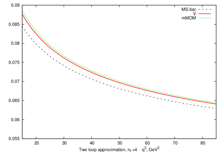
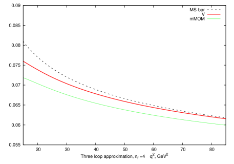
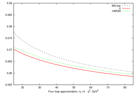
Figure 1: Scheme dependence of the NLO (left), NNLO (right) and N³LO (bottom) approximations for the e${}^{+}e^{-}$ characteristic $r(q^{2})=R(q^{2})/(3\sum_{f}Q^{2}_{f})-1$ in the case of $n_{f}$=4 numbers of active flavours. The dashed black curve depicts the variations of the ${\rm{\overline{MS}}}$ approximants. The solid (green) line demonstrate the variations of the ${\rm{mMOM}}$-scheme results, while the solid red line shows the V-scheme results.

In the numerical form the expressions for the $\rm{\overline{MS}}$ $\beta$-functions coefficients $\beta_{i}$ in Eqs. (72)-(76) are defined in Eqs. (35), (36) and Eqs.(56),(57) respectively. For the concrete numbers of $n_{f}$ flavours their values are given in Table 1. Note that in the analysis of Ref.Gracey:2014pba the same expansion was used for the numbers of active flavours $n_{f}$=$5$ and $n_{f}$=$6$ and for the value of $\Lambda_{\rm{\overline{MS}}}=500$ MeV, which did not vary from order to order of the $\rm{\overline{MS}}$-scheme perturbative expressions considered in Ref. Gracey:2014pba . In the process of obtaining our results, presented in Figs. 1 and 2, and keeping in mind physical motivations, discussed above, we used $n_{f}$=$4$ and $n_{f}$=$5$.

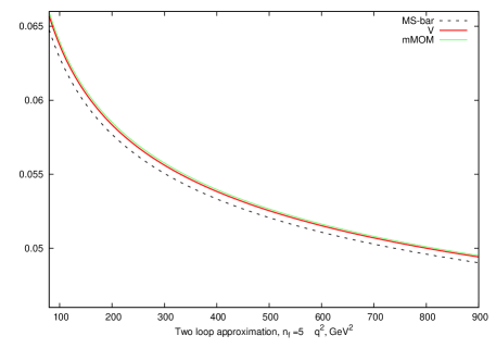
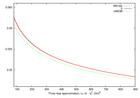
Figure 2: Scheme dependence of the NLO (left), NNLO (right) and N³LO (bottom) approximations to $r(q^{2})$ are presented for $n_{f}$=$5$ numbers of active flavours. The variation of the ${\rm{\overline{MS}}}$-, mMOM- and V-scheme results is indicated by the three curves as in Fig.1

Contrary to the studies of Ref. Gracey:2014pba the values of the parameters $\Lambda^{(n_{f})}_{\rm{\overline{MS}}}$ , $\Lambda^{(n_{f})}_{\rm{mMOM}}$ and parameter $\Lambda^{(n_{f})}_{\rm{V}}$ (that is new to this work) were not fixed, but depend on the choice of both $n_{f}$ and the order of approximations. The concrete results for the values of the parameters used are presented in Table 3.

The numerical values of the $\Lambda_{\rm{QCD}}$ in different schemes, MeV
$n_{f}$	the order of approximation $\nu$	$\Lambda^{(n_{f})}_{\overline{\rm{MS}}}$	$\Lambda^{(n_{f})}_{\rm{V}}$	$\Lambda^{(n_{f})}_{\rm{mMOM}}$
4	2	350	500	625
4	3	335	475	600
4	4	330	470	590
5	2	250	340	435
5	3	245	335	430
5	4	240	330	420

Table 3. The dependence of the parameters, used for getting the results of Figs. 1 and 2 from the $n_{f}$, $\nu$ (order of approximation), and from the choice of the scheme.

In the cases of $n_{f}$=$4$ numbers of active flavours and $\nu=2,3,4$ the values for $\Lambda^{(n_{f}=4)}_{\rm{\overline{MS}}}$ given in Table 3 are fixed from the results of the fits fits of the Fermilab Tevatron experimental data for the $xF_{3}$ structure function of the neutrino-nucleon deep-inelastic scattering process at the $\rm{N^{(\nu-1)}LO}$ of the theoretical PT results, performed in Ref.Kataev:2001kk . In the case of $n_{f}=5$ the values of $\Lambda^{(n_{f}=5)}_{\rm{\overline{MS}}}$ at $\nu=2,3,4$ were obtained in Ref. Kataev:2009ns from the related results for $\Lambda^{(n_{f}=4)}_{\rm{\overline{MS}}}$ using the the NLO, NNLO and $\rm{N^{3}LO}$ matching conditions, evaluated at the NNLO in Ref. Bernreuther:1981sg and Larin:1994va and at the $\rm{N^{3}LO}$ in Ref. Chetyrkin:1997sg . The matching point in these conditions was fixed by the on-shell b-quark mass values, extracted at different orders of PT from the analysis of heavy quarkonium spectrum while taking into account the Pade estimated value of the coefficient $a_{3}$ from Eq. (13), obtained in Ref. Chishtie:2001mf . These Pade estimates turned out to be in satisfactory agreement with the results of direct calculations of the value of $a_{3}$ obtained later (see Refs. Smirnov:2008pn , Smirnov:2009fh , Anzai:2009tm ). In view of reliability of the results of Ref. Penin:2002zv we may safely use the values for $\Lambda^{(n_{f}=5)}_{\rm{\overline{MS}}}$ from Table 3 for transforming them to the values of the scale parameters $\Lambda^{(n_{f}=5)}_{\rm{mMOM}}$ and $\Lambda^{(n_{f}=5)}_{\rm{V}}$ in particular.

In general the scale parameters $\Lambda^{(n_{f})}$ of the $\rm{\overline{MS}}$ , V and $\rm{mMOM}$ schemes considered in Table 3 are related by the following equations:

$$\Lambda^{{(n_{f})}2}_{\rm{V}}=\Lambda^{{(n_{f})}2}_{\overline{\rm{MS}}}\rm{exp}[a^{\overline{\rm{MS}}}_{1}(n_{f})/\beta_{0}(n_{f})]~{},~{}\Lambda^{{(n_{f})}2}_{\rm{mMOM}}=\Lambda^{{(n_{f})}2}_{\overline{\rm{MS}}}\rm{exp}[(r^{\overline{\rm{MS}}}_{1}(n_{f})-r^{\rm{mMOM}}_{1}(n_{f}))/4\beta_{0}(n_{f})]~{}.$$ (77)

They are derived by means of the ECH approach. We used these expressions to get in Table 3 the numerical values of $\Lambda^{(n_{f})}_{\rm{V}}$ and $\Lambda^{(n_{f})}_{\rm{mMOM}}$ from the results described above for $\Lambda^{(n_{f})}_{\overline{\rm{MS}}}$. Combining them with the numerical values for the coefficients $\beta_{2}^{\rm{V}}(n_{f})$ , $\beta_{3}^{\rm{V}}(n_{f})$ and $\beta^{\rm{mMOM},\lambda=0}_{2}(n_{f})$ , $\beta^{\rm{{mMOM},\lambda=0}}_{3}(n_{f})$ in the analogs of Eqs. (72), (74) and Eq.(76), and taking into account the expressions for the coefficients $r_{i}$ in $r(q^{2})=R(q^{2})/(3\sum_{f}Q^{2}_{f})-1$ in three different schemes, we plot in Figs.1 and 2 the energy dependence of $r(q^{2})$ in three different orders of PT and three different schemes, namely $\rm{\overline{MS}}$, V and mMOM schemes in the case of $n_{f}=4$ and $n_{f}=5$ respectively.

IV.6 Discussions of the results.

Considering now the plots of Figs.1 and 2 we may conclude that in all cases the PT approximants for the function $r(s)$ related to the $e^{+}e^{-}$-annihilation R-ratio are converging in all schemes. In the $\rm{\overline{MS}}$ scheme the rate of convergence of the related PT approximants is better than in the V scheme and mMOM scheme. At the NLO the results of the V scheme are closer to the mMOM ones than to the results obtained in $\rm{\overline{MS}}$ scheme, while at the NNLO the situation is reversed – the V-scheme approximations are closer to the $\rm{\overline{MS}}$-ones, while the application of the mMOM scheme puts a lower bound on the theoretical expression for $r(s)$. However, at the N³LO the lower theoretical bound on the energy dependence of $r(s)$ is changed again and the lower bound is now obtained within V scheme. The comparison of three approximants for $r(s)$ in the case of consideration of the V-sche me results supports the conclusion, made in Sec. IV. C, that the PT approximants in the V scheme have less regular behaviour than the $\rm{\overline{MS}}$ ones. The results of Table 2 demonstrate the positive feature of taking into account $O(\alpha_{s}^{4})$-corrections to $e^{+}e^{-}$ annihilation R-ratio in all three schemes. Indeed, the scheme dependence of the expression for the $e^{+}e^{-}$ ratio is drastically decreased at this level. This is the positive message, which supports the work presented above on the inclusion of the $O(\alpha_{s}^{4})$ correction in the theoretical approximations in the $\rm{\overline{MS}}$, mMOM and V schemes.

V The four-loop QED result for the RG $\beta$ function in the $\rm{V}$ scheme

Consider now the case of QED with N types of identically charged leptons. We will use the results of Sec. III.2 for the the fourth-order PT approximation of the RG $\rm{V}$-scheme $\beta$-function of the $SU(N_{c})$ colour gauge group theory. Fixing the $SU(N_{c})$ group weights in Eqs. (31), (32), (III.2) and (III.2) as $C_{A}=0$, $C_{F}=1$, $T_{F}=1$, $d^{abcd}_{A}=0$, $d^{abcd}_{F}=1$, $N_{A}=1$ and $n_{f}=N$, we obtain the following four-loop semi-analytical expression for the RG $\beta$ function in QED in the ${\rm V}$ scheme:

$$\beta^{\rm{V}}_{QED}(a_{V})=\frac{4}{3}Na_{\rm{V}}^{2}+4Na_{\rm{V}}^{3}+\bigg{(}-2N+(\frac{64}{3}\zeta(3)-\frac{184}{9})N^{2}\bigg{)}a_{\rm{V}}^{4}+$$

$$+ \bigg{(}-46N+(104+\frac{512}{3}\zeta(3)-\frac{1280}{3}\zeta(5)-\frac{8}{3}\cdot 56.83(1))N^{2}+(128-\frac{256}{3}\zeta(3))N^{3}\bigg{)}a_{\rm{V}}^{5}+O(a_{\rm{V}}^{6})$$

where $a_{\rm{V}}=\alpha_{\rm{V}}/4\pi$ and $N$ is the number of leptons. Comparing this result with the four-loop approximation of the QED $\beta$ function in the MOM scheme, i. e. of the Gell-Man–Low $\Psi$ function, namely with

$$\Psi(a_{\rm{MOM}})=\frac{4}{3}Na_{\rm{MOM}}^{2}+4Na_{\rm{MOM}}^{3}+\bigg{(}-2N+(\frac{64}{3}\zeta(3)-\frac{184}{9})N^{2}\bigg{)}a_{\rm{MOM}}^{4}$$

$$+ \bigg{(}-46N+(104+\frac{512}{3}\zeta(3)-\frac{1280}{3}\zeta(5))N^{2}+(128-\frac{256}{3}\zeta(3))N^{3}\bigg{)}a_{\rm{MOM}}^{5}+O(a_{\rm{MOM}}^{6})$$

where $a_{\rm{MOM}}=\alpha_{\rm{MOM}}/4\pi$, we conclude that in spite of identical agreement at the third order of PT , the general expressions for the RG QED $\beta$ function in these two different schemes are not the same. They start to differ from the fourth order of PT due to contributing to the $O(a_{\rm{V}}^{5})$ coefficient of the $\beta^{\rm{V}}$-function of the additional light-by-light-type scattering diagrams, which appear in the QED analog of the coefficient $a_{3}^{(1)}$ in the $\rm{\overline{MS}}$ scheme, given in Eq. (II). They enter in the definition of the $N^{2}$-term of the $\beta_{3}^{\rm{V}}$ coefficient of the V-scheme QED $\beta$-function through Eq. (30).

It is possible to clarify what kind of N-dependent high-order coefficients of the following expression of the QED $\beta$ function in the V scheme

$$\beta^{\rm{V}}(a_{\rm{V}})=\sum\limits_{i=0}^{\infty}\beta_{i}^{\rm{V}}\bigg{(}\frac{\alpha_{{\rm{V}}}}{4\pi}\bigg{)}^{i+2}=\beta^{\rm{V}[1]}_{0}N\bigg{(}\frac{\alpha_{{\rm{V}}}}{4\pi}\bigg{)}^{2}+\sum\limits_{i=1}^{\infty}\sum\limits_{l=1}^{i}\beta^{\rm{V}[l]}_{i}N^{l}\bigg{(}\frac{\alpha_{{\rm{V}}}}{4\pi}\bigg{)}^{i+2}$$ (80)

will also receive additional contributions and what kind of the N-dependent coefficients of the QED $\beta^{\rm{V}}$ function will coincide with the similar expressions for the $\Psi$ function, which we will define as

$$\Psi(a_{\rm{MOM}})=\Psi^{[1]}_{0}N\bigg{(}\frac{\alpha_{\rm{MOM}}}{4\pi}\bigg{)}^{2}+\sum\limits_{i=1}^{\infty}\sum\limits_{l=1}^{i}\Psi^{[l]}_{i}N^{l}\bigg{(}\frac{\alpha_{\rm{MOM}}}{4\pi}\bigg{)}^{i+2}.$$ (81)

Using the analogs of Eq. (29) and (30), which can be derived using the considerations of Ref. Kataev:1995vh , we arrive at the following relations:

$$\beta_{i}^{{\rm{V}[l]}}=\Psi_{i}^{[l]}+\Delta\beta_{i}^{{\rm{V}[l]}}$$ (82)

where extra terms $\Delta\beta_{i}^{{\rm{V}[l]}}$ in the N-dependent contributions to the coefficients of the QED $\beta^{V}$ function appear in the following region of indexes $[i,l]=[i\geq 3,2\leq l\leq i-1]$.

In the cases of $[i,l]=[i\geq 3,l=1~{}\text{or}~{}i]$ the proportional to $N^{[l]}$ coefficients of the $\beta^{\rm{V}}$ and $\Psi$ function, defined in Eq. (80) and (81), are the same. In the case of i=3, which corresponds to the totally known for the moment fourth order results, these identical coefficients are proportional to N and $N^{3}$. At the third order the proportional to N-term was analytically evaluated in Ref. (Rosner:1967zz, ). At the fourth order of PT the proportional to N and $N^{3}$ terms were evaluated in Ref. (Gorishnii:1990kd, ). For $i=4$ the terms under discussion can be obtained from the results of Ref.Baikov:2012zm and read

$$\beta_{4}^{{\rm{V}[1]}}=\Psi_{4}^{[1]}=\frac{4157}{6}+128\zeta(3)$$ (83)

$$\beta_{4}^{{\rm{V}[4]}}=\Psi_{4}^{[4]}=-\frac{8756}{9}+\frac{3584}{9}\zeta(3)+\frac{5120}{9}\zeta(5)$$ (84)

Note that this result from Ref. Baikov:2012zm is in agreement with the multiloop expression for this particular contribution to the Gell-Man–Low function, evaluated in Ref. Broadhurst:1992si up to 20 loops analytically and numerically up to 100 loops. The scheme-independence of the linear-in-N-contribution to Eqs. (80) and (81) is the consequence of the conformal symmetry property, which is valid in QED in the perturbative quenched approximation (for the recent detailed study see Ref. Kataev:2013vua ).

In the numerical form the scheme-dependent coefficients of the $\beta^{V}_{\rm{QED}}$-function read:

$$\beta_{2}^{\rm{V}} = -2N+5.19943N^{2}$$ (85)

$$\beta_{3}^{\rm{V}} = -46N+284.818(26)N^{2}-25.42447N^{3}$$ (86)

The analogous expressions for the three- and four-loop coefficients of the QED $\beta$ function in the $\overline{\rm{MS}}$ scheme follow from the analytical results of Ref. Gorishnii:1990kd and have the following form

$$\beta_{2}^{\overline{\rm{MS}}} = -2N+4.88888N^{2}$$ (87)

$$\beta_{3}^{\overline{\rm{MS}}} = -46N+82.9753N^{2}+5.06995N^{3}$$ (88)

The numerical expressions for the analogous coefficients of the $\Psi$ function (or the QED $\beta$ function in MOM scheme), which we obtain from the same work of Ref. Gorishnii:1990kd , are

$$\Psi_{2} = -2N+5.19943N^{2}$$ (89)

$$\Psi_{3} = -46N+133.2714N^{2}-25.42447N^{3}$$ (90)

Note once more that the first three coefficients of the $\beta^{\rm{V}}$ function and of the $\Psi$ function are the same and start to differ from the fourth order of PT in the following way

$$\beta_{3}^{\rm{V}}=\Psi_{3}-151.54(2)N^{2}$$ (91)

This additional contribution arises from the light-by-light-type scattering contribution, which is typical to the V scheme.

For completeness we present the QED expressions for the $O(\alpha^{5})$ approximations for the $\Psi$ and $\beta^{V}_{QED}$ functions in the case of N=1 :

$$\Psi(a_{\rm{MOM}}) = 1.3333a_{\rm{MOM}}^{2}+4a_{\rm{MOM}}^{3}+3.1994a_{\rm{MOM}}^{4}-153.8469a_{\rm{MOM}}^{5}+O(a_{\rm{MOM}}^{6})$$ (92)

$$\beta^{V}_{QED}(a_{\rm{v}}) = 1.3333a_{\rm{V}}^{2}+4a_{\rm{V}}^{3}+3.1994a_{\rm{V}}^{4}-305.3936(266)a_{\rm{V}}^{5}+O(a_{\rm{V}}^{6})$$ (93)

One can observe that even for N=1 the numerical effect of light-light-scattering contribution, which is typical for the V-scheme (see Eq. (91) ), is rather sizable and almost equals to the whole value of the other term in the expression of Eq. (91).

VI Conclusion

In this work we consider the definition of the gauge-independent RG QCD $\beta$ function in the $\rm{V}$ scheme. Using higher-order corrections to the static potential of the quark-antiquark interaction and $\beta$ function in $\overline{\rm{MS}}$ scheme, we compute the fourth term of the PT expression for the $\beta$ function in $\rm{V}$ scheme in the general case of $\rm{SU(N_{c})}$ group in the semi-analytical term. Our guess of possible expressions of the corresponding numerical contributions through concrete transcendental numbers is made. The comparison of the numerical expressions of the scheme-dependent coefficients of the $\beta^{\rm{V}}$ function of QCD with the similar coefficients of the QCD $\beta$ function in the $\rm{\overline{MS}}$ and $\rm{mMOM}$ scheme in the Landau gauge are presented. The indication that the structure of the PT series for the effective $\beta$ function in the $\rm{V}$ scheme has non-regular asymptotic behaviour and differs from the asymptotic PT for the $\beta$ function in the $\rm{\overline{MS}}$ scheme are presented. The results obtained in the V scheme are used to study the scheme dependence of the $O(\alpha_{s}^{4})$ approximation for the $e^{+}e^{-}$ annihilation R-ratio in the energy region above the thresholds of production of the charmonium states. The conclusion is made that the comparison between the fourth-order expressions for the $e^{+}e^{-}$ annihilation R-ratio, obtained in the $\rm{\overline{MS}}$ schemes, in the Landau-gauge variant of the mMOM scheme and in the gauge-independent V scheme leads to a drastic decrease of the scheme dependence of the fourth-order perturbative QCD predictions for the case of $n_{f}=5$ numbers of active flavours in particular. Considering the QED limit of the $\rm{SU(N_{c})}$-group $\beta^{\rm{V}}$ function we observe that its perturbative expression is starting to differ from the perturbative expression for the Gell-Mann–Low $\Psi$ function from the level of the $O(\alpha_{\rm{V}}^{6})$-corrections. The relations between coefficients of the QED $\beta^{\rm{V}}$ function and the $\Psi$ function are presented in all orders of PT in the case of the N-types of identical leptons. The conclusion that starting from the fourth-order perturbative approximation two N-dependent terms in the coefficients of the perturbative expansions of the $\beta^{\rm{V}}$ and $\Psi$ functions will always coincide is made. Theoretical reasons of this foundations are presented.

- (1) E. C. G. Stueckelberg and A. Petermann, Helv. Phys. Acta 26 499 (1953).
- (2) N. N. Bogolyubov and D. V. Shirkov, Nuovo Cim. 3 845 (1956) .
- (3) M. Gell-Mann and F. E. Low, Phys. Rev. 95 1300 (1954).
- (4) R. Jost and J.M. Luttinger, Helv. Phys. Acta 23 201 (1950) .
- (5) N. N. Bogolyubov and D. V. Shirkov, “Introduction To The Theory of Quantized Fields,”, Moscow, Nauka, 1984; Intersci. Monogr. Phys. Astron. 3 1 (1959).
- (6) M. Baker and K. Johnson, Phys. Rev. 183 1292 (1969).
- (7) S. G. Gorishny, A. L. Kataev and S. A. Larin, Phys. Lett. B 194 429 (1987).
- (8) S. G. Gorishny, A. L. Kataev, S. A. Larin and L. R. Surguladze, Phys. Lett. B 256 81 (1991).
- (9) P. A. Baikov, K. G. Chetyrkin, J. H. Kuhn and J. Rittinger, JHEP 07 (2012) 017.
- (10) A. L. Kataev and S. A. Larin, Pisma Zh. Eksp. Teor. Fiz. 96 64 (2012) [JETP Lett. 96 61 (2012)].
- (11) E. De Rafael and J. L. Rosner, Annals Phys. 82 369 (1974).
- (12) D. J. Broadhurst, A. L. Kataev and O. V. Tarasov, Phys. Lett. B 298 445 (1993).
- (13) P. A. Baikov, K. G. Chetyrkin, J. H. Kuhn and C. Sturm, Nucl. Phys. B 867 182 (2013).
- (14) G. ’t Hooft and M. J. G. Veltman, Nucl. Phys. B 44 189 (1972).
- (15) G. ’t Hooft, Nucl. Phys. B 61 455 (1973).
- (16) W. A. Bardeen, A. J. Buras, D. W. Duke and T. Muta, Phys. Rev. D 18 3998 (1978).
- (17) K. G. Chetyrkin, A. L. Kataev and F. V. Tkachov, Nucl. Phys. B 174 345 (1980).
- (18) A. A. Vladimirov, Theor. Math. Phys. 43 417 (1980) [Teor. Mat. Fiz. 43 210 (1980)].
- (19) A. A. Vladimirov and D. V. Shirkov, Sov. Phys. Usp. 22 860 (1979) [Usp. Fiz. Nauk 129 407 (1979)].
- (20) D. J. Gross and F. Wilczek, Phys. Rev. Lett. 30 1343 (1973).
- (21) H. D. Politzer, Phys. Rev. Lett. 30 1346 (1973).
- (22) D. R. T. Jones, Nucl. Phys. B 75 531 (1974).
- (23) W. E. Caswell, Phys. Rev. Lett. 33 244 (1974).
- (24) E. Egorian and O. V. Tarasov, Teor. Mat. Fiz. 41 26 (1979) [Theor. Math. Phys. 41 863 (1979)].
- (25) A. A. Belavin and A. A. Migdal, Pisma Zh. Eksp. Teor. Fiz. 19 317 (1974).
- (26) O. V. Tarasov, A. A. Vladimirov and A. Y. Zharkov, Phys. Lett. B 93 429 (1980).
- (27) S. A. Larin and J. A. M. Vermaseren, Phys. Lett. B 303 334 (1993).
- (28) T. van Ritbergen, J. A. M. Vermaseren and S. A. Larin, Phys. Lett. B 400 379 (1997).
- (29) M. Czakon, Nucl. Phys. B 710 485 (2005).
- (30) D. I. Kazakov and V. S. Popov, JETP Lett. 77 453 (2003) [Pisma Zh. Eksp. Teor. Fiz. 77 547 (2003)].
- (31) M. Peter, Phys. Rev. Lett. 78 602 (1997).
- (32) Y. Schroder, Phys. Lett. B 447 321 (1999).
- (33) S. J. Brodsky, M. Melles and J. Rathsman, Phys. Rev. D 60 096006 (1999).
- (34) D. J. Broadhurst, A. L. Kataev and C. J. Maxwell, Nucl. Phys. B 592 247 (2001).
- (35) L. von Smekal, K. Maltman and A. Sternbeck, Phys. Lett. B 681 336 (2009).
- (36) J. A. Gracey, Phys. Rev. D 90 9, 094026 (2014).
- (37) A. Pineda and F. J. Yndurain, Phys. Rev. D 61 077505 (2000).
- (38) C. Ayala, G. Cvetic and A. Pineda, JHEP 09 045 (2014).
- (39) Y. Kiyo and Y. Sumino, Nucl. Phys. B 889 156 (2014).
- (40) T. van Ritbergen, A. N. Schellekens and J. A. M. Vermaseren, Int. J. Mod. Phys. A 14 41 (1999).
- (41) W. Fischler, Nucl. Phys. B 129 157 (1977).
- (42) A. Billoire, Phys. Lett. B 92 343 (1980).
- (43) A. V. Smirnov, V. A. Smirnov and M. Steinhauser, Phys. Lett. B 668 293 (2008).
- (44) S. G. Gorishny, A. L. Kataev and S. A. Larin, Phys. Lett. B 273 141 (1991) [Erratum-ibid. B 275 512 (1992)] .
- (45) A. V. Smirnov, V. A. Smirnov and M. Steinhauser, Phys. Rev. Lett. 104 112002 (2010).
- (46) C. Anzai, Y. Kiyo and Y. Sumino, Phys. Rev. Lett. 104 112003 (2010).
- (47) B. A. Kniehl, A. A. Penin, V. A. Smirnov and M. Steinhauser, Nucl. Phys. B 635 357 (2002).
- (48) T. Appelquist, M. Dine and I. J. Muzinich, Phys. Rev. D 17 2074 (1978).
- (49) N. Brambilla, A. Pineda, J. Soto and A. Vairo, Phys. Rev. D 60 091502 (1999). .
- (50) G. Grunberg, Phys. Lett. B 95 70 (1980) [Erratum-ibid. B 110 501 (1982)].
- (51) G. Grunberg, Phys. Rev. D 29 2315 (1984).
- (52) N. V. Krasnikov, Nucl. Phys. B 192 497 (1981) .
- (53) A. L. Kataev, N. V. Krasnikov and A. A. Pivovarov, Nucl. Phys. B 198 508 (1982) [Erratum-ibid. B 490 505 (1997)] .
- (54) W. Celmaster and R. J. Gonsalves, Phys. Rev. D 20 1420 (1979).
- (55) E. Braaten and J. P. Leveille, Phys. Rev. D 24 1369 (1981).
- (56) A. Dhar and V. Gupta, Phys. Lett. B 101 432 (1981).
- (57) P. A. Raczka and R. Raczka, Phys. Rev. D 39 643 (1989).
- (58) O. V. Tarasov and D. V. Shirkov, Sov. J. Nucl. Phys. 51 877 (1990) [Yad. Fiz. 51 1380 (1990)].
- (59) K. G. Chetyrkin and A. Retey, hep-ph/0007088.
- (60) K. G. Chetyrkin and T. Seidensticker, Phys. Lett. B 495 74 (2000).
- (61) J. A. Gracey, Phys. Lett. B 700 79 (2011).
- (62) J. A. Gracey, J. Phys. A 46 225403 (2013).
- (63) P. M. Stevenson, Phys. Rev. D 23 2916 (1981).
- (64) A. L. Kataev and V. V. Starshenko, Mod. Phys. Lett. A 10 235 (1995).
- (65) T. A. Ryttov, Phys. Rev. D 89 5, 056001 (2014).
- (66) R. Shrock, Phys. Rev. D 89 4, 045019 (2014).
- (67) J. A. Gracey and R. M. Simms, Phys. Rev. D 91 8, 085037 (2015)
- (68) P. A. Raczka and R. Raczka, Phys. Rev. D 40 878 (1989).
- (69) S. G. Gorishny, A. L. Kataev and S. A. Larin, Phys. Lett. B 212 238 (1988).
- (70) S. G. Gorishny, A. L. Kataev and S. A. Larin, Phys. Lett. B 259 144 (1991).
- (71) L. R. Surguladze and M. A. Samuel, Phys. Rev. Lett. 66 560 (1991) [Erratum-ibid. 66 2416 (1991)].
- (72) K. G. Chetyrkin, Phys. Lett. B 391, 402 (1997).
- (73) P. A. Baikov, K. G. Chetyrkin and J. H. Kuhn, Phys. Rev. Lett. 101 012002 (2008).
- (74) P. A. Baikov, K. G. Chetyrkin, J. H. Kuhn and J. Rittinger, Phys. Lett. B 714 62 (2012).
- (75) J. Greensite, A. V. Kovalenko, S. Olejnik, M. I. Polikarpov, S. N. Syritsyn and V. I. Zakharov, Phys. Rev. D 74 094507 (2006).
- (76) I. M. Suslov, Zh. Eksp. Teor. Fiz. 127 1350 (2005) [J. Exp. Theor. Phys. 100 1188 (2005)] [hep-ph/0510142].
- (77) L. N. Lipatov, Sov. Phys. JETP 45 216 (1977) [Zh. Eksp. Teor. Fiz. 72 411 (1977)].
- (78) S. J. Brodsky and H. J. Lu, Phys. Rev. D 51, 3652 (1995).
- (79) K. G. Chetyrkin, A. L. Kataev and F. V. Tkachov, Phys. Lett. B 85, 277 (1979).
- (80) M. Dine and J. R. Sapirstein, Phys. Rev. Lett. 43, 668 (1979).
- (81) W. Celmaster and R. J. Gonsalves, Phys. Rev. Lett. 44, 560 (1980).
- (82) K. G. Chetyrkin, B. A. Kniehl and M. Steinhauser, Phys. Rev. Lett. 79, 2184 (1997)
- (83) A. L. Kataev, G. Parente and A. V. Sidorov, Phys. Part. Nucl. 34, 20 (2003) [Fiz. Elem. Chast. Atom. Yadra 34, 43 (2003)] Erratum: ibid. 38, no. 6, 827 (2007) [hep-ph/0106221].
- (84) A. L. Kataev and V. T. Kim, PoS ACAT 08, 004 (2008) [arXiv:0902.1442 [hep-ph]].
- (85) W. Bernreuther and W. Wetzel, Nucl. Phys. B 197, 228 (1982) [Nucl. Phys. B 513, 758 (1998)].
- (86) S. A. Larin, T. van Ritbergen and J. A. M. Vermaseren, Nucl. Phys. B 438, 278 (1995) [hep-ph/9411260].
- (87) F. A. Chishtie and V. Elias, Phys. Lett. B 521, 434 (2001)
- (88) A. A. Penin and M. Steinhauser, Phys. Lett. B 538, 335 (2002)
- (89) A. V. Garkusha, Master Thesis of Math. Dep. of High School of Economics (2013) (unpublished).
- (90) J. L. Rosner, Annals Phys. 44, 11 (1967).
- (91) D. J. Broadhurst, Z. Phys. C 58, 339 (1993).
- (92) A. L. Kataev, JHEP 02, 092 (2014)