Corresponding states law for a generalized Lennard-Jones potential

Abstract

It was recently shown that vapor-liquid coexistence densities derived from Mie and Yukawa models collapse to define a single master curve when represented against the difference between the reduced second virial coefficient at the corresponding temperature and that at the critical point. In this work we further test this proposal for another generalization of the Lennard-Jones pair potential. This is carried out for vapor-liquid coexistence densities, surface tension, and vapor pressure, along a temperature window set below the critical point. For this purpose we perform molecular dynamics simulations by varying the potential softness parameter to produce from very short to intermediate attractive ranges. We observed all properties to collapse and yield master curves. Moreover, the vapor-liquid curve is found to share the exact shape of the Mie and attractive Yukawa. Furthermore, the surface tension and the logarithm of the vapor pressure are linear functions of this difference of reduced second virial coefficients.

I Introduction

Leaving aside conformal pair potentials (those which are invariant by rescaling distance and energy and for which the corresponding states law is strictly valid Pitzer (1939)), the classic van der Waals framework works relatively well for defining master curves for thermodynamic properties derived from pair potential shapes of variable attractive range Okumura and Yonezawa (2000); Dunikov et al. (2001); Orea et al. (2008); Galliero et al. (2009); Blas et al. (2012a, b); Chapela et al. (2013); Martínez-Valencia et al. (2013); Patra et al. (2012) and real systems Katsonis et al. (2006); Valadez-Pérez et al. (2012); Román et al. (2005); Weiss and Schröer (2007); Galliero (2010); Wei et al. (2013); Mousazadeh et al. (2006); Castellanos et al. (2004); Ghatee et al. (2002); Puosi and Leporini (2011); Boire et al. (2013). This quasiuniversality, together with the Lindemann melting criterion Ubbelohde (1965), the so-called excess-entropy scaling of liquid’s relaxation times and diffusion coefficients Rosenfeld (1977), among other approximate corresponding states features Young and Andersen (2003); Galliero et al. (2007); Galliero and Boned (2008), has lead to discover that many liquids and solids have an approximate hidden scale invariance, implying the existence of isomorph lines in the thermodynamic phase diagram along which reduced structure and dynamic properties are invariant to a good approximation Bacher et al. (2014); Dyre (2014). In other words, the phase diagram becomes one-dimensional with regard to several physical properties.

In line with this scale invariance, quite recently we have observed that a slight modification of the extended law of corresponding states Noro and Frenkel (2000) is capable of improving the output of the van der Waals framework for the Mie and attractive Yukawa expressions (which are non-conformal potential functions) Orea et al. (2015). Results have shown that this proposal not only improve the Mie and Yukawa data collapse but the obtained master curves were indistinguishable. Hence the following questions naturally raise: Is this framework general, leading always to data collapses for spherically symmetric potentials? Are the Mie and Yukawa the only functional shapes sharing a master curve for the vapor-liquid coexistence? Are the vapor-liquid coexistence densities the only properties showing this general behavior? This work can be seen as an effort to answer, at least partially, these questions.

The extended law of corresponding states Noro and Frenkel (2000) was derived as an attempt to generalize the classic van der Waals principle Pitzer (1939); Guggenheim (1945) to non-conformal potentials, in particular for pair potentials of variable attractive range. This, in view that the nature of colloidal interactions show such character Hunter (2001). For this purpose, Noro and Frenkel suggested including the reduced second virial coefficient, $B_{2}^{*}$, as an additional independent variable which is clearly linked to the attractive range Noro and Frenkel (2000). This is justified since the value of $B_{2}^{*}$ at the critical point is frequently close to $-1.5$ for several non-conformal potentials Vliegenthart and Lekkerkerker (2000). Nonetheless, small deviations from this particular value have an undesirable impact on the definition of master curves for all properties. Hence, we proposed $B_{2s}=B_{2}^{*}(T^{*})-B_{2}^{*}(T^{*}_{c})$ as the additional independent variable instead (being $T^{*}_{c}$ the dimensionless critical temperature) Orea et al. (2015).

In this work we are testing the performance of this framework for another continuous non-conformal potential shape. This is the so-called Approximate Non-Conformal (ANC) potential del Río et al. (2005), which can be seen as a generalization of the Lennard-Jones model or even a generalization of a spherically symmetric Kihara Kihara (1954). The ANC expression provides a family of potential functions that accurately give the dilute vapor phase properties of several real substances McLure et al. (1999); del Río et al. (2007, 2013). The potential allows the tuning of its (and attractive range) by varying a single parameter, $s$. It has also the advantage of showing an analytical second virial coefficient González-Calderón and Rocha-Ichante (2015). Its spherical symmetry and non-conformal character make it appropriate for our purpose. Hence, we perform molecular dynamics simulations (using the Gromacs package van der Spoel et al. (2005); Hess et al. (2008)) to obtain vapor-liquid coexistence densities, surface tension, and vapor pressure for this particular functional shape. These data allow us to build master curves for the three properties as tentative universal forms. In fact, we corroborate the shape obtained in previous work for the vapor-liquid densities Orea et al. (2015). It is also shown that this slight modification of the Noro and Frenkel extended law of corresponding states Noro and Frenkel (2000) is capable of producing striking data collapses of several properties when varying the potential range, and leads to really simple relationships between several properties and $B_{2s}$. Capturing a universal behavior (independence of the properties on the details and range of the pair-potential function) is important in the soft matter field since colloidal interactions strongly depend on the composition of both phases, continuous and dispersed Hunter (2001).

The manuscript is structured as follows. After this brief introduction we present in section II the model potential and the methods employed for obtaining the vapor-liquid coexistence densities, vapor pressure, surface tension, and critical properties. Section III shows the raw results and the outcomes from both, the classic van der Waals and the extended frameworks. Here we give simple expressions for the vapor pressure and the surface tension master curves. Finally, section IV presents the more relevant conclusions.

II Model and method

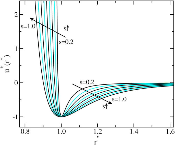
Figure 1: Pair potential $u^{*}(r^{*})$ as a function of the softness parameter, $s$. Parameter $s$ increases from 0.2 to 1.0 in steps of 0.1. Arrows point to the direction of increasing $s$. A larger $s$ value leads to a softer curve and a longer interaction range.

In reduced units ($u^{*}=u/\varepsilon$, being $\varepsilon$ the potential well depth) the ANC pair potential is given by del Río et al. (1998)

$$u^{*}(r^{*})=\left[\frac{1-a}{\xi(r^{*})-a}\right]^{12}-2\left[\frac{1-a}{\xi(r^{*})-a}\right]^{6}{,}$$ (1)

where $a=0.09574$ is a constant, $r^{*}$ is the dimensionless distance $r^{*}\equiv r/r_{m}$, $r_{m}$ is the distance at which the potential reaches its minimum,

$$\xi(r^{*})=\left(\frac{r^{*3}-1}{s}+1\right)^{1/3},$$

and $s$ is the so called softness parameter. For $s=1$, equation 1 produces a spherically symmetric Kihara with hard-core diameter $a$. On the other hand, for the fixed value of $a$, $s=1.13$ approaches the Lennard-Jones interaction  del Río et al. (2005, 2007) (the ANC leads to the exact Lennard-Jones interaction for $a=0$ and $s=1$). The effect of $s$ on the shape of the potential is shown in figure 1. Note that expression 1 works properly for inter-particle distances above $r^{*}_{s}=(s(a^{3}-1)+1)^{1/3}$. For $r^{*}\leq r^{*}_{s}$ we are setting $u^{*}(r^{*})=u^{*}(r^{*}_{s})$, being for all cases $u^{*}(r^{*}_{s})$ a very large positive value (the value of $u^{*}(r^{*})$ for $r^{*}<r^{*}_{s}$ is indeed irrelevant). Along the manuscript we are using $\rho^{*}=\rho r_{m}^{3}$ as unit of density (being $\rho$ the number density), $T^{*}=k_{B}T/\varepsilon$ (being $k_{B}$ the Boltzmann constant), $\gamma^{*}=\gamma r_{m}^{2}/\varepsilon$, $P^{*}=Pr_{m}^{3}/\varepsilon$, and $t^{*}=t\sqrt{\varepsilon/mr_{m}^{2}}$ ($m$ is the particle mass).

This potential is tabulated to be used as input for the Gromacs molecular dynamics package van der Spoel et al. (2005); Hess et al. (2008). We are performing $NVT$ replica exchange simulations expanding the ensemble in temperature Lyubartsev et al. (1992); Marinari and Parisi (1992). The velocity rescale algorithm is employed as thermostat Bussi et al. (2007). The step time is set to $dt^{*}=0.001$ (except for the case with $s=0.2$ which is $dt^{*}=0.0005$). The cutoff distance, $r_{c}$, for tables and neighbor list searching is such that $|u^{*}(r_{c})|<10^{-4}$ for all cases. We are considering a simulation cell having a rectangular parallelepiped shape with $L_{x}=L_{y}=9r_{m}$ and $L_{z}=30r_{m}$ for $s<0.7$ and with $L_{x}=L_{y}=10r_{m}$ for the cases having $s\geq 0.7$, such that a liquid slab is kept at the parallelepiped center surrounded by a vapor phase Chapela et al. (1977). We employed these two box sizes due to a twofold purpose, to safely increase the cutoff as demanded by the above given conditions, and to decrease the overall box density (the critical density diminishes with $s$). Initially, we randomly place $N=1200$ particles inside the central slab and let the system relax. Periodic boundary conditions are set for the three orthogonal directions. The trajectories expand a total time of $t^{*}=2\times 10^{4}$. Eight replicas are considered for each value of $s$ and different temperatures. Temperatures are fixed following a geometrical decreasing trend, such that the highest temperature is close to (but below) the critical point. The geometrical factor is chosen to obtain swap acceptance rates above $0.1$.

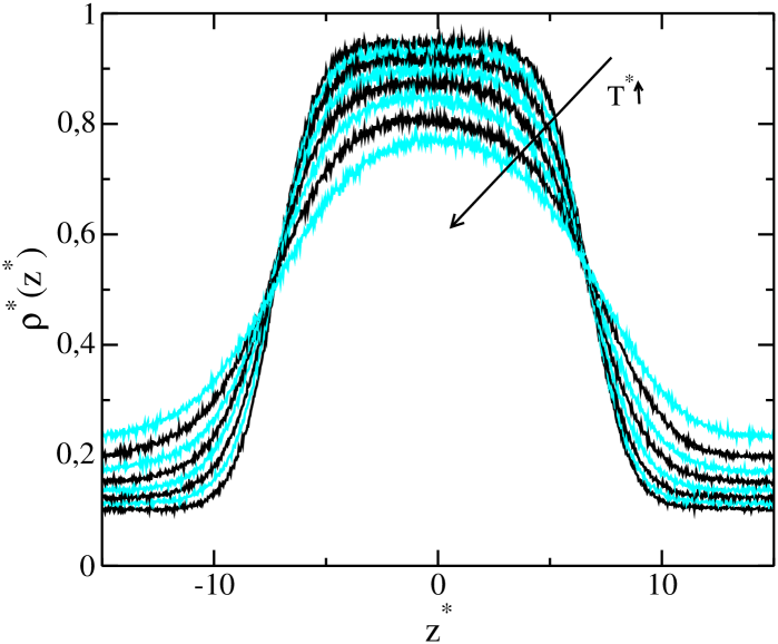
Figure 2: Density profiles along the largest cell side (normal to the interfaces) for the shortest range case, $s=0.2$. Different curves correspond to different temperatures. The arrow points to the direction of increasing temperature.

The trajectories are then analyzed by means of a simple home made program code which produces the density profiles (fixing the system center of mass at the parallelepiped geometrical center) and discards the first steps where energy has not reached a clear plateau. The output is shown in figure 2 for $s=0.2$ and for all different temperatures. It is worth mentioning that the difficulty for getting acceptable profiles increases with decreasing the potential range. As can be seen in figure 1 the potential shape is quite sharp for $s=0.2$. Such a short range implies low coexistence temperatures, long living bonds, a slow dynamics, and a more likely crystallization. Hence, we are showing the most difficult case. The profiles are then employed to obtain the vapor and liquid densities from the fully developed bulk regions. Note that there is not a clear liquid bulk region for the largest temperature shown in figure 2. In such a case the point is discarded for determining the critical properties. The critical density $\rho^{*}_{c}$ and temperature $T^{*}_{c}$ are obtained by considering the effective critical exponent $\beta_{e}=0.325$ and from the law of rectilinear diameters. The critical pressure is taken from a linear extrapolation of the logarithm of the vapor pressure against the reciprocal temperature towards $1/T^{*}_{c}$.

The pressure tensor is obtained from the virial expression Frenkel and Smit (1996). In turn, the surface tension can be found by means of

$$\gamma=\frac{L_{z}}{2}\left\{\langle P_{zz}\rangle-1/2(\langle P_{xx}\rangle+\langle P_{yy}\rangle)\right\}$$ (2)

where $P_{ii}$ ($i=$ $x$, $y$, $z$) are the diagonal components. The factor 2 is due to the existence of two interfaces. Our output is identical to the one obtained from the Gromacs tools (g_energy) once the factor of 2 is accounted for. The vapor pressure, $P$, is taken as the normal to the interfaces, $P_{zz}$.

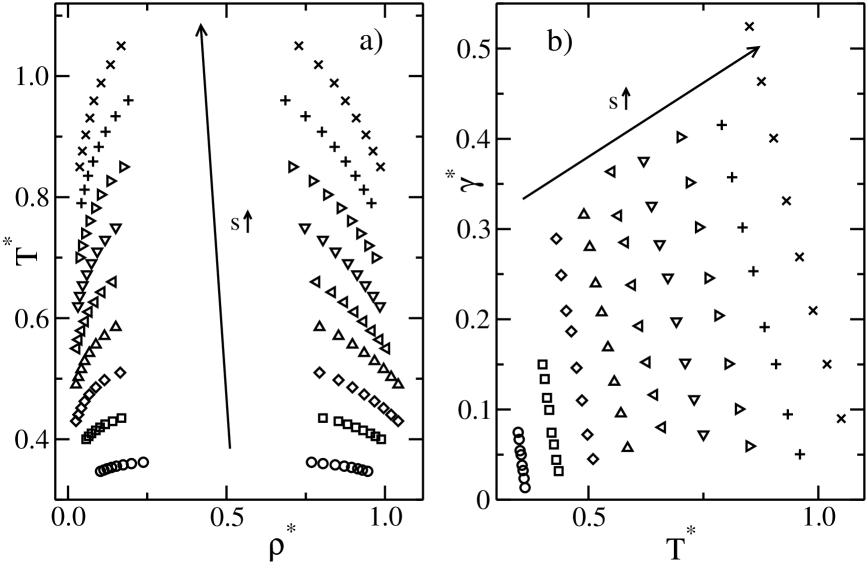
Figure 3: a) Vapor-liquid coexistence density curves for the ANC potential with varying $s$. Circles, squares, diamonds, triangles-up, triangles-left, triangles-down, triangles-right, plus symbols, and crosses correspond to $s=0.2,0.3,0.4,0.5,0.6,0.7,0.8,0.9,$ and $1.0$, respectively. b) The corresponding dimensionless surface tension (the estimated error is always below $5\%$). Arrows indicate the direction of increasing $s$.

In previous work we have defined $B_{2s}^{*}(T^{*})=B_{2}^{*}(T^{*})-B_{2}^{*}(T^{*}_{c})+cst.$ where $B_{2}^{*}(T^{*})=3B_{2}(T^{*})/(2\pi\sigma^{*3}_{eff}(T^{*}))$,

$$B_{2}(T^{*})=2\pi\int_{0}^{\infty}r^{*2}[1-e^{-u^{*}(r^{*})/T^{*}}]dr^{*},$$ (3)

$$\sigma^{*}_{eff}(T^{*})=\int_{0}^{\infty}[1-e^{-u^{\prime*}(r^{*})/T^{*}}]dr^{*},$$ (4)

$u^{\prime*}(r^{*})=u^{*}(r^{*})+1$ for $r^{*}<1$ and $u^{\prime}(r^{*})=0$ otherwise Andersen et al. (1971); Barker and Henderson (1976). Note that $2\pi\sigma^{*3}_{eff}(T^{*})/3$ is the second virial coefficient of hard spheres with a hard core diameter of $\sigma^{*}_{eff}$. There, we have employed $cst.=-1.5$ to gain consistency with previous works. Now we are setting $cst.=0$ to gain simplicity of the expressions. Furthermore, the difference between the reduced second virial coefficient at $T^{*}$ and $T^{*}_{c}$ would be our measure of the attractive range. This way, the fitted expressions for the liquid and vapor branches of the coexistence are given by

$$B^{*}_{2s}(\rho^{*})=-0.475(\rho^{*}-1)^{3.1}$$ (5)

and

$$B^{*}_{2s}(\rho^{*})=-(b\rho^{*3}+c\rho^{*1/2})^{-1}+(b+c)^{-1}$$ (6)

with $b=75.1$ and $c=3.71$, respectively. These expressions were obtained by means of a trial and error procedure and correspond to both, the Mie and Yukawa potentials.

III Results

As explained, from the fully developed liquid and vapor bulk phases we obtain coexistence densities. These are presented in figure 3 a). There are eight points per curve, each one corresponding to a different value of the softness parameter, $s$. Each of the eight points corresponding, in turn, to different temperatures (we are setting eight replicas). The embedded arrow in the left panel shows the increasing $s$ direction. Curves shift to larger temperatures when increasing the potential range, as usual (more kinetic energy is required to produce the vapor phase). Note also that the temperature window is strongly reduced for the strong short range cases. This is done on purpose to avoid the formation of a crystal phase (a short range potential combined with a monodisperse central-core enhance crystallization). Also, the small temperatures lead to long lived bonds which yield a slow system dynamics. Both issues make it difficult to obtain coexistence vapor-liquid curves for strong short range interactions. The data are in good agreement with the Gibbs ensemble Monte Carlo simulations reported in reference del Río et al. (2007). The $s$ range in their study is $0.6\leq s\leq 1.2$. For $s=0.5$ our data are in good agreement with those reported in reference del Río et al. (2005). To the best of our knowledge, there are no vapor-liquid coexistence data reported in the literature for $s<0.5$.

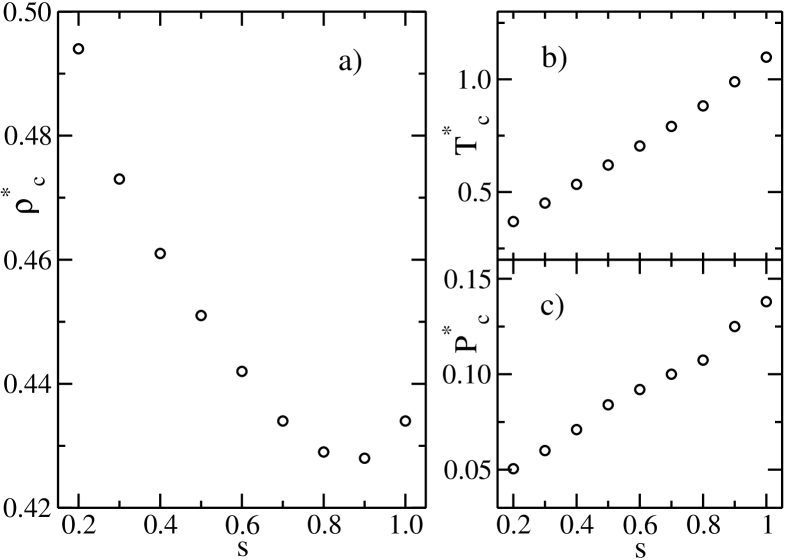
Figure 4: Critical properties as a function of $s$. a) Dimensionless critical density, b) temperature, and c) vapor pressure. Estimated errors for density, temperature, and vapor pressure are always below $4\%$, $2\%$, and $4\%$, respectively. Numerical values are given in table 1.

Table 1: Dimensionless critical properties of the ANC potential as a function of its softness, $s$. Estimated errors are always lower than 2$\%$, 4$\%$, and 4$\%$, for $T^{*}$, $\rho_{c}^{*}$, and $P_{c}^{*}$, respectively. $Z_{c}$ is obtained from $P_{c}^{*}/(T_{c}^{*}\rho_{c}^{*})$ and thus its error is lower than $10\%$.

$s$	$T_{c}^{*}$	$\rho_{c}^{*}$	$P_{c}^{*}$	$Z_{c}$	$B^{*}_{2}(T_{c}^{*})$
0.20	0.369	0.494	0.051	0.277	-1.309
0.30	0.451	0.473	0.060	0.281	-1.331
0.40	0.534	0.461	0.071	0.288	-1.362
0.50	0.620	0.451	0.084	0.300	-1.387
0.60	0.704	0.442	0.092	0.296	-1.438
0.70	0.791	0.434	0.100	0.291	-1.490
0.80	0.882	0.429	0.107	0.284	-1.541
0.90	0.989	0.428	0.125	0.295	-1.559
1.00	1.098	0.434	0.138	0.290	-1.597

Dimensionless surface tension data are shown in figure 3 b). Different symbols are used for different values of $s$, in correspondence with panel a). The arrow points along the increasing $s$ direction. As expected, the values increase with decreasing temperature and tend to zero as approaching the critical temperature. Also, curves shift to the right with increasing $s$, in correspondence to the vapor-liquid coexistence densities. Data for $s=0.5$ agree well with those given in reference del Río et al. (2005). For $s>0.5$ our data are well above theirs, most probably due to the use of an insufficiently large cutoff, as the authors explain in reference del Río et al. (2007). Indeed, the differences between our data and those reported in reference del Río et al. (2005) increase with increasing $s$ confirming this claim. Hence, our surface tension data for $s>0.5$ can be considered as the first clean ones given in the literature. In addition, the surface tension for the region $0.2\leq s\leq 0.4$ is technically difficult to access. Hence, and as for the coexistence, there are no previously reported surface tension data for this region.

The monotonic and practically linear trend of the critical temperature with $s$ is shown in figure 4 b). Values agree with previously reported data del Río et al. (2007) in the interval $0.6\leq s\leq 1.0$. Also, the critical vapor pressure shows a linear behavior with $s$, figure 4 c). Here the general trend agrees with the trend observed by del Río et. al del Río et al. (2007). Our values are, however, somewhat smaller than theirs. As expected, both properties increase with the potential range. Conversely, the critical density shows a more complex behavior, as it is shown in the main panel of figure 4. It probably shows a minimum close to $s=0.9$, or simply shift from a clear decay for $s\leq 0.6$ to a plateau at the interval $0.8\leq s\leq 1.0$. The uncertainty of the data does not allow us to discern one scenario from the other. Nonetheless, our data show a better defined trend than those reported elsewhere del Río et al. (2005, 2007). We get a plateau for the critical compressibility, $Z^{*}_{c}=P^{*}_{c}/(T^{*}_{c}\rho_{c})$, for $s>0.4$ and a probable slight decrease for $s<0.4$ (see table 1). Again, the uncertainty of the data hinders the trend which seems to be in line with the one reported in ref. del Río et al. (2007). Finally, the reduced second virial coefficient at the critical temperature $B_{2}^{*}(T^{*}_{c})$ is an ever decreasing function of $s$ in the studied interval. It decays from $-1.309$ to $-1.597$ (see table 1).

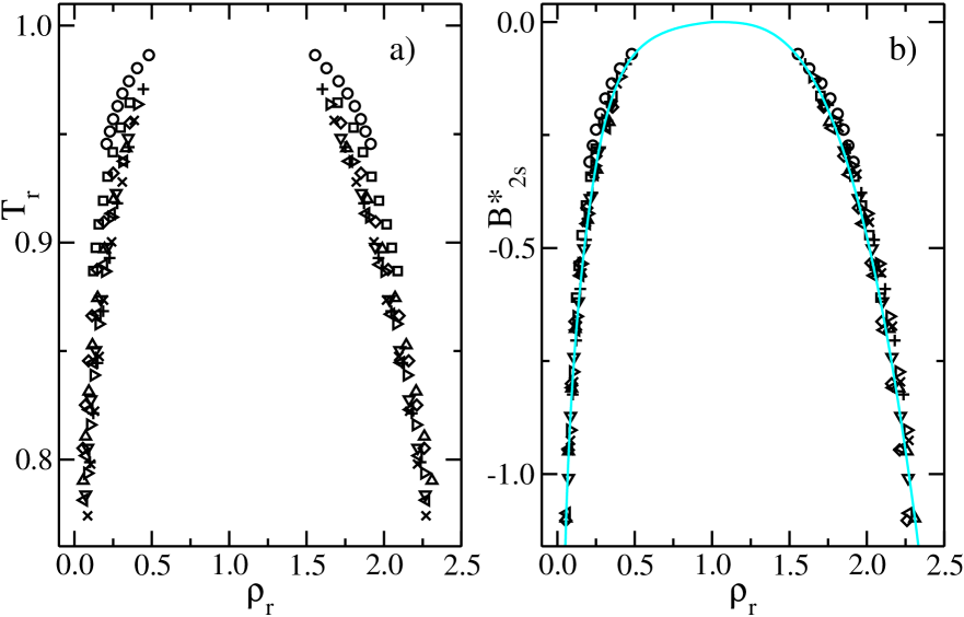
Figure 5: Vapor-liquid coexistence for the ANC potential with varying $s$. Different symbols are employed for different $s$ values, in correspondence with figure 3. a) $T_{r}-\rho_{r}$ chart as following the van der Waals principle. b) $B_{2s}^{*}-\rho_{r}$ chart. This last chart includes the master curve fit to the Mie and Yukawa potential as a light (cyan) line (equations 5 and 6).

Up to this point, we have shown raw data obtained for some vapor-liquid coexistence and surface properties for the ANC potential by varying $s$ (see table 2). From here on, we are comparing the outputs from the van der Waals principle to those of the extended framework with $B^{*}_{2s}$. We are omitting plots against $B^{*}_{2}$ due to the $B^{*}_{2}(T^{*}_{c})$ dependence on $s$. Figure 5 shows the results of applying the van der Waals (left panel) and extended (right panel) frameworks to the vapor-liquid coexistence. Reduced properties are given by $T_{r}=T^{*}/T^{*}_{c}$ and $\rho_{r}=\rho^{*}/\rho^{*}_{c}$. It is observed how the relatively good data collapse on the left panel is improved on the right one. This was already pointed out for the Mie and Yukawa potentials Orea et al. (2015). Moreover, we are including the master curve obtained from these potentials as a light (cyan) line which, as can be seen, can be considered a fit to these new data. So, Mie, Yukawa, and ANC lead to the same coexistence density master curve, which imply a correspondence between their attractive ranges irrespective of their different shape. This result is encouraging since, letting aside the square-well potential case Orea et al. (2015), expressions 5 and 6 seem general. Nonetheless, further testing is needed.

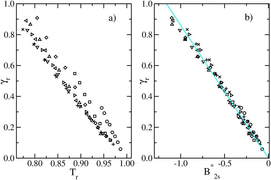
Figure 6: Surface tension for the ANC potential with varying $s$. Different symbols are employed for different $s$ values, in correspondence with figure 3. a) $\gamma_{r}-T_{r}$ chart as following the van der Waals principle. b) $\gamma_{r}-B_{2s}^{*}$ chart. The linear fit $\gamma_{r}=-0.86B^{*}_{2s}$ is shown as a light (cyan) line.

We now focus our attention on how the corresponding states frameworks behave when dealing with properties such as the surface tension and vapor pressure. The left panel of figure 6 shows a $\gamma_{r}-T_{r}$ chart with $\gamma_{r}=\gamma^{*}/(\rho^{*}_{c}T_{c}^{*2/3})$. Likewise, figure 6 b) shows $\gamma_{r}$ as a function of $B^{*}_{2s}$. Again, there is a gain of the data collapse when employing $B^{*}_{2s}$ instead of $T_{r}$ as the independent variable. In the left panel, circles, squares, and probably diamonds, are far from where the other points concentrate. This series corresponds to $s=0.2$, 0.3, and 0.4, respectively. So, the scattering of the curves increases with decreasing $s$. We may say that the collapse appears only for $s>0.4$ under the van der Waals framework. This situation is not observed in the right-side panel, where all curves seem to obey the corresponding states principle. In addition, in base of the estimated errors, we cannot discard a linear behavior for the general shape of the obtained master curve. This line has a slope of $-0.86$ and zero $y$-intercept.

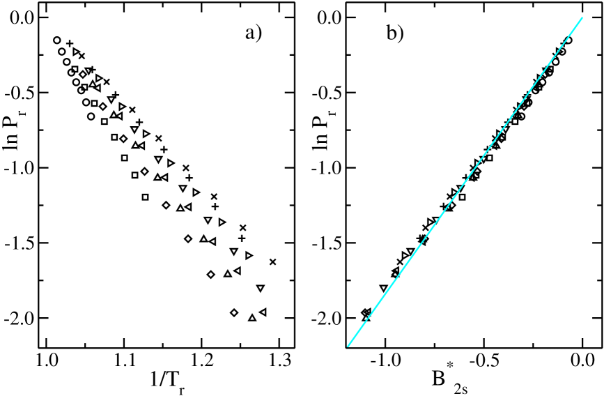
Figure 7: Logarithm of the vapor pressure for the ANC potential with varying $s$. Different symbols are employed for different $s$ values, in correspondence with figure 3. a) As a function of $1/T_{r}$ as following the van der Waals principle. b) As a function of $B_{2s}^{*}$. The linear fit $\ln P_{r}=1.84B^{*}_{2s}$ is shown as a light (cyan) line.

Finally, we show the logarithm of the reduced vapor pressure, ln $P_{r}=$ ln $(P^{*}/P^{*}_{c})$, as a function of $1/T_{r}$ in figure 7 a) and as a function of $B^{*}_{2s}$ in figure 7 b). Well defined straight lines are defined in the left panel. Their slopes (absolute value), however, decrease monotonically with increasing $s$ for all the studied interval. So, a master curve cannot be defined. This picture changes when considering the extended framework where a single curve appears. Furthermore, the curve turns linear when directly plotted against $B^{*}_{2s}$. The fitted expression, shown as a light line, reads $\ln P_{r}=1.84B^{*}_{2s}$. All data lie on this curve when taking into account their corresponding error bars (not shown to gain clarity).

IV Conclusions

We have reported the vapor-liquid coexistence density, vapor pressure, and surface tension for the ANC potential (expression 1) of variable range. Its softness parameter, $s$, has been set in the range $0.2\leq s\leq 1.0$ at intervals of $0.1$. This was done by means of molecular dynamics simulations (Gromacs package) in the $NVT$ ensemble. For this purpose, a rectangular parallelepiped cell was employed having a liquid slab and two vapor-liquid interfaces. Our data agree well with previously reported data for the coexisting vapor-liquid densities in the interval $0.5\leq s\leq 1.0$ and for the surface tension with $s=0.5$. All properties in the interval $0.2\leq s\leq 0.4$ are reported for the first time. These short range cases are technically difficult to access with simulations. We have found a linear relationship between $T_{c}$, $P_{c}$ and $s$. Conversely, $\rho_{c}$ is not a linear function of $s$. These trends were not clear from previous results.

The van der Waals and extended law frameworks were applied to the obtained data. This was carried out for vapor-liquid coexistence densities, surface tension, and vapor pressure. For all cases, a much better data collapse is observed when using $B^{*}_{2s}$ as an independent variable instead of the reduced temperature. Furthermore, the obtained coexistence density master curve is practically the same we have found for the Mie and the Yukawa potentials. Finally, the master curves found for surface tension and vapor pressure are strikingly simple and tentatively universal. In view of the presented results, we expect the master curves for these properties to hold for the Mie and Yukawa potential. We also expect other spherically symmetric pair potentials to behave in line with the ANC, Mie, and Yukawa fluids. This would imply a correspondence between their attractive ranges irrespective of their different shape.

V Acknowledgments

PO and AR thank the Instituto Mexicano del Petróleo for financial support (Project No D.61017). PO also thanks the IMP Project No Y.60013. GO thanks CONACyT Project No 169125.

Table 2: Phase coexistence and interfacial properties as a function of temperature for the ANC potential with different softness ($s$). All properties are dimensionless.

$s$	$T^{*}$	$\rho_{L}^{*}$	$\rho_{V}^{*}$	$P^{*}$	$\gamma^{*}$	$B_{2}^{*}$
0.2	0.3470	0.9456	0.1027	0.0246	0.0747	-1.6186
	0.3491	0.9288	0.1133	0.0270	0.0669	-1.5825
	0.3512	0.9141	0.1237	0.0292	0.0544	-1.5471
	0.3534	0.8948	0.1376	0.0309	0.0498	-1.5124
	0.3555	0.8715	0.1530	0.0329	0.0383	-1.4783
	0.3576	0.8429	0.1740	0.0353	0.0324	-1.4449
	0.3598	0.8044	0.2001	0.0378	0.0236	-1.4121
	0.3620	0.7683	0.2376	0.0408	0.0134	-1.3799
0.3	0.4000	0.9880	0.0573	0.0182	0.1499	-1.9408
	0.4048	0.9699	0.0653	0.0210	0.1338	-1.8705
	0.4097	0.9539	0.0742	0.0236	0.1129	-1.8025
	0.4146	0.9308	0.0877	0.0271	0.0995	-1.7368
	0.4196	0.9079	0.1012	0.0300	0.0743	-1.6732
	0.4247	0.8817	0.1173	0.0339	0.0613	-1.6116
	0.4298	0.8531	0.1407	0.0378	0.0442	-1.5520
	0.4350	0.8043	0.1687	0.0426	0.0317	-1.4943
0.4	0.4300	1.0417	0.0253	0.0099	0.2893	-2.4651
	0.4406	1.0195	0.0327	0.0128	0.2489	-2.3089
	0.4515	0.9956	0.0418	0.0162	0.2093	-2.1624
	0.4626	0.9669	0.0523	0.0202	0.1866	-2.0248
	0.4740	0.9344	0.0674	0.0253	0.1462	-1.8954
	0.4857	0.8971	0.0879	0.0315	0.1101	-1.7736
	0.4977	0.8535	0.1152	0.0390	0.0722	-1.6588
	0.5100	0.7934	0.1648	0.0483	0.0451	-1.5504
0.5	0.4900	1.0417	0.0253	0.0113	0.3157	-2.4847
	0.5026	1.0195	0.0327	0.0152	0.2800	-2.3366
	0.5154	0.9956	0.0418	0.0192	0.2395	-2.1971
	0.5287	0.9669	0.0523	0.0235	0.2075	-2.0655
	0.5422	0.9344	0.0674	0.0289	0.1686	-1.9413
	0.5561	0.8971	0.0879	0.0357	0.1306	-1.8239
	0.5704	0.8535	0.1152	0.0437	0.0955	-1.7129
	0.5850	0.7934	0.1508	0.0537	0.0572	-1.6078

$s$	$T^{*}$	$\rho_{L}^{*}$	$\rho_{V}^{*}$	$P^{*}$	$\gamma^{*}$	$B_{2}^{*}$
0.6	0.5500	1.0040	0.0267	0.0129	0.3636	-2.5252
	0.5645	0.9830	0.0334	0.0170	0.3148	-2.3826
	0.5794	0.9583	0.0423	0.0207	0.2852	-2.2477
	0.5947	0.9321	0.0537	0.0261	0.2380	-2.1201
	0.6104	0.9038	0.0655	0.0317	0.1926	-1.9993
	0.6265	0.8713	0.0842	0.0392	0.1524	-1.8848
	0.6430	0.8329	0.1061	0.0477	0.1163	-1.7762
	0.6600	0.7839	0.1412	0.0575	0.0803	-1.6730
0.7	0.6200	0.9840	0.0316	0.0166	0.3758	-2.4991
	0.6371	0.9627	0.0373	0.0212	0.3260	-2.3617
	0.6547	0.9382	0.0464	0.0261	0.2834	-2.2316
	0.6727	0.9123	0.0595	0.0323	0.2464	-2.1082
	0.6912	0.8831	0.0740	0.0391	0.1978	-1.9911
	0.7103	0.8438	0.0923	0.0477	0.1521	-1.8798
	0.7299	0.8043	0.1170	0.0582	0.1117	-1.7741
	0.7500	0.7472	0.1508	0.0706	0.0725	-1.6734
0.8	0.7000	0.9702	0.0357	0.0220	0.4019	-2.4442
	0.7197	0.9466	0.0437	0.0275	0.3515	-2.3153
	0.7399	0.9215	0.0536	0.0335	0.3020	-2.1928
	0.7607	0.8923	0.0672	0.0407	0.2457	-2.0763
	0.7821	0.8596	0.0850	0.0495	0.2041	-1.9653
	0.8041	0.8171	0.1033	0.0594	0.1506	-1.8597
	0.8267	0.7717	0.1331	0.0717	0.1005	-1.7589
	0.8500	0.7075	0.1740	0.0855	0.0594	-1.6628
0.9	0.7900	0.9573	0.0425	0.0287	0.4153	-2.3831
	0.8123	0.9331	0.0522	0.0355	0.3574	-2.2636
	0.8352	0.9069	0.0634	0.0430	0.3017	-2.1496
	0.8588	0.8762	0.0791	0.0519	0.2532	-2.0408
	0.8831	0.8411	0.0971	0.0622	0.1913	-1.9369
	0.9080	0.8010	0.1185	0.0747	0.1502	-1.8376
	0.9336	0.7491	0.1500	0.0883	0.0946	-1.7427
	0.9600	0.6857	0.1904	0.1051	0.0504	-1.6518

$s$	$T^{*}$	$\rho_{L}^{*}$	$\rho_{V}^{*}$	$P^{*}$	$\gamma^{*}$	$B_{2}^{*}$
1.0	0.8500	0.9859	0.0370	0.0271	0.5245	-2.5230
	0.8761	0.9622	0.0454	0.0340	0.4635	-2.3935
	0.9029	0.9399	0.0561	0.0418	0.4007	-2.2701
	0.9306	0.9092	0.0691	0.0506	0.3313	-2.1526
	0.9591	0.8751	0.0815	0.0616	0.2691	-2.0405
	0.9885	0.8399	0.1043	0.0745	0.2097	-1.9336
	1.0188	0.7902	0.1340	0.0896	0.1502	-1.8315
	1.0500	0.7283	0.1677	0.1065	0.0899	-1.7340

References

- Pitzer (1939) K. E. Pitzer, J. Chem. Phys. 7, 583 (1939).
- Okumura and Yonezawa (2000) H. Okumura and F. Yonezawa, J. Chem. Phys. 113, 9162 (2000).
- Dunikov et al. (2001) D. O. Dunikov, S. P. Malyshenko, and V. V. Zhakhovskii, J. Chem. Phys. 115, 6623 (2001).
- Orea et al. (2008) P. Orea, Y. Reyes-Mercado, and Y. Duda, Phys. Lett. A 372, 7024 (2008).
- Galliero et al. (2009) G. Galliero, M. M. Piñeiro, B. Mendiboure, C. Miqueu, T. Lafitte, and D. Bessieres, J. Chem. Phys. 130, 104704 (2009).
- Blas et al. (2012a) F. J. Blas, F. J. Martínez-Ruiz, A. I. Moreno-Ventas Bravo, and L. G. MacDowell, J. Chem. Phys. 137, 024702 (2012a).
- Blas et al. (2012b) F. J. Blas, A. I. Moreno-Ventas Bravo, J. M. Míguez, M. M. Piñeiro, and L. G. MacDowell, J. Chem. Phys. 137, 084706 (2012b).
- Chapela et al. (2013) G. A. Chapela, E. Díaz-Herrera, J. C. Armas-Pérez, and J. Quintana-H, J. Chem. Phys. 138, 224509 (2013).
- Martínez-Valencia et al. (2013) A. Martínez-Valencia, M. González-Melchor, P. Orea, and J. López-Lemus, Mol. Sim. 39, 64 (2013).
- Patra et al. (2012) T. K. Patra, A. Hens, and J. K. Singh, J. Chem. Phys. 137, 084701 (2012).
- Katsonis et al. (2006) P. Katsonis, S. Brandon, and P. G. Vekilov, J. Phys. Chem. B 110, 17638 (2006).
- Valadez-Pérez et al. (2012) N. E. Valadez-Pérez, A. L. Benavides, E. Schöll-Paschinger, and R. Castañeda Priego, J. Chem. Phys. 137, 084905 (2012).
- Román et al. (2005) F. Román, J. White, S. Velasco, and A. Mulero, J. Chem. Phys. 123, 124512 (2005).
- Weiss and Schröer (2007) V. C. Weiss and W. Schröer, Int. J. Thermophys. 28, 506 (2007).
- Galliero (2010) G. Galliero, J. Chem. Phys. 133, 074705 (2010).
- Wei et al. (2013) L. M. Wei, P. Li, L. W. Qiao, and K. T. Tang, J. Chem. Phys. 139, 154306 (2013).
- Mousazadeh et al. (2006) M. Mousazadeh, A. Khanchi, and G. Marageh, J. Iranian Chem. Soc. 3, 22 (2006).
- Castellanos et al. (2004) A. Castellanos, G. Urbina-Villalba, and M. García-Sucre, J. Phys. Chem. B 108, 5951 (2004).
- Ghatee et al. (2002) M. H. Ghatee, A. Maleki, and H. Ghaed-Sharaf, Langmuir 19, 211 (2002).
- Puosi and Leporini (2011) F. Puosi and D. Leporini, J. Phys. Chem. B 115, 14046 (2011).
- Boire et al. (2013) A. Boire, P. Menut, M. H. Morel, and C. Sanchez, Soft Matter 9, 11417 (2013).
- Ubbelohde (1965) A. R. Ubbelohde, Melting and Crystal Structure (Clarendon: Oxford, 1965).
- Rosenfeld (1977) Y. Rosenfeld, Phys. Rev. A 15, 2545 (1977).
- Young and Andersen (2003) T. Young and C. Andersen, H, J. Chem. Phys. 118, 3447 (2003).
- Galliero et al. (2007) G. Galliero, C. Boned, A. Baylaucq, and F. Montel, Chem. Phys. 333, 219–228 (2007).
- Galliero and Boned (2008) G. Galliero and C. Boned, J. Chem. Phys. 129, 074506 (2008).
- Bacher et al. (2014) A. K. Bacher, T. B. Schrøder, and J. C. Dyre, Nature Comm. 5, 5424 (2014).
- Dyre (2014) J. C. Dyre, J. Phys. Chem. B 118, 10007 (2014).
- Noro and Frenkel (2000) M. G. Noro and D. Frenkel, J. Chem. Phys. 113, 2941 (2000).
- Orea et al. (2015) P. Orea, S. Varga, and G. Odriozola, Chem. Phys. Lett. 631–632, 26 (2015).
- Guggenheim (1945) E. A. Guggenheim, J. Chem. Phys. 13, 253 (1945).
- Hunter (2001) R. J. Hunter, Foundations of Colloid Science (Oxford University Press, Oxford, 2001).
- Vliegenthart and Lekkerkerker (2000) G. A. Vliegenthart and H. N. W. Lekkerkerker, J. Chem. Phys. 112, 5364 (2000).
- del Río et al. (2005) F. del Río, E. Díaz-Herrera, E. Ávalos, and J. Alejandre, J. Chem. Phys. 122, 034504 (2005).
- Kihara (1954) T. Kihara, J. Phys. Soc. Japan 6, 289 (1954).
- McLure et al. (1999) I. A. McLure, J. E. Ramos, and F. del Río, J. Phys. Chem. B 103, 7019 (1999).
- del Río et al. (2007) F. del Río, O. Guzmán, J. E. Ramos, and B. Ibarra-Tandi, Fluid Phase Equilib. 259, 9 (2007).
- del Río et al. (2013) F. del Río, E. Díaz-Herrera, O. Guzmán, J. A. Moreno-Razo, and J. E. Ramos, J. Chem. Phys. 139, 184503 (2013).
- González-Calderón and Rocha-Ichante (2015) A. González-Calderón and A. Rocha-Ichante, J. Chem. Phys. 142, 034305 (2015).
- van der Spoel et al. (2005) D. van der Spoel, E. Lindahl, B. Hess, G. Groenhof, A. E. Mark, and H. J. C. Berendsen, J. Comp. Chem. 26, 1701 (2005).
- Hess et al. (2008) B. Hess, C. Kutzner, D. van der Spoel, and E. Lindahl, J. Chem. Theory Comp. 4, 435 (2008).
- del Río et al. (1998) F. del Río, J. E. Ramos, and I. A. McLure, J. Phys. Chem. B 102, 10568 (1998).
- Lyubartsev et al. (1992) A. P. Lyubartsev, A. A. Martsinovski, S. V. Shevkunov, and P. N. Vorontsov-Velyaminov, J. Chem. Phys. 96, 1776 (1992).
- Marinari and Parisi (1992) E. Marinari and G. Parisi, Europhys. Lett. 19, 451 (1992).
- Bussi et al. (2007) G. Bussi, D. Donadio, and M. Parrinello, J. Chem. Phys. 126, 014101 (2007).
- Chapela et al. (1977) G. A. Chapela, G. Saville, S. M. Thompson, and J. S. Rowlinson, J. Chem. Soc. Faraday Trans. II 73, 1133 (1977).
- Frenkel and Smit (1996) D. Frenkel and B. Smit, Understanding molecular simulation (Academic, New York, 1996).
- Andersen et al. (1971) H. C. Andersen, J. D. Weeks, and D. Chandler, Phys. Rev. A 4, 1597 (1971).
- Barker and Henderson (1976) J. A. Barker and D. Henderson, Rev. Mod. Phys. 48, 587 (1976).