Evolution equation for the higher-twist B-meson distribution amplitudes

Abstract

We find that the evolution equation for the three-particle quark-gluon B-meson light-cone distribution amplitude (DA) of subleading twist is completely integrable in the large $N_{c}$ limit and can be solved exactly. The lowest anomalous dimension is separated from the rest, continuous, spectrum by a finite gap. The corresponding eigenfunction coincides with the contribution of quark-gluon states to the two-particle DA $\phi_{-}(\omega)$ so that the evolution equation for the latter is the same as for the leading-twist DA $\phi_{+}(\omega)$ up to a constant shift in the anomalous dimension. Thus “genuine” three-particle states that belong to the continuous spectrum effectively decouple from $\phi_{-}(\omega)$ to the leading-order accuracy. In turn, the scale dependence of the full three-particle DA turns out to be nontrivial so that the contribution with the lowest anomalous dimension does not become leading at any scales. The results are illustrated on a simple model that can be used in studies of $1/m_{b}$ corrections to heavy-meson decays in the framework of QCD factorization or light-cone sum rules.

I Introduction

B-meson light-cone distribution amplitudes (DAs) are the main nonperturbative input to the QCD description of weak decays involving light hadrons in the final state Beneke:1999br ; Beneke:2000wa . In particular the leading-twist DA gives a dominant contribution in the heavy quark expansion and it received considerable attention already Grozin:1996pq ; Lange:2003ff ; Braun:2003wx ; Lee:2005gza ; Bell:2013tfa ; Braun:2014owa ; Feldmann:2014ika . Utility of the QCD factorization techniques depends, however, on the possibility to control, or at least estimate, the corrections suppressed by powers of the $b$-quark mass that involve higher-twist DAs. This task is attracting increasing attention and in the last years there have been several efforts to combine light-cone sum rules with the expansion in terms of B-meson DAs Khodjamirian:2006st ; DeFazio:2007hw ; Braun:2012kp ; Wang:2015vgv . This technique allows one to tame infrared divergences which appear power-suppressed contributions in the purely perturbative framework and to calculate the so-called soft or end-point nonfactorizable contributions in terms of the DAs of increasing twist. One of the problems on this way is that higher-twist B-meson DAs involve contributions of multiparton states and are practically unknown.

In this letter we point out that the structure of subleading twist DAs is simpler as compared to what one may assume from their general partonic decomposition Kawamura:2001jm ; Nishikawa:2011qk . This structure is revealed by considering the scale dependence of the DAs in the limit of large number of colors, $N_{c}\to\infty$, i.e. neglecting the $1/N_{c}^{2}$ corrections to the renormalization group equations. It turns out that the evolution equation for the three-particle DA in this approximation is completely integrable and can be solved exactly. The lowest anomalous dimension is separated from the rest, continuous, spectrum by a finite gap. The corresponding eigenfunction defines what can be called the “asymptotic” three-particle B-meson DA and has a relatively simple form. Most remarkably, it turns out that the higher-twist contribution to the two-particle B-meson DA $\phi_{-}(\omega)$ that is related to the three-particle DA by QCD equations of motion (EOM), is expressed entirely in terms of this “asymptotic” state, the states that belong to the continuous spectrum do not contribute. As the result the DA $\phi_{-}(\omega)$ evolves autonomously and does not mix with “genuine” three-particle contributions. The evolution equation for $\phi_{-}(\omega)$ is the same as for the leading-twist DA $\phi_{+}(\omega)$ up to a constant shift in the anomalous dimension. Finally, we discuss the evolution of the three-particle DA itself and its asymptotic behavior at small and large quark/gluon momenta which turns out to be nontrivial. This behavior is illustrated on the example of a simple model that can be used in phenomenological applications.

II Evolution equations

Following the established conventions Grozin:1996pq we define the B-meson DAs as matrix elements of the renormalized nonlocal operators built of an effective heavy quark field $h_{v}(0)$, a light (anti)quark and gluons at a light-like separation:

$$iF(\mu)\Phi_{+}(z,\mu) =\langle 0|\bar{q}(nz)\not{n}\gamma_{5}h_{v}(0)|\bar{B}(v)\rangle,$$

$$iF(\mu)\Phi_{-}(z,\mu) =\langle 0|\bar{q}(nz)\not{\bar{n}}\gamma_{5}h_{v}(0)|\bar{B}(v)\rangle$$ (1)

and

$$-2iF(\mu)\Phi_{3}(z_{1},z_{2},\mu)=$$ (2)

$$= \langle 0|\bar{q}(nz_{1})gG_{\mu\nu}(nz_{2})n^{\nu}\sigma^{\mu\rho}n_{\rho}\gamma_{5}h_{v}(0)|\bar{B}(v)\rangle.$$

Here $v_{\mu}$ is the heavy quark velocity, $n_{\mu}$ is the light-like vector, $n^{2}=0$, such that $n\cdot v=1$, $\Gamma$ stands for an arbitrary Dirac structure, $|\bar{B}(v)\rangle$ is the $\bar{B}$-meson state, $\mu$ is the factorization scale and $F(\mu)$ is the B-meson decay constant in the heavy quark effective theory (HQET). Wilson lines connecting the fields are not shown for brevity; they are always implied.

The functions $\Phi_{+}$ and $\Phi_{-}$ are the leading- and subleading-twist two-particle B-meson DAs Beneke:2000wa , and $\Phi_{3}$ is the (lowest twist) three-particle DA that is the only one relevant for the present study. In notations of Kawamura:2001jm $\Phi_{3}={\Psi}_{A}-{\Psi}_{V}$. These three DAs are related by an EOM Beneke:2000wa ; Kawamura:2001jm

$$(1+z\partial_{z})\,\Phi_{-}(z)=\Phi_{+}(z)+2\int_{0}^{z}\!wdw\,\Phi_{3}(z,w)\,$$ (3)

that can be solved to obtain $\Phi_{-}$ as a sum of the so-called Wandzura-Wilczek (WW) term expressed in terms of $\Phi_{+}$ Beneke:2000wa , and a certain integral of the quark-gluon DA $\Phi_{3}$. The latter contribution is nontrivial because it involves a function of two variables. We will demonstrate, however, that this complication is to a large extent illusory as the integral appearing in the EOM essentially decouples from “genuine” quark-gluon correlations. This simplification is exactly analogous to what has been observed before Ali:1991em ; Balitsky:1996uh ; Braun:2000av ; Braun:2001qx for the structure function $g_{2}(x,Q^{2})$ in polarized deep-inelastic lepton-proton scattering.

The following discussion is based on properties of the renormalization group equations for heavy-light operators under collinear conformal transformations. The corresponding generators read

$$S_{+}=z^{2}\partial_{z}+2jz\,, S_{0}=z\partial_{z}+j\,, S_{-}=-\partial_{z}\,,$$ (4)

where $j$ is the conformal spin, $j_{q}=1$ for the light quark and $j_{g}=3/2$ for the gluon. The generators satisfy the standard $SL(2)$ commutation relations $[S_{+},S_{-}]=2S_{0}\,,\quad[S_{0},S_{\pm}]=\pm S_{\pm}\,.$ We distinguish the generators acting on quark and gluon coordinates by the subscript $S_{q}$ and $S_{g}$, respectively.

The starting observation is that both the one-loop renormalization group equations (RGE) for the DAs and the EOM relations are invariant under special conformal transformations Knodlseder:2011gc ; Braun:2014owa . It is therefore natural to expand the DAs in terms of the eigenfunctions of the corresponding generator Braun:2014owa

$$Q_{s}^{(j)}(z)=\frac{e^{-i\pi j}}{z^{2j}}e^{is/z}\,, iS^{(j)}_{+}Q_{s}^{(j)}=sQ_{s}^{(j)}\,.$$ (5)

They form a complete orthonormal set

$$\langle{Q_{s}^{(j)}|Q_{s^{\prime}}^{(j)}\rangle}_{j}={\Gamma(2j)}{s^{1-2j}}\,\delta(s-s^{\prime})\,,$$ (6)

$$\frac{1}{\Gamma(2j)}\int_{0}^{\infty}ds\,s^{2j-1}\,Q_{s}^{(j)}(z)\,\overline{Q_{s}^{(j)}(z^{\prime})}=\frac{e^{-i\pi j}}{(z-\bar{z}^{\prime})^{2j}}\,$$

with respect to the $SL(2)$ invariant scalar product Gelfand

$$\langle\Phi_{1}|\Phi_{2}\rangle_{j} =\int_{\mathbb{C}_{-}}\mathcal{D}_{j}z\,{\Phi^{\ast}_{1}(z)}\,\Phi_{2}(z)\,,$$ (7)

where the integration goes over the complex coordinates $z$ in the lower half-plane $\mathbb{C}_{-}:\text{Im}\,z<0$ and the integration measure is defined as

$$\mathcal{D}_{j}z=\frac{2j-1}{\pi}d^{2}z\,[i(z-\bar{z})]^{2j-2}.$$

Going over from quark/gluon coordinates to the corresponding momenta

$$\Phi(z) =\int_{0}^{\infty}\!d\omega\,e^{-i\omega z}\phi(\omega)\,,$$ (8)

can be done easily making use of the following expressions Braun:2014owa :

$$\langle{e^{-ikz}|e^{-ik^{\prime}z}\rangle}_{j} ={\Gamma(2j)}\,{k^{1-2j}}\,\delta(k-k^{\prime})\,,$$

$$\langle e^{-ikz}|Q_{s}^{(j)}\rangle_{j} =\Gamma(2j)\,(ks)^{1/2-j}\,J_{2j-1}(2\sqrt{ks})\,.$$ (9)

Staying in coordinate space for the time being, we write the two-particle DAs as

$$\Phi_{+}(z) =-\frac{1}{z^{2}}\int_{0}^{\infty}\!ds\,s\,e^{is/z}\widetilde{\phi}_{+}(s)\,,$$

$$\Phi_{-}(z) =-\frac{i}{z}\int_{0}^{\infty}\!ds\,e^{is/z}\widetilde{\phi}_{-}(s)\,,$$ (10)

and the three-particle DA

$$\Phi_{3}(z_{1},z_{2}) =\frac{-i}{z_{1}^{2}z_{2}^{3}}\int\limits_{0}^{\infty}\!ds\,s^{4}\!\int\limits_{0}^{1}\!\!du\,u\bar{u}^{2}\,e^{is(\frac{u}{z_{1}}+\frac{\bar{u}}{z_{2}})}\widetilde{\phi}_{3}(s,u).$$

Here and below $\bar{u}=1-u$. Inserting these expressions in the EOM relation (3) one derives for the expansion coefficients

$$\widetilde{\phi}_{-}(s,\mu) =\widetilde{\phi}_{+}(s,\mu)-2s^{2}\int_{0}^{1}\!du\,u\bar{u}\,\widetilde{\phi}_{3}(s,u,\mu)\,.$$ (12)

Invariance under special conformal transformations implies that terms with different values of $s$ cannot get mixed by the RGE. Thus the leading twist contributions $\widetilde{\phi}_{+}(s,\mu)$ must have autonomous scale dependence:

$$\Big{(}\mu\frac{\partial}{\partial\mu}+\beta(g)\frac{\partial}{\partial g}+\frac{\alpha_{s}}{2\pi}\mathcal{E}_{+}(s,\mu)\Big{)}F(\mu)\,\widetilde{\phi}_{+}(s,\mu)=0\,,$$

where Bell:2013tfa ; Braun:2014owa

$$\mathcal{E}_{+}(s,\mu) =2C_{F}\left[\ln\big{(}\mu s\big{)}-\psi(1)-5/4\right]\,.$$ (13)

The RGE for the three-particle DA $\Phi_{3}$ is more complicated,

$$\Big{(}\mu\frac{\partial}{\partial\mu}+\beta(g)\frac{\partial}{\partial g}+\frac{\alpha_{s}}{2\pi}\mathcal{H}\Big{)}F(\mu)\,\Phi_{3}(z_{1},z_{2},\mu)=0\,,$$ (14)

where the “Hamiltonian” $\mathcal{H}$ to the one-loop accuracy is given by a sum of two-particle kernels

$$\mathcal{H}=H_{qg}+H_{gh}+H_{qh}\,.$$ (15)

Explicit expressions for the kernels are known Bukhvostov:1985rn ; Braun:2009mi ; Braun:2014owa ; Knodlseder:2011gc :

$$[{H}_{qh}f](z_{1}) =-\frac{1}{N_{c}}\biggl{\{}\int_{0}^{1}\frac{d\alpha}{\alpha}\Big{[}f(z_{1})-\bar{\alpha}f(\bar{\alpha}z_{1})\Big{]}$$

$$\leavevmode\nobreak\ \leavevmode\nobreak\ +\Big{[}\ln(i\mu z_{1})-\frac{5}{4}\Big{]}f(z_{1})\biggr{\}},$$

$$[{H}_{gh}f](z_{2}) =N_{c}\biggl{\{}\int_{0}^{1}\frac{d\alpha}{\alpha}\Big{[}f(z_{2})-\bar{\alpha}^{2}f(\bar{\alpha}z_{2})\Big{]}$$

$$\leavevmode\nobreak\ \leavevmode\nobreak\ +\Big{[}\ln(i\mu z_{2})-\frac{1}{2}\Big{]}f(z_{2})\biggr{\}},$$

$${}[{H}_{qg}\varphi](z_{1},z_{2}) =N_{c}\biggl{\{}\int_{0}^{1}\frac{d\alpha}{\alpha}\Big{[}2\varphi(z_{1},z_{2})-\bar{\alpha}\varphi(z_{12}^{\alpha},z_{2})$$

$$\leavevmode\nobreak\ \leavevmode\nobreak\ -\bar{\alpha}^{2}\varphi(z_{1},z_{21}^{\alpha})\Big{]}-\frac{3}{4}\varphi(z_{1},z_{2})\biggr{\}}$$

$$\leavevmode\nobreak\ \leavevmode\nobreak\ -\frac{2}{N_{c}}\int_{0}^{1}d\alpha\int_{\bar{\alpha}}^{1}d\beta\,\bar{\beta}\,\varphi(z_{12}^{\alpha},z_{21}^{\beta})\,,$$ (16)

where

$$z_{12}^{\alpha}=\bar{\alpha}z_{1}+\alpha z_{2}\,, \bar{\alpha}=1-\alpha\,.$$ (17)

Note that in difference to Braun:2014owa ; Knodlseder:2011gc ; Braun:2009mi we include the QCD coupling in the definition of the quark-antiquark-gluon operator, $G_{\mu\nu}\mapsto gG_{\mu\nu}$. This redefinition affects the constant terms in the kernels.

For our present purposes it is convenient to write these integral operators in terms of the generators of $SL(2)$ transformations Bukhvostov:1985rn ; Braun:2014owa

$$H_{qg} =N_{c}\Big{[}\psi\left(J_{qg}\!+\!3/2\right)+\psi\left(J_{qg}\!-\!3/2\right)-2\psi(1)-3/4\Big{]}$$

$$\quad+\frac{2}{N_{c}}{(-1)^{J_{qg}-3/2}}\frac{\Gamma\left(J_{qg}-3/2\right)}{\Gamma\left(J_{qg}+3/2\right)}\,,$$

$$H_{gh} =N_{c}\left[\ln\big{(}i\mu S^{+}_{g}\big{)}-\psi(1)-1/2\right]\,,$$

$$H_{qh} =-\frac{1}{N_{c}}\left[\ln\big{(}i\mu S^{+}_{q}\big{)}-\psi(1)-5/4\right]\,,$$ (18)

where $J_{qg}$ is defined in terms of the corresponding quadratic Casimir operator $J_{qg}(J_{qg}-1)=(\vec{S}_{q}+\vec{S}_{g})^{2}$. This representation makes manifest that the Hamiltonian $\mathcal{H}$ commutes with the generator of special conformal transformations

$$\mathbb{Q}_{1} = i\big{(}S^{+}_{q}+S^{+}_{g}\big{)}\,,$$ (19)

and therefore the RGE (14) is “diagonal” in $s$. This symmetry alone is not sufficient, however, to find the solution since the problem has two degrees of freedom — the light-cone coordinates of the light quark and the gluon. It turns out, however, that for the leading contribution for a large number of colors

$$\mathcal{H}=N_{c}\,\mathbb{H}+{N^{-1}_{c}}\,\delta\mathbb{H}\,,$$ (20)

there is an additional “hidden” symmetry. Namely, it is possible to construct one more “conserved charge”, $\mathbb{Q}_{2}$, that commutes both with $\mathbb{Q}_{1}$ and the large-$N_{c}$ Hamiltonian $\mathbb{H}$:

$${}[\mathbb{Q}_{1},\mathbb{Q}_{2}]=[\mathbb{Q}_{1},\mathbb{H}]=[\mathbb{Q}_{2},\mathbb{H}]=0\,.$$ (21)

Having two conserved charges for a problem with two degrees of freedom allows one to diagonalize the Hamiltonian, i.e. in our case find the multiplicatively renormalizable operators, without the need to solve the RGE equation (14) explicitly. This property is known as complete integrability.

The explicit expression for $\mathbb{Q}_{2}$ can be found using the formalism of the quantum inverse scattering method (QISM) Faddeev:1979gh :

$$\mathbb{Q}_{2} =\frac{9}{4}iS_{q}^{+}\!-iS_{g}^{+}\big{(}S_{g}^{+}S_{q}^{-}\!+S_{g}^{0}S_{q}^{0}\big{)}$$

$$\quad-iS_{g}^{0}\big{(}S_{q}^{0}S_{g}^{+}\!-S_{g}^{0}S_{q}^{+})\,.$$ (22)

In this approach the charges $\mathbb{Q}_{1},\mathbb{Q}_{2}$ appear in the expansion of the element $C(u)$ of the monodromy matrix for an open spin chain, $C(u)\propto u^{2}\,\mathbb{Q}_{1}+\mathbb{Q}_{2}.$ The commutation relation $[C(u),\mathbb{H}]=0$ can be verified by a direct calculation using the coordinate-space representation for the kernels as given in Eq. (16). or, more elegantly, with the help of the QISM techniques. This derivation will be given elsewhere BM .

The “conserved charges” $\mathbb{Q}_{1}$, $\mathbb{Q}_{2}$ and the “Hamiltonian” $\mathbb{H}$ are self-adjoint operators with respect to the $SL(2)$ scalar product (7):

$$\left\langle{\Psi|\Phi}\right\rangle=\int_{\mathbb{C}_{-}}\mathcal{D}_{1}z_{1}\int_{\mathbb{C}_{-}}\mathcal{D}_{\frac{3}{2}}z_{2}\,{\Psi^{\ast}(z_{1},z_{2})}\Phi(z_{1}.z_{2})\,.$$

It follows that they have real eigenvalues and can be diagonalized simultaneously:

$$\mathbb{Q}_{1}Y_{s,x}(z_{1},z_{2}) = s\,Y_{s,x}(z_{1},z_{2})\,,$$

$$\mathbb{Q}_{2}Y_{s,x}(z_{1},z_{2}) = -sx^{2}\,Y_{s,x}(z_{1},z_{2})\,,$$

$$\mathbb{H}\,Y_{s,x}(z_{1},z_{2}) = \mathbb{E}{(s,x)}\,Y_{s,x}(z_{1},z_{2})\,.$$ (23)

Note that we write the eigenvalues of $\mathbb{Q}_{2}$ as a product $-sx^{2}$ where $s>0$ is an eigenvalue of $\mathbb{Q}_{1}$ and $x^{2}$ is a real number (but not necessarily positive), $x^{2}\in\mathbb{R}$. This structure is motivated by QISM BM . The eigenfunctions $Y_{s,x}(z_{1},z_{2})$ are labeled by two “quantum numbers”, $s$ and $x$, and provide the basis of the so-called Sklyanin’s representation of Separated Variables Sklyanin:1991ss . They can be found using the method developed in Derkachov:2003qb ,

$$Y_{s,x}(z_{1},z_{2}) =\frac{is^{2}}{z_{1}^{2}z_{2}^{3}}\int_{0}^{1}du\,u\bar{u}\,e^{is(u/z_{1}+\bar{u}/z_{2})}\,$$

$$\times\,{}_{2}F_{1}\left(\genfrac{}{}{0.0pt}{}{-\frac{1}{2}-ix,-\frac{1}{2}+ix}{2}\Big{|}-\frac{u}{\bar{u}}\right).$$ (24)

The functions $Y_{s,x}$ are symmetric under reflection $x\to-x$. Since the eigenvalue $x^{2}$ has to be real, $x$ can take real or imaginary values. It is possible to show that for imaginary $x$ there exists only one normalizable solution corresponding to the particular value $x=i/2$. For this special solution the hypergeometric function disappears and the eigenfunction becomes very simple:

$$Y^{(0)}_{s}(z_{1},z_{2})=\frac{is^{2}}{z_{1}^{2}z_{2}^{3}}\int_{0}^{1}du\,u\bar{u}\,e^{is(u/z_{1}+\bar{u}/z_{2})}\,.$$ (25)

This solution has the lowest energy

$$\mathbb{E}_{0}\leavevmode\nobreak\ \equiv\leavevmode\nobreak\ \mathbb{E}(s,x={i}/{2})=\ln(\mu s)-\psi(1)-1/4\,$$ (26)

and can be interpreted as the ground state of the large-$N_{c}$ Hamiltonian. It describes the “asymptotic” quark-gluon DA with the lowest anomalous dimension. The state is normalized as

$$\langle{Y^{(0)}_{s}|Y^{(0)}_{s^{\prime}}}\rangle=\delta(s-s^{\prime})\,.$$ (27)

The eigenfunctions corresponding to real values of $x$ belong to the continuous spectrum. They are orthogonal to the ground state, $\langle Y_{s,x}|Y^{(0)}_{s^{\prime}}\rangle=\ 0$, and normalized as

$$\left\langle{Y_{s,x}|Y_{s^{\prime},x^{\prime}}}\right\rangle=\delta(s-s^{\prime})\delta(x-x^{\prime})\frac{\coth\pi x}{x(x^{2}+9/4)}\,.$$ (28)

The corresponding eigenvalue (energy) is

$$\mathbb{E}(s,x) =\ln(\mu s)+\psi\big{(}3/2+ix\big{)}+\psi\big{(}3/2-ix\big{)}$$

$$\quad-3\psi(1)-5/4\,.$$ (29)

The gap between the ground state and the continuous spectrum

$$\Delta\mathbb{E}=\mathbb{E}(s,0)-\mathbb{E}_{0}=2\psi(3/2)-\psi(2)-\psi(1)$$ (30)

coincides with the gap in the spectrum of anomalous dimensions of twist-three light quark-antiquark-gluon operators with large number of derivatives, see Ref. Derkachov:1999ze .

The $1/N_{c}^{2}$ corrections to the ground state energy $\mathcal{E}_{0}(s)=N_{c}\mathbb{E}_{0}+1/N_{c}\delta\mathbb{E}_{0}$ can be calculated in a standard quantum-mechanical perturbation theory, evaluating the matrix element $\langle Y^{(0)}|\delta\mathbb{H}|Y^{(0)}\rangle$. The answer can be written as

$$\mathcal{E}_{0}(s)=\mathcal{E}_{+}(s)+\Delta+O(1/N_{c}^{3})\,,$$ (31)

where $\mathcal{E}_{+}(s)$ is the anomalous dimension for the leading twist DA $\Phi_{+}$, Eq. (13), and $\Delta$ is a constant that does not depend on $s$:

$$\Delta=N_{c}+{N^{-1}_{c}}\left({\pi^{2}}/3-3\right)\,.$$ (32)

The value of $\Delta$ coincides exactly with the gap between the spectrum of anomalous dimensions of twist-three light quark-antiquark-gluon operators and the leading-twist quark-antiquark operators for a large number of derivatives, cf. Braun:2000av .

A generic three-particle DA $\Phi_{3}(z_{1},z_{2},\mu)$ can be expanded in the eigenfunctions of the large-$N_{c}$ Hamiltonian

$$\Phi_{3}(z_{1},z_{2},\mu) = \int_{0}^{\infty}\!\!\!ds\Big{[}\eta_{0}(s,\mu)\,Y^{(0)}_{s}(z_{1},z_{2})$$ (33)

$${}+\frac{1}{2}\int_{-\infty}^{\infty}\!\!\!\!\!dx\,\eta(s,x,\mu)\,Y_{s,x}(z_{1},z_{2})\Big{]},$$

where the coefficient functions $\eta_{0}(s,\mu)$ and $\eta(s,x,\mu)$ can be calculated using the $SL(2)$ scalar product as

$$\eta_{0}(s,\mu) =\langle{Y^{(0)}_{s}|\Phi_{3}}\rangle\,,$$

$$\eta(s,x,\mu) =x\,\tanh\pi x\,\left(x^{2}+\frac{9}{4}\right)\,\langle{Y_{s,x}|\Phi_{3}}\rangle\,.$$ (34)

They have autonomous scale dependence up to $1/N_{c}^{2}$ corrections:

$$\eta_{0}(s,\mu) =L^{N_{c}/\beta_{0}}R(s;\mu,\mu_{0})\,\eta_{0}(s,\mu_{0})\,,$$

$$\eta(s,x,\mu) =L^{\gamma_{x}/\beta_{0}}R(s;\mu,\mu_{0})\,\eta(s,x,\mu_{0})\,,$$ (35)

where $L={\alpha_{s}(\mu)}/{\alpha_{s}(\mu_{0})}$, $\beta_{0}=\frac{11}{3}N_{c}-\frac{2}{3}n_{f}$,

$$\gamma_{x}=N_{c}\big{[}\psi\big{(}3/2+ix\big{)}+\psi\big{(}3/2-ix\big{)}+2\gamma_{E}]$$ (36)

and

$$R(s;\mu,\mu_{0}) = \exp\left[-\int_{\mu_{0}}^{\mu}\frac{d\tau}{\tau}\,\Gamma_{cusp}(\alpha_{s}(\tau))\,\ln(\tau s/s_{0})\right]$$

$$= \left(\frac{\mu}{\mu_{0}}\right)^{-\frac{2C_{F}}{\beta_{0}}}\left(\frac{\mu_{0}s}{s_{0}}\right)^{\frac{2C_{F}}{\beta_{0}}\ln L}\!\!L^{-\frac{4C_{F}\pi}{\beta_{0}^{2}\,\alpha_{s}(\mu_{0})}}$$

Here $s_{0}=e^{-1/4-\gamma_{E}}$, $\Gamma_{cusp}(\alpha_{s})=\frac{\alpha_{s}}{\pi}C_{F}+\ldots$ is the cusp anomalous dimension Polyakov:1980ca ; Korchemsky:1987wg , and we used that Neubert:1993mb

$$F(\mu) =L^{-2/\beta_{0}}F(\mu_{0})\,.$$ (38)

Explicit solution of the evolution equation for the DA $\Phi_{3}(z_{1},z_{2},\mu)$ in the large-$N_{c}$ limit presents our main result.

The two-particle DA $\Phi_{-}(z,\mu)$ can now be recovered from the EOM relation (3). Using the expressions for the eigenfunctions in Eqs. (24), (25) one obtains for the relevant integral:

$$\int_{0}^{z}\!\!wdw\,\Phi_{3}(z,w,\mu)=$$

$$= -\frac{1}{z^{2}}\int_{0}^{\infty}\!\!\!sds\,e^{is/z}\int_{0}^{1}du\,u\,\biggl{[}\eta_{0}(s,\mu)\,$$

$${}+\dfrac{1}{2}\int_{-\infty}^{\infty}\!\!\!dx\,\eta(s,x,\mu)\,{}_{2}F_{1}\left(\genfrac{}{}{0.0pt}{}{-\frac{1}{2}\!-\!ix,-\frac{1}{2}\!+\!ix}{2}\Big{|}-\frac{u}{\bar{u}}\right)\biggr{]}.$$

Remarkably, all terms involving the hypergeometric function vanish thanks to the identity

$$\int_{0}^{1}\!\!du\,u\,{}_{2}F_{1}\!\left(\genfrac{}{}{0.0pt}{}{-\frac{1}{2}\!-\!ix,-\frac{1}{2}\!+\!ix}{2}\Big{|}\!-\frac{u}{\bar{u}}\right)=0\,,$$ (40)

that is related to the orthogonality condition $\langle Y_{s,x}|Y^{(0)}_{s^{\prime}}\rangle=\ 0$. Thus only the ground state (with the lowest anomalous dimension) contributes to the EOM relation (3). One finds

$$\int_{0}^{z}\!wdw\,\Phi_{3}(z,w,\mu)=-\frac{1}{2z^{2}}\int_{0}^{\infty}\!sds\,e^{is/z}\,\eta_{0}(s,\mu)\,,$$

or, equivalently,

$$\int_{0}^{1}\!du\,u\bar{u}\,\widetilde{\phi}_{3}(s,u,\mu)=-\frac{1}{2s^{2}}\eta_{0}(s,\mu)\,,$$ (41)

leading to the following very simple relation in the $s$-space:

$$\widetilde{\phi}_{-}(s,\mu) =\widetilde{\phi}_{+}(s,\mu)+\eta_{0}(s,\mu)\,.$$ (42)

Going over from quark/gluon coordinates to the corresponding momenta

$$\Phi_{\pm}(z) =\int_{0}^{\infty}\!d\omega\,e^{-i\omega z}\phi_{\pm}(\omega)\,,$$ (43)

$$\Phi_{3}(z_{1},z_{2}) =\int_{0}^{\infty}\!d\omega_{1}\,d\omega_{2}\,e^{-i(\omega_{1}z_{1}+\omega_{2}z_{2})}\phi_{3}(\omega_{1},\omega_{2})$$

can be done easily making use of Eq. (9). The $SL(2)$ scalar product in momentum space reads

$$\langle{f,g}\rangle=2\int\frac{d\omega_{1}}{\omega_{1}}\frac{d\omega_{2}}{\omega_{2}^{2}}f^{\ast}(\omega_{1},\omega_{2})g(\omega_{1},\omega_{2})\,,$$ (44)

and the eigenfunctions of the evolution equation take the form

$$Y_{s,x}(\omega_{1},\omega_{2})=$$ (45)

$$= -\int_{0}^{1}du\sqrt{\omega_{1}}\,J_{1}\left(2\sqrt{\omega_{1}us}\right)\,\omega_{2}\,J_{2}\left(2\sqrt{\omega_{2}\bar{u}s}\right)$$

$$\times\sqrt{su}\,{}_{2}F_{1}\left(\genfrac{}{}{0.0pt}{}{-\frac{1}{2}-ix,-\frac{1}{2}+ix}{2}\Big{|}-\frac{u}{\bar{u}}\right)\,.$$

In this way one obtains the following expressions for the two-particle DAs in momentum space (cf. Braun:2014owa ; Feldmann:2014ika )

$$\phi_{+}(\omega,\mu) =\int_{0}^{\infty}ds\,\widetilde{\phi}_{+}(s,\mu)\,\sqrt{\omega s}\,J_{1}(2\sqrt{\omega s})\,,$$

$$\phi_{-}(\omega,\mu) =\int_{0}^{\infty}ds\,\Big{[}\widetilde{\phi}_{+}(s,\mu)+\eta_{0}(s,\mu)\Big{]}\,J_{0}(2\sqrt{\omega s})\,.$$ (46)

The scale-dependence of the coefficients $\widetilde{\phi}_{+}(s,\mu)$ and $\eta_{0}(s,\mu)$ differs by a simple overall factor

$$\widetilde{\phi}_{+}(s,\mu) =R(s;\mu,\mu_{0})\,\widetilde{\phi}_{+}(s,\mu_{0})\,,$$

$$\eta_{0}(s,\mu) =L^{\Delta/\beta_{0}}R(s;\mu,\mu_{0})\,\eta_{0}(s,\mu_{0})\,,$$ (47)

where $R(s;\mu,\mu_{0})$ is defined in Eq. (LABEL:Rfactor) and $\Delta=N_{c}+\mathcal{O}(1/N_{c})$ is a constant, see Eq. (31). In other words, the subleading twist contribution to $\phi_{-}(\omega,\mu)$ is suppressed at large scales as compared to the WW contribution by the universal factor $L^{\Delta/\beta_{0}}$ that does not depend on the light quark momentum. To the $\mathcal{O}(1/N_{c}^{2})$ accuracy there is no mixing with “genuine” quark-gluon degrees of freedom.

It is tempting to define the “asymptotic” quark-gluon DA $\Phi^{\rm as}_{3}(z_{1},z_{2},\mu)$ as the contribution with the lowest anomalous dimension (for a given $s$):

$$\Phi^{\rm as}_{3}(z_{1},z_{2},\mu) = \int_{0}^{\infty}\!\!\!ds\,\eta_{0}(s,\mu)\,Y^{(0)}_{s}(z_{1},z_{2}).$$ (48)

The corresponding expression in momentum space reads

$$\phi^{\rm as}_{3}(\omega_{1},\omega_{2},\mu) =-\omega_{2}\sqrt{\omega_{1}}\int_{0}^{\infty}ds\sqrt{s}\eta^{(0)}(s,\mu)\int_{0}^{1}du\sqrt{u}J_{1}\Big{(}2\sqrt{s\omega_{1}u}\Big{)}J_{2}\Big{(}2\sqrt{s\omega_{2}\bar{u}}\Big{)}$$

$$=\frac{\omega_{1}\omega_{2}}{\omega_{1}+\omega_{2}}\Big{[}f_{1}(\omega_{1}+\omega_{2})-f_{0}(\omega_{1}+\omega_{2})\Big{]}+\omega_{1}\Big{[}f_{1}(\omega_{1}+\omega_{2})-f_{1}(\omega_{1})\Big{]},$$ (49)

where

$$f_{k}(\omega) =\int_{0}^{\infty}ds\,\eta^{(0)}(s,\mu)\big{(}\sqrt{\omega s}\big{)}^{-k}J_{k}\big{(}2\sqrt{\omega s}\big{)}\,.$$ (50)

III Asymptotic behavior at small and large momenta

One of the reasons why the renormalization group evolution is interesting is that it gives insight in the expected behavior of the DAs at large and small momenta, which is important for the status of factorization theorems. Although one cannot make any rigorous statements on the shape of the DAs at low scales, it is usually assumed that the “true” DAs have the same asymptotic behavior as in perturbation theory. This assumption proved to be successful for modeling of parton distributions and DAs of light hadrons, so that it is natural to use the same logic for heavy-light systems.

For small momenta there are no surprises. Using explicit expressions we find

$$\phi^{\rm as}_{3}(\omega_{1},\omega_{2},\mu)\stackrel{{\scriptstyle\omega_{1}\to 0}}{{\sim}}\mathcal{O}(\omega_{1})\,,$$

$$\phi^{\rm as}_{3}(\omega_{1},\omega_{2},\mu)\stackrel{{\scriptstyle\omega_{2}\to 0}}{{\sim}}\mathcal{O}(\omega_{2}^{2})\,,$$ (51)

respectively. This behavior is in agreement with arguments based on quark-gluon duality Khodjamirian:2006st . If both quark and gluon momenta are small one obtains

$$\phi^{\rm as}_{3}(\omega_{1},\omega_{2},\mu)\stackrel{{\scriptstyle\omega_{1},\omega_{2}\to 0}}{{=}}-\frac{\omega_{1}\omega_{2}^{2}}{12}\int_{0}^{\infty}ds\,s^{2}\,\eta^{(0)}(s,\mu)\,.$$

The large-momentum asymptotics is much more interesting. An inspection of the the asymptotic DA (49) reveals that it does not decrease for large gluon momenta $\omega_{2}\to\infty$ (because of the last term that is $\omega_{2}$-independent). As a consequence, integral over all momenta is ill-defined, and the normalization of the asymptotic DA to a matrix element of a local operator even at a single scale is not possible. This problem is seen even better in coordinate space. Using the definition in (48) and explicit expression for $Y^{(0)}_{s}(z_{1},z_{2})$ one obtains

$$\Phi^{\rm as}_{3}(z_{1},z_{2}) = \frac{1}{z_{2}}\partial_{z_{1}}\partial_{z_{2}}\frac{z_{1}z_{2}}{z_{1}\!-\!z_{2}}\Big{[}\Xi(z_{1})-\Xi(z_{2})\Big{]},$$ (52)

where

$$\Xi(z)=\int_{0}^{\infty}\frac{ds}{s}\,\eta_{0}(s)e^{is/z}$$ (53)

The behavior of $\Xi(z)$ at $z\to 0$ is determined by the small-$s$ asymptotics of $\eta_{0}(s)$. Assuming a power-law behavior $\eta_{0}(s)\stackrel{{\scriptstyle s\to 0}}{{\sim}}s^{a}$ one obtains

$$\Phi_{3}(z_{1},z_{2})\sim\frac{1}{z_{2}}\partial_{z_{1}}\partial_{z_{2}}z_{1}z_{2}\frac{z_{1}^{a}-z_{2}^{a}}{z_{1}-z_{2}}\,.$$ (54)

This function is not analytic at the origin $\{z_{1},z_{2}\}=0$: the limit $z_{i}\to 0$ depends on the way the variables approach zero and exists only if $a\geq 2$. For $a=2$ one gets

$$\Phi_{3}(z_{1},z_{2})\sim 2\big{[}1+z_{1}/z_{2}\big{]}+\mathcal{O}\big{(}(z_{1}/z_{2})^{2},z_{2}\big{)}\,.$$ (55)

If the gluon coordinate $z_{2}\to 0$ and the quark position $z_{1}$ is kept constant, the singularity $\sim 1/z_{2}$ cannot be avoided. It translates to the constant behavior at large gluon momentum, as seen explicitly from the momentum space representation.

The singular behavior $\sim 1/z_{2}$, corresponding in physics terms to the instability due to gluon falling to the center of the color-Coulomb field, is not a special pathology of the asymptotic DA: the contributions of the continuum spectrum are even more singular, $\sim(1/z_{2})^{3/2\pm ix}$, so that the corresponding momentum space DAs are increasing (and oscillating) functions of the gluon momentum. We are able to show that all such singularities are, however, spurious and cancel in the sum of contributions of the asymptotic DA and the corrections. Most importantly, this cancellation is not spoiled by the evolution: The $\sim 1/z_{2}$ singularity is not generated at higher scales provided it is not present already in the nonperturbative ansatz at a reference low scale. This result implies that for small $z_{2}$, alias large $\omega_{2}\gtrsim\mu$, the hierarchy of contributions with increasing anomalous dimensions is lost; the leading large-$\omega_{2}$ asymptotics of the “asymptotic” DA is exactly cancelled by the contributions with larger anomalous dimensions. This pattern appears to be unconventional, we are not aware of examples of similar behavior for light quark systems.

To this end we rewrite the expansion (33) as the integral over imaginary axis $x\mapsto-ix$

$$\Phi_{3}(z_{1},z_{2}) = \int_{0}^{\infty}ds\,\biggl{[}Y^{(0)}_{s}(z_{1},z_{2})\,\langle{Y^{(0)}_{s}|\Phi_{3}}\rangle+\frac{1}{2i}\int_{-i\infty}^{i\infty}dx\,x\,\tan\pi x\,\left(x^{2}-\frac{9}{4}\right)\mathbb{Y}_{s,x}(z_{1},z_{2})\langle{\mathbb{Y}_{s,x}|\Phi_{3}}\rangle\biggr{]}$$ (56)

$$= \frac{1}{2i}\int_{0}^{\infty}ds\int_{-1-i\infty}^{-1+i\infty}dx\,x\,\tan\pi x\,\left(x^{2}-\frac{9}{4}\right)\mathbb{Y}_{s,x}(z_{1},z_{2})\langle{\mathbb{Y}_{s,x}|\Phi_{3}}\rangle\,,$$

where

$$\mathbb{Y}_{s,x}(z_{1},z_{2})=Y_{s,-ix}(z_{1},z_{2})\,.$$ (57)

Note that the contribution of the asymptotic DA is taken into account in the second line of Eq. (56) by moving the integration contour to the left of the singularity at $x=1/2$, due to $\tan\pi x$. This representation remains valid after the scale dependence (35) of the coefficients is taken into account: The anomalous dimension $\gamma_{-ix}$ (36) is an analytic function in the strip $-3/2<\text{Re}\,x<3/2$ and $\gamma(\pm i/2)$ gives the anomalous dimension of the asymptotic DA.

In order to study the limit $z_{2}\to 0$ we write

$$\mathbb{Y}_{s,x}(z_{1},z_{2}) =\Upsilon_{s,x}(z_{1},z_{2})+\Upsilon_{s,-x}(z_{1},z_{2})$$ (58)

where

$$\Upsilon_{s,x}(z_{1},z_{2}) = \frac{is^{2}}{z_{1}^{2}z_{2}^{3}}\int_{0}^{1}du\,u\bar{u}^{\frac{1}{2}-x}\,e^{is(u/z_{1}+\bar{u}/z_{2})}\frac{\Gamma(2x)}{\Gamma(x-\frac{1}{2})\Gamma(x+\frac{5}{2})}{}_{2}F_{1}\left(\genfrac{}{}{0.0pt}{}{-\frac{1}{2}-x,\frac{5}{2}-x}{1-2x}\Big{|}{\bar{u}}\right)$$ (59)

and use that the coefficient $\langle{\mathbb{Y}_{s,x}|\Phi_{3}}\rangle$ in (56) is symmetric under $x\to-x$ so that one can replace $\mathbb{Y}_{s,x}(z_{1},z_{2})\to 2\Upsilon_{s,x}(z_{1},z_{2})$ without changing the value of the integral. For small $z_{2}$

$$\Upsilon_{s,x}(z_{1},z_{2})\sim\frac{i}{z_{1}^{2}z_{2}}\left(\frac{s}{z_{2}}\right)^{1/2+x}e^{is/z_{1}}\frac{\Gamma(2x)\Gamma(3/2-x)}{\Gamma(-\frac{1}{2}+x)\Gamma(\frac{5}{2}+x)}\Big{[}1+\mathcal{O}(z_{2})\Big{]},$$ (60)

so that the asymptotic behavior of the DA $\Phi_{3}(z_{1},z_{2})$ at $z_{2}\to 0$ is determined by the position of the closest to the origin singularity of the integrand on the real negative $x$ axis, to the left of the integration contour at $\text{Re}\,x=-1$. In this way the pole at $x=-1/2$ corresponding the $\sim 1/z_{2}$ behavior is always avoided and the closest singularity appears to be at $x=-3/2$, corresponding to $\Phi_{3}(z_{1},z_{2}\to 0)\sim\text{const}$, unless the matrix element $\langle{\mathbb{Y}_{s,x}|\Phi_{3}}\rangle$ is more singular.

Taking into account the scale dependence amounts to the insertion of the RG factors (35) under the integral. In this way additional singularities appear corresponding to the poles of the anomalous dimension (36), $\gamma_{-ix}=N_{c}[\psi(3/2+x)+\psi(3/2-x)+2\gamma_{E}]$. The singularity closest to the origin is at $x=-3/2$ so that if the initial condition for the evolution $\Phi_{3}(z_{1},z_{2},\mu_{0})$ corresponds to a constant behavior at $z_{2}\to 0$, it will be modified to $\Phi_{3}(z_{1},z_{2}\to 0)\sim\ln(\mu z_{2})$, corresponding to a “tail” $1/\omega_{2}$ in momentum space. The same behavior was found previously for the leading twist DA  Lange:2003ff ; Braun:2003wx ; Lee:2005gza . It is easy to see that in the other limit $\Phi_{3}(z_{1}\to 0,z_{2})\sim\ln(\mu z_{1})$ as well, so that our final conclusion is that gluon emission generates a radiative tail $\sim 1/\omega_{1}$ and/or $\sim 1/\omega_{2}$ of the three-particle DA $\phi_{3}(\omega_{1},\omega_{2},\mu)$ for both, large light quark and large gluon momenta. This is natural as the corresponding terms are present in the evolution kernels. The reason and consequences of such a behavior have been discussed at length in the literature, e.g. Braun:2003wx , so we do not need to repeat this discussion here.

IV A simple model

For the simplest phenomenologically acceptable model of the leading-twist B-meson DA at a low scale $\mu=\mu_{0}$ one usually takes Grozin:1996pq

$$\phi_{+}(\omega)=\frac{\omega}{\lambda_{B}^{2}}e^{-\omega/\lambda_{B}} \mapsto \widetilde{\phi}_{+}(s)=e^{-s\lambda_{B}}\,,$$ (61)

where $\lambda_{B}$ is defined as

$$\frac{1}{\lambda_{B}} =\int_{0}^{\infty}\!\frac{d\omega}{\omega}\,\phi_{+}(\omega)\,.$$ (62)

The value of $\lambda_{B}$ is the most important nonperturbative parameter in the QCD factorization approach Beneke:1999br ; Beneke:2000wa , with current estimates in the range $\lambda_{B}\simeq 300-600$ MeV Braun:2003wx ; Nishikawa:2011qk .

In the same spirit, we consider a simple model for the three-particle DA at a reference scale

$$\phi_{3}(\omega_{1},\omega_{2},\mu_{0}) =\frac{\varphi_{3}}{\omega_{0}^{5}}\,\omega_{1}\omega_{2}^{2}\,e^{-(\omega_{1}+\omega_{2})/\omega_{0}}\,,$$

$$\mapsto\quad\widetilde{\phi}_{3}(s,u,\mu_{0}) =\varphi_{3}e^{-s\omega_{0}}\,,$$ (63)

where $\varphi_{3}$ is a constant that can be related to the matrix elements of local quark-gluon operators Grozin:1996pq ; Nishikawa:2011qk

$$\varphi_{3}=\frac{1}{6}\Big{[}\lambda^{2}_{E}-\lambda^{2}_{H}\Big{]}\,.$$ (64)

The recent QCD sum rule calculation Nishikawa:2011qk gives $\lambda^{2}_{E}-\lambda^{2}_{H}=-0.03\pm 0.03$ GeV². The corresponding DA in coordinate space is

$$\Phi_{3}(z_{1},z_{2},\mu_{0})=\frac{2\varphi_{3}}{(1+i\omega_{0}z_{1})^{2}(1+i\omega_{0}z_{2})^{3}}$$ (65)

and the two-particle DA $\phi_{-}(\omega,\mu_{0})$ for this model can be obtained directly from the EOM:

$$\phi_{-}(\omega,\mu_{0})=$$ (66)

$$= \frac{e^{-\omega/\lambda_{B}}}{\lambda_{B}}-\frac{2}{3}\frac{\varphi_{3}}{\omega_{0}^{3}}e^{-\omega/\omega_{0}}\Big{[}1-2\frac{\omega}{\omega_{0}}+\frac{1}{2}\frac{\omega^{2}}{\omega_{0}^{2}}\Big{]},$$

where the first term is the WW contribution related to the leading-twist DA. The higher-twist contribution $\sim\varphi_{3}$ in the $s$-space reads

$$\eta_{0}(s,\mu_{0}) =-\frac{1}{3}\varphi_{3}s^{2}e^{-\omega_{0}s},$$ (67)

and the DA at higher scales can easily be calculated from Eq. (46), (47). The higher-twist contribution is suppressed at large scales by an overall factor $(\alpha_{s}(\mu)/\alpha_{s}(\mu_{0}))^{\Delta/\beta_{0}}$ (35) as compared to the leading twist.

Let us now have a closer look at the three-particle DA (63) itself. The asymptotic DA corresponding to this model is

$$\phi^{\rm as}_{3}(\omega_{1},\omega_{2}) = \frac{\phi_{3}\omega_{1}}{3\omega_{0}^{4}}e^{-\frac{\omega_{1}+\omega_{2}}{\omega_{0}}}\Big{[}\big{(}\omega_{1}-2\omega_{0}\big{)}\left(1-e^{\frac{\omega_{2}}{\omega_{0}}}\right)$$ (68)

$${}+\frac{\omega_{2}}{\omega_{0}}\big{(}\omega_{2}+\omega_{1}-2\omega_{0}\big{)}\Big{]}.$$

The shape of $\phi^{\rm as}_{3}(\omega_{1},\omega_{2})$ is qualitatively different from $\phi_{3}(\omega_{1},\omega_{2})$: it is not factorizable as a product of the distributions depending on $\omega_{1}$ and $\omega_{2}$, does not decrease at $\omega_{2}\to\infty$ and becomes negative for large $\omega_{1}$. This is illustrated in Fig. 1 where we show the ratio $\phi^{\rm as}_{3}/\phi_{3}$ as a function of $\omega_{2}/\omega_{0}$ for several different values of $\omega_{1}/\omega_{0}$.

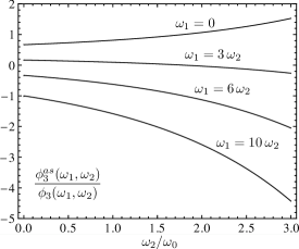
Figure 1: The ratio $\phi^{\rm as}_{3}/\phi_{3}$ as a function of $\omega_{2}/\omega_{0}$ for several values of $\omega_{1}/\omega_{0}$ for the model in Eq. (63).

The quark-gluon DA at higher scales is given by

$$\phi_{3}(\omega_{1},\omega_{2},\mu) =\frac{1}{2i}\int\limits_{0}^{\infty}ds\,R(s;\mu,\mu_{0})\int_{C}dx\,x\,\tan\pi x\,\left(x^{2}-\frac{9}{4}\right)\mathbb{Y}_{s,x}(\omega_{1},\omega_{2})L^{\gamma_{-ix}/\beta_{0}}\langle{\mathbb{Y}_{s,x}|\Phi_{3}}\rangle\,,$$ (69)

where the $x-$integration goes along the imaginary axis with $\text{Re}(x)=-1$. For numerical evaluation it is convenient to consider first the corresponding function in the $(s,u)$-representation (LABEL:tildePsi),

$$\bar{u}\,\widetilde{\phi}_{3}(s,u,\mu)=-\frac{1}{2is^{2}}R(s;\mu,\mu_{0})\int_{C}dx\,x\,\tan\pi x\,\left(x^{2}-\frac{9}{4}\right)\,{}_{2}F_{1}\left(\genfrac{}{}{0.0pt}{}{-\frac{1}{2}-x,-\frac{1}{2}+x}{2}\Big{|}-\frac{u}{\bar{u}}\right)L^{\gamma_{-ix}/\beta_{0}}\langle{\mathbb{Y}_{s,x}|\Phi_{3}}\rangle\,,$$ (70)

and calculate the DA in momentum space as

$$\phi(\omega_{1},\omega_{2})=\int_{0}^{\infty}ds\,s\int_{0}^{1}du\,(\omega_{1}su)^{1/2}\,(\omega_{2}s\bar{u})\,J_{1}\left(2\sqrt{us\omega_{1}}\right)J_{2}\left(2\sqrt{\bar{u}s\omega_{2}}\right)\,\widetilde{\phi}_{3}(s,u,\mu)\,.$$ (71)

For our model (63)

$$\langle{\mathbb{Y}_{s,x}|\Phi_{3}}\rangle =\frac{1}{3}\varphi_{3}s^{2}e^{-\omega_{0}s}\frac{\pi}{\cos\pi x}\left(x^{2}-\frac{1}{4}\right)\,$$ (72)

and the function $\widetilde{\phi}_{3}(s,u,\mu)$ has a factorized form

$$\bar{u}\,\widetilde{\phi}_{3}(s,u,\mu)=\varphi_{3}R(s;\mu,\mu_{0})e^{-\omega_{0}s}W(u,\mu)\,,$$ (73)

where

$$W(u,\mu) =\frac{i}{6}\int_{C}dx\,\frac{\pi x\sin\pi x}{\cos^{2}\pi x}\,\,\left(x^{2}-\frac{9}{4}\right)\left(x^{2}-\frac{1}{4}\right)$$

$$\times{}_{2}F_{1}\left(\genfrac{}{}{0.0pt}{}{-\frac{1}{2}-x,-\frac{1}{2}+x}{2}\Big{|}-\frac{u}{\bar{u}}\right)L^{\gamma_{-ix}/\beta_{0}}.$$ (74)

The function $W(u,\mu)\propto\bar{u}\,\widetilde{\phi}_{3}(s,u,\mu)$ at three different scales $\mu=\mu_{0}=1\,\text{GeV}$, $\mu=2.5\,\text{GeV}$ and $\mu=10\,\text{GeV}$ is shown in Fig. 2.

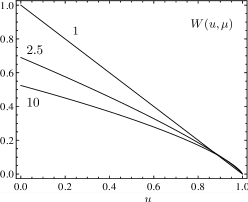
Figure 2: The function $W(u,\mu)$, Eq. (IV), on three different scales $\mu=\mu_{0}=1\,\text{GeV}$, $\mu=2.5\,\text{GeV}$ and $\mu=10\,\text{GeV}$.

Note that $u$ and $\bar{u}=1-u$ have the meaning of the momentum fractions carried by the quark and the gluon, respectively:

$$\omega_{1}=u\omega\,, \omega_{2}=\bar{u}\omega\,, \omega=\omega_{1}+\omega_{2}\,,$$ (75)

so that the scale dependence visualized in Fig. 2 corresponds to a redistribution of the total momentum of the light degrees of freedom such that at large scales the gluon carries a larger fraction. Note also that $W(u,\mu)$ becomes slightly curved at $u\to 1$ but still vanishes, or, equivalently, the DA $\widetilde{\phi}_{3}(s,u,\mu)$ diverges in the same limit, but the divergence is softer than a power $1/\bar{u}$.

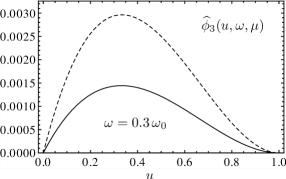
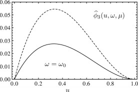
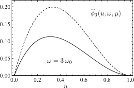
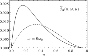
Figure 3: The three-particle B-meson DA (76) as a function of the quark momentum fraction $u$ after the evolution to $\mu=2.5$ GeV (solid curves) and at the initial scale $\mu=\mu_{0}=1$ GeV (dashed curves) for the model in Eq. (63) for several values of the total momentum $\omega=\omega_{1}+\omega_{2}$.

Finally, we show in Fig. 3 the (normalized) DA in momentum space

$$\widehat{\phi}_{3}(u,\omega,\mu)=\frac{\omega_{0}^{2}}{\varphi_{3}}\phi_{3}(u\omega,\bar{u}\omega,\mu)$$ (76)

as a function of the quark momentum fraction after the evolution to $\mu=2.5$ GeV (solid curves) and at the initial scale $\mu=\mu_{0}=1$ GeV (dashed curves) for four different values of the total momentum $\omega/\omega_{0}=\{0.3,1,3,9\}$.

One sees that for small total momentum the DA is rather strongly suppressed by the evolution whereas the shape is only weakly affected. On the contrary, for large momentum there is no suppression and the DA is strongly tilted towards small values of $u$, corresponding to small quark and large gluon momenta. It would be interesting to analyze the large-momentum behavior using the expansion of the type suggested in Lee:2005gza (see also Feldmann:2014ika ). Such a study goes, however, beyond the tasks of this paper.

V Conclusions

To summarize, we have shown that the evolution equation for the three-particle quark-gluon B-meson light-cone DA of subleading twist is completely integrable in the large $N_{c}$ limit and can be solved exactly in analytic form. The most important result for phenomenology is that “genuine” three-particle contributions of quark-gluon states essentially decouple from the subleading-twist two-particle DA $\phi_{-}(\omega)$ Beneke:2000wa so that its properties are similar to the leading-twist DA. A similar simplification has been found before for the structure function $g_{2}(x,Q^{2})$ in polarized deep-inelastic lepton-hadron scattering Ali:1991em ; Balitsky:1996uh ; Braun:2000av ; Braun:2001qx . Based on this experience, we expect that “genuine” three-particle contributions do not contribute directly to many physical observables in B-decays at tree level because three-particle and two-particle twist-three contributions to the products of currents are typically related by Ward identities; hence they cannot have a different scale dependence. We also expect that a similar simplification of the renormalization-group dependence holds for twist-four distributions as well. This study is in progress BM . In this way we hope to be able to identify important degrees of freedom in multiparticle quark-gluon distributions in heavy mesons that can be parametrized by a minimum number of nonperturbative parameters. This would present a step forward towards understanding of subleading corrections in powers of the heavy quark mass and ultimately allow one to increase significantly the accuracy of QCD predictions for heavy meson (and baryon) decays based on the heavy-quark expansion and/or light-cone sum rules.

References

(1)
M. Beneke, G. Buchalla, M. Neubert and C. T. Sachrajda,
Phys. Rev. Lett. 83 (1999) 1914;
Nucl. Phys. B 591 (2000) 313.
(2)
M. Beneke and T. Feldmann,
Nucl. Phys. B 592 (2001) 3.
(3)
A. G. Grozin and M. Neubert,
Phys. Rev. D 55 (1997) 272.
(4)
B. O. Lange and M. Neubert,
Phys. Rev. Lett. 91 (2003) 102001.
(5)
V. M. Braun, D. Yu. Ivanov and G. P. Korchemsky,
Phys. Rev. D 69 (2004) 034014.
(6)
S. J. Lee and M. Neubert,
Phys. Rev. D 72 (2005) 094028.
(7)
G. Bell, T. Feldmann, Y.-M. Wang and M. W. Y. Yip,
JHEP 1311 (2013) 191.
(8)
V. M. Braun and A. N. Manashov,
Phys. Lett. B 731, 316 (2014).
(9)
T. Feldmann, B. O. Lange and Y. M. Wang,
Phys. Rev. D 89 (2014) 11, 114001.
(10)
A. Khodjamirian, T. Mannel and N. Offen,
Phys. Rev. D 75 (2007) 054013.
(11)
F. De Fazio, T. Feldmann and T. Hurth,
JHEP 0802 (2008) 031.
(12)
V. M. Braun and A. Khodjamirian,
Phys. Lett. B 718, 1014 (2013).
(13)
Y. M. Wang and Y. L. Shen,
arXiv:1506.00667 [hep-ph].
(14)
H. Kawamura, J. Kodaira, C. F. Qiao and K. Tanaka,
Phys. Lett. B 523 (2001) 111
[Erratum-ibid. B 536 (2002) 344].
(15)
T. Nishikawa and K. Tanaka,
Nucl. Phys. B 879 (2014) 110.
(16)
A. Ali, V. M. Braun and G. Hiller,
Phys. Lett. B 266 (1991) 117.
(17)
I. I. Balitsky, V. M. Braun, Y. Koike and K. Tanaka,
Phys. Rev. Lett. 77 (1996) 3078.
(18)
V. M. Braun, G. P. Korchemsky and A. N. Manashov,
Phys. Lett. B 476 (2000) 455.
(19)
V. M. Braun, G. P. Korchemsky and A. N. Manashov,
Nucl. Phys. B 603 (2001) 69.
(20)
M. Knödlseder and N. Offen,
JHEP 1110 (2011) 069.
(21) I.M. Gelfand, M.I. Graev, N.Ya. Vilenkin, “Generalized functions. Vol. 5: Integral geometry and
representation theory,” Academic Press (New York, 1966).
(22)
A. P. Bukhvostov, G. V. Frolov, L. N. Lipatov and E. A. Kuraev,
Nucl. Phys. B 258 (1985) 601.
(23)
V. M. Braun, A. N. Manashov and B. Pirnay,
Phys. Rev. D 80, 114002 (2009)
[Erratum-ibid. D 86, 119902 (2012)].
(24)
L. D. Faddeev, E. K. Sklyanin and L. A. Takhtajan,
Theor. Math. Phys. 40, 688 (1980).
(25)
V. M. Braun and A. N. Manashov, work in progress.
(26)
E. K. Sklyanin, “Quantum inverse scattering method. Selected
topics”, “Quantum Group and Quantum Integrable Systems” (Nankai Lectures in Mathematical Physics), ed. Mo-Lin Ge,
Singapore: World Scientific, 1992, pp. 63–97,
hep-th/9211111.
(27)
S. E. Derkachov, G. P. Korchemsky and A. N. Manashov,
JHEP 0310 (2003) 053.
(28)
S. E. Derkachov, G. P. Korchemsky and A. N. Manashov,
Nucl. Phys. B 566 (2000) 203.
(29)
A. M. Polyakov,
Nucl. Phys. B 164 (1980) 171.
(30)
G. P. Korchemsky and A. V. Radyushkin,
Nucl. Phys. B 283 (1987) 342.