Abstract

In this Chapter we provide an overview of the current first-principles perspective on flexoelectric effects in crystalline solids. We base our theoretical formalism on the long-wave expansion of the electrical response of a crystal to an acoustic phonon perturbation. In particular, we recover the known expression for the piezoelectric tensor from the response at first order in wavevector ${\bf q}$, and then obtain the flexoelectric tensor by extending the formalism to second order in $\bf q$. We put special emphasis on the issue of surface effects, which we first analyze heuristically, and then treat more carefully by presenting a general theory of the microscopic response to an arbitrary inhomogeneous strain. We demonstrate our approach by presenting a full calculation of the flexoelectric response of a SrTiO₃ film, where we point out an unusually strong dependence of the bending-induced open-circuit voltage on the choice of surface termination. Finally, we briefly discuss some remaining open issues concerning the methodology and some promising areas for future research.

Chapter 0 First-principles theory of flexoelectricity

1 Introduction

First-principles electronic structure calculations have played an increasingly important role in our understanding of the properties of materials and nanostructures in recent decades. The phrase “first principles” is generally used in the condensed-matter community to convey the notion that the calculations are free of adjustable parameters, taking as input only some list of atoms, their atomic numbers, and some initial guesses at their coordinates in the unit cell. One then solves the Schrödinger equation for the electrons in some approximation, computes the relaxed atomic coordinates, and calculates the desired properties of the crystal. In the condensed-matter community this is typically done in the framework of density-functional theory (DFT),[1] as shall be assumed below, but Hartree-Fock or other quantum-chemical methods can also be used.

While the accuracy and efficiency of DFT methods have improved over the years, of equal importance has been the increasing range of quantities that can be computed. In the context of dielectric properties, the implementation of linear-response theory for phonon and electric-field perturbations in the 1980s and 1990s opened up the calculation of phonon frequencies, dynamical charges, and both electronic and lattice contributions to the dielectric constant.[2] While there was initially some doubt about whether the piezoelectric response was a bulk property at all, a seminal paper of Martin laid this question to rest,[3] and the computation of the piezoelectric tensor is now a standard feature of most DFT codes as well. Strangely, although many of the above properties can be computed as derivatives of the electric polarization $\bf P$, a proper definition of the polarization $\bf P$ itself proved more difficult; the physics was clarified, and practical methods for computing it, were developed only in the mid-1990s with the appearance of the “modern theory of polarization.”[4, 5, 6] Related methods for computing the orbital magnetization of ferromagnets and the properties of crystals in finite electric fields have been developed since the 2000’s.[7]

The flexoelectric tensor has been among the few physical properties to have resisted a proper first-principles formulation even until today. The theory of flexoelectricity was pioneered in the 1980s by Tagantsev.[8, 9] However, because it encodes a response to a strain gradient, rather than just a strain, and because a strain gradient is inconsistent with ordinary cell-periodic boundary conditions, methods based on Bloch’s theorem cannot be straightforwardly applied in the first-principles context. A serious attack on this problem did not begin until 2010, when Hong and collaborators presented the results of calculations on supercell configurations containing strain gradients.[10] Subsequent papers of Resta[11] and Hong and Vanderbilt[12] clarified aspects of the electronic contribution to the flexoelectric response.

More recently, Stengel[13] and Hong and Vanderbilt[14] tackled the problem in a systematic way, and working from slightly different perspectives, arrived consistently at a nearly complete framework for defining, and eventually computing, the flexoelectric tensors fully from first-principles. Some components of the flexoelectric tensor that can be expressed only in terms of bulk current responses, as opposed to charge responses, still require care in their interpretation and await the development of efficient methods for calculating them. However, we can expect these difficulties to be cleared up soon, so we can look forward to a new era in which first-principles calculations of flexoelectric responses can flourish and contribute to a fast-evolving experimental field. The purpose of this chapter is to outline the physical principles underlying these advances in the understanding and computation of flexoelectric responses, and to summarize a few of the preliminary results that have been presented in the literature to date.

2 Theory and methods

1 Strain, strain gradients, and responses

We begin by establishing our notation. In continuum mechanics, a deformation can be expressed as a three-dimensional (3D) vector field, $u_{\alpha}({\bf r})$, describing the displacement of a material point from its reference position at ${\bf r}$ to its current location ${\bf r}^{\prime}$, 

$$r_{\alpha}^{\prime}({\bf r})=r_{\alpha}+u_{\alpha}({\bf r}),$$

The deformation gradient is defined as the gradient of $u_{\alpha}$ taken in the reference configuration,

$$\tilde{\varepsilon}_{\alpha\beta}({\bf r})=u_{\alpha,\beta}({\bf r})=\frac{\partial u_{\alpha}({\bf r})}{\partial r_{\beta}}.$$ (1)

$\tilde{\varepsilon}_{\alpha\beta}({\bf r})$ is often indicated in the literature as “unsymmetrized strain tensor”, as it generally contains a proper strain plus a rotation. By symmetrizing its indices one can remove the rotational component, thus obtaining the symmetrized strain tensor

$$\varepsilon_{\alpha\beta}=\frac{1}{2}\left(u_{\alpha,\beta}+u_{\beta,\alpha}\right).$$

This $\varepsilon_{\alpha\beta}$ is a convenient measure of local strain, as it only depends on relative displacements of two adjacent material points, and not on their absolute translation or rotation with respect to some reference configuration.

In this work we shall be primarily concerned with the effects of a spatially inhomogeneous strain. The third-rank strain gradient tensor can be defined in two different ways, both important for the derivations that follow. The first (type-I) form consists in the gradient of the unsymmetrized strain,

$$\eta_{\alpha,\beta\gamma}({\bf r})=\frac{\partial\tilde{\varepsilon}_{\alpha\beta}({\bf r})}{\partial r_{\gamma}}=\frac{\partial^{2}u_{\alpha}({\bf r})}{\partial r_{\beta}\partial r_{\gamma}}.$$ (2)

Note that $\eta_{\alpha,\beta\gamma}$, manifestly invariant upon $\beta\leftrightarrow\gamma$ exchange, corresponds to the $\nu_{\alpha\beta\gamma}$ tensor of Ref. 12, and to the symbol $\partial\epsilon_{\alpha\beta}/\partial r_{\gamma}$ of Ref. 8. Alternatively, the strain gradient tensor can be defined (type-II) as the gradient of the symmetric strain, $\varepsilon_{\alpha\beta}$,

$$\varepsilon_{\alpha\beta,\gamma}({\bf r})=\frac{\partial\varepsilon_{\alpha\beta}({\bf r})}{\partial r_{\gamma}},$$

invariant upon $\alpha\leftrightarrow\beta$ exchange. It is straightforward to verify that the two tensors contain exactly the same number of independent entries, and that a one-to-one relationship can be established to express the former as a function of the latter and vice versa,

$$\eta_{\alpha,\beta\gamma}=\varepsilon_{\alpha\beta,\gamma}+\varepsilon_{\gamma\alpha,\beta}-\varepsilon_{\beta\gamma,\alpha}.$$ (3)

The piezoelectric and flexoelectric tensors describe, respectively, the macroscopic polarization response to a uniform strain and to a strain gradient. In type-I form, these are

$$e_{\alpha\beta\gamma} = \frac{dP_{\alpha}}{d\varepsilon_{\beta\gamma}},$$ (4)

$$\mu^{\rm I}_{\alpha\beta,\gamma\lambda} = \frac{dP_{\alpha}}{d\eta_{\beta,\gamma\lambda}}.$$ (5)

While the type-I form is more convenient to derive and calculate, the type-II representation is often preferred in applications. The type-II flexoelectric tensor is defined as

$$\mu^{\rm II}_{\alpha\lambda,\beta\gamma}=\frac{\partial P_{\alpha}}{\partial\varepsilon_{\beta\gamma,\lambda}}.$$ (6)

Note that $\mu^{\rm I}$ and $\mu^{\rm II}$ are both symmetric under the last two indices, and are related to each other via Eq. (3) according to

$$\mu^{\rm II}_{\alpha\lambda,\beta\gamma} = \mu^{\rm I}_{\alpha\beta,\gamma\lambda}+\mu^{\rm I}_{\alpha\gamma,\lambda\beta}-\mu^{\rm I}_{\alpha\lambda,\beta\gamma},$$ (7)

$$\mu^{\rm I}_{\alpha\beta,\gamma\lambda} = \frac{1}{2}\,\left(\mu^{\rm II}_{\alpha\lambda,\beta\gamma}+\mu^{\rm II}_{\alpha\gamma,\beta\lambda}\right).$$ (8)

2 Long-wave approach

A macroscopic strain gradient breaks the translational symmetry of the crystal lattice. For this reason, the response to such a perturbation cannot be straightforwardly represented in periodic boundary conditions. This makes the theoretical study of flexoelectricity more challenging than other forms of electromechanical couplings such as piezoelectricity. To circumvent this difficulty, we shall base our analysis on the study of long-wavelength acoustic phonons. These perturbations, while generally incommensurate with the crystal lattice, can be conveniently described in terms of functions that are lattice-periodic, and therefore are formally and computationally very advantageous.[2]

Consider a crystal lattice spanned by the real-space translation vectors ${\bf R}_{l}$ and by the basis vectors ${\bm{\tau}}_{\kappa}$, in such a way that ${\bf R}_{l\kappa}={\bf R}_{l}+{\bm{\tau}}_{\kappa}$ indicates the location of the atom of sublattice $\kappa$ and cell $l$. In full generality, the atomic displacements along the Cartesian direction $\alpha$ associated with a phonon eigenmode of wavevector ${\bf q}$ can be written as

$$u_{\kappa\alpha}(l,t)=u^{\bf q}_{\kappa\alpha}\,e^{i{\bf q}\cdot{\bf R}_{l\kappa}-i\omega t},$$ (9)

where $u^{\bf q}_{\kappa\alpha}$ (independent of either $l$ or $t$) is an eigenvector of the dynamical matrix at ${\bf q}$, and $\omega$ is the frequency.

A convenient description of arbitrary mechanical deformations can be established by choosing an acoustic phonon branch, and by performing a long-wave (small ${\bf q}$) expansion of its eigenvector in the vicinity of the $\Gamma$ point. Provided that the long-range electrostatic fields are adequately screened (see Sec. 3 for a discussion), the aforementioned expansion can be written as

$$u^{\bf q}_{\kappa\alpha}=U_{\alpha}\left(\delta_{\alpha\beta}+iq_{\gamma}\Gamma^{\kappa}_{\alpha\beta\gamma}-q_{\gamma}q_{\lambda}N^{\kappa}_{\alpha\beta\gamma\lambda}+\ldots\right),$$ (10)

where ${\bf U}$ is a Cartesian vector, $\delta_{\alpha\beta}$ is the Kronecker delta, and $\Gamma^{\kappa}_{\alpha\beta\gamma}$ and $N^{\kappa}_{\alpha\beta\gamma\lambda}$ are third- and fourth-order tensors, respectively. (The dots stand for higher-order terms, which are irrelevant in the context of the phenomena described here.) At order zero in ${\bf q}$ the phonon eigenmode is a rigid translation of the whole lattice along ${\bf U}$ (note the absence of a sublattice index), while the first- and second-order terms describe the internal-strain response of the lattice to a uniform strain or to a macroscopic strain gradient, respectively.

Of course, to obtain the relevant electromechanical coupling coefficients, the sole knowledge of the lattice distortions is not sufficient – one needs to establish a link between atomic displacements and macroscopic polarization. While in a simplified point-charge model such a link is straightforward, in the case of a more realistic quantum-mechanical description of a solid things are significantly more involved, as one needs to understand how the electronic wavefunctions, and not only the nuclei, respond to a macroscopic deformation. If the deformation is sufficiently slow, which is the case of the phenomena described in this chapter, the electronic cloud responds adiabatically to atomic motion by generating a microscopic current density (i.e., the quantum-mechanical probability current). For example, if we displace by hand one atomic sublattice as

$$u_{\kappa\beta}(l,t)=\lambda(t)e^{i{\bf q}\cdot{\bf R}_{l\kappa}}$$ (11)

the microscopic current density that is linearly induced by such a perturbation can be written as 

$${\bf J}({\bf r},t)=\dot{\lambda}(t)\,{\bf P}_{\kappa\beta}^{\bf q}({\bf r})\,e^{i{\bf q}\cdot{\bf r}}.$$ (12)

The function ${\bf P}_{\kappa\beta}^{\bf q}({\bf r})$ is the microscopic polarization response; its cell average,

$$\overline{\bf P}_{\kappa\beta}^{\bf q}=\frac{1}{\Omega}\int_{\rm cell}d^{3}r{\bf P}_{\kappa\beta}^{\bf q}({\bf r}),$$ (13)

where $\Omega$ is the cell volume, describes the contribution of atomic motion to the macroscopic polarization, which is the quantity we are ultimately interested in.

To go from here to the electromechanical tensors we need one more step, i.e., the small-${\bf q}$ expansion of $\overline{\bf P}_{\kappa\beta}^{\bf q}$. Again expanding in powers of $\bf q$ and keeping terms up to second order, 

$$\overline{\bf P}_{\kappa\beta}^{\bf q}=\overline{\bf P}^{(0)}_{\kappa\beta}-iq_{\gamma}\overline{\bf P}^{(1,\gamma)}_{\kappa\beta}-\frac{q_{\gamma}q_{\lambda}}{2}\overline{\bf P}^{(2,\gamma\lambda)}_{\kappa\beta}+\ldots.$$ (14)

The zero-th order term is the macroscopic polarization response to a macroscopic translation of the sublattice $\kappa$ along the direction $\beta$. This corresponds precisely to the definition of the Born dynamical charge tensor $Z^{*}$,

$$\overline{P}^{(0)}_{\alpha\,\kappa\beta}=\frac{Z^{*}_{\kappa,\alpha\beta}}{\Omega}.$$ (15)

The remaining ${\bf P}$-tensors can be regarded as higher-order counterparts of the Born charges. (Physically they are directly related to the moments of the current density induced by the displacement of an isolated atom. [13, 14])

Multiplying the lattice-polarization coupling tensors with the phonon eigendisplacements, we can collect terms order-by-order in $\bf q$. The zero-order term (rigid translation) vanishes due to the acoustic sum rule. At first order in ${\bf q}$, we obtain the explicit expression for the piezoelectric tensor[15]

$$e_{\alpha\beta\gamma} = -\sum_{\kappa}\overline{P}_{\alpha,\kappa\beta}^{(1,\gamma)}+\frac{Z^{*}_{\kappa,\alpha\rho}}{\Omega}\Gamma^{\kappa}_{\rho\beta\lambda},$$ (16)

where the first and second terms are the electronic (frozen-ion) and lattice-mediated terms respectively.  Collecting the terms at second order in $\bf q$ gives the flexoelectric response, which is again a sum

$$\mu^{\rm I}_{\alpha\beta,\gamma\lambda}=\bar{\mu}^{\rm I}_{\alpha\beta,\gamma\lambda}+\mu^{\rm I,mix}_{\alpha\beta,\gamma\lambda}+\mu^{\rm I,latt}_{\alpha\beta,\gamma\lambda},$$ (17)

of electronic and lattice terms

$$\bar{\mu}^{\rm I}_{\alpha\beta,\gamma\lambda} = \frac{1}{2}\sum_{\kappa}\overline{P}_{\alpha,\kappa\beta}^{(2,\gamma\lambda)},$$ (18)

$$\mu^{\rm I,mix}_{\alpha\beta,\gamma\lambda} = -\frac{1}{2}\left(\Gamma^{\kappa}_{\rho\beta\gamma}\overline{P}_{\alpha,\kappa\rho}^{(1,\lambda)}+\Gamma^{\kappa}_{\rho\beta\lambda}\overline{P}_{\alpha,\kappa\rho}^{(1,\gamma)}\right),$$ (19)

$$\mu^{\rm I,latt}_{\alpha\beta,\gamma\lambda} = \frac{Z^{*}_{\kappa,\alpha\rho}}{\Omega}N^{\kappa}_{\rho\beta\gamma\lambda},$$ (20)

where the bar symbol on the first term indicates a purely electronic response and ‘mix’ and ‘latt’ refer to “mixed” and “lattice-mediated” contributions, respectively. While the piezoelectric and flexoelectric responses have been developed in parallel until now, we will henceforth concentrate on the latter, referring the reader to Refs. [13, 14] for the detailed treatment of the piezoelectric response. The corresponding type-II flexoelectric responses are

$$\mu^{\rm II}_{\alpha\lambda,\beta\gamma}=\bar{\mu}^{\rm II}_{\alpha\lambda,\beta\gamma}+\mu^{\rm II,mix}_{\alpha\lambda,\beta\gamma}+\mu^{\rm II,latt}_{\alpha\lambda,\beta\gamma},$$ (21)

where

$$\bar{\mu}^{\rm II}_{\alpha\lambda,\beta\gamma} = \frac{1}{2}\sum_{\kappa}\left(\overline{P}_{\alpha,\kappa\beta}^{(2,\gamma\lambda)}+\overline{P}_{\alpha,\kappa\gamma}^{(2,\lambda\beta)}-\overline{P}_{\alpha,\kappa\lambda}^{(2,\beta\gamma)}\right),$$ (22)

$$\mu^{\rm II,mix}_{\alpha\lambda,\beta\gamma} = -\Gamma^{\kappa}_{\rho\beta\gamma}\overline{P}_{\alpha,\kappa\rho}^{(1,\lambda)},$$ (23)

$$\mu^{\rm II,latt}_{\alpha\lambda,\beta\gamma} = \frac{Z^{*}_{\kappa,\alpha\rho}}{\Omega}\left(N^{\kappa}_{\rho\beta,\lambda\gamma}+N^{\kappa}_{\rho\gamma,\lambda\beta}-N^{\kappa}_{\rho\lambda,\beta\gamma}\right).$$ (24)

For later convenience we rewrite Eq. (24) as

$$\mu^{\rm II,latt}_{\alpha\lambda,\beta\gamma}=\frac{Z^{*}_{\kappa,\alpha\rho}}{\Omega}L^{\kappa}_{\rho\lambda,\beta\gamma}$$ (25)

where $L^{\kappa}_{\rho\lambda,\beta\gamma}$ (the type-II counterpart of the type-I internal-strain tensor ${\bf N}$) is the quantity in parentheses on the right-hand side of Eq. (24).

To summarize, according to Eq. (9) a long-wavelength sound wave is comprised of a lattice-periodic distortion pattern $u_{\kappa\alpha}^{\bf q}$ modulated by a time- and space-dependent complex phase factor. At zero order in $\bf q$ the deformation can be described as purely “elastic,” but at higher orders (i.e., when moving away from the zone center), internal relaxations of the basis atoms in the primitive cell occur, as described by the tensors $\bm{\Gamma}$ and ${\bf N}$ (or $\bf L$) at first and second orders in $\bf q$, respectively. These are related to how the crystal locally responds to a macroscopic strain (first order, “piezo”) or strain gradient (second order, “flexo”). The reader is referred to Refs. [13, 14] for the derivation of explicit expressions for these tensors, but we shall highlight the main conceptual issues associated with them in Sec. 4. Each consecutive order in Eq. (10) gives rise to a corresponding term in the expressions for the flexoelectric tensor in Eqs. (17) and (21).

Regarding the purely electronic term, $\bar{\bm{\mu}}$, which is associated with the purely elastic part (order-zero in $\bf q$, also referred to as “frozen ion deformation”), we defer its detailed discussion to Section 5. It can be shown that the “mixed” $\mu^{\rm II,mix}_{\alpha\lambda,\beta\gamma}$ term involving $\Gamma^{\kappa}_{\rho\beta\gamma}$ is active only in crystals that are characterized by Raman-active phonons,[14] which is not the case for simple systems such as cubic rocksalt or perovskite crystals. (Again, we refer the reader to Refs. [13, 14] for the explicit discussion of this term.) By contrast, the $\mu^{\rm II,latt}_{\alpha\lambda,\beta\gamma}$ term is present in any insulator with IR-active phonons; as this term is very important in practical applications of the flexoelectric effect, we shall discuss it shortly in Sec. 4. First, however, we shall briefly comment on an important issue that is relevant to the above discussion, concerning the treatment of the macroscopic electric fields in the long-wave phonon analysis.

3 Macroscopic electric fields

Depending on their polarity, long-wave phonons in a crystalline insulator generally produce macroscopic electric fields. These are due to the charge perturbation that is generated by the lattice distortion, and have a nonanalytic behavior in the vicinity of the $\Gamma$ point. For example, for a monochromatic perturbation such as that of Eq. (11), at the lowest order in ${\bf q}$ the macroscopic electric field tends to a direction-dependent constant,

$$\overline{\bf E}^{{\bf q}\rightarrow 0}_{\kappa\beta}\sim-\frac{{\bf q}}{\epsilon_{0}\Omega}\frac{({\bf q}\cdot{\bf Z}^{*})_{\kappa\beta}}{{\bf q}\cdot\bar{\bm{\epsilon}}_{\rm r}\cdot{\bf q}},$$ (26)

where $\overline{\bf E}^{\bf q}_{\kappa\beta}$ is defined in analogy with Eq. (13) and $\bar{\bm{\epsilon}}_{\rm r}$ is the purely electronic relative permittivity tensor. The main physical consequence of this is the well-known frequency splitting between longitudinal optical (LO) and transverse optical (TO) phonons in polar crystals. In particular, due to the contribution of Eq. (26) to the dynamical matrix, the LO dispersion curves behave nonanalytically already at zero order in ${\bf q}$; that is, the eigenvalue and eigenvector associated with an LO branch generally depends on the direction along which one approaches $\Gamma$. Such a nonanaliticity propagates directly to the electronic and lattice response functions described in the previous Section, and needs to be adequately treated in order to be able to apply the Taylor expansions described in Eq. (10) and (14). 

There are several ways to approach this problem. For example, the theory of Ref. 14 was developed for purely transverse and longitudinal phonons separately, leading to flexoelectric coefficients defined at fixed $\bf E$ and $\bf D$ (electric displacement field) respectively. Here, we take the approach of removing the macroscopic ${\bf E}$-fields  in a physically meaningful way by assuming, following Martin, [3] that a very low density of free carriers is present in the insulating crystal, and that these are allowed to redistribute adiabatically in response to a phonon perturbation. In particular, within the Thomas-Fermi approximation, we write the free-carrier density as

$$\rho^{\rm free}({\bf r})=-\epsilon_{0}k_{\rm TF}^{2}V({\bf r}),$$ (27)

where $V({\bf r})$ is as usual the electrostatic potential, and we suppose that the Fermi wavevector $k_{\rm TF}$ is much smaller than any reciprocal lattice vector of the crystal. In such a regime, the ground-state charge density and wavefunctions are essentially unaffected by the additional screening provided by the free-electron gas. Conversely, in the long-wave limit, the presence of the free carriers drastically alters the electrostatics; for example, the field of Eq. (26) becomes [13]

$$\overline{\bf E}^{{\bf q}\rightarrow 0}_{\kappa\beta}\sim-\frac{{\bf q}}{\epsilon_{0}\Omega}\frac{({\bf q}\cdot{\bf Z}^{*})_{\kappa\beta}}{k_{\rm TF}^{2}+{\bf q}\cdot\bar{\bm{\epsilon}}_{\rm r}\cdot{\bf q}}.$$ (28)

Such a modification has the following effects:

• The macroscopic electric fields, and hence all the response properties of the crystal, become analytic functions of ${\bf q}$.

• The macroscopic electric fields vanish at zero and first order in ${\bf q}$, and also at second order in $\bf q$ provided that we are considering an acoustic phonon branch.

• Both the piezoelectric and flexoelectric tensors calculated in the presence of the free carrier gas are independent of $k_{\rm TF}$, and therefore can be unambiguously interpreted as the short-circuit versions of the corresponding electromechanical response functions.

In the first-principles calculations, this is done in practice by simply suppressing the ${\bf G}=0$ contribution to the electrostatic energy when computing the self-consistent linear response; this has the same effect as introducing a low-density electron gas as described above.

Based on the above discussion, it would be tempting to conclude that the flexoelectric tensor, like the piezoelectric tensor, is well defined under short-circuit electrical boundary conditions. In writing down Eq. (27), however, we assumed a particular type of carriers, namely electrons (not holes), and moreover that the band edge for those carriers, the conduction-band minimum (CBM), tracks with the macroscopic electrostatic potential of the crystal. In general, however, the CBM energy may shift relative to the local macroscopic potential as a result of a strain gradient, via the so-called deformation-potential effect. Thus, we can obtain a different flexoelectric tensor depending on what band feature (CBM or other) we choose as the energy reference. We shall come back to this point in Sec. 5.

For a given energy reference, the bulk flexoelectric tensor $\bm{\mu}$ is well defined in short-circuit (fixed ${\bf E}$) boundary conditions. If fixed ${\bf D}$ boundary conditions are imposed along a specific direction $\hat{\bf q}$, the induced electric field (defined as the tilt of the corresponding reference potential) can be then easily calculated as 

$${\bf\Delta E}^{\rm bulk}=-\frac{{\bf q}}{\epsilon_{0}}\frac{q_{\alpha}\,\mu^{\rm II}_{\alpha\lambda,\beta\gamma}\,\varepsilon_{\beta\gamma,\lambda}}{{\bf q}\cdot\bm{\epsilon}_{\rm r}\cdot{\bf q}}.$$ (29)

Note that Eq. (29) cannot be written in tensorial form, except for the simplest case of crystals with cubic symmetry, where the denominator reduces to a direction-independent constant.

4 Lattice response

To gain some insight into the nature of the lattice-mediated flexoelectric effect it is necessary to understand, in broad terms, the physics behind the internal-strain response (as described by the tensors ${\bf N}$ or ${\bf L}$) to a strain gradient deformation. To that end, suppose that we perform a computational experiment where we statically freeze in a lattice distortion that corresponds to an acoustic  phonon truncated to first order in ${\bf q}$, i.e., to the uniform-strain level,

$$u^{l}_{\kappa\alpha}=\left(\delta_{\alpha\beta}+iq_{\gamma}\Gamma^{\kappa}_{\alpha\beta\gamma}\right)U_{\beta}e^{i{\bf q\cdot R}_{l\kappa}}.$$ (30)

(In the simplest crystal structures, where the $\bm{\Gamma}$ tensor identically vanishes, this corresponds to a purely elastic wave.) As we have perturbed the crystal from its equilibrium configuration, each atom in the lattice (identified, as usual, by a cell index $l$ and a basis index $\kappa$) will experience a restoring force $f^{l}_{\kappa\alpha}$. If the amplitude of the deformation is small (linear-response regime), such forces can be described, as usual, by a lattice-periodic (i.e., $l$-independent) function that is modulated by a complex phase with the same wavevector ${\bf q}$ as the perturbation. For small ${\bf q}$, it can be shown that the magnitude of the induced forces scales as $\mathcal{O}(q^{2})$ (first-order terms cannot be present, as we have assumed that uniform-strain effects are already included), and can be written as

$$f^{l}_{\kappa\alpha}\sim-q_{\gamma}q_{\lambda}U_{\beta}T^{\kappa}_{\alpha\beta,\gamma\lambda}e^{i{\bf q\cdot R_{l\kappa}}}.$$ (31)

Here $T^{\kappa}_{\alpha\beta,\gamma\lambda}$ is, by construction, the type-I flexoelectric force-response tensor. (The detailed derivation can be found in Ref. [13, 14].)

Now one would be tempted, in close analogy to the piezoelectric case, to define the internal-strain response tensor ${\bf N}$ by means of the following linear system of equations,

$$\Phi^{(0)}_{\kappa\alpha\kappa^{\prime}\rho}N^{\kappa^{\prime}}_{\rho\beta,\gamma\lambda}\stackrel{{\scriptstyle?}}{{=}}T^{\kappa}_{\alpha\beta,\gamma\lambda},$$ (32)

where $\Phi^{(0)}_{\kappa\alpha\kappa^{\prime}\rho}$ is the zone-center force-constant matrix.  Unfortunately, the above system is generally not solvable: the sublattice- ($\kappa$-) sum of the ${\bf T}$-tensor does not vanish, and the $\Phi^{(0)}$ matrix is singular. (It is always characterized by three null eigenvalues, corresponding to rigid translations of the crystal as a whole.) As negative as it sounds, this is nonetheless an important result: it tells us that the internal-strain response to a static strain-gradient deformation is generally ill-defined. (We shall see later on that there are notable exceptions to this statement, though.)

To understand what went wrong, let’s start all over again, but instead of considering a static (frozen-in) deformation, take a dynamical one, i.e., a phonon mode. By performing a long-wave expansion of the equations of motion one obtains [13, 14], for the second-order eigendisplacements,

$$\Phi^{(0)}_{\kappa\alpha\kappa^{\prime}\rho}N^{\kappa^{\prime}}_{\rho\beta,\gamma\lambda}=T^{\kappa}_{\alpha\beta,\gamma\lambda}-\frac{m_{\kappa}}{M}\sum_{\kappa^{\prime}}T^{\kappa^{\prime}}_{\alpha\beta,\gamma\lambda},$$ (33)

where $m_{\kappa}$ are atomic masses and $M=\sum_{\kappa}m_{k}$. Eq. (33) is in all respect analogous to Eq. (32), except for the additional term that appears on the right-hand side (rhs) of the latter. It is trivial to check that the sublattice sum of the rhs now correctly vanishes, providing us with well-defined values (modulo a rigid translation) for the ${\bf N}$-tensor components. This confirms our earlier suspicions that, unlike piezoelectricity, flexoelectricity is a genuinely dynamical effect: only in a sound wave are the internal strains well defined, and these internal strains depend explicitly on atomic masses. In retrospect, this conclusion is not entirely surprising. A uniform strain can always be generated and sustained by applying an appropriate distribution of external loads to the surface of the sample. This is not the case for a strain gradient: in general, a uniform force field applied to each material point of the sample is necessary to generate a given component of $\varepsilon_{\beta\gamma,\lambda}$. Such a uniform force can be, e.g., generated by a gravitational field [14] or, as in the above example of the sound wave, by the acceleration of each material point during its periodic oscillation. [13] In either case, the result directly depends on the atomic masses.

To gain further insight into the physical nature of the mass-dependent term in Eq. (33), it is useful to write the same equation in type-II form,

$$\Phi^{(0)}_{\kappa\alpha\kappa^{\prime}\rho}L^{\kappa^{\prime}}_{\rho\lambda,\beta\gamma}=C^{\kappa}_{\alpha\lambda,\beta\gamma}-\frac{m_{\kappa}}{M}\Omega\mathcal{C}_{\alpha\lambda,\beta\gamma}.$$ (34)

Here, $C^{\kappa}$ is the type-II flexoelectric force-response tensor, linked to ${\bf T}$ via the usual permutation of indices,

$$C^{\kappa}_{\alpha\lambda,\beta\gamma}=T^{\kappa}_{\alpha\beta,\gamma\lambda}+T^{\kappa}_{\alpha\gamma,\lambda\beta}-T^{\kappa}_{\alpha\lambda,\beta\gamma}$$ (35)

and $\mathcal{C}_{\alpha\lambda,\beta\gamma}$ is the macroscopic elastic tensor. To write Eq. (34) we have made use of the result

$$\sum_{\kappa}C^{\kappa}_{\alpha\lambda,\beta\gamma}=\Omega\mathcal{C}_{\alpha\lambda,\beta\gamma},$$ (36)

which directly relates flexoelectricity to elasticity. [13] To justify such a sum rule recall that, in the context of linear elasticity, the stress tensor $\sigma_{\alpha\beta}$ (which we allow to be inhomogeneous in space) is directly related to the elastic and strain tensors via

$$\sigma_{\alpha\beta}({\bf r})=\mathcal{C}_{\alpha\beta\gamma\lambda}\,\varepsilon_{\gamma\lambda}({\bf r}).$$ (37)

Recall also that the divergence of the stress tensor integrated over a finite region of space yields the net force acting on the corresponding volume element of the material,

$$f_{\alpha}=\int_{\Omega}d^{3}r\,\nabla_{\beta}\sigma_{\alpha\beta}({\bf r}),$$ (38)

By assuming that the crystal is homogeneous (i.e., that the elastic tensor is a constant), and by assuming that the deformation varies slowly over the volume of a primitive cell, we have

$$\sum_{\kappa}f^{\kappa}_{\alpha}({\bf r})=\Omega\mathcal{C}_{\alpha\beta\gamma\lambda}\varepsilon_{\gamma\lambda,\beta}({\bf r}).$$ (39)

Assuming that the force on individual atoms is exclusively produced by strain-gradient effects (which is justified, as the relaxations due to the local strain are already included), we can replace $f^{\kappa}_{\alpha}$ with the definition of the flexoelectric force-response tensor, and easily recover Eq. (36). Thus, in a hand-waving way, one can say that the type-II flexoelectric force-response tensor is a “sublattice-resolved” version of the macroscopic elastic coefficients.

The dynamical nature of the flexoelectric tensor is worrisome if we are to use this theory to rationalize typical experiments – these are typically performed statically. As we shall see in the following, this is not a real issue. In a material is at static equilibrium there might be nonvanishing stress fields due to the application of external loads; nevertheless, the force acting on a material point must vanish everywhere in space. This leads to the following condition on the strain-gradient field,

$$\sum_{\beta\gamma\lambda}\mathcal{C}_{\alpha\lambda,\beta\gamma}\,\varepsilon_{\beta\gamma,\lambda}({\bf r})=0.$$ (40)

This means that two or more strain-gradient components will typically be present in any inhomogeneous strain field, in such a way that their respective net forces mutually cancel. By using Eq. (40) it is straightforward to see that the mass dependence disappears from the resulting polarization field (as obtained by multiplying the flexoelectric tensor by the local strain-gradient tensor), confirming the internal consistency of the theory.

The important message here is that, at the static level, we can define a number of effective flexoelectric coefficients; each of them will correspond to a linearly independent set of strain-gradient components that satisfies Eq. (40). (An explicit example is provided in Sec. 3.) It is easy to see that the number of such effective static coefficients is always smaller than the number of independent components of the $\bm{\mu}$-tensor. This means that the latter contains, in fact, more information than is actually needed to predict the outcome of a static measurement. This also means that, in order to determine the full flexoelectric tensor, one cannot rely on static experiments only; additional dynamical data need to be combined with the static results.[16] The resulting values of the tensor components are always inherently dynamic quantities, even if static data are, in part, used to compute them.

5 Electronic response

While the lattice-mediated response has a straightforward physical interpretation (i.e., in terms of a polar distortion of the basis atoms that is induced by the macroscopic strain gradient), the purely electronic response (given by the tensor $\bar{\mu}^{\rm II}_{\alpha\lambda,\beta\gamma}$) is far less intuitive, and therefore deserves a separate discussion. First, recall that $\bar{\mu}^{\rm II}_{\alpha\lambda,\beta\gamma}$ is defined in terms of the second-order ${\bf P}$-tensor, $\overline{P}_{\alpha,\kappa\beta}^{(2,\gamma\lambda)}$. To understand the physical meaning of the latter, consider the microscopic current density $J_{\alpha}({\bf r})$ that is adiabatically induced when displacing an isolated atom $(l,\kappa)$ with velocity $\dot{u}^{l}_{\kappa\beta}$ in the Cartesian direction $\beta$, [12, 13]

$$\mathcal{P}_{\alpha,\kappa\beta}({\bf r})=\frac{\partial J_{\alpha}({\bf r}+{\bf R}_{l\kappa})}{\partial\dot{u}^{l}_{\kappa\beta}},$$ (41)

Provided that the macroscopic electric fields have been appropriately screened, [13] one can introduce [14] the moments of the vector field $\mathcal{P}_{\alpha,\kappa\beta}({\bf r})$ at an arbitrary order $n$,

$$J^{(n,\gamma_{1}\ldots\gamma_{n})}_{\alpha,\kappa\beta} = \int d^{3}r\,\mathcal{P}_{\alpha,\kappa\beta}({\bf r})r_{\gamma_{1}}\ldots r_{\gamma_{n}}.$$ (42)

Then, one can show [13] that the resulting ${\bf J}$-tensors coincide with the $\overline{P}$-tensors of the same order apart from a trivial factor of volume,

$$J^{(n,\gamma_{1}\ldots\gamma_{n})}_{\alpha,\kappa\beta} = \Omega\overline{P}^{(n,\gamma_{1}\ldots\gamma_{n})}_{\alpha,\kappa\beta}.$$ (43)

This result tells us that the “frozen-ion” (in the sense specified in Ref. 12) contributions to the piezoelectric and flexoelectric tensors are given in terms of the first and second moments of the current-density response to atomic displacements, respectively.

Direct calculation of the $\overline{P}$-tensors is technically challenging at the time of writing – the required current-density response functions are presently not available in the existing implementations of DFPT. To avoid this complication altogether, Resta [11] proposed to determine the frozen-ion flexoelectric tensor via the sole knowledge of the charge-density response to an acoustic phonon, in close analogy with Martin’s classic treatment of the piezoelectric problem [3]. In particular, for an elemental crystal (this result was later generalized to arbitrary crystals by Hong and Vanderbilt [12]) Resta demonstrated that the longitudinal component of the response to a longitudinal strain gradient is given by

$$\mu_{\hat{\bf q}}=\frac{1}{6\Omega}Q^{(3)}_{\hat{\bf q}}.$$ (44)

Here $\hat{\bf q}$ indicates the spatial direction of interest, and $Q^{(3)}$ indicates the corresponding third moment of the charge-density response to atomic displacement (dynamical octupole).

To derive this result in the context of the formalism of Sec. 2, it is useful to introduce the charge-density response to the monochromatic lattice perturbation of Eq. (11),

$$\overline{\rho}_{\kappa\beta}^{\bf q}=-iq_{\gamma}\overline{\rho}^{(1,\gamma)}_{\kappa\beta}-\frac{q_{\gamma}q_{\lambda}}{2}\overline{\rho}^{(2,\gamma\lambda)}_{\kappa\beta}+i\frac{q_{\gamma}q_{\lambda}q_{\delta}}{6}\overline{\rho}^{(3,\gamma\lambda\delta)}_{\kappa\beta}+\ldots,$$ (45)

where the overline symbol implies cell averaging as in Eq. (13), and we have pushed the expansion up to third order in ${\bf q}$. (The zero-order term vanishes because of the condition of charge conservation.) The $\overline{\rho}$ tensors are trivially related via

$$\overline{\rho}^{(n,\gamma_{1}\ldots\gamma_{n})}_{\kappa\beta}=\frac{1}{\Omega}Q^{(n,\gamma_{1}\ldots\gamma_{n})}_{\kappa\beta}.$$ (46)

to the moments

$$Q^{(n,\gamma_{1}\ldots\gamma_{n})}_{\kappa\beta}=\int d^{3}r\,f_{\kappa\beta}({\bf r})r_{\gamma_{1}}\ldots r_{\gamma_{n}}$$ (47)

of the charge-density response function $f_{\kappa\beta}({\bf r})$,  defined as the change in charge density resulting from a single ionic displacement $\kappa\beta$. One can also show that the $\overline{\bf P}$-tensors and $\overline{\rho}$-tensors are related by [13]

$$\overline{\rho}^{(n,\gamma_{1}\ldots\gamma_{N})}_{\kappa\beta}=\sum_{l}\overline{P}^{(n-1,\gamma_{1}\ldots[\gamma_{l}]\ldots\gamma_{n})}_{\gamma_{l},\kappa\beta}\qquad(n\geq 1),$$ (48)

where the symbol $[\gamma_{l}]$ indicates the absence of the element $l$ in the list. Then one immediately has, for $n=3$,

$$J^{(2,\gamma\lambda)}_{\alpha,\kappa\beta}+J^{(2,\alpha\gamma)}_{\lambda,\kappa\beta}+J^{(2,\lambda\alpha)}_{\gamma,\kappa\beta}=Q^{(3,\alpha\gamma\lambda)}_{\kappa\beta}.$$ (49)

By applying Eq. (18) and Eq. (49) to the case of a longitudinal strain gradient oriented along $\hat{\bf q}$, one easily recovers Eq. (44).

Unfortunately, it is not possible to invert Eq. (49) and extract all components of the ${\bf J}^{(2)}$-tensor from the octupolar response tensor, ${\bf Q}^{(3)}$. (The fact that ${\bf J}^{(2)}$ contains more information than ${\bf Q}^{(3)}$ can be already appreciated by counting the maximum number of independent entries in either tensor: 54 in the former, 30 in the latter. [14]) Therefore, working only with the charge-density response at the bulk level is not a viable route to achieving full information over the frozen-ion (electronic) flexoelectric tensor, $\bar{\bm{\mu}}$.

Such a limitation can be circumvented, at least in cubic crystals, by considering a more general class of deformations that cannot be straightforwardly described as bulk acoustic phonons. For example, as we shall see in the next Section, the open-circuit internal field that is linearly induced by bending a free-standing slab is a bulk property of the material. Since the electric field is uniquely determined by the induced charge density this gives us, in principle, access to the transverse component of the electronic flexoelectric tensor without the need for calculating the polarization response. A bending deformation can be conveniently simulated (although at the price of a significantly higher computational cost) by adopting a slab geometry, and by performing a long-wave analysis analogous to that described here to the corresponding slab supercell.

A formal derivation clarifying whether such a procedure does indeed yield the same transverse flexoelectric component as the ${\bf P}$-response theory is still missing, due to subtleties at both the conceptual and technical levels. We shall refer to these issues again in the discussion following Eq. (101). In the remainder of the Chapter we shall disregard such issues, and provisionally assume that this relationship holds, i.e., that the bending-induced open-circuit (OC) ${\bf E}$-field and the corresponding component of the flexoelectric tensor are related by

$$\frac{\partial E^{\rm OC}_{x}}{\partial\varepsilon_{yy,x}}=-\frac{\mu^{\rm II}_{xx,yy}}{\epsilon_{0}\bar{\epsilon}_{\rm r}}$$ (50)

[for a beam bent as in Fig. 6(b)], where $\bar{\epsilon}_{\rm r}$ is the (isotropic) relative permittivity of the material. We shall use Eq. (50) from now on, whenever necessary, to resolve the aforementioned indeterminacy in the transverse components of $\bar{\bm{\mu}}$.

Note that this issue does not apply to the simpler case of the piezoelectric response. In fact, one can write that

$$J^{(1,\gamma)}_{\alpha\beta}+J^{(1,\alpha)}_{\gamma\beta}=Q^{(2,\alpha\gamma)}_{\beta}.$$ (51)

(Recall that the basis sum of the ${\bf J}^{(1)}$ tensors essentially coincides with the frozen-ion piezoelectric tensor, and that ${\bf Q}^{(2)}$ is the dynamical quadrupole tensor.) The above equation can be readily inverted,

$$J^{(1,\gamma)}_{\alpha\beta}=\frac{1}{2}\left[Q^{(2,\alpha\gamma)}_{\beta}+Q^{(2,\alpha\beta)}_{\gamma}-Q^{(2,\beta\gamma)}_{\alpha}\right],$$ (52)

which provides an alternative derivation of Martin’s theory [3] of piezoelectricity. For completeness, it is useful to mention that, at order zero, the relationship between ${\bf J}$- and ${\bf Q}$-tensors is even more direct,

$$J^{(0)}_{\alpha,\kappa\beta}=Q^{(1,\alpha)}_{\kappa\beta}=Z^{*}_{\kappa,\alpha\beta},$$ (53)

where ${\bf Z}^{*}_{\kappa}$ is the Born effective charge tensor associated with the $\kappa$ sublattice. Thus, both ${\bf J}^{(n)}$ and ${\bf Q}^{(n+1)}$ can be regarded as higher-order generalizations of the dynamical charge concept, although starting from $n\!=\!2$ (which is relevant for flexoelectricity) the former quantities generally carry more information than the latter ones.

Spherical term, pseudopotential dependence, and the noninteracting spherical-atom paradox

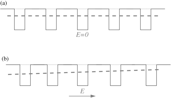
Figure 1: Simplified sketch of the planar-averaged electron potential energy, $-e\overline{V}(x)$ (black curves) for (a) an undistorted crystal, and (b) a crystal with a uniform longitudinal strain gradient. The red dashed lines show the macroscopic averages of the aforementioned functions.

As an illustration of the above derivations, it is useful in this context to work out a simple toy model that can be solved analytically; this will be also useful to point out some unconventional aspects of the flexoelectric response that have no counterpart in earlier theories of electromechanical effects in solids. We consider a rocksalt ionic crystal such as NaCl or MgO, and suppose that a longitudinal strain gradient develops along the (100) direction. Here we shall focus on electronic effects only, so that the atomic $x$ coordinates undergo displacements that are a predetermined quadratic function of $x$ with no further relaxations. For the time being we shall also assume that the crystal is perfectly ionic, i.e., that its electronic charge density can be approximated by a superposition of spherical closed-shell ions whose shape is not altered by changes in bond distances, etc. With the above assumptions in mind, one can perform an average of the electrostatic potential in the $yz$ planes, and express the result as a one-dimensional function of $x$. The atomic planes will appear as a periodic arrangement of potential wells (each well corresponding to a single charge-neutral monolayer), whose shape will reflect the radial distribution of electrons in the constituent ionic species. For the present purposes, the fine details of the potential wells are irrelevant; the only important quantity will be

$$K=-e\int_{-\infty}^{\infty}\overline{V}_{\textrm{ML}}(x)\,dx\,,$$ (54)

where $\overline{V}_{\textrm{ML}}(x)$ is the $yz$-averaged electric (Hartree) potential $V_{\textrm{ML}}({\bf r})$ generated by one monolayer, and $-e\overline{V}_{\textrm{ML}}(x)$ is the corresponding electron potential energy. Thus, for purposes of illustration we can represent the potential-energy wells as nonoverlapping rectangular dips of area $|K|$, whose shape is fixed and independent of the surrounding neighbors, as sketched in Fig. 1(a). As the wells are all identical and their separations are uniform in the undistorted crystal, the macroscopic electron potential energy obtained by convoluting the corresponding microscopic function with an appropriate low-pass filter [17], shown as a dashed line in Fig. 1(a), is constant. After freezing in the strain gradient deformation pattern, as shown in Fig. 1(b), the interlayer distance increases linearly along the chosen axis, leading to a constant slope in the macroscopic electrostatic potential and, hence, to a uniform electric field throughout the bulk crystal. This result points to a nonzero flexoelectric coefficient of purely electronic origin, since we explicitly neglected possible internal strains.

There are several important questions that naturally arise at this stage. The first obvious one is whether (and if yes, how) the outcome of Fig. 1 can be rationalized in the context of the theory developed in this Chapter. A second and less obvious issue arises in pseudopotential-based first-principles calculations, where one may wonder whether and how the results depend on choice of pseudopotential. The third question concerns the physical nature of the electric field that we describe in Fig. 1(b). Does it, for example, produce a direct force on charged particles such as electron and hole carriers and ionic cores?

To answer the first question, it suffices to suppose that the electrostatic potential wells are generated by a regular lattice of spherical charge distributions. To make things simple, consider a monatomic lattice, as for a rare-gas solid, that we construct by periodically repeating a spherical charge distribution $\rho_{0}({\bf r})$. We assume that the volume of the unit cell $\Omega({\bf r})$ depends smoothly on space as a result of an inhomogeneous macroscopic deformation. One can show (see Supplementary Note 1 of Ref. 15) that the resulting macroscopically averaged (in three dimensions) electric potential is given by

$$V({\bf r})=-\frac{1}{6\epsilon_{0}\Omega({\bf r})}\int d^{3}s\,s^{2}\rho_{0}(s)=-\frac{1}{6\epsilon_{0}\Omega({\bf r})}O_{\rm L},$$ (55)

where $O_{\rm L}=4\pi\int ds\,s^{4}\,\rho_{0}(s)$ is the isotropic quadrupole moment  of the static charge distribution $\rho_{0}({\bf r})$. Equivalently, it is the longitudinal component $O_{\rm L}=\sum_{\kappa}Q^{(3,xxx)}_{\kappa x}$ of the dynamical octupole tensor defined in Eq. (47), as follows from straightforward algebra.

In the linear regime (small deformations) we have

$$\Omega({\bf r})\simeq\Omega(1+\det{[\varepsilon({\bf r})]}),$$ (56)

which leads to the variation in the macroscopic electrostatic potential induced by the deformation,

$$\Delta V({\bf r})=\frac{1}{6\epsilon_{0}\Omega}\det{[\varepsilon({\bf r})]}O_{\rm L}$$ (57)

Assuming that the crystal has cubic symmetry and making use of Eq. (50), this yields, after some algebra, two of the three independent components of the flexoelectric tensor

$$\bar{\mu}^{\rm II}_{\alpha\alpha,\beta\beta}=\frac{O_{\rm L}}{6\Omega}.$$ (58)

(In the case of a biatomic ionic crystal one simply needs to replace $O_{\rm L}$ with the sublattice sum of the dynamical octupoles of the individual atoms.) By using the relationship between ${\bf J}$-tensors and ${\bf Q}$-tensors discussed earlier in this Section, it is not difficult to deduce that the third component, $\bar{\mu}^{\rm II}_{\alpha\beta,\alpha\beta}$ with $\alpha\neq\beta$, must be zero. Summarizing the above, the three independent components (longitudinal, transverse and shear) in a rigid-sphere crystal read as

$$\bar{\mu}^{\rm II}_{xx,xx}=\frac{O_{\rm L}}{6\Omega},\qquad\bar{\mu}^{\rm II}_{xx,yy}=\frac{O_{\rm L}}{6\Omega},\qquad\bar{\mu}^{\rm II}_{xy,xy}=0.$$ (59)

This demonstrates that the effect illustrated in Fig. 1 is indeed a natural consequence of the theory developed in this Chapter.

We now turn to the second question, concerning the use of pseudopotentials in first-principles calculations, as discussed in Ref. 12. One aspect of the pseudopotential approximation is the replacement of the all-electron charge density $\rho^{\rm AE}(r)$ by a pseudo charge density $\rho^{\rm PS}(r)$ in the core region of the atom. Since these charge densities are essentially rigid and spherically symmetric, the above considerations apply to them. As a result, to compensate for the use of the pseudopotential, one should add a “rigid core correction”

$$O_{{\rm L},\kappa}^{\rm RCC}=4\pi\int ds\;s^{4}\,\left[\rho_{\kappa}^{\rm AE}(r)-\rho_{\kappa}^{\rm PS}(r)\right]$$ (60)

to the longitudinal dynamic octopole of each atom $\kappa$ to recover the all-electron result. This propagates into a change $\Delta Q^{(3,xxx)}_{\kappa x}=3\Delta Q^{(3,xyy)}_{\kappa x}=O_{{\rm L},\kappa}^{\rm RCC}$, and to a change of $\bar{\mu}^{\rm II}_{xx,xx}$ and $\bar{\mu}^{\rm II}_{xx,yy}$ (but not $\bar{\mu}^{\rm II}_{xy,xy}$) by $\sum_{\kappa}O_{{\rm L},\kappa}^{\rm RCC}/6\Omega$. 

This rigid-core correction is not small, and is not independent of the details of pseudopotential construction. Therefore, two different calculations of the bulk flexoelectric response cannot be directly compared unless this correction has been applied in both cases. Nevertheless, as long as the same pseudopotential is consistently used in the calculation, predictions of physical, experimentally measurable quantities should not be affected by this correction. In particular, we shall see in Sec. (6) than $O_{{\rm L},\kappa}^{\rm RCC}$ makes an equal and opposite contribution to the surface contribution. Because of this cancellation, the total (bulk and surface) flexovoltage response [see Eq. (61)] can be computed without the need for including this correction.

The third question, regarding the physical nature of the resulting electric field, requires taking a closer look at some earlier works on the theory of absolute deformation potentials.[18, 19] (These can be regarded as the foundation of the modern theory of flexoelectricity, even if they were aimed at addressing a slightly different physical problem.) In a nutshell, if we wish to draw a band diagram of a crystal subjected to a strain-gradient deformation, knowledge of the macroscopic electrostatic field is not sufficient. Indeed, the relative location of the valence-band maximum or conduction-band minimum with respect to the electrostatic reference is itself a function of the local strain (via the so-called band-structure term), which implies that each band will “see” a different electric field. This means that one band edge may be perfectly flat, and the corresponding carriers feel no force whatsoever, even while the other band edge and/or the mean electrostatic potential can be strongly tilted.  In fact, even a metal subjected to a strain gradient will generally have a nonzero internal macroscopic electric field arising from a gradient in the mean electrostatic potential, although no current will flow. Thus, one should be careful not to interpret the macroscopic electric field produced by the flexoelectric effect in a longitudinal acoustic wave as a “real” physical field; it is just the tilt of some arbitrary reference energy that may have little to do with the phenomenon of interest in a given specific case. Just as for the notion of a “flexoelectric field,” care must be used when speaking of “short-circuit” and “open-circuit” electrical boundary conditions, as these are ambiguous in the nonperiodic strain-gradient world.

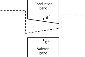
Figure 2: Sketch of valence bands (VB) and conduction bands (CB) for a slab with a strain gradient across its width. Dashed line indicates the macroscopic electron potential energy $V(x)=-e\phi(x)$. Hole carriers feel no force because the VB maximum is flat, while electron carriers feel a force to the right, both of which are contrary to naive expectations based on the electric field pointing to the right in the interior of the slab.

In light of the above arguments, it is legitimate to wonder whether the bulk flexoelectric effect is experimentally measurable at all. In fact, there are good reasons to believe that the tilt of the mean electrostatic potential does not provide a realistic description of the response – at least no more realistic than other reference energies (e.g., the conduction band bottom, or the valence band top, or the Fermi level). First, as we have argued above, the present theory yields a finite open-circuit “flexoelectric field” even in a metal, which is physically inconsistent. Second, if we go back to the example of the noninteracting spherical atoms, there are apparent inconsistencies as well: Since we have assumed that each potential well is independent of its environment, its motion cannot, in principle, be detected by an electrode that is placed at the far-away surface of the sample – and yet, the bulk flexoelectric coefficients do not vanish. We have, therefore, a sort of paradoxical situation, where the presence of a macroscopic electric field inside the material is indisputable, but at the same time there cannot be any open-circuit voltage, because of the hypothesis of rigid potential wells (which excludes long-range effects). To resolve these paradoxes, and place the present theory in the right context regarding experimental measurements, it is necessary to account for surface effects. We shall see how to do this in the following Sec. 6.

6 Surface effects

Knowing whether a given physical property is sensitive to the details of the sample surfaces is a matter of central importance in condensed matter theory. In the majority of cases (e.g., piezoelectricity), surfaces typically start to matter only at small length scales, where they are responsible for deviations in the measured property from the corresponding bulk value. There are situations, however, where such a sensitivity to the crystal termination persists up to the macroscopic scale; flexoelectricity belongs to this category. In the present Section we shall elaborate on this statement from a heuristic point of view, which is anyway sufficient to illustrate the most relevant physical ideas. A more formal discussion, based on a microscopic theory of the response to deformations, will be presented in Sec. 7 and Sec. 8.

In order to calculate the flexoelectric response of a finite object such as a slab it is appropriate to consider, rather than the induced macroscopic polarization, the open-circuit voltage $\Delta V$ produced by the deformation.  We shall only focus, in the following, on contributions that tend to a finite constant in the limit of infinite thickness $t$, and introduce the flexovoltage coefficient,

$$\varphi_{x\lambda,\beta\gamma}=\lim_{t\rightarrow\infty}\frac{1}{t}\frac{\partial\Delta V}{\partial\varepsilon_{\beta\gamma,\lambda}}.$$ (61)

Recall that $\varepsilon_{\beta\gamma,\lambda}=\partial\varepsilon_{\beta\gamma}/\partial r_{\lambda}$ is the gradient of the symmetric strain tensor along the Cartesian direction $r_{\lambda}$, and $x$ indicates the direction normal to the surface.  For simplicity, here we shall also restrict our analysis to strain gradients of the type $\varepsilon_{\alpha\alpha,x}$, i.e., a diagonal (either longitudinal or transverse) component of the symmetric strain tensor that is linearly growing across the slab thickness. (These are sufficient to describe the bending of a free-standing slab; a more general analysis, including the shear component, is deferred to Sec. 8.) We shall write the flexovoltage coefficient as a sum of bulk and surface-specific contributions,

$$\varphi_{xx,\alpha\alpha}=\varphi^{\rm bulk}_{xx,\alpha\alpha}+\varphi^{\rm surf}_{xx,\alpha\alpha},$$ (62)

whose explicit forms will be derived in the following paragraphs.

Electronic surface response

First let us consider only the purely electronic (frozen-ion) response. Strain gradients of the type $\varepsilon_{\alpha\alpha,x}$ are governed by Eq. (50); in our present notation this implies that the (open-circuit) uniform electric field that builds up in the interior of the slab as a consequence of the deformation is uniquely given in terms of the bulk flexoelectric coefficient of the material and its macroscopic dielectric constant by

$$\frac{\partial{E}^{\rm slab}_{x}}{\partial\varepsilon_{\alpha\alpha,x}}\Big{|}_{\rm frozen-ion}=-\frac{\bar{\mu}^{\rm II}_{xx,\alpha\alpha}}{\epsilon_{0}\bar{\epsilon}_{\rm r}}.$$ (63)

Here $\epsilon_{0}$ and $\epsilon_{\rm r}$ are the vacuum and relative permittivities, respectively, while $\mu^{\rm II}$ is the type-II flexoelectric tensor; as before, we use the bar symbol to distinguish frozen-ion quantities from fully relaxed ones. Since the electric field is minus the derivative of the potential, the bulk internal field contribution to the overall open-circuit voltage is then proportional to $t$, leading to a finite contribution to the overall flexovoltage coefficient that we identify with $\bar{\varphi}^{\rm bulk}$,

$$\bar{\varphi}^{\rm bulk}_{xx,\alpha\alpha}=-\frac{\partial{E}^{\rm slab}_{x}}{\partial\varepsilon_{\alpha\alpha,x}}\Big{|}_{\rm frozen-ion}=\frac{\bar{\mu}^{\rm II}_{xx,\alpha\alpha}}{\epsilon_{0}\bar{\epsilon}_{\rm r}}.$$ (64)

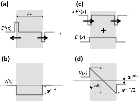
Figure 3: (a-b): Linear response of the electric field (a) and the electric potential (b) to a uniform strain applied to a film of thickness $t$. The function $E^{\rm U}$ (where U indicates “uniform”) can be regarded as representing a surface piezoelectric response (surface dipole layer appearing in response to strain). (c-d): Linear response of the field (c) and the potential (d) in the case of a strain gradient. The sketch shows the derivative with respect to $(\varepsilon_{\alpha\alpha,x}t)$ for a strain variation $\varepsilon_{\alpha\alpha}(x)=x\varepsilon_{\alpha\alpha,x}$ in a slab extending from $-t/2<x<t/2$. The field response contains two contributions. The first is given by $E^{\rm U}$, appropriately scaled by the linearly varying local strain. Note that the induced surface dipoles, schematically illustrated by arrows, now point in the same direction. The other is given by genuine strain-gradient effects contained in $E^{\rm G}$, which essentially reflects the bulk flexovoltage response. The resulting potential response in (d) thus consists in a macroscopic internal field plus a surface dipole contribution.

The surface contribution $\varphi^{\rm surf}$ in Eq. (62) originates from the fact that a surface can always be characterized by a potential offset $\phi$ between the macroscopic potential just inside and just outside the surface, and that this offset is different for the two surfaces in the presence of a strain gradient. Consider first the case of a uniform strain $\varepsilon_{\alpha\alpha}$ applied to a slab of thickness $t$, as shown in Fig. 3(a-b). The figure shows the derivative of the macroscopic electric field (panel a) and electron potential energy (panel b) with respect to the applied uniform strain $\varepsilon_{\alpha\alpha}$, and $\varphi^{\textrm{surf}}$ is the corresponding derivative of the potential offset $\phi$. The variation of $\phi$ with strain can be regarded as resulting from the fact that the surface, by virtue of its lack of inversion symmetry, is locally piezoelectric.  For the slab as a whole, however, a uniform strain does not produce a net voltage, since the induced potential offsets on either side of the slab cancel each other, consistent with the fact that the overall slab is nonpiezoelectric.

In the case of a strain-gradient deformation, on the other hand, the local strains at the opposite surfaces are opposite in sign, and do not cancel out, as illustrated in Fig. 3(c-d). The slab is taken to extend over $-t/2<x<t/2$ with local strain $\varepsilon_{\alpha\alpha}(x)=x\varepsilon_{\alpha\alpha,x}$, reaching values of $\varepsilon_{\alpha\alpha}=\pm(t/2)\varepsilon_{\alpha\alpha,x}$ at the two surfaces. The figure shows the derivative of the field (panel c) and potential (panel d) with respect to $(\varepsilon_{\alpha\alpha,x}t)$. This means that the induced potential offsets at the two opposite surfaces have the same sign and add up in a flexoelectric experiment, leading to a surface contribution of the form

$$\bar{\varphi}^{\rm surf}_{xx,\alpha\alpha}=\frac{\partial\phi}{\partial\varepsilon_{\alpha\alpha}}\Big{|}_{\rm frozen-ion}.$$ (65)

The total flexovoltage coefficient then reads as

$$\bar{\varphi}_{xx,\alpha\alpha}=\frac{\bar{\mu}^{\rm II}_{xx,\alpha\alpha}}{\epsilon_{0}\bar{\epsilon}_{\rm r}}+\bar{\varphi}^{\rm surf}_{xx,\alpha\alpha}.$$ (66)

The above derivation allows us to solve the paradoxes that we mentioned at the end of the previous Section. First, recall that we encountered some difficulties in giving a physical interpretation to the “internal electric field” that is induced by a strain gradient, as such a field depends on the reference energy (i.e., Bloch electrons in different eigenstates do not experience the same electrical force). This issue is easily solved by observing that the surface potential offset $\phi$ suffers from the same ambiguity as the bulk flexoelectric field; we defined it relative to the macroscopically averaged electrostatic potential under the surface, but we could have used the valence or conduction band edge instead. It is easy to see that the respective ambiguities contained in the surface and bulk terms exactly cancel, yielding an overall flexovoltage coefficient that is uniquely defined. Next, we have observed that there is an apparent physical inconsistency in the rigid-spherical-atom model, in that there should be no overall voltage response to a strain gradient, and yet the bulk flexoelectric coefficient does not vanish. It is easy to see that, once the surface contribution is taken into account, the total flexovoltage response of a slab made of noninteracting spherical atom is zero as it should be. Indeed, when such a slab is subjected to a uniform strain, its surface potential voltage response is

$$\bar{\varphi}^{\rm surf}_{xx,xx}=\bar{\varphi}^{\rm surf}_{xx,yy}=-\frac{O_{\rm L}}{6\epsilon_{0}\Omega}\,,$$ (67)

since a positive longitudinal or transverse strain increases the spacing between the atomic spheres and thereby reduces the surface potential offset. But, using Eqs. (58) and (64) (and the fact that $\bar{\epsilon}_{\rm r}=1$ for this model), this is exactly $-\bar{\varphi}^{\rm bulk}_{xx,\alpha\alpha}$, leading to the claimed cancellation in Eq. (66). This cancellation also explains why the replacement of the all-electron by the pseudo core charge density in the context of pseudopotential calculations has no effect on the total flexovoltage response, so that the rigid-core correction of Eq. (60) can be neglected, as was claimed in Sec. 5.

Note that the spherical atom model, in spite of its simplicity, is crucial to understand how flexoelectricity works in real materials. As we shall see in the results section, there generally tends to be a large cancellation between surface and bulk contributions to the flexoelectric effect. This happens because, even in covalently-bonded materials, the electronic charge distribution that is dragged along by each atom during its motion is largely constituted by a spherical shell, with comparatively smaller aspherical components. Spherical objects do not contribute to the overall flexovoltage coefficient of a slab, hence the aforementioned cancellation.

This gives a measure of the importance of the surface contribution – only when it is correctly taken into account together with the bulk term we obtain a meaningful physical quantity. Therefore, asking whether the surface contribution is “large or small” compared to the bulk effect is a poorly formulated question; the two must always go hand in hand. Instead, a more physically meaningful question is “How strong is the dependence of the surface contribution on its atomic and electronic structure?”

Based on these considerations, one can attempt to give an answer to a long-standing question that has been somewhat controversial in recent years: “Is flexoelectricity a bulk property?” As we said above, if by “flexoelectricity” we refer to the result of a typical flexoelectric experiment (i.e., where the induced current upon bending a short-circuited slab is measured), the answer is no. Conversely, if by the same name we call the current flowing through the bulk of the material while well-defined internal electrical boundary conditions are imposed, then the answer is yes. The problem is that the internal electrical boundary conditions depend on the externally-applied ones in a way that is surface-dependent, and unlike in the case of most known material properties, such a dependence persists in the limit of a macroscopically thick sample. All in all, in the present context we would rather stay away from the traditional rigid classification into bulk properties and surface properties, as flexoelectricity, strictly speaking, does not belong cleanly to either category.

Lattice surface response

We now discuss how the above conclusions need to be modified when full ionic relaxations are incorporated – these are, of course, of the utmost importance for a realistic description of the flexoelectric effect. Essentially, the above conclusion still hold, except for two important details: (i) the frozen-ion quantities (flexoelectric coefficient, dielectric constant, surface potential response) need to be replaced with their relaxed-ion counterparts; (ii) an effective deformation, given by an appropriate linear combination of, e.g., a longitudinal and transverse strain gradient, need to be considered in place of the individual tensor components.

To illustrate the implications of (i) and (ii) in a practical situation, it is useful to work out the explicit formulas for the simplest case of an unsupported slab subjected to bending.  Linear elasticity dictates that a transverse strain gradient (corresponding to a “frozen-ion” bending deformation) at static equilibrium must be accompanied by a longitudinal strain gradient, which for most materials will have opposite sign compared to the transverse one. In fact, the top layers of the slab (“top” here means furthest from the bending center) are under tensile strain, and this typically induces a longitudinal contraction of such layers, whose magnitude is related to the Poisson’s ratio of the material. Conversely, the bottom layers are transversely compressed, and will therefore expand longitudinally by an equal amount. This means that, to calculate the static flexovoltage coefficient of a bent slab, we need to consider the “effective” deformation

$$\varepsilon_{yy,x}=\varepsilon_{{\rm eff},x};\quad\varepsilon_{xx,x}=-\nu\varepsilon_{{\rm eff},x},$$ (68)

rather than the individual strain-gradient tensor components, where

$$\nu=\frac{\mathcal{C}_{xx,yy}}{\mathcal{C}_{xx,xx}}$$ (69)

is uniquely given by the elastic constants of the bulk material. Consequently, when the ions are relaxed, we shall be concerned with an effective flexovoltage coefficient reflecting the aforementioned mechanical equilibrium condition,

$$\varphi_{xx,{\rm eff}}=\frac{\mu^{\rm II}_{xx,{\rm eff}}}{\epsilon_{0}\epsilon_{\rm r}}+\frac{\partial\phi}{\partial\varepsilon_{\rm eff}},$$ (70)

where

$$\varepsilon_{yy}=\varepsilon_{{\rm eff}};\quad\varepsilon_{xx}=-\nu\varepsilon_{{\rm eff}}$$ (71)

refers to an analogous linear combination of the uniform strain components.

The fact that, even at the level of the surface contribution, we have an effective response to a combined transverse and longitudinal strain is fully consistent with the behavior of an unsupported slab subjected to uniform in-plane tension. In such a situation, the relaxation will affect not only the surface atoms, but will also extend to the entire slab, leading to a contraction in the third dimension proportional to the bulk coefficient $\nu$. Thus, for a free film in a relaxed-ion context, it is only meaningful to consider the response of the surface potential offset $\phi$ to $\varepsilon_{{\rm eff}}$, and not to the individual $\varepsilon_{yy}$ or $\varepsilon_{xx}$ components; the former is precisely the quantity that enters the total flexovoltage coefficient in Eq. (70).

Of course, one generally needs to consider more realistic mechanical boundary conditions than that of a free-standing film. In such cases, some of the specifics of the above example are no longer valid (e.g., the absence of surface loads). Still, the points (i) and (ii) are applicable to the most general case.

7 Electronic and lattice response revisited: Curvilinear coordinates

In the early Sections of this Chapter we have described a fundamental theory of the bulk flexoelectric effect, based on a first-principles quantum-mechanical description of the insulating crystal. Later, in Sec. 6 we have argued, based on heuristic arguments, that there are important surface contributions to the flexoelectric response of a finite sample, and that these need to be accounted for when discussing experimental results. Here, we shall put the derivations of Sec. 6 on firmer theoretical grounds by developing an alternative approach. In particular, we shall clarify how to describe the microscopic charge and current responses to an arbitrary inhomogeneous strain field in terms of cell-periodic response functions. Such a formalism is necessary in order to treat, in full generality, the response of a finite (and hence, spatially inhomogeneous) body to a deformation. As we shall see later, this will be useful not only for the formal derivation of the surface contributions to the flexoelectric effect in finite samples, but also for the practical calculation of the transverse bulk components of the flexoelectric tensor. (Recall that such components are presently difficult to access at the bulk level.) Given its rather technical character, and the fact that the most relevant physical results have already been presented in Section 6, this Section and the following can be skipped on a first reading.

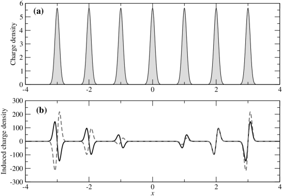
Figure 4: (a) Unperturbed charge density of model 1D crystal composed of Gaussian charge packets. (b) Change of charge density in linear response to a uniform strain (solid line) or strain gradient (dashed line).

A simple one-dimensional example

In order to establish a microscopic theory of deformations, the first issue one needs to address concerns the proper representation of the scalar and vector fields that describe the physical property of interest (e.g., atomic positions, electronic charge density, etc.). To appreciate the nature of the problem, it is useful to analyze the charge-density response of a simple lattice to a macroscopic deformation. Consider a one-dimensional chain of equally spaced atoms, which we represent as a regular array of Gaussian charge distributions as in Figure 4(a). Its unperturbed charge density is

$$\rho(x)=\sum_{n}\rho_{0}(x-R_{n}),\qquad\rho_{0}(x)=\frac{1}{\sigma\sqrt{\pi}}e^{-x^{2}/\sigma^{2}},$$ (72)

where $R_{n}=na$ is an integer multiple of the lattice parameter $a$. Now we apply a uniform expansion to the chain by displacing each atom by

$$u_{n}=\varepsilon R_{n},$$ (73)

and we look at how the charge density responds to such a perturbation . In the linear limit (small lambda) we obtain the response function $\partial\rho(x)/\partial\varepsilon$ that is plotted as the black curve in Fig. 4(b). The form of $\partial\rho(x)/\partial\varepsilon$ is manifestly problematic: such a function grows linearly when moving away from the origin, i.e., it is clearly nonperiodic, which contrasts with the fact the system remains periodic after the application of the perturbation. Moreover, it introduces an undesirable dependence of the result on the arbitrary location of the coordinate origin. Such issues become even more severe when considering a strain-gradient perturbation of the type

$$u_{n}=\frac{\eta}{2}R_{n}^{2}.$$ (74)

The charge density response, plotted as the red curve in Fig. 4(b), now grows quadratically with the value of the unperturbed atomic position, and extracting any relevant physical information from such a function appears difficult.

The solution of the above problems comes from the realization that the fixed laboratory frame is a poor choice of coordinate system if we wish to represent the response to a macroscopic elastic deformation. In such a frame, the boundary atoms in a large crystallite have to move very far from their original location even if the applied strain is small; if we naively take the difference in the charge density from the original to the current state we obtain a result that has little physical meaning, and most likely will strongly deviate from the linear regime that we have in mind. A viable alternative is to treat an elastic deformation as a deformation of space, rather than an atomic displacement pattern. This implies applying a coordinate transformation that exactly reproduces the macroscopic elastic deformation.  From this viewpoint, the atoms do not explicitly move from their original location, although they do move with respect to the laboratory frame because the coordinate system itself is changing.

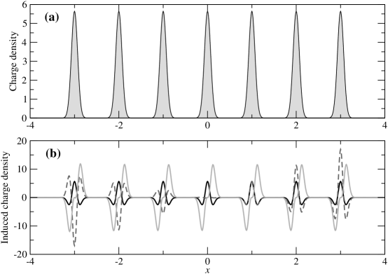
Figure 5: (a) Same as in Fig. 4(a). (b) Change in charge density, when expressed in transformed coordinates, for a uniform strain (solid black line) or a strain gradient (dashed dark gray line). The latter, while not periodic, can be expressed as a sum of black and light gray contributions (the latter was magnified by a factor of 50), as explained in the text.

To be explicit, consider a distortion ${\bf r}^{\prime}={\bf r}+{\bf u}({\bf r})$ that maps point $\bf r$ in the original periodic crystal into point ${\bf r}^{\prime}$ of the distorted crystal, and such that a nucleus at ${\bf R}_{l\kappa}$ would be carried to ${\bf R}^{\prime}_{l\kappa}={\bf R}_{l\kappa}+{\bf u}({\bf R}_{l\kappa})$ if one neglects the additional internal displacements arising from the lattice effects described in Sec. 4. If the initial charge density $\rho_{0}({\bf r})$ were also carried along by this distortion, the new charge density would be

$$\rho_{\textrm{ref}}({\bf r}^{\prime})=\rho_{0}({\bf r})\,{\rm det}^{-1}({\bf h})$$ (75)

where the Jacobian factor involving $h_{\alpha\beta}=\partial r^{\prime}_{\alpha}/\partial r_{\beta}=\delta_{\alpha\beta}+\partial u_{\alpha}/\partial r_{\beta}$ is needed to reflect the dilution or concentration of charge density. In fact, the actual charge density $\rho({\bf r}^{\prime})$ has to be computed from the appropriate physical laws (e.g., first-principles DFT calculations), so it will not be equal to $\rho_{\textrm{ref}}({\bf r}^{\prime})$. However, we may hope that the difference $\rho({\bf r}^{\prime})-\rho_{\textrm{ref}}({\bf r}^{\prime})$ is small, and we want to express this difference in terms of the original spatial variable $\bf r$. This is conveniently done by defining

$$\hat{\rho}({\bf r})=\rho({\bf r}^{\prime})\,\det({\bf h})$$ (76)

so that our small quantity is $\Delta\hat{\rho}({\bf r})=\hat{\rho}({\bf r})-\rho_{0}({\bf r})$. Note that $\hat{\rho}({\bf r})$ describes the actual charge density after the deformation, but transformed back to the original coordinate system; the hat symbol is used henceforth to highlight quantities that describe the transformed system from the curvilinear-coordinate point of view.

In Fig. 5 we again perform the same analysis as in Fig. 4, illustrating how the use of coordinate transformations effectively solves the problems that we pointed out earlier. Panel (a) shows the same charge density at rest. As before, in this model we assume that the actual charge densities shift rigidly with the nuclei. In panel (b) we plot as the black curve the induced density $\partial\hat{\rho}(x)/\partial\varepsilon$ for a uniform strain. The response is now periodic and much smaller in magnitude than before (note the scale change). We shall denote this response function as $\rho^{\rm U}(x)$, where ‘U’ indicates a ‘uniform’ strain. The response to a strain gradient, shown as the dashed red curve, is still not periodic, although it now has a milder dependence on the spatial coordinate, growing only linearly rather than quadratically with $x$. Remarkably, however, we can write this response as a linear combination of two cell-periodic functions,

$$\frac{\partial\hat{\rho}(x)}{\partial\eta}=x\rho^{\rm U}(x)+\rho^{\rm G}(x),$$ (77)

where $\rho^{\rm U}(x)$ is the same as above (response to uniform strain), and $\rho^{\rm G}(x)$ is a new quantity, reflecting the genuine strain-gradient effects (shown as a thick light gray curve in the figure, where it has been magnified by a factor of 50 to better illustrate its functional form). Since we are considering a uniform strain gradient above, we have $\varepsilon(x)=x\eta$, so that we can write

$$\Delta\hat{\rho}(x)=\varepsilon(x)\rho^{\rm U}(x)+\frac{d\varepsilon(x)}{dx}\rho^{\rm G}(x)+\ldots$$ (78)

In other words, we have achieved a closed expression for the induced charge density $\Delta\hat{\rho}(x)$ that depends only on proper measures of the local deformation, with the only hypothesis that the local strain $\varepsilon(x)$ varies slowly on the scale of the interatomic spacings.

Several questions naturally arise from the above discussion. First, how general is such an analysis? For our illustrative example above we have used a trivially simple system, and a single (longitudinal) strain (or strain gradient) type, so it is legitimate to wonder whether the same procedure is applicable to a full first-principles simulation in 3D. Second, what do we do with $\Delta\hat{\rho}(x)$ once we have calculated it? To make the discussion relevant for flexoelectricity it is necessary to trace a direct link between $\Delta\hat{\rho}(x)$ and measurable electrical quantities, such as the macroscopic polarization in short circuit, or the induced voltage in open circuit. We shall address both questions in the remainder of this Section.

General formalism in three dimensions

Regarding the general applicability of the coordinate transformation method, there are several conceivable ways to proceed. One could, for example, directly incorporate the curvilinear-coordinates formalism at the level of the Kohn-Sham equations (borrowing from the adaptive coordinate scheme of Gygi [20]) and, in a similar spirit as in Ref. 21, directly perform the perturbation expansion with respect to the metric tensor and its gradients. Alternatively – and we shall follow this latter strategy throughout this Chapter – one can go back to the phonon analysis that we have introduced in Sec. 2, this time focusing on the microscopic charge-density response functions; the challenge here lies in converting these to the curvilinear representation outlined in this Section. We thus consider a deformation

$$r^{\prime}_{\beta}({\bf r})=r_{\beta}+U_{\beta}e^{i{\bf q\cdot r}}$$ (79)

which generates a simple frozen phonon

$$u^{l}_{\kappa\beta}=U_{\beta}e^{i{\bf q\cdot R}_{l\kappa}}.$$ (80)

For the moment we neglect the internal displacements leading to the lattice response of Sec. 4, so that Eq. (80) is equivalent to Eqs. (9-10) with the $\bf q$-dependent terms neglected, but they will be restored shortly in Sec. 7.

In the linear limit, the charge density responds as

$$\rho({\bf r})=\rho_{0}({\bf r})+\rho^{\bf q}_{\beta}({\bf r})\,e^{i{\bf q\cdot r}}$$ (81)

where the cell-periodic part $\rho^{\bf q}_{\beta}({\bf r})$ gets modulated by the same phase factor as in Eq. (79). Inserting this in Eq. (76) gives

$$\hat{\rho}({\bf r})=\left(\rho_{0}({\bf r}^{\prime})+U_{\beta}\rho_{\beta}^{\bf q}({\bf r}^{\prime})e^{i{\bf q\cdot r}^{\prime}}\right)\,\left(1+iq_{\gamma}U_{\gamma}e^{i{\bf q\cdot r}^{\prime}}\right)$$ (82)

where the last term in parentheses is the value of $\det({\bf h})$ resulting from Eq. (79). We now expand the cell-periodic response function up to second order in ${\bf q}$,

$$\rho^{\bf q}_{\beta}({\bf r})=\rho^{(0)}_{\beta}({\bf r})-iq_{\gamma}\rho^{(1,\gamma)}_{\beta}({\bf r})-\frac{q_{\gamma}q_{\lambda}}{2}\rho^{(2,\gamma\lambda)}_{\beta}({\bf r}).$$ (83)

Since we are only collecting terms to first order in $\bf U$ in Eq. (82), we can ignore the distinction between $\bf r$ and $\bf r^{\prime}$ in the cross terms, but for the direct term we have

$$\rho_{0}({\bf r}^{\prime})=\rho_{0}({\bf r}+{\bf U}e^{i{\bf q\cdot r}})=\rho_{0}({\bf r})-U_{\beta}\rho_{\beta}^{(0)}({\bf r})e^{i{\bf q\cdot r}}$$ (84)

where we have used that $\partial_{\beta}\rho_{0}({\bf r})=-\rho_{\beta}^{(0)}({\bf r})$. Collecting all the terms linear in $\bf U$, we obtain

$$\Delta\hat{\rho}({\bf r})=U_{\beta}e^{i{\bf q\cdot r}}\left[iq_{\beta}\rho({\bf r})-iq_{\gamma}\rho^{(1,\gamma)}_{\beta}({\bf r})-\frac{q_{\gamma}q_{\lambda}}{2}\rho^{(2,\gamma\lambda)}_{\beta}({\bf r})\right].$$ (85)

The $\rho^{(0)}$ terms have now canceled, as expected from the fact that the coordinate transformation has removed the translational part from the response.

After observing that the unsymmetrized strain and strain gradient are related to partial derivatives of the displacement field,

$$\tilde{\varepsilon}_{\beta\gamma}({\bf r}) = iq_{\gamma}U_{\beta}e^{i{\bf q\cdot r}},$$ (86)

$$\eta_{\beta,\gamma\lambda}({\bf r}) = -q_{\gamma}q_{\lambda}U_{\beta}e^{i{\bf q\cdot r}},$$ (87)

we can readily write

$$\Delta\hat{\rho}({\bf r})=\tilde{\varepsilon}_{\beta\gamma}({\bf r})\left[\delta_{\beta\gamma}\rho({\bf r})-\rho^{(1,\gamma)}_{\beta}({\bf r})\right]+\frac{\eta_{\beta,\gamma\lambda}({\bf r})}{2}\rho^{(2,\gamma\lambda)}_{\beta}({\bf r}).$$ (88)

Finally, one can replace $\tilde{\varepsilon}_{\beta\gamma}$ with the symmetrized counterpart, $\varepsilon_{\beta\gamma}$ (the quantity in the square brackets is invariant upon $\beta\gamma$ exchange [13]), and replace $\eta_{\beta,\gamma\lambda}$ with the type-II strain gradient tensor $\varepsilon_{\beta\gamma,\lambda}$. This leads to an expression that is in all respects analogous to Eq. (78),

$$\Delta\hat{\rho}({\bf r})=\varepsilon_{\beta\gamma}({\bf r})\rho^{\rm U}_{\beta\gamma}({\bf r})+\frac{\partial\varepsilon_{\beta\gamma}({\bf r})}{\partial r_{\lambda}}\rho^{\rm G}_{\beta\gamma,\lambda}({\bf r}),$$ (89)

where the uniform (U) and gradient (G) terms are defined as follows,

$$\rho^{\rm U}_{\beta\gamma}({\bf r}) = \delta_{\beta\gamma}\rho({\bf r})-\rho^{(1,\gamma)}_{\beta}({\bf r}),$$ (90)

$$\rho^{\rm G}_{\beta\gamma,\lambda}({\bf r}) = \frac{1}{2}\left[\rho^{(2,\gamma\lambda)}_{\beta}({\bf r})+\rho^{(2,\lambda\beta)}_{\gamma}({\bf r})-\rho^{(2,\beta\gamma)}_{\lambda}({\bf r})\right].$$ (91)

This result formalizes and generalizes the arguments of the first part of this Section: it shows that the microscopic charge density response to an arbitrary inhomogeneous deformation can indeed be computed (and rigorously expressed in terms of well-defined response quantities) in a first-principles context, and for an arbitrary combination of the relevant 3D deformation tensor components.

As a side note, one can show that the quantity $\rho^{\rm U}_{\beta\gamma}({\bf r})$ essentially coincides (apart from a trivial scaling factor) with the first-order charge-density as defined by Hamann, Wu, Rabe and Vanderbilt [21] within their linear-response theory of strain based on the metric tensor. It will be interesting in the near future to draw even closer connections between the two formalisms, which bear several similarities at the conceptual level.

Microscopic polarization response

In the above derivations we have focused on the charge-density response of the system to an inhomogeneous deformation, but we could have worked just as well with the microscopic polarization response instead. This quantity is well-defined only for infinitesimal transformations, otherwise it depends on the specific path followed by the system during its evolution; this is not an issue here, since we are exclusively interested in the linear-response regime. The microscopic polarization ${\bf P}({\bf r})$ is related to the adiabatic current-density response of the system to a time-dependent perturbation. Thus, in order to construct an appropriate definition of this quantity in a generic curvilinear frame, we need first to examine the transformation laws of the current-density field ${\bf J}({\bf r})$. To this end, let ${\bf r}^{\prime}={\bf r}+{\bf u}({\bf r},t)$ be a generic time-dependent coordinate transformation, which we suppose to coincide, as usual, with the displacement field associated with the mechanical deformation of the sample. (We suppose now that such a deformation happens slowly over a finite interval of time.) In a curvilinear framework the four-current, defined as $J^{\mu}=(\rho,j_{1},j_{2},j_{3})$, transforms as

$$\bar{J}^{\mu}=\frac{\partial\bar{x}^{\mu}}{\partial x^{\alpha}}\,J^{\alpha}\,{\rm det}^{-1}\left[\frac{\partial\bar{x}^{\beta}}{\partial x^{\gamma}}\right],$$ (92)

where $x^{\mu}=(t,x_{1},x_{2},x_{3})$ is the coordinate four-vector and the barred (unbarred) symbols refer to the deformed (original) frame. We work here in the nonrelativistic limit with $\bar{t}=t$ and $\bf r$ independent of $t$, so that

$$\bar{\rho} = \rho\,{\rm det}^{-1}({\bf h}),$$ (93)

$$\bar{J}_{i} = \left(\rho\frac{\partial{u}_{i}}{\partial t}+h_{ij}J_{j}\right)\,{\rm det}^{-1}({\bf h}).$$ (94)

(Latin indices refer to the three-dimensional Cartesian space.) This leads to the definitions

$$\hat{\rho} = \bar{\rho}\,\det({\bf h}),$$ (95)

$$\hat{J}_{i} = ({\bf h}^{-1})_{ij}\left[\bar{J}_{j}-\bar{\rho}\frac{\partial{u}_{j}}{\partial t}\right]\det({\bf h}).$$ (96)

The above expression for the curvilinear-frame charge density $\hat{\rho}$ coincides with that postulated earlier in Eq. (76), showing that this definition is, in fact, dictated by the fundamental transformation laws of a scalar density field. Equation (96), on the other hand, gives the desired expression for the curvilinear-frame current density $\hat{J}_{i}$, which we will use in the following to derive the microscopic polarization response to an acoustic phonon perturbation.

As in the former case of the charge density response, we consider a monochromatic acoustic phonon as in Eq. (79), again without internal cell relaxations. This time, however, we allow the amplitude of the displacement to depend on time,

$${\bf r}^{\prime}={\bf r}+{\bf u}({\bf r},t),\qquad u_{\beta}({\bf r},t)=U_{\beta}(t)\,e^{i{\bf q\cdot r}}.$$ (97)

(Henceforth we shall go back to using Greek indices for three-dimensional space coordinates, as we did in the previous sections.) In the adiabatic limit, one has

$${\bf J}({\bf r},t)=\dot{U}_{\beta}(t)\frac{\partial{\bf P}({\bf r})}{\partial U_{\beta}},$$

and, after dropping all terms that are quadratic in either $U_{\beta}$ or $\dot{U}_{\beta}$ [this implies setting $h_{ij}=\delta_{ij}$ in Eq. (96)],

$$\hat{\bf J}({\bf r},t)=\dot{U}_{\beta}(t)\frac{\partial{\bf P}({\bf r})}{\partial U_{\beta}}-\dot{\bf U}(t)\rho_{0}({\bf r}).$$

Now, the microscopic polarization response can be written, as usual, as a cell-periodic part times a phase, ${\bf P}({\bf r})=U_{\beta}\,e^{i{\bf q\cdot r}}\,{\bf P}^{\bf q}_{\beta}({\bf r})$, which immediately leads to

$$\hat{P}_{\alpha}({\bf r})=U_{\beta}e^{i{\bf q\cdot r}}\left[{P}^{\bf q}_{\alpha,\beta}({\bf r})-\delta_{\alpha\beta}\rho_{0}({\bf r})\right].$$ (98)

By following the same steps as for the case of the charge-density response, we now proceed to expand ${P}^{\bf q}_{\alpha,\beta}({\bf r})$ in powers of ${\bf q}$,

$${\bf P}^{\bf q}_{\beta}({\bf r})={\bf P}^{(0)}_{\beta}({\bf r})-iq_{\gamma}{\bf P}^{(1,\gamma)}_{\beta}({\bf r})-\frac{q_{\gamma}q_{\lambda}}{2}{\bf P}^{(2,\gamma\lambda)}_{\beta}({\bf r}).$$ (99)

From translational invariance, it is then easy to show that the zeroth-order term

$$P^{(0)}_{\alpha,\beta}({\bf r})=\delta_{\alpha\beta}\rho_{0}({\bf r}),$$ (100)

exactly cancels with the last term involving $\rho_{0}$ in Eq. (98). Eventually, we arrive at a provisional result for the linearly induced polarization currents in the curvilinear frame of the deformed body in the form

$$\Delta\hat{P}_{\alpha}=\varepsilon_{\beta\gamma}({\bf r})P^{\rm U}_{\alpha,\beta\gamma}({\bf r})+\frac{\partial\varepsilon_{\beta\gamma}({\bf r})}{\partial r_{\lambda}}P^{\rm G}_{\alpha\lambda,\beta\gamma}({\bf r}),$$ (101)

where the cell-periodic vector fields ${\bf P}^{\rm U,G}$ are

$$P^{\rm U}_{\alpha,\beta\gamma}({\bf r}) = -P^{(1,\gamma)}_{\alpha,\beta}({\bf r}),$$ (102)

$$P^{\rm G}_{\alpha\lambda,\beta\gamma}({\bf r}) = \frac{1}{2}\left[P^{(2,\gamma\lambda)}_{\alpha,\beta}({\bf r})+P^{(2,\lambda\beta)}_{\alpha,\gamma}({\bf r})-P^{(2,\beta\gamma)}_{\alpha,\lambda}({\bf r})\right].$$ (103)

To arrive at this equation, however, we have had to assume that the currents generated by a global rotation are the same as those obtained by rigidly rotating a classical charge density that is equal to the true quantum-mechanical one. This assumption, which is implicit in Eq. (50), was used to conclude that $P^{(1,\beta)}_{\alpha,\gamma}({\bf r})=P^{(1,\gamma)}_{\alpha,\beta}({\bf r})$, and hence to replace the unsymmetrized ($\tilde{\varepsilon}$) with the symmetrized ($\varepsilon$) strain tensor (see Sec. V.C of Ref. 13). While such an assumption was indeed valid in the charge-density case, it is not obvious that it is justifiable in the present case of the microscopic polarization current. Discussing this point in detail would take us far from the scope of the present Chapter; nevertheless, the reader is warned that there are still some unresolved formal issues in the theory of the current-density response.

Regardless of such issues, one can show that the functions $\Delta\hat{\rho}$ and $\Delta\hat{\bf P}$ enjoy the fundamental relationship

$$\hat{\nabla}\cdot\Delta\hat{\bf P}({\bf r})=-\Delta\hat{\rho}({\bf r}),$$ (104)

where $\hat{\nabla}\cdot\hat{\bf A}$ indicates the divergence of the vector field $\hat{\bf A}$ in the curvilinear frame. (The hat is used to emphasize that the differentiation is with respect to ${\bf r}$ rather than ${\bf r}^{\prime}$.) This reflects a well-known fact, which is important in the specific context of flexoelectricity: the induced charge density can be readily deduced from the polarization, but not the other way around. As a matter of fact, taking the divergence annihilates the solenoidal part of the $\Delta\hat{\bf P}$-field, which does contribute to the bulk flexoelectric tensor. (Recall the relationship between dynamical octupoles and second moments of the current-density response: the additional information contained in the latter can indeed be ascribed to divergenceless polarization currents that arise in response to an atomic displacement.)

Atomic relaxations

We now return to the inclusion of the internal atomic relaxations, and describe how they can be conveniently incorporated in the aforementioned theory; the practical implications regarding surface effects will be discussed in Sec. 8.

The first important observation is that, given a strain field $\varepsilon_{\beta\gamma}({\bf r},t)$ that depends slowly on space and time, the internal-strain tensors that were introduced in Section 2 can readily be identified with the microscopic lattice response of the crystal in the curvilinear frame of the deformed body,

$$u^{l}_{\kappa\alpha}(t)=\varepsilon_{\beta\gamma}({\bf R}_{l\kappa},t)\Gamma^{\kappa}_{\alpha\beta\gamma}+\frac{\partial\varepsilon_{\beta\gamma}({\bf R}_{l\kappa},t)}{\partial r_{\lambda}}L^{\kappa}_{\alpha\lambda,\beta\gamma}+\ldots$$ (105)

In particular, for a macroscopic strain gradient, the above relationship reduces to

$$\frac{\partial u^{l}_{\kappa\alpha}}{\partial\varepsilon_{\beta\gamma,\lambda}}=R_{l\kappa\lambda}\,\Gamma^{\kappa}_{\alpha\beta\gamma}+L^{\kappa}_{\alpha\lambda,\beta\gamma}.$$ (106)

Next, it is easy to show that Eq. (101) still holds, provided that we replace the purely electronic response functions with their relaxed-ion counterparts,

$$P_{\alpha,\beta\gamma}^{\rm U}(x)\, = \,\bar{P}_{\alpha,\beta\gamma}^{\rm U}(x)+P_{\alpha,\kappa\rho}^{(0)}(x)\Gamma^{\kappa}_{\rho\beta\gamma},$$ (107)

$$P_{\alpha\lambda,\beta\gamma}^{\rm G}(x)\, = \,\bar{P}_{\alpha\lambda,\beta\gamma}^{\rm G}(x)-P_{\alpha,\kappa\rho}^{(1,\lambda)}(x)\Gamma^{\kappa}_{\rho\beta\gamma}+P_{\alpha,\kappa\rho}^{(0)}(x)L^{\kappa}_{\rho\lambda,\beta\gamma}.$$ (108)

(We have used the bar symbol here to denote the purely electronic $P^{\rm U,G}$ response functions and thereby distinguish them from the fully relaxed quantities.) This formally extends the microscopic linear-response theory discussed in this Section to the relaxed-ion case.

Electrostatics in a curved space

Having established a convenient form for the microscopic charge and polarization response functions, we still need to figure out how to use them, e.g., how to calculate the voltage response $V({\bf r})$. This requires some attention, given the fact that we are no longer working in the Cartesian frame of the laboratory. In particular, one needs to replace Gauss’s law with its “curvilinear” generalization[22, 23]

$$\hat{\nabla}\cdot(\hat{\bm{\epsilon}}\cdot\hat{\bf E})=\hat{\rho},$$ (109)

where the vacuum permittivity has been replaced with the tensor

$$\hat{\bm{\epsilon}}=\epsilon_{0}\det{({\bf h})}{\bf g}^{-1},$$ (110)

the hat on $\hat{\nabla}$ is again a reminder that the gradient is in the curvilinear frame, ${\bf g}={\bf h\cdot h}^{\rm T}$ is the metric of the deformation, and

$$\hat{E}_{\alpha}({\bf r})=h_{\alpha\beta}E_{\beta}({\bf r}^{\prime})$$ (111)

is the transformed electric field.  As $\hat{\nabla}V({\bf r})=-\hat{\bf E}({\bf r})$, the above strategy allows one to compute the induced electrostatic potential from the induced polarization (or charge density).  

In the linear limit of small deformations, one has

$$\epsilon_{0}\hat{\nabla}\cdot(\Delta\hat{\bf E}+\Delta{\bf E}^{\rm met})=\Delta\hat{\rho}({\bf r})$$ (112)

where $\Delta\hat{\bf E}({\bf r})=-\hat{\nabla}[\Delta V({\bf r})]$ is minus the (curvilinear) gradient of the induced electrostatic potential, $\Delta V$, and $\Delta{\bf E}^{\rm met}$, coming from the linearization of $\hat{\bm{\epsilon}}$, reads as

$$\Delta{E}^{\rm met}_{\alpha}({\bf r})=\varepsilon_{\beta\gamma}({\bf r})\left[\delta_{\beta\gamma}{E}_{\alpha}({\bf r})-\delta_{\alpha\beta}{E}_{\gamma}({\bf r})-\delta_{\gamma\alpha}{E}_{\beta}({\bf r})\right],$$ (113)

where ${E}_{\gamma}({\bf r})$ is the electric field in the unperturbed system. The choice of notation $\Delta{\bf E}^{\rm met}$ is meant to suggest a “metric contribution to the curvilinear-frame electric field,” but this is somewhat problematic as it is not an irrotational field. Alternatively, $\epsilon_{0}\Delta{\bf E}^{\rm met}$ could be regarded as a “metric contribution” to the polarization, since one can rewrite Eq. (112) in terms of $\Delta{\bf P}$ as

$$\epsilon_{0}\hat{\nabla}\cdot\Delta\hat{\bf E}=-\hat{\nabla}\cdot\left(\Delta{\bf P}+\epsilon_{0}\Delta{\bf E}^{\rm met}\right).$$ (114)

However, this is not entirely satisfactory either, as $\Delta{\bf E}^{\rm met}$ does not really originate from the displacement of charged particles. It is probably most appropriate to interpret $\epsilon_{0}\Delta{\bf E}^{\rm met}$ as a displacement current arising from the effective change of permittivity associated with the deformation of the reference frame.

In any case, Eq. (112) shows that the induced potential $\Delta V({\bf r})$ contains, in addition to contributions from the rearrangement of the electron cloud occurring during the deformation (these are contained in $\Delta\hat{\rho}$), also a term that depends on the local variation of the metric at fixed charge density. We shall come back to this point in the discussion of surface contributions to the flexoelectric effect in Section 8. Note that, by construction, the microscopic electric field response to an arbitrary deformation enjoys an analogous representation as the charge density response,

$$\Delta\hat{{E}}_{\alpha}({\bf r})=\varepsilon_{\beta\gamma}({\bf r}){E}^{\rm U}_{\alpha,\beta\gamma}({\bf r})+\frac{\partial\varepsilon_{\beta\gamma}({\bf r})}{\partial r_{\lambda}}{E}^{\rm G}_{\alpha\lambda,\beta\gamma}({\bf r}),$$ (115)

where both ${E}^{\rm U}$ and ${E}^{\rm G}$ are lattice-periodic functions whose explicit expressions can be readily derived from Eq. (112).

Treatment of the macroscopic electric fields

Eq. (112) specifies $\Delta\hat{\bf E}({\bf r})$ modulo an ${\bf r}$-independent integration constant, $\Delta\hat{\overline{\bf E}}$ whose value is fixed by the electrical boundary conditions (EBC) of the problem. The electronic response functions are typically defined (and calculated) by assuming $\Delta\hat{\overline{\bf E}}=0$, i.e., short-circuit (SC) EBCs, but any other EBC choice can be recovered if the charge-density (and/or polarization) response to a macroscopic electric field is known.  For example, in the case of the polarization one can write

$$\Delta\hat{P}_{\alpha}({\bf r}) =\Delta\hat{P}_{\alpha}^{\rm SC}({\bf r})+\Delta\hat{\overline{{E}}}_{\beta}P_{\alpha}^{{E}_{\beta}}({\bf r}),$$ (116)

where $P_{\alpha}^{{E}_{\beta}}({\bf r})=\partial P_{\alpha}({\bf r})/\partial{E}_{\beta}$ is the microscopic $P$ response to an applied field along $\beta$. [25] The contribution of the macroscopic field can be readily incorporated into the strain-gradient term (${\bf P}^{\rm G}$ in this case), as the macroscopic electric field response in a nonpiezoelectric crystal vanishes at the uniform-strain level. Therefore Eqs. (89), (101), and (115) remain valid in arbitrary EBC.

8 Surface effects in curvilinear coordinates

Recall that, in order to quantify the flexoelectric response of a free-standing slab, we have introduced the flexovoltage coefficient $\varphi_{x\lambda,\beta\gamma}$. Here we shall demonstrate how this quantity can be rigorously derived in the context of the microscopic theory developed in the previous Section. To express $\varphi_{x\lambda,\beta\gamma}$ in terms of well-defined response functions of the system, we shall follow the strategy of Sec. 7, now specializing to the case of a supercell geometry. As before, we shall derive the microscopic response of the system (charge density, polarization, and atomic displacements) to a strain-gradient deformation via a long-wave analysis of its acoustic phonons. With the help of a coordinate transformation to the curvilinear frame of the perturbed body, one can express such microscopic response functions in terms of “proper” measures of the local deformation, i.e., in a translationally and rotationally invariant form,

$$\Delta\hat{f}({\bf r})=\varepsilon_{\beta\gamma}({\bf r})f_{\beta\gamma}^{\rm U}({\bf r})+\frac{\partial\varepsilon_{\beta\gamma}({\bf r})}{\partial r_{\lambda}}f_{\beta\gamma,\lambda}^{\rm G}({\bf r})+\ldots$$ (117)

Here $\hat{f}$ can stand for the charge density ($\hat{\rho}$), polarization ($\hat{\bf P}$) or electric field ($\hat{\bf E}$) expressed in the curvilinear frame. Note that the cell-periodic functions $f^{\rm U}$ and $f^{\rm G}$, referring respectively to uniform and gradient terms, are characterized by an oscillatory behavior on the scale of an interatomic distance, due to the discreteness of the atomic lattice. As it is customary in the space-resolved analysis of many other physical properties (e.g., dielectric response), we shall assume in the following (unless otherwise specified) that such oscillations have been filtered out by means of an appropriate nanosmoothing [17, 26] technique.

Surface polarization and metric

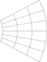
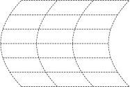
(a)	(b)	(c)

Figure 6: Schematic representation of the three types of strain gradient described in the text. (a) Longitudinal, $\varepsilon_{xx,x}$. (b) Transverse, $\varepsilon_{yy,x}$. (c) Shear, $\varepsilon_{xy,y}$. The $x$ and $y$ axes correspond to the horizontal and vertical directions in the figure respectively. (Adapted from Ref. 27.)

To illustrate the above arguments in the present context, consider a symmetrically terminated slab of a cubic material (we assume that the surfaces are parallel to the $yz$ plane), and perturb it with a strain-gradient deformation. We assume for the moment that the ionic coordinates simply follow the deformation; we shall lift this limitation in the next subsection. In order to calculate the flexovoltage coefficient of the slab, we shall first derive the electric field ${\bf E}({\bf r})$ induced by the deformation under open-circuit electrical boundary conditions. Then, by performing a line integral of ${\bf E}({\bf r})$ across the slab thickness, one can readily obtain the desired value of $\varphi_{\alpha\lambda,\beta\gamma}$. To calculate ${\bf E}({\bf r})$ we need, in turn, two basic ingredients: the microscopic polarization response, $\Delta{\bf P}({\bf r})$, and the “metric” contribution to the polarization, $\Delta{\bf E}^{\rm met}$. Regarding the former, after nanosmoothing ${\bf P}^{\rm U,G}$ are functions of $x$ only, and we can write

$$\frac{\partial\hat{P}_{\alpha}(\bf r)}{\partial\varepsilon_{\beta\gamma,\lambda}}\Big{|}_{\rm frozen-ion}=r_{\lambda}\bar{P}^{\rm U}_{\alpha,\beta\gamma}(x)+\bar{P}^{\rm G}_{\alpha\lambda,\beta\gamma}(x).$$ (118)

The two response functions $P^{\rm U}_{\alpha,\beta\gamma}(x)$ and $P^{\rm G}_{\alpha\lambda,\beta\gamma}(x)$ have the physical meaning of a local piezoelectric and flexoelectric coefficient, respectively. Note that $P^{\rm U}_{\alpha,\beta\gamma}(x)$ differs from zero only in the vicinity of the surface, as the bulk material is nonpiezoelectric. The metric term, on the other hand, reads as

$$\frac{\partial{E}^{\rm met}_{\alpha}({\bf r})}{\partial\varepsilon_{\beta\gamma,\lambda}}=r_{\lambda}\left[\delta_{\beta\gamma}{E}_{\alpha}(x)-\delta_{\alpha\beta}{E}_{\gamma}(x)-\delta_{\gamma\alpha}{E}_{\beta}(x)\right].$$ (119)

This quantity, just like ${\bf P}^{\rm U}$, is active only at the surface: the electric field of the undistorted slab is nonzero (and directed perpendicular to the surface plane) only in a small region where the crystal lattice is perturbed by the truncation of the bonding network.

The details of the derivation differ, from now on, depending on the specific type of flexovoltage response that one wishes to calculate. It can be shown that, given the symmetry of the slab, there are only three types of strain-gradient deformation that yield a net open-circuit voltage in a cubic material: a variation of $\varepsilon_{xx}$ with $x$ (longitudinal), $\varepsilon_{yy}$ with $x$ (transverse), or $\varepsilon_{xy}$ with $y$ (shear), which are responsible for the flexovoltages $\varphi_{xx,xx}$, $\varphi_{xx,yy}$, and $\varphi_{xy,xy}$ respectively, in the notation of Eq. (61).

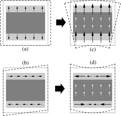
Figure 7: Schematic representation of the polarization fields induced by different macroscopic deformations of a slab of thickness $t$, drawn in the undistorted reference frame. The $x$ coordinate is vertical here. Left panels (a-b) illustrate uniform strains; right panels (c-d) refer to uniform strain gradients. Top (a,c) are transverse deformations (the situation is qualitatively identical in the longitudinal case, not shown), bottom (b,d) are shear patterns. The surface region and corresponding polarization field are indicated by light gray shading and black arrows. White arrows on a dark gray background refer to the bulk region. The dashed black frames indicate the type of deformation in each case. (Adapted from Ref. 15.)

Longitudinal and transverse cases. In these two cases (which we shall indicate as $xx,\alpha\alpha$), the system remains periodic in-plane, and the problem becomes essentially one-dimensional. We have, in particular,

$$\frac{\partial\hat{P}_{x}(x)}{\partial\varepsilon_{\alpha\alpha,x}}\Big{|}_{\rm FI} = x\bar{P}^{\rm U}_{x,\alpha\alpha}(x)+\bar{P}^{\rm G}_{xx,\alpha\alpha}(x),$$ (120)

$$\frac{\partial{E}^{\rm met}_{x}(x)}{\partial\varepsilon_{\alpha\alpha,x}} = x{E}_{x}(x)(1-2\delta_{\alpha x})$$ (121)

(where FI is shorthand for ‘frozen-ion.’) The polarization response functions $P^{\rm U}$ and $xP^{\rm U}+P^{\rm G}$ are schematically illustrated for the transverse case in Figs. 7(a) and (c) respectively. Given that both vector fields are irrotational and vanish at infinity, one can safely simplify Eq. (114) by removing the divergence sign on both sides to get

$$\frac{\partial\hat{E}_{x}(x)}{\partial\varepsilon_{\alpha\alpha,x}}\Big{|}_{\rm FI}=-\frac{1}{\epsilon_{0}}\left[x\bar{P}^{\rm U}_{x,\alpha\alpha}(x)+\bar{P}^{\rm G}_{xx,\alpha\alpha}(x)\right]-x{E}_{x}(x)(1-2\delta_{\alpha x}).$$ (122)

The frozen-ion flexovoltage coefficient of Eq. (61) can then be calculated by writing the open-circuit potential associated with the above field as

$$\Delta V=-\int_{-\infty}^{+\infty}dx\,\left[xE^{\rm U}_{x,\alpha\alpha}(x)+E^{\rm G}_{xx,\alpha\alpha}(x)\right],$$ (123)

where

$$E^{\rm U}_{x,\alpha\alpha}(x) = -\frac{1}{\epsilon_{0}}\bar{P}^{\rm U}_{x,\alpha\alpha}(x)-{E}_{x}(x)(1-2\delta_{\alpha x}),$$ (124)

$$E^{\rm G}_{xx,\alpha\alpha}(x) = -\frac{1}{\epsilon_{0}}\bar{P}^{\rm G}_{xx,\alpha\alpha}(x).$$ (125)

The above functions enjoy a number of useful properties:

1. $E^{\rm U}_{x,\alpha\alpha}(x)$ vanishes everywhere except for a small region near the surface at $x\sim\pm t/2$;

2. $E^{\rm U}_{x,\alpha\alpha}(x-t/2)=-E^{\rm U}_{x,\alpha\alpha}(-x+t/2)$ is antisymmetric, and independent of $t$ for a sufficiently thick slab;

3. $E^{\rm G}_{xx,\alpha\alpha}(x)$ corresponds to minus the bulk flexocoupling coefficient in the slab interior,

   $$E^{\rm G}_{xx,\alpha\alpha}(x\sim 0)=-\bar{\varphi}^{\rm bulk}_{xx,\alpha\alpha}=-\frac{\mu^{\rm bulk}_{xx,\alpha\alpha}}{\epsilon_{0}\bar{\epsilon}_{\rm r}},$$

   and only deviates from this value in a small region near the surface;

4. $E^{\rm G}_{xx,\alpha\alpha}(x-t/2)=E^{\rm G}_{xx,\alpha\alpha}(-x+t/2)$ is symmetric, and again independent of $t$ for a sufficiently thick slab.

Based on these observations, in the limit of large slab thickness one can approximate Eq. (123) as

$$\Delta V\sim-t\int_{0}^{+\infty}dx\,E^{\rm U}_{x,\alpha\alpha}(x)+t\bar{\varphi}^{\rm bulk}_{xx,\alpha\alpha}.$$ (126)

(We assume that $x=0$ is the center of the slab and $x=+\infty$ is deep in the vacuum region.) As the integral in the last equation is independent of $t$, we can readily write

$$\bar{\varphi}_{xx,\alpha\alpha}=-\int_{0}^{+\infty}dx\,E^{\rm U}_{x,\alpha\alpha}(x)+\bar{\varphi}^{\rm bulk}_{xx,\alpha\alpha},$$ (127)

whence we obtain

$$\bar{\varphi}^{\rm surf}_{xx,\alpha\alpha}=-\int_{0}^{+\infty}dx\,E^{\rm U}_{x,\alpha\alpha}(x).$$ (128)

The last equation states that the surface contribution to the flexovoltage response of a slab corresponds to minus the line integral of the induced electric field upon application of a uniform strain. The latter is, of course, the electrostatic potential offset response to uniform strain, $\partial\phi/\partial\varepsilon_{\alpha\alpha}$, that we already discussed in Sec. 6. We have, therefore, rigorously demonstrated that the flexovoltage response of the slab indeed contains both bulk and surface contributions, and that their nature is correctly described by Eq. (66). Note that the derivations presented here, in addition to corroborating the arguments of Sec. 6, allow us to make one step further and split $\bar{\varphi}^{\rm surf}_{xx,\alpha\alpha}$ into a polarization current and a metric term,

$$\frac{\partial\phi}{\partial\varepsilon_{\alpha\alpha}}=\frac{1}{\epsilon_{0}}\int_{0}^{+\infty}dx\,P^{\rm U}_{x,\alpha\alpha}(x)+(2\delta_{\alpha x}-1)\phi_{0}.$$ (129)

In the last term on the right, $\phi_{0}=-\int_{0}^{+\infty}dx\,{E}_{x}(x)$ is the potential offset before the perturbation.

In summary, in the present case (longitudinal or transverse strain gradient) the induced electric field in the interior of the film is a bulk property of the material – it is given by the flexoelectric coefficient divided by the macroscopic dielectric constant. The surface contribution, on the other hand, acts as an induced potential offset that grows linearly with slab thickness, and therefore scales similarly to the bulk contribution, as illustrated in Fig. 3.

Shear case. The case of a shear deformation ($xy,xy$) is qualitatively different from the former two cases.  Here we have

$$\frac{\partial\hat{P}_{\alpha}({\bf r})}{\partial\varepsilon_{xy,y}}\Big{|}_{\rm FI} = \delta_{\alpha y}yP^{\rm U}_{y,xy}(x)+P^{\rm G}_{\alpha y,xy}(x),$$ (130)

$$\frac{\partial{E}^{\rm met}_{\alpha}({\bf r})}{\partial\varepsilon_{xy,y}} = -\delta_{\alpha y}y{E}_{x}(x).$$ (131)

Figures 7(b) and (d) illustrate the polarization fields that are linearly induced by shear deformations. By taking the divergence of the above vector fields, we can write the curvilinear Poisson’s equation, Eq. (114), as a function of $x$ only, 

$$\epsilon_{0}\frac{\partial\hat{{E}}_{xy,xy}(x)}{\partial x}=-\bar{P}^{\rm U}_{y,xy}(x)-\frac{\partial\bar{P}^{\rm G}_{xy,xy}(x)}{\partial x}+\epsilon_{0}{E}_{x}(x).$$ (132)

[We have used the short-hand notation $\hat{E}_{xy,xy}(x)=\partial\hat{E}_{x}(x)/\partial\varepsilon_{xy,y}$.] Assuming that the field vanishes inside the slab,  we can then calculate the macroscopic electric field in the vacuum region,

$$\epsilon_{0}\frac{\partial\hat{E}_{x}(x=+\infty)}{\partial\varepsilon_{xy,y}}\Big{|}_{\rm FI,SC}=\sigma^{\rm surf}_{xy,xy}+\sigma^{\rm bulk}_{xy,xy}+\sigma^{\rm met}_{xy,xy}.$$ (133)

(SC stands for ‘short-circuit.’) The three quantities on the right-hand side have the physical dimension of a surface charge density and are given by

$$\sigma^{\rm bulk}_{xy,xy} = \bar{\mu}^{\rm bulk}_{xy,xy},$$ (134)

$$\sigma^{\rm surf}_{xy,xy} = -\int_{0}^{+\infty}dx\,\bar{P}^{\rm U}_{y,xy}(x),$$ (135)

$$\sigma^{\rm met}_{xy,xy} = \epsilon_{0}\int_{0}^{+\infty}dx\,{E}_{x}(x)=-\epsilon_{0}\phi_{0}.$$ (136)

In order to derive the flexocoupling coefficient, we need to switch to open-circuit boundary conditions by imposing an external electric field that exactly cancels the above vacuum field. We obtain

$$\bar{\varphi}_{xy,xy}=\frac{1}{\epsilon_{0}\bar{\epsilon}_{\rm r}}\left[\bar{\mu}^{\rm II}_{xx,\alpha\alpha}-\int_{0}^{+\infty}dx\,P^{\rm U}_{y,xy}(x)-\epsilon_{0}\phi_{0}\right].$$ (137)

The total surface contribution coming from both the polarization currents and from the metric is thus

$$\bar{\varphi}^{\rm surf}_{xy,xy}=\frac{1}{\epsilon_{0}\bar{\epsilon}_{\rm r}}\left[-\int_{0}^{+\infty}dx\,P^{\rm U}_{y,xy}(x)-\epsilon_{0}\phi_{0}\right].$$ (138)

Note that, in contrast with the transverse and longitudinal cases, the internal electric field is no longer a bulk property here; the surface terms contained in $\bar{\varphi}^{\rm surf}_{xy,xy}$ manifest themselves as surface charge densities that tend to a constant in the limit of large slab thickness $t$, rather than dipole densities that grow linearly with $t$. (In either case, the surface contribution to the flexovoltage response of the slab scales similarly to the bulk term for increasing $t$.) These, unlike in the previous two cases, need to be divided by the bulk permittivity, as the bulk material dielectrically screens the additional electric field produced by surface effects.

Figure 8: Flexoelectric response of a slab of noninteracting spheres. The total induced potential is decomposed into three contributions, consistent with the formalism developed in the main text. In all panels, the vertical axis corresponds to the potential (dashed line indicates the zero), and the horizontal axis is the spatial coordinate $x$ along the surface normal. The combined effect of the surface (including both induced polarization-charge and metric contributions) and the bulk flexoelectric response yields a vanishing bias potential, regardless of the type of strain gradient. (From Ref. 15.)

Spherical atom model. The formalism that we have developed in this Section allows us to complete the solution of the toy model that we described at the end of Section 6, consisting of a finite slab made of a lattice of rigid (and noninteracting) closed-shell atoms. The solutions for all the contributions to the flexovoltage response, now including the shear case and the aforementioned separation of the surface term into polarization charge and metric terms, are schematically illustrated in Fig. 8. (The details of the derivations can be found in the Supplementary Notes of Ref. 15.) As expected, in all cases the net voltage vanishes, consistent with the physical expectations (a rigid displacement of spherical charge distributions cannot lead to a long-range electrical perturbation). By the same token, the pseudopotential rigid-core correction of Eq. (60) has no effect on the net flexovoltage. Note, however, that the bulk, surface-metric and surface-polarization terms cancel each other in a nontrivial way depending on the strain-gradient component, indicating that a consistent treatment of all three terms is crucially important for having a physically meaningful solution.

Atomic relaxations

The contribution of atomic relaxations to the flexovoltage coefficient of a bent slab has been extensively treated in Sec. 6. It is easy to show that, by using the formalism presented in Sec. 7 we recover Eq. (70), which describes the total response in terms of bulk- and surface-specific quantities. What remains to be discussed is the shear case. In Sec. 8 we postulated that this type of strain-gradient deformation is not relevant for a fully relaxed unsupported slab. Here we shall substantiate this statement in light of the results presented so far. Recall Eq. (106), which describes the microscopic atomic relaxation pattern induced by a strain gradient in terms of the internal-strain response tensors $\bm{\Gamma}$ and ${\bf L}$, and let $X_{l\kappa}$ and $Y_{l\kappa}$ denote the $x$ and $y$ components of ${\bf R}_{l\kappa}$. In the case of a shear strain gradient of the type $\varepsilon_{xy,y}$ in Fig. 6(c), Eq. (106) reads as

$$\frac{\partial u^{l}_{\kappa\alpha}}{\partial\varepsilon_{xy,y}}=Y_{l\kappa}\,\Gamma^{\kappa}_{\alpha xy}+L^{\kappa}_{\alpha y,xy}.$$ (139)

Now, regardless of the microscopic details of the slab, rotational invariance dictates that

$$\Gamma^{\kappa}_{\alpha xy}=-X_{0\kappa}\delta_{\alpha y},$$ (140)

i.e., under a uniform shear the slab rigidly rotates to accommodate the deformation of the supercell, without feeling any restoring force because the repeated images of the slab are decoupled. By combining Eqs. (139) and (140) we obtain

$$\frac{\partial u^{l}_{\kappa\alpha}}{\partial\varepsilon_{xy,y}}=-Y_{l\kappa}X_{l\kappa}\delta_{\alpha y}+L^{\kappa}_{\alpha y,xy}.$$ (141)

Figure 9: Sketch of slab subjected to a periodic transverse strain of the type shown in Fig. 6(b), or a negative shear strain of the type shown in Fig. 6(c). After internal atomic relaxations, the two configurations become equivalent.

Now, recall that a macroscopic strain gradient can be written in terms of the components of the type-I strain-gradient tensor as

$$u^{l}_{\kappa\beta}=\frac{\eta_{\beta,\gamma\lambda}}{2}({\bf R}_{l\kappa})_{\gamma}({\bf R}_{l\kappa})_{\lambda}.$$

Eq. (141) states that a shear strain gradient of amplitude $\eta_{x,yy}=\eta$ is always accompanied, in a fully relaxed unsupported film, by a second strain gradient component of the type $\eta_{y,xy}=-2\eta$. The overall effect, in type-II notation, is that of a negative transverse strain gradient, $\varepsilon_{yy,x}=-\eta$. This means that, for a free-standing film, the shear case reduces exactly to the transverse one. The basic concept is illustrated in Fig. 9, where we compare the configurations obtained by periodically subjecting a slab to a transverse strain gradient $\varepsilon_{yy,x}$ as in Fig. 6(b), or a (negative) shear strain gradient $\varepsilon_{xy,y}$ of the kind shown in Fig. 6(c). If internal atomic relaxations are allowed while still preserving the overall undulation along $y$, the two configurations will clearly relax to the exact same geometry.

Thus, we have rigorously demonstrated the result that we heuristically presented in Sec. 6: flexoelectric effects in a free-standing film of sufficiently high symmetry (e.g., cubic or in-plane hexagonal) are governed by only one response coefficient $\varphi_{xx,yy}$, as given by Eq. (70). The induced voltage at a given location is then given by $\varphi_{xx,yy}(t/\xi_{y}+t/\xi_{z})$, where $\xi_{y}=\varepsilon_{yy,x}^{-1}$ and $\xi_{z}=\varepsilon_{zz,x}^{-1}$ are the radii of curvature (along the Cartesian axes) of the film at that specific point.  This includes the plate-bending and beam-bending limits as special cases.

It is interesting to note that, in contrast with what happens in the bulk, here we have a notable case where the flexoelectric effects induced by a sound wave are identical to those associated with a static deformation. (Equivalently, one can say that the same strain gradient field can be induced either by dynamic or static means.) Indeed, any two-dimensional object such as a slab is characterized by a transverse acoustic phonon branch, usually referred to as ZA, with zero sound velocity, corresponding to a bending mode. A long-wavelength ZA phonon coincides, therefore, with the static bending case described above, and produces the same flexoelectric response.

9 Summary

In this Section we have presented a fundamental theory of flexoelectricity, based on a quantum-mechanical description of the electronic and lattice response to a strain-gradient perturbation. In particular, we have used a long-wave expansion of acoustic phonons to derive, in the linear limit, the relevant electromechanical response functions of a crystalline solid. Our formalism is fully general, and correctly recovers earlier theories of piezoelectricity as a special case.

In order to address some conceptual issues (e.g., regarding the role of the surfaces, or regarding the calculation of some components of the bulk flexoelectric tensor that are presently difficult to access) we have gone a step further, and developed a fully microscopic theory of the linear response to an inhomogeneous strain field. In this context, we have demonstrated that the use of curvilinear coordinate frames greatly facilitates the representation of the relevant physical fields and their response to mechanical deformation. The latter methodological tools are applicable well beyond the specifics of flexoelectricity, and may find application in related research areas, such as flexomagnetism. [28]

3 Application to SrTiO₃

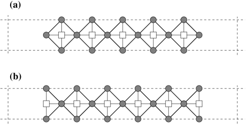
Figure 10: Supercell models of the SrO- (a) and TiO₂-terminated (b) SrTiO₃ slabs. Ti and O atoms are represented as white squares and gray circles respectively; Sr atoms are not shown. (Adapted from Ref. 27.)

In this Section we shall demonstrate the theory developed so far by applying it to SrTiO₃, one of the most important materials in the context of flexoelectricity, and the best known experimentally. In order to quantify the importance of surface effects, we shall consider a slab geometry, and two different lattice terminations (either of the SrO or TiO₂ type), as illustrated in Fig. 10.

1 General methodology

Our goal is to calculate the total flexovoltage response of either SrTiO₃ slab to a bending deformation in the limit of large thickness. We shall do this by taking into account the effect of full atomic relaxation, under the initial hypothesis that our slab behaves as a plate.  (We shall see in Sec. 3 that the beam-bending limit can easily be recovered by rescaling the plate-bending coefficient by a constant.) This requires the combination of three different computational frameworks, as detailed in the following.

Bulk calculations

Here we perform a number of calculations on a primitive unit cell of bulk SrTiO₃. This is primarily aimed at calculating the bulk flexoelectric tensor via a long-wave expansion of acoustic phonons. Acoustic phonons are treated at the linear-response level by means of density-functional perturbation theory as implemented in a modified version of the ABINIT package [29] in which the contribution of the macroscopic electric fields has been removed according to the discussion of Sec. 3. In particular, We choose a small star of wavevectors ${\bf q}$ surrounding the $\Gamma$ point in the Brillouin zone,

$${\bf q}=\frac{2\pi\tilde{q}}{a_{0}}(\pm 1,0;\,\pm 1,0;\,0),$$

and perform a full linear-response calculation for each of these points. (In practice, we make full use of symmetries to minimize the number of actual calculations.) Next, we perform a long-wave expansion of the charge-density response and interatomic force constants and extract the second-order-in-$\bf q$ coefficients via numerical differentiation with respect to ${\bf q}$. We obtain: (i) the flexoelectric force-response tensor $T^{\kappa}_{\alpha\lambda,\beta\gamma}$ via Eq. (31), from which $C^{\kappa}_{\alpha\lambda,\beta\gamma}$ and then the internal-strain tensor $L^{\kappa}_{\alpha\lambda,\beta\gamma}$ are constructed via Eqs. (34-35); and (ii) the charge-density response tensors $Q^{(1,\gamma)}_{\kappa\beta}$ and $Q^{(3,\gamma\lambda\sigma)}_{\kappa\beta}$, corresponding respectively to the Born effective charge tensor $Z^{*}_{\kappa,\beta\gamma}$ and the dynamical octupole tensor, via Eq. (45).

By combining the internal-strain tensor with the Born effective charges one can readily obtain the lattice-mediated contributions to the flexoelectric tensor as explained in Sec. 2. The octupole tensor, on the other hand, provides us with only partial information on the electronic (frozen-ion) flexoelectric tensor. In particular, only the longitudinal component of the electronic flexoelectric tensor, $\bar{\mu}_{\hat{\bf q}}$, along an arbitrary direction $\hat{\bf q}$ can be inferred from the two linearly independent entries of $Q^{(3,\gamma\lambda\sigma)}_{\kappa\beta}$. Following Hong and Vanderbilt [14], we define

$$\bar{\mu}_{\rm L1}=\bar{\mu}_{(100)},\qquad\bar{\mu}_{\rm L2}=2\bar{\mu}_{(110)}-\bar{\mu}_{(100)}.$$

These are related to the components of the type-II flexoelectric tensor, $\mu_{\rm L2}$ by [27]

$$\bar{\mu}^{\rm II}_{xx,xx} = \bar{\mu}_{\rm L1},$$ (142)

$$\bar{\mu}^{\rm II}_{xx,yy}+2\bar{\mu}^{\rm II}_{xy,xy} = \bar{\mu}_{\rm L2}.$$ (143)

Thus, in order to determine the transverse and shear components $\bar{\mu}^{\rm II}_{xx,yy}$ and $\bar{\mu}^{\rm II}_{xy,xy}$ independently, an additional calculation is necessary; this will be addressed shortly in Sec. 1.

In addition to the above calculations, which are based on the methodology described in this Chapter, we also need a bulk-level calculation of some auxiliary quantities by means of more established techniques. Specifically, we extract the high-frequency dielectric constant $\bar{\epsilon}_{\rm r}$ from a separate linear-response treatment of the electric-field perturbation. At the same time we obtain a redundant set of $Z^{*}_{\kappa,\beta\gamma}$ tensor elements, which are useful for assessing the quality of the numerical differentiation at first order in $\bf q$ performed in Sec. 1 above. Similarly, we carry out an independent calculation of the elastic tensor $C_{\alpha\lambda,\beta\gamma}$ via finite differences with respect to applied strain; this allows us to check the second-order-in-$\bf q$ calculations of the force-response tensors $C^{\kappa}_{\alpha\lambda,\beta\gamma}$, since these quantities are directly related by the sum rule in Eq. (36).

Truncated-bulk slab calculations

Here we carry out calculations similar to those of Sec. 1, but now on a slab supercell. This step is aimed at determining the transverse and shear components of the bulk electronic (frozen-ion) flexoelectric tensor.  In fact, the two independent components of the bulk dynamical octupole tensor $Q^{(3,\gamma\lambda\sigma)}_{\kappa\beta}$ that we calculated above are not sufficient to determine the three independent entries of the bulk $\bar{\mu}^{\rm II}_{\alpha\lambda,\beta\gamma}$ tensor. We are able to circumvent this limitation by recourse to a series of calculations on a slab geometry in which we determine the charge-density response, both in the bulk and at the surface, to longitudinal, transverse and shear strain gradients. A calculation of the flexoelectrically induced open-circuit electric field in the interior of the film, which relates [based on Eq. (50)] directly to the corresponding component of the bulk flexoelectric tensor in two cases out of three (longitudinal and transverse), allows us to obtain the missing component  of $\bar{\bm{\mu}}^{\rm II}$. The key point here is that the missing divergence-free component of the induced polarization current, which is not currently available from bulk-level calculations, manifests itself as a surface charge density, whose influence is readily apparent in the slab supercell geometry. Note that the specifics of the surface structure should not matter in these calculations. Thus, we choose the geometry that ensures the best convergence of the inner open-circuit field as a function of slab thickness, i.e., a truncated-bulk structure. (We perform such an analysis on both SrO- and TiO₂-terminated slabs, in order to verify that the results are indeed surface-independent as we expect.)

In practice, we use the same star of ${\bf q}$-points surrounding $\Gamma$ as in the bulk calculations described above. This time, however, we neglect the information on the force constants and only focus on the charge-density response of the system. We need to analyze such a response at the microscopic level, by using the curvilinear-coordinate formalism of Sec. 7 and Sec. 8. Of the two relevant response functions, $\rho^{\rm U}(x)$ and $\rho^{\rm G}(x)$, only the latter is really an issue, as $\rho^{\rm U}(x)$ can be straightforwardly calculated as the response to a uniform strain.  The result of the second-order Taylor expansion in ${\bf q}$ yields $\rho^{\rm G}(x)$, and this (together with $\rho^{\rm U}$) is then used to calculate the electric-field response functions $E^{\rm U,G}(x)$.

Note, however, that due to the removal of the macroscopic electric fields in the phonon calculations [13, 15, 27] (as required to perform the aforementioned Taylor expansions in ${\bf q}$, see Sec. 3), short-circuit electrical boundary conditions are enforced by construction on the calculated $\rho^{\rm G}$ and $E^{\rm G}$. This means that there are nonvanishing macroscopic electric fields in both the vacuum and the slab interior, and these fields show an undesirable dependence on the supercell geometry (vacuum and slab thicknesses). To have a physically well-defined (and geometry-independent) value of the internal field we need to enforce open-circuit electrical boundary conditions. We do this by applying an external field to the system that is exactly opposite to the calculated vacuum field. To determine the charge redistribution induced in the system upon application of an external field, we perform a separate linear-response calculation of the local electric field response to a macroscopic electric displacement field $D$. This is nothing but the local inverse dielectric permittivity of the slab supercell,

$$\frac{\partial E_{x}(x)}{\partial D_{x}}=\frac{1}{\epsilon_{0}}\bar{\epsilon}_{\rm r}^{\,-1}(x).$$

We then use

$$E^{\rm G,OC}_{x}(x)=E^{\rm G,SC}_{x}(x)-E^{\rm G,SC}_{x}(+\infty)\bar{\epsilon}_{\rm r}^{\,-1}(x),$$

where $x=+\infty$ corresponds, as usual, to the vacuum region. When referring to $E^{\rm G}(x)$ in the following, we shall implicitly assume that we are speaking of the open-circuit version $E^{\rm G,OC}_{x}(x)$.

Relaxed-ion slab calculations

Now that we have all the necessary bulk-specific information in hand, we still need to determine the surface-specific contributions to the flexovoltage coefficient $\varphi^{\rm surf}_{xx,{\rm eff}}$.  We shall compute $\varphi^{\rm surf}$ as the induced electrostatic potential offset upon application of a uniform effective strain ($\varepsilon_{yy}=\varepsilon_{{\rm eff}};\,\,\varepsilon_{xx}=-\nu\varepsilon_{{\rm eff}}$) to a free-standing slab with (001) surface orientation. This quantity can be conveniently accessed by means of a standard plane-wave code; no linear-response features are needed. In particular, we take a slab supercell corresponding to a periodic lattice of alternating SrTiO₃ and vacuum layers, and first calculate the electronic and structural ground state by setting the in-plane lattice parameter to the equilibrium bulk value. We then apply a small positive or negative strain of the type

$$\bm{\varepsilon}=\frac{\varepsilon_{\rm eff}}{2}\left(\begin{array}[]{r @{\quad} r @{\quad} r}-2\nu&0&0\\ 0&1&0\\ 0&0&1\end{array}\right),$$

where $\varepsilon_{\rm eff}$ is a small dimensionless number, typically $\varepsilon_{\rm eff}(\pm)=\pm 0.001$. (We find it computationally advantageous to preserve the fourfold axis of the SrTiO₃ surface by applying an isotropic in-plane strain.)

In each perturbed configuration, we first calculate the electronic ground state with the reduced coordinates of the atoms kept fixed to their unperturbed values; the resulting electrostatic potential profile is then processed by means of macroscopic averaging [17, 26] to extract the perturbed frozen-ion (FI) surface potential offsets. Next, we let the atoms relax to their new equilibrium positions in the strained lattices, and repeat the macroscopic averaging procedure to obtain the relaxed-ion (RI) offsets. Finally, we numerically differentiate the perturbed offsets (both FI and RI) to obtain their corresponding first-order variation,

$$\varphi^{\rm surf}=\frac{\phi(+)-\phi(-)}{2|\varepsilon_{\rm eff}|},$$

where $\phi(\pm)$ refers to the surface potential offset at positive or negative strain.  This procedure readily yields the RI and FI values of $\varphi^{\rm surf}$. The lattice-mediated (LM) values are simply calculated as the difference of the RI and FI ones. Of course, the slab needs to be sufficiently thick in order for the inner layers to be truly bulk-like, i.e., unaffected by the atomic distortions that originate from the surface truncation of the bonding network.

2 Computational parameters

We use the local-density approximation [30] to density-functional theory. The interactions between valence electrons and ionic cores are described by separable norm-conserving pseudopotentials in the Troullier-Martins [31] form, generated with the fhi98PP code. [32] The $4s^{2}4p^{6}$ and $3s^{2}3p^{6}$ shells of Sr and Ti, respectively, are explicitly treated as valence electrons. The reference states (numbers in parentheses indicate the core radius in bohr) of the isolated neutral atom used in the pseudopotential generation are $2s$(1.4), $2p$(1.4) and $3d$(1.4) for O, $4s$(1.5), $4p$(1.5) and $4d$(2.0) for Sr and $3s$(1.3), $3p$(1.3) and $3d$(1.3) for Ti. The local angular-momentum channel is $l=2$ for Sr and O and $l=0$ for Ti. The rigid-core corrections of Eq. (60) are not included in the presented results. The cutoff for the wavefunction plane-wave basis is set to 150 Ry in the slab calculations. (A test calculation with a 300 Ry cutoff did not show appreciable changes in the calculated electronic response functions; the 300 Ry cutoff was, nonetheless, necessary to ensure satisfactory accuracy in the force-response tensor at the bulk level.) The surface Brillouin zone of the slab supercell is sampled by means of a $8\times 8$ Monkhorst-Pack grid [33]; for the bulk primitive cell we use a sampling of up to $12\times 12\times 12$ $k$-points. The finite-difference parameter in the long-wave expansion, $\tilde{q}$, is set to 0.01 (tests with $\tilde{q}\!=\!0.02$ or $\tilde{q}\!=\!0.03$ indicated a convergence better than 1% in the calculated electronic response functions; smaller values of $\tilde{q}$ were found to yield less accurate results because of the excessive numerical noise). The lattice parameter of the cubic cell is set to $a_{0}$=7.268 bohr, which corresponds to the calculated equilibrium value.

The supercell models are based on the schematic illustrations of Fig. 10(a-b). For the truncated-bulk linear-response calculations we use 5.5-unit-cell (uc) thick SrTiO₃ slabs alternating with vacuum layers whose thickness is set to 2.5 uc. Of course, both (slab and vacuum) thicknesses are intended as convergence parameters in our calculations, whose scope is to describe the thermodynamic limit of a macroscopic slab. Tests with thinner slabs and thicker vacuum layers (up to 3.5 uc) showed optimal convergence for the aforementioned values of these parameters (again, better than 1%). For the relaxed-ion slabs, we use 7.5 uc-thick slabs with 3.5 uc-thick vacuum layers.

3 Results

Bulk calculations

Force-response tensor $C^{\kappa}_{\alpha\lambda,\beta\gamma}$ of bulk SrTiO₃ in short-circuit boundary conditions. O1, O2 and O3 refer to oxygen atoms forming $x$-, $y$- or $z$-oriented Ti-O-Ti bonds, respectively. All values are in eV. Atom $(xx,xx)$ $(xy,xy)$ $(xx,yy)$ Sr $-$24. 9 7. 9 $-$28. 7 Ti $-$67. 9 3. 8 $-$102. 3 O1 159. 3 15. 3 97. 4 O2 35. 2 17. 3 42. 3 O3 35. 2 $-$0. 9 30. 9

Summary of the linear-response data obtained from the long-wave (LW) approach at the bulk level, compared to the results of Hong and Vanderbilt [14] (HV) for the same quantities. Open-circuit electrical boundary conditions are enforced on the longitudinal response functions (L1 and L2). The force response to a shear strain gradient (S) is quoted in short circuit. The oxygen modes $\xi_{3}=x_{\rm O1}$ and $\xi_{4}=(x_{\rm O2}+x_{\rm O3})/\sqrt{2}$ are defined following Ref. 14. $\bar{\varphi}^{\rm bulk}$ is in V; other values are reported in eV. L1(LW) L1(HV) L2(LW) L2(HV) S(LW) S(HV) $\bar{\varphi}^{\rm bulk}$ $-$16. 15 $-$16. 25 $-$18. 07 $-$18. 17 - - Sr 16. 3 17. 0 33. 2 35. 7 7. 9 8. 4 Ti 49. 1 52. 3 36. 3 38. 9 3. 8 3. 0 $\xi_{3}$ 67. 2 68. 7 24. 9 13. 1 15. 3 15. 7 $\xi_{4}$ 3. 0 3. 6 22. 7 18. 2 11. 6 12. 0

Calculated Born effective charges and dielectric properties of bulk SrTiO₃. $Z^{*}_{\rm Sr}$ $Z^{*}_{\rm Ti}$ $Z^{*}_{\rm O1}$ $Z^{*}_{\rm O2}$ $Z^{*}_{\rm O3}$ $\bar{\epsilon}_{\rm r}$ $\epsilon_{\rm r}$ (static) 2. 5548 7. 2455 $-$5. 7027 $-$2. 0488 $-$2. 0488 6. 1785 1657

In Table 3 we report the relevant values of the force-response tensor of bulk SrTiO₃, calculated by using the long-wave method described in Sec. 2. In Table 3 we compare the above physical quantities to the analogous ones that were calculated in Ref. 14. To perform the comparison we first recast the force-response components into a tensorial representation that follows the same prescriptions as Eq. (142) and (143),

$$C^{\kappa}_{\rm L1} = C^{\kappa}_{xx,xx},$$ (144)

$$C^{\kappa}_{\rm L2} = C^{\kappa}_{xx,yy}+2C^{\kappa}_{xy,xy}.$$ (145)

Then, we convert the longitudinal quantities L1 and L2 from fixed-$\bf E$ or short-circuit (SC) to fixed-$\bf D$ or open-circuit (OC) boundary conditions by using [see Eq. (106) of Ref. 14]

$$C^{\kappa}_{\rm L}({\rm OC})=C^{\kappa}_{\rm L}({\rm SC})-\bar{\varphi}^{\rm bulk}_{\rm L}Z^{*}_{\kappa},$$ (146)

where $Z^{*}_{\kappa}$ is the Born effective charge (calculated values are reported in Table 3), $\bar{\varphi}^{\rm bulk}_{\rm L}$ is the purely electronic flexovoltage coefficient, and L stands for either L1 or L2. The calculated values of $\bar{\varphi}^{\rm bulk}_{\rm L1,L2}$ are also reported in Table 3 for direct comparison to those reported by Hong and Vanderbilt [14]. The agreement is overall very good, especially considering the different computational strategy, first-principles code and pseudopotentials that were used in Ref. 14.

Calculated elastic tensor of bulk SrTiO₃. The two rows refer to the bulk force-response calculation (“Force”) and to a direct bulk calculation where we took finite differences of the calculated stress tensor while varying the strain around the equilibrium cubic configuration (“Strain”). Values are in GPa. Method $(xx,xx)$ $(xy,xy)$ $(xx,yy)$ Force 385. 3 122. 2 111. 7 Strain 386. 2 122. 4 112. 6

As a numerical test of the calculated force-response tensor (Table 3), in Table 3 we report the elastic constants of bulk SrTiO₃ that we computed in two different ways: either as a first derivative of the stress with respect to the applied strain (“strain”) or by using the sum rule of Eq. (36) (“force”). The agreement is excellent (better than 1%), confirming the high numerical quality of the calculation. Note that the choice of the electrical boundary conditions is irrelevant for this test, as the sublattice sum of the atomic forces induced by a hypothetical electric field vanishes due to the acoustic sum rule.

Truncated-bulk slab calculations

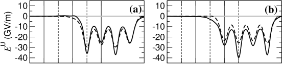
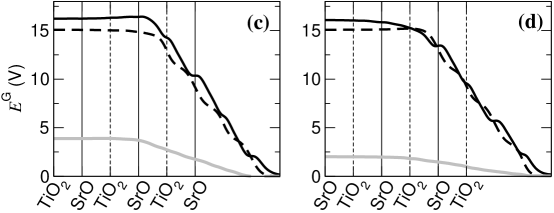
Figure 11: Electric field response to mechanical deformations. The $E^{\rm U}_{x}$ (a-b) and $E^{\rm G}_{x}$ (c-d) response functions are shown for a SrO- (a,c) and TiO₂-terminated (b,d) slab. Solid black, dashed black and solid gray curves refer to longitudinal, transverse and shear deformations, respectively. The location of the SrO (dashed) and TiO₂ (solid) atomic layers is indicated by vertical lines (only half of the symmetric slab is shown). (Adapted from Ref. 27.)

Frozen-ion flexovoltage coefficients of a truncated-bulk SrTiO₃ slab. To compute $\varphi^{\rm bulk}$ we used $\varphi^{\rm bulk}_{\rm L1,L2}$ as reported in Table 3 and $E^{\rm slab}_{xx,yy}=15.08$ V [extracted from Fig. 11(c-d)]. (L), (T) and (S) stands for longitudinal, transverse and shear, respectively. Units of Volts are used throughout. $\varphi^{\rm bulk}$ $\varphi^{\rm surf}$ $\varphi$ (total) SrO TiO₂ SrO TiO₂ $xx,xx$ (L) $-$16.15 14.36 16.95 $-1$.80 0.80 $xx,yy$ (T) $-$15.08 15.68 12.45 0.61 $-2$.63 $xy,xy$ (S) $-$1.50 $-2$.38 $-$0.51 $-3$.88 $-2$.01

Table 1:

In Fig. 11(a-d) we plot the calculated $E_{x}^{\rm U,G}(x)$, corresponding to either a SrO- or a TiO₂-terminated slab and to each of the three types of imposed strain gradients shown in Fig. 6 (with no internal relaxations allowed). As anticipated in Sec. 8, there is an important qualitative difference between the case of the longitudinal or transverse response, where the strain gradient is oriented along the surface normal, and that of the shear response, where it is directed in plane.

In the former case, $E_{x,\beta\beta}^{\rm U}(x)$ (describing the ${\bf E}$-field response to a uniform strain) yields the surface contribution to the flexovoltage coefficient, $\bar{\varphi}^{\rm surf}_{xx,\beta\beta}$, via Eq. (128),  while the functions $E_{xx,\beta\beta}^{\rm G}(x)$ provide us with the sought-after information on the bulk flexovoltage coefficient of SrTiO₃,

$$\varphi^{\rm bulk}_{xx,\beta\beta}=-E^{\rm G}_{xx,\beta\beta}(x=0).$$

Note that the $E_{xx,\beta\beta}^{\rm G}(x)$ functions are roughly uniform inside the film, which indicates that the slab is thick enough to display bulk properties therein, and zero outside, consistent with the open-circuit electrical boundary conditions that were enforced. Moreover, the uniform internal field appears to be nicely independent of the surface termination for the longitudinal and transverse deformations, which is a further important consistency test for our computational approach.

In the shear case, however, the flexoelectric field depends on both bulk and surface-specific properties, [15] and such a termination dependence is clear from a comparison of the gray curves in Fig. 11(c) and (d). From the electric-field response functions of Fig. 11(c-d) we can thus only extract the total flexovoltage coefficient of the slab, $\varphi_{xy,xy}=-E^{\rm G}_{xy,xy}(x=0)$. To separate $\varphi_{xy,xy}$ into bulk and surface terms it suffices, however, to complement the above data with the $\varphi^{\rm bulk}_{\rm L1,L2}$ values that we calculated at the bulk level. Indeed, by replacing the flexoelectric tensor components in Eq. (142) and Eq. (143) with the corresponding flexovoltage coefficients, we have

$$\varphi^{\rm bulk}_{\rm L1} = \varphi^{\rm bulk}_{xx,xx},$$ (147)

$$\varphi^{\rm bulk}_{\rm L2} = \varphi^{\rm bulk}_{xx,yy}+2\varphi^{\rm bulk}_{xy,xy}.$$ (148)

Eq. (147) constitutes a useful consistency check of the methodology, as $\varphi^{\rm bulk}_{\rm L1}$ is redundant with the already calculated value of $\varphi^{\rm bulk}_{xx,xx}$. Eq. (148), on the other hand, yields the desired value of $\varphi^{\rm bulk}_{xy,xy}$ since we already know $\varphi^{\rm bulk}_{xx,yy}$ from the slab calculations. Finally, we use $\varphi_{xy,xy}=-E^{\rm slab}_{xy,xy}$ to infer $\varphi^{\rm surf}_{xy,xy}=\varphi_{xy,xy}-\varphi^{\rm bulk}_{xy,xy}$.

Our results for the bulk, surface, and total flexovoltage coefficients of the truncated-bulk, frozen-ion deformation of a SrTiO₃ slab are summarized in Table 1. At the bulk level, it is interesting to note the relatively small magnitude of the shear coefficients $\varphi^{\rm bulk}_{xy,xy}$ and $\varphi^{\rm surf}_{xy,xy}$ compared to both the longitudinal and the transverse ones. Meanwhile, in the latter two cases there is a substantial cancellation between bulk and surface terms; as a result, the values of the total flexovoltage coefficients $\varphi$ are all comparable in magnitude. This fact can be rationalized by observing that the linear response to atomic displacements in a ionic (or partially ionic) solid is largely dominated by the rigid displacement of an approximately spherical charge density distribution surrounding each atom. The spherical contribution, which is typically large and negative, [12] shows up in $\varphi^{\rm bulk}_{xx,\beta\beta}$, and with opposite sign in $\varphi^{\rm surf}_{xx,\beta\beta}$; in the shear case neither the bulk nor the surface term are affected (see Sec. 5). Remarkably, the resulting values of $\varphi$ depend strongly on the details of the surface, and in some cases even have opposite signs in the SrO- and TiO₂-terminated slabs. Such a conclusion, in fact, persists after we take into account the full relaxation of the atomic structure; we shall demonstrate this point in the following paragraphs.

Relaxed-ion slab calculations

Flexovoltage coefficients of a relaxed SrTiO₃ slab. The frozen-ion (FI), lattice-mediated (LM) and total relaxed-ion (RI=FI+LM) values of the bulk, surface and total slab response are reported. Units of Volts are used throughout. $\varphi^{\rm bulk}$ $\varphi^{\rm surf}$ $\varphi$ (total) SrO TiO₂ SrO TiO₂ FI $-$10.37 13.47 6.84 3.10 $-$3.53 LM $-$0.44 $-$4.93 5.34 $-$5.38 4.90 RI ${-10.81}$ 8.53 12.18 ${\bf-2.28}$ ${\bf 1.37}$

The results of the relaxed-ion slab calculations allow us to complete the picture of the fully relaxed flexovoltage response of a SrTiO₃ slab in the plate-bending limit. [The beam-bending case is easily recovered by multiplying the reported values by $\tau=\mathcal{C}_{xx,xx}/(\mathcal{C}_{xx,xx}+\mathcal{C}_{xx,yy})$. By using the calculated elastic constants of bulk SrTiO₃, reported in Table 3, we find $\tau=0.77$.] A summary of the results is reported in Table 3. The respective contributions of the bulk and surface are, overall, in line with the available order-of-magnitude estimates. [34] The values shown in bold font, i.e., the total flexovoltage coefficients of the two types of slab, comprise the main result of this work. Note that they depart substantially from the corresponding bulk coefficient, confirming the dramatic impact of the surface structural and electronic properties on the electromechanical response of the system. In fact, the aforementioned response coefficients are even opposite in sign depending on whether a SrO- and TiO₂-terminated slab is considered. This is a remarkable result, as it means that an atomically thin surface termination layer can modify, and even reverse, the flexovoltage response of a macroscopically thick sample. This constitutes a rather drastic departure from the characteristics of other electromechanical phenomena (e.g., piezoelectricity), where the details of the surfaces typically become irrelevant in the thermodynamic limit.

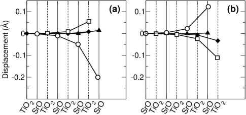
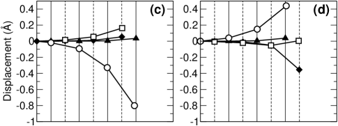
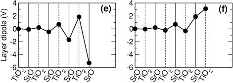
Figure 12: Static and induced ionic relaxations at the SrTiO₃ surface. (a-b): Ionic relaxations in the unperturbed slabs (displacements from ideal bulk-like sites). Circles, squares, diamonds and triangles correspond, respectively, to Sr, Ti, O(Ti) and O(Sr) atoms. (Cations are indicated by empty symbols, oxygen atoms by filled ones.) Negative values indicate inward displacements (i.e., towards the slab center). (c-d): Displacements induced by a uniform strain of the type $\varepsilon_{yy}-\nu\varepsilon_{xx}$; for the two oxygen atoms in the TiO₂ layers, only one value (their average displacement) is shown. (e-f) Layer-by-layer decomposition of the lattice-mediated contribution to the induced surface potential offset. Vertical lines indicate the position of the SrO (solid) and TiO₂ (dashed) atomic planes. (Adapted from Ref. 27.)

It is interesting to note that the surface shows an even larger termination dependence at the frozen-ion level, but with opposite sign. The LM contribution to $\varphi^{\rm surf}$ is indeed large, and depends so strongly on the termination that its inclusion results in a voltage reversal, both in the TiO₂- and SrO-type slabs. (By contrast, the LM contribution to the bulk flexovoltage coefficient is relatively minor, about one order of magnitude smaller than any other value reported in the table, and has little impact on the final results.) To illustrate the reason for such a strong dependence, a microscopic analysis of the surface relaxations is provided in Fig. 12. In the SrO case, the layer-by-layer decomposition of the induced dipole shown in Fig. 12(e) has an oscillatory behavior whose amplitude decays exponentially as a function of the distance from the surface; as a consequence, the surface layer clearly dominates the overall response.  Instead, for the TiO₂-terminated slab shown in Fig. 12(f), the surface layer responds with a positive dipole instead of a negative one, in sharp contrast to the “underdamped” oscillatory behavior in Fig. 12(e). This behavior is probably due to the alteration of the bonding network, which we speculate to be much more profound at the TiO₂-type surface than at the SrO-type one, whereby the boundary atoms no longer behave as bulk-like but rather as a distinct chemical entity.

Apart from the obvious relevance of the above observations to the physics of SrTiO₃ surfaces, the analysis of Fig. 12(e-f) carries a general message that we have already anticipated in the above paragraphs. Any single atomic layer near the surface has a remarkably large contribution to $\varphi^{\rm surf}$, sometimes of the same order as (or even larger than) the overall flexovoltage response of the slab. In fact, the total open-circuit voltage results from the subtle cancellation of many contributions of dissimilar physical nature. This implies that exceptional care is needed when dealing with flexoelectric phenomena, either when performing the calculations or when interpreting the experiments.

4 Conclusions and outlook

In this Chapter we have described the main advances in the first-principles theory of flexoelectricity that have taken place during the past five years. The progress that emerges from these pages is undoubtedly impressive – we are at the stage where the full flexoelectric response of real materials, including bulk and surface effects, can be calculated ab initio with great accuracy. Still, much remains to be done before the field can be regarded as mature. We discuss here several research avenues that we identify as being of pivotal importance for future progress.

• Theory of the current-density response. The most fundamental and complete framework for the theory of flexoelectricity is the current-response formalism introduced in Sec. 2. Unlike the charge-response formalism summarized in Sec 5, the current-response approach is capable in principle of resolving all independent components of the flexoelectric tensor. However, two issues remain to be settled in relation to this approach. First, direct methods for obtaining the current response functions $\overline{P}_{\kappa\beta}^{\bf q}$ of Eq. (13) by computing the linear response to a phonon of small but finite wavevector $\bf q$ have not yet been developed and tested. Once implemented, this would allow for a finite-difference calculation of the $\overline{P}_{\alpha,\kappa\beta}^{(2,\gamma\lambda)}$ of Eq. (14), and thence, the electronic contribution in Eq. (18). Second, some aspects of the connection between the current-response theory and the theory of charge responses (including surface charges) remain to be clarified, as discussed in the context of Eq. (50) and following Eq. (101). A solution of these two issues would help put the theory of flexoelectricty on a truly sound footing.

• Analytic derivation of the ${\bf q}$-expansions. The conceptual foundation of most of the material treated in this Chapter is a long-wave expansion of certain physical observables as a function of the wavevector ${\bf q}$ of an acoustic phonon. The calculations described in Sec. 3 were performed by taking such a ${\bf q}$-expansion numerically via finite differences, which is computationally cumbersome. Ideally, it would be best to perform the expansion analytically, i.e., to derive the DFPT equations that directly yield the wavefunction response to a strain gradient perturbation. This would also be desirable in the context of the direct current-density implementation sketched just above. When implemented in an existing DFPT code, such methods would allow for a more straightforward calculation of flexoelectric properties of materials, and thus foster a more widespread application of these techniques within the research community.

• Application to complex materials. Our focus in this chapter has been on materials with cubic symmetry. Clearly a proper theory that also covers crystals of lower symmetry is strongly required. The extension of the theory to such materials will require attention not just to the proliferation of independent parameters in the flexoelectric tensor, but also to subtle physical issues having to do, for example, with the anisotropic electronic screening that occurs when the symmetry is reduced. In the case of crystals that are piezoelectric (and possibly also polar), care will be needed to separate the higher-order flexoelectric from dominant piezoelectric (and possibly spontaneous) polarization response. The application to insulating ferromagnets or antiferromagnets should introduce no special difficulties in most cases, but may involve subtleties for magnetoelectric crystals or when spin-orbit coupling is strong. A first-principles theory of flexomagnetism has yet to be developed.

• Compositional gradients. An electric polarization can also arise in the presence of a compositional gradient, e.g., in Ba_1-xTi_xO₃ films.[35] To our knowledge, a proper theory of such an effect is lacking. Since a compositional gradient generally also entails a strain gradient, some care will be called for in separating these effects and computing them independently before combining the contributions to make physically meaningful predictions.

• Connection to higher-level models. With the techniques described here, one can in principle calculate the fundamental flexoelectric properties of an arbitrary material. To use this information in real physical problems, however, one typically has to deal with many additional issues that are intractable by means of direct first-principles simulation: large samples with complex shapes, temperature effects, etc. It would be very desirable in this context to be able to extract the relevant physical parameters from the ab initio calculations, and incorporate them in some higher-level theory (e.g. atomistic, effective Hamiltonian, or continuum) where length- and time-scale limitations are much less stringent. A successful attempt in this sense has already been reported; [36] still, consistently incorporating the latest first-principles developments into macroscopic theories remains an open challenge. For example, it would be of crucial importance, for a realistic description of the flexoelectric effect, to extract the relevant surface-specific properties from the density-functional calculations, and incorporate them into the higher-level model. Making progress in this direction will also promote a closer interaction between different communities working on flexoelectricity (continuum numerical modeling, Landau theory, etc.), which we believe would have a strong positive impact on the field.

In summary, there has been dramatic progress in the development of a full first-principles theory of flexoelectricity. Several important challenges remain, as discussed above, but at least these have been identified, and solutions appear to be within reach. In any case, the development of the theory of flexoelectricity has already revealed many fascinating links to other, at first sight unrelated, research areas (e.g., the relationship to transformation optics, where the use of curvilinear coordinates facilitates the solution of complex electrical engineering problems). We believe that more surprises are in store, and will progressively emerge while further progress is made along the above lines. As the study of flexoelectricity touches so many subfields of condensed matter physics, we expect cross-cutting progress that will likely benefit the first-principles materials theory community at large. All in all, we look forward to the day when predictive calculations of flexoelectric responses can become a routine part of the tool-kit of first-principles computational materials theory.