Compactification tuning for nonlinear localized modes in sawtooth lattices

Abstract

We discuss the properties of nonlinear localized modes in sawtooth lattices, in the framework of a discrete nonlinear Schrödinger model with general on-site nonlinearity. Analytic conditions for existence of exact compact three-site solutions are obtained, and explicitly illustrated for the cases of power-law (cubic) and saturable nonlinearities. These nonlinear compact modes appear as continuations of linear compact modes belonging to a flat dispersion band. While for the linear system a compact mode exists only for one specific ratio of the two different coupling constants, nonlinearity may lead to compactification of otherwise non-compact localized modes for a range of coupling ratios, at some specific power. For saturable lattices, the compactification power can be tuned by also varying the nonlinear parameter. Introducing different on-site energies and anisotropic couplings yield further possibilities for compactness tuning. The properties of strongly localized modes are investigated numerically for cubic and saturable nonlinearities, and in particular their stability over large parameter regimes is shown. Since the linear flat band is isolated, its compact modes may be continued into compact nonlinear modes both for focusing and defocusing nonlinearities. Results are discussed in relation to recent realizations of sawtooth photonic lattices.

I Introduction

The creation and manipulation of nonlinear localized lattice excitations (“discrete solitons” or “discrete breathers”) is of interest in many areas of physics FG08 , and in particular within nonlinear optics Lederer08 . In many contexts, one strives for achieving optimal spatial localization. In the presence of linear dispersion (diffraction), resulting, e.g., from a linear (harmonic) coupling between neighboring sites, the localization will generically be exponential. However, non-generic situations may appear in presence of nonlinear dispersion, e.g., when the inter-site interaction also has a nonlinear contribution. In such situations, a proper control of the nonlinear effects may lead to a complete cancellation of the linear coupling between sites, resulting in exact “discrete compactons” fully localized at a small number of sites, with strictly zero tail (for examples, see, e.g., KK02 ; OJE03 ; AKS10 ). The experimental realization of these specific nonlinear interactions poses however serious challenges, and so far no direct observation of compactification of nonlinear lattice modes has, to the best of our knowledge, been reported.

On the other hand, it is well known that in certain lattices geometries, frustration effects make possible the existence of strictly compact modes even in absence of any nonlinearity. Such modes can be seen to result from destructive interference of couplings between different sites, and are typically associated with a flat linear dispersion band. A number of different examples of this scenario are discussed, e.g., in Refs. Derzhko10 ; HA10 ; Flach14 ; Liu14 , and references therein. In particular, recent experiments have being performed in two-dimensional (2D) Lieb photonic lattices, where different transport regimes lieb1 as well as the excitation of the localized flat band mode lieb2 ; lieb3 were observed. Maybe the most well known example is the 2D Kagome lattice, which supports modes strictly localized on six sites along a hexagonal geometry (see, e.g., BWB08 ). As was shown in Ref. VJ13 , these compact modes exist also in presence of a pure on-site nonlinearity, and indeed constitute an effective ground state of the system in the small-power regime for a defocusing Kerr (cubic) nonlinearity. However, above a rather small threshold power the compact modes destabilize, and transform into stable standard localized modes with exponential tails.

The compactification of linear modes due to competing linear interactions may appear also in one-dimensional (1D) settings, and a number of examples have been illustrated, e.g., in Refs. Derzhko10 ; Flach14 . One of the most studied 1D lattices is the sawtooth chain; see, e.g., SSWC96 ; SHSRC02 ; ZT04 ; HA10 ; Derzhko10 (also called $\Delta$ chain NK96 or triangle lattice HAM13 ; Flach14 ). Due to its construction from corner-sharing triangles, it is often considered as a 1D analogue of the Kagome lattice, and is one of the simplest possible lattices allowing for compact linear modes and a flat band, which makes it particularly attracting for experimental realizations. A compact mode in a similar setting was used to experimentally observe a Fano resonance Weimann13 . Very recently, the linear properties of a sawtooth photonic lattice, created using the femtosecond laser written technique, were also studied experimentally photonics14 . Furthermore, the dependency of coupling constants of these lattices on polarization Rojas14 provides ample and tunable opportunities beyond geometric considerations. This is important since, in contrast to the Kagome lattice, compactification in a linear sawtooth lattice appears only at one specific (irrational) ratio between the two different coupling constants (horizontal and diagonal), which again poses an experimental challenge for fine-tuning. However, as we will show in this work, nonlinearity allows the existence of compact modes for different coupling ratios, which certainly would facilitate the observation of highly localized states in a real experiment.

The aim of the present paper is to illustrate how nonlinearities and other effects can be used for the purpose of facilitating the compactification tuning of localized modes in sawtooth lattices. In Sec. II we describe the general model, using the discrete nonlinear Schrödinger (DNLS) equation with a general on-site nonlinearity and linear coupling constants representing the sawtooth geometry. We discuss the linear dispersion relation and its flat-band structure, and obtain the general conditions on the geometry for existence of 3-site compactons as exact stationary solutions. In Sec. III we specialize to power-law nonlinearities, and obtain an expression for the power needed for compactification, valid for a whole range of ratios for the linear coupling constants. For the physically most interesting case of cubic Kerr-nonlinearity (focusing or defocusing), we perform a detailed numerical analysis of localized modes (not restricted to compactons) in Sec. III.1, illustrating explicitly how certain, linearly stable, localized modes compactify when the appropriate relation between coupling ratios and power is fulfilled. Another physically important case of a saturable nonlinearity is analyzed in Sec. IV. The saturability introduces another parameter which can be employed, together with the power, for compactification tuning, and we illustrate the scenarios in different regimes analytically as well as numerically, particularly showing the existence of strongly localized, stable modes over large parameter regimes. Finally, Sec. V discusses two additional generalizations of the sawtooth lattice with cubic nonlinearity, yielding further possibilities for compactification tuning: on-site energy alternations (Sec. V.1) and coupling anisotropies (Sec. V.2). Conclusions are given in Sec. VI.

II Model and general compacton conditions

We consider the following form of the discrete nonlinear Schrödinger equation on a sawtooth lattice sketched in Fig. 1,

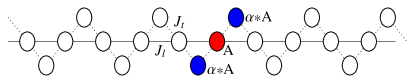
Figure 1: (Color online) Geometry of the sawtooth lattice with its compact mode (white circles imply zero amplitudes).

$$i\dot{u}_{n}+\sum_{m\neq n}J_{n,m}u_{m}+\gamma f(|u_{n}|^{2})u_{n}=0\ ,$$ (1)

where $n=1,2,\dots,N$. The coupling $J_{n,m}$ denotes the interactions between the site $n$ and its connected lattice sites $m$, with diagonal (“tip”) couplings $J_{t}$ and horizontal (“line”) couplings $J_{l}$. The function $f(x)$, describing a general on-site nonlinearity with strength $\gamma$, is at this point arbitrary. We may put $f(0)=0$, since any homogeneous linear on-site potential may be removed by a gauge transformation (extensions to non-homogeneous on-site potentials will be discussed in Sec. V). Generally, the parameters $J_{l}$, $J_{t}$ and $\gamma$ may be complex-valued (describing effects of gain and/or loss), but in our explicit examples in Secs. III-V we will only consider real-valued cases. We should remark that the geometry in Fig. 1 apparently differs from that usually associated with sawtooth lattices NK96 ; SSWC96 . Instead of taking equally oriented triangles, we take the triangle tips to point alternately up and down from the horizontally line-coupled sites. In this way, we avoid the otherwise physically unavoidable interaction between neighboring vertices, describing a more appropriate experimental realization of a photonic sawtooth lattice photonics14 . This obviously does not change the mathematical model, which in both cases only contains the two nearest-neighbour couplings $J_{t}$ and $J_{l}$.

Looking for stationary solutions of the form

$$u_{n}(t)=a_{n}e^{i\lambda t}\ ,$$ (2)

the first term in Eq. (1) is replaced with $-\lambda u_{n}$. Assuming the line sites to be of odd $n$, whereas for the tips $n$ is even, then leads to the following set of equations in the linear regime ($\gamma|a_{n}|^{2}=0$):

$$\lambda a_{n}=J_{t}(a_{n+1}+a_{n-1})+\begin{cases}J_{l}(a_{n+2}+a_{n-2})&\text{ for $n$ odd\ ,}\\ 0&\text{ for $n$ even\ .}\end{cases}$$

The linear dispersion relation Derzhko10 ; HA10 ; photonics14 is computed by assuming a propagating plane wave $a_{n}=A{\rm e}^{ikn}$, obtaining for the linear frequencies, rescaled with the horizontal coupling constant $J_{l}$,

$$\bar{\lambda}_{\pm}(k;J) \equiv \lambda_{\pm}/J_{l}=$$

$$\cos(2k)\pm\sqrt{\cos^{2}(2k)+2J^{2}\left[1+\cos(2k)\right]}\ .$$

Here we have also introduced the rescaled, dimensionless coupling ratio $J\equiv J_{t}/J_{l}$, which is the essential system parameter that determines its qualitative physical properties in the linear regime.

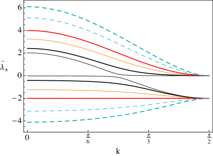
Figure 2: (Color online) Dispersion relation (II) for the sawtooth lattice for different coupling ratios: $J$= 0.1 (0.5, 1, $\sqrt{2}$, 2, 2.5) in thin black (thick black, thin orange, thick red, thin dashed, thick dashed).

As illustrated in Fig. 2, the lower band becomes flat at the particular coupling ratio $J=\sqrt{2}$ for which $\bar{\lambda}_{-}=-2$. It is important to note that the flat band existing at these parameter values is isolated from the upper band ($\bar{\lambda}_{+}=4\cos^{2}k$) with a bandgap of $2$. Thus, in contrast to the Kagome lattice studied in Ref. VJ13 , where the flat band is always attached to the edge of a dispersive band, we may here expect a resonance-free continuation of compact modes belonging to the flat linear band for focusing as well as for defocusing nonlinearities.

To obtain a condition for existence of compact stationary solutions (2) of Eq. (1) for general nonlinearities $f(x)$, we write an ansatz for the solution as a 3-site compacton (analogously to the linear flat-band modes Derzhko10 ; HA10 ; photonics14 ), with $a_{n_{0}}=A$ for the central, 4-bonded, “line site” (red disk in Fig. 1), and $a_{n_{0}\pm 1}=\alpha A$ for the two neighboring, 2-bonded, “tip sites” (blue in Fig. 1). The condition to have zero amplitude on the neighboring line sites $n_{0}\pm 2$, and thus also for the rest of the lattice, then gives immediately an expression for the amplitude ratio $\alpha$ in terms of the ratio between the coupling constants:

$$\alpha=-1/J\ .$$ (4)

For the central line site $n_{0}$, Eqs. (1)-(2) give the following expression for the rescaled frequency $\lambda/J_{l}$:

$$\lambda/J_{l}=-2+\frac{\gamma}{J_{l}}f(|A|^{2})\ .$$ (5)

The corresponding equations for the two tip sites $n_{0}\pm 1$ yield

$$\lambda/J_{l}=-J^{2}+\frac{\gamma}{J_{l}}f(|A/J|^{2})\ .$$ (6)

Eliminating $\lambda$ from Eqs. (5)-(6) gives an implicit, general condition to determine the central-site intensity $|A|^{2}$ in terms of the coupling ratio $J$ and the ratio $\gamma/J_{l}$ between nonlinearity strength and horizontal coupling constant:

$$\frac{\gamma}{J_{l}}\left(f(|A|^{2})-f(|A/J|^{2})\right)=2-J^{2}\ .$$ (7)

Obviously, in the linear limit $\gamma|A|^{2}\rightarrow 0$ and the left-hand side of Eq. (7) vanishes. This implies that $J_{t}\rightarrow\pm\sqrt{2}J_{l}$, recovering the linear flat-band condition. Using Eq. (4), we may also determine the total power, $P\equiv\sum_{n}|u_{n}|^{2}$, of the compacton as

$$P=\left(1+2|1/J|^{2}\right)|A|^{2}\ .$$ (8)

Apart form the power, the other conserved quantity of DNLS-like systems is the Hamiltonian

$$H=\sum_{n\neq m}J_{n,m}u_{n}^{*}u_{m}+\gamma\sum_{n}F(|u_{n}|^{2})$$ (9)

for the canonical variables $(u_{n},-iu_{n}^{*})$. The function $F(|u_{n}|^{2})$ defines the nonlinearity of the system ($f(x)=F^{\prime}(x)$) and will be specified later on. (Note that we chose here a sign-convention in accordance with the sign-convention used in the definition of the frequency $\lambda$ in (2). As illustrated below, stable compactons may then appear as ground states for defocusing nonlinearities.)

In order to compare how compactons are related to eventual ordinary localized stationary modes, which have nonvanishing tails, we implement a Newton-Raphson iterative method to find numerical solutions at a given accuracy. We will look for fundamental solutions centered at tip or line sites or in between sites, using periodic boundary conditions to avoid surface effects. A typical lattice size used numerically is $N=40$, while also checking the consistency of the results by varying the chain length. We generally use $J_{l}=1$ in all numerical calculations.

For any nonlinear stationary mode $\{a_{n}\}$ fulfilling (1)-(2), we perform a standard linear stability analysis sta : we use the ansatz $u_{n}(t)=[a_{n}+\epsilon_{n}(t)]e^{i\lambda t}$, and linearize equations in $\epsilon_{n}(t)$, giving access to the spectrum $\{\omega_{\rm l}\}$ of perturbations ${\rm e}^{i\omega_{\rm l}t}$. We define a stability parameter $g\equiv{\rm Max|Im(\omega_{l})|}$, which will be nonzero for unstable modes, whereas $g=0$ for stable solutions. To compare the localization properties of different modes, we use the participation number defined as

$$R\equiv\frac{P^{2}}{\sum_{n}^{N}|u_{n}|^{4}}\rightarrow\begin{cases}1&\text{for a single excited site,}\\ N&\text{for extended homogeneous profiles.}\end{cases}$$

This parameter gives a measure of the effective size of a given profile. In particular, for the compacton solution this formula reduces to

$$R_{c}=\frac{\left[\left|J\right|^{2}+2\right]^{2}}{\left|J\right|^{4}+2}\rightarrow\begin{cases}2&\text{ for }J\rightarrow 0\ ,\\ 1&\text{ for }J\rightarrow\infty\ .\end{cases}$$ (10)

From this, it also follows that the maximum compacton participation number $R_{c}=3$ would appear for $J\rightarrow 1$, when the profile would be equally distributed between all 3 sites. For the linear case, $R_{c}(|J|=\sqrt{2})=8/3$.

III Power-law nonlinearities

Specializing first to a general, pure power-law nonlinearity, we have $f(x)=x^{\sigma}$. Plugging this into Eq. (7) yields that an exact 3-site compacton exists when the following relation, between the central-site intensity and the coupling constants, is fulfilled:

$$\frac{\gamma|A|^{2\sigma}}{J_{l}}=\frac{2-J^{2}}{1-1/|J|^{2\sigma}}\ .$$ (11)

Using Eq. (8), we find that the compacton condition can alternatively be written in terms of the total power as:

$$P=\left(2+|J|^{2}\right)\left(\frac{J_{l}(2-J^{2})}{\gamma\left(|J|^{2\sigma}-1\right)}\right)^{1/\sigma}.$$ (12)

For power-law nonlinearities, $F(x)=x^{\sigma+1}/(\sigma+1)$ in Hamiltonian (9); for the compact mode we find

$$H_{c}\equiv\frac{H}{J_{l}}=$$ (13)

$$-\frac{4JP}{2+|J|^{2}}+\frac{\gamma/J_{l}}{\sigma+1}\left(1+\frac{2}{(-J)^{\sigma+1}}\right)\left(\frac{|J|^{2}P}{2+|J|^{2}}\right)^{(\sigma+1)/2}.$$

III.1 Localized modes for cubic nonlinearities

For the special case $\sigma=1$, which corresponds to a standard cubic (Kerr) nonlinearity, and real-valued coupling constants, Eq. (12) considerably simplifies. We can define an effective nonlinearity parameter as

$$\Gamma\equiv\frac{P\gamma}{J_{l}}=\frac{4-J^{4}}{J^{2}-1}\ .$$ (14)

For Kerr nonlinearities, $\Gamma$ is the only free parameter. Therefore, for focusing nonlinearities $\Gamma>0$, whereas $\Gamma<0$ for the defocusing case. We can also calculate the rescaled frequency of the (nonlinear) compacton, given by

$$\bar{\lambda}_{c}\equiv\frac{\lambda_{c}}{J_{l}}=\frac{J^{4}-2}{1-J^{2}}.$$ (15)

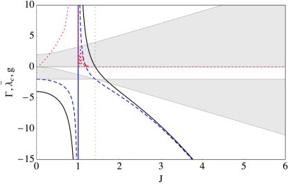
Figure 3: (Color online) Properties of the compacton: effective nonlinearity $\Gamma$ (solid), rescaled frequency $\bar{\lambda}_{c}$ (dashed) and stability parameter $g$ (dotted) vs. $J$. The linear band extension is shown with shaded areas. The analytical expressions for $\Gamma$ and $\bar{\lambda}_{c}$ are equivalent to those of a three-core coupler studied in SMTL92 for different regimes: $0<J<1\leftrightarrow\textrm{``branch c''}$; $1<J<\sqrt{2}\leftrightarrow\textrm{``branch b''}$; $J>\sqrt{2}\leftrightarrow\textrm{``branch d''}$.

The behavior of both $\Gamma$ and $\bar{\lambda}_{c}$ is shown in Fig. 3 with a solid black and dashed line, respectively. Furthermore, we show the stability parameter $g$ (red dotted) vs.  $J$. Whenever $g>0$, the solution is unstable. The linear band extensions are plotted as shaded background. When the linear compacton condition $J=\sqrt{2}$ is fulfilled, obviously $\Gamma(J)=0$ and $\bar{\lambda}_{c}=-2$. At this value, we observe that the lower band width becomes strictly zero, corresponding to the perfectly flat band of this lattice, occurring for this special geometric relation.

For $J>\sqrt{2}$, the linear band broadens but a compact mode still exists for negative $\Gamma$, with a frequency below the lower band. As is seen, the mode stays linearly stable, which was also confirmed by direct numerical integration of Eq. (1). In the large-$J$ limit, $|\alpha|$ decreases and the compacton, having its dominating amplitude on a line site, approaches a highly nonlinear single-site localized mode of an ordinary defocusing 1D chain (as the line-couplings become negligible next-nearest neighbor couplings), which is always stable.

On the other hand, for decreasing $J<\sqrt{2}$ compactons instead occur for a focusing nonlinearity ($\Gamma>0$) and with the frequency entering into the gap above the lower band. As can be seen, the mode initially remains linearly stable but becomes unstable in a bifurcation at $J\simeq 1.27$. The origin of this instability can be understood by comparing with the well-known properties of the stationary solutions of a three-core coupler with focusing nonlinearity (with open boundary conditions, i.e., without any surrounding lattice), studied, e.g., in Ref. SMTL92 . The analytical forms of the compactons in the sawtooth lattice are mathematically equivalent to those of the symmetric three-core eigenmodes given in SMTL92 ; however, the stability properties may differ due to additional possible resonances with the surrounding lattice. As the corresponding modes in the focusing three-core coupler (“branch b” with the notation of SMTL92 ) are always stable, the observed instabilities for the compacton in the focusing sawtooth lattice must originate in resonances between internal oscillations of the compacton core and linear oscillations of the surrounding chain. Decreasing $J$ further towards the singularity at $J=1$, stronger instabilities appear as the compacton frequency becomes positive and enters the upper linear band. Compactons with positive frequency, in a strongly nonlinear focusing lattice, are found to be always unstable.

From the above, we reach the important conclusion that there are stable compact nonlinear modes in direct continuation of the linear flat-band modes for both focusing and defocusing nonlinearities. At the singularity $J=1$ both $\Gamma$ and $\bar{\lambda}_{c}$ change sign, and we see that for $J<1$, compact modes with negative effective nonlinearity and frequency are always unstable. Noting that the anti-phased compact modes in this defocusing regime are mathematically equivalent to three-core in-phase modes with focusing nonlinearity, these instabilities are equivalent to those described in Ref. SMTL92 for the solution “branch c” (corresponding to main amplitudes at the two tip sites). Thus, this instability originates from an internal resonance between oscillation modes of the three-site compacton core. So to conclude this part, we see that for any sawtooth lattice geometry we can find a compact mode centered on a line site. This mode is stable for a wide window in parameter space but destabilizes when the surrounding tip site amplitudes become comparable to, or larger than, the amplitude of the central line site.

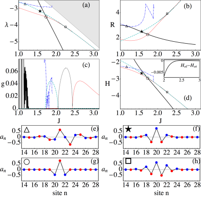
Figure 4: (Color online) Properties of defocusing nonlinear modes: (a) frequency $\lambda$, (b) $R$, (c) stability parameter $g$ and (d) $H$ vs. $J$ for the compact, odd line, odd tip, even line and intermediate modes in thick, thin, dashed, dotdashed and dotted lines, respectively. The linear band in (a) is shown with a shaded area. In the inset of (d) we show the difference between $H$ for the odd line and tip mode. For all non-compact modes $\Gamma=-2.5$. The symbols represent the parameter values of the exemplary modes shown below: (e) $a_{n}$ of the even line mode, (f) $a_{n}$ of the odd tip mode, (g) $a_{n}$ of the odd line mode, (h) $a_{n}$ of the intermediate mode. Red and blue filled circles represent the amplitude at line and tip sites, respectively.

The nonlinear compactons described above are not isolated solutions for a chain with a given $J$, but rather belong to certain families of, generally non-compact, nonlinear localized modes which may be tuned to compactness by varying the effective nonlinearity (e.g., by power tuning) so to fulfill the compacton condition (14). We first illustrate this scenario for an effectively defocusing nonlinearity, $\Gamma<0$, in Fig. 4. The relations of $\lambda$, $R$, $g$ and $H$ vs. $J$, for four families of ordinary localized modes with $\Gamma=-2.5$, in comparison to the compact mode with its respective $\Gamma$ given by (14), are shown in Fig. 4 (a)-(d). Here, the thick (thin, dashed, dotdashed) line represents the compact (odd line, odd tip and even line) mode; some examples for these modes are shown in Figs. 4 (e)-(g), with parameter values corresponding to the respective symbols. The odd line mode is centered at a line site and has the same symmetry as the compacton, while the even line mode, as well as the odd tip mode, have different symmetries being centered around or at a tip site (the even line mode has its main amplitudes at the surrounding line sites, while the odd tip mode is primarily localized at the central tip site). As usual in cubic lattices, the even line mode is unstable everywhere. An example for its profile $a_{n}$ is shown in Fig. 4 (e). We chose parameter values, where its participation number $R$ is very close to the compact mode, but, there is a difference in frequency and Hamiltonian, and the profile shows broader exponential tails. The same happens for the odd tip mode Fig. 4 (f), which is also not directly connected to the compact mode. Finally, the family of odd line modes possesses one compact mode for the specific parameter relation $(\Gamma,\bar{\lambda}_{c},J)$, which is shown in Fig. 4 (g). Thus, the nonlinear compact modes appear as special cases of the continuous family of stable, exponentially localized, modes centered on a line site, which can be tuned to compactification at these specific parameter values.

For larger $J$, the odd line mode has an interval of instability around $2.43\lesssim J\lesssim 5$, where it changes its form (upper bifurcation not shown in Fig. 4(c)). The tip sites next to the central line site grow and pass its amplitude. A similar instability interval appears for the family of odd tip modes for smaller $J$, $1.7\lesssim J\lesssim 2.05$. In the interval between the two bifurcation points where the odd tip modes stabilize and the odd line modes destabilize, a family of intermediate, asymmetric modes appears (cf. Fig. 4(h)). This unstable mode, shown in Fig. 4 with a dotted line in its regime of existence, is responsible for transferring the instability between the odd tip and line modes, and merges with the odd modes at the bifurcation points. In the inset of Fig. 4(d) we show the difference between $H$ for the odd line and tip mode, where the crossing hints at this stability exchange scenario and the existence of the intermediate solution. Note however, that this regime is rather far from the compactification regime.

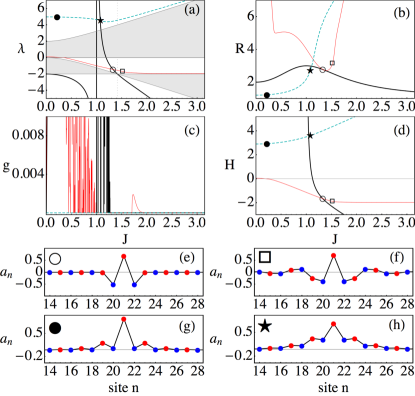
Figure 5: (Color online) Properties of focusing nonlinear modes: (a) frequency $\lambda$, (b) $R$, (c) stability parameter $g$ and (d) $H$ vs. $J$ for the compact mode (thick black), the compactifying odd line gap mode when $\Gamma=1.2$ (thin red), and the non-compactifying odd line mode above the spectrum when $\Gamma=5$ (dashed green). Examples of stable modes are shown below: gap modes in (e)-(f) and modes above the spectrum in (g)-(h).

The analogous compactification of a nonlinear localized, stable gap mode for focusing nonlinearity is illustrated in Fig. 5 (for simplicity, we include in this figure only modes with main peak at a single line site). It is important to stress that the compactifying mode, with its sign changing amplitudes (Fig. 5 (e), (f)) is not identical to the fundamental odd line mode with amplitudes of the same sign (Fig. 5 (g), (h)) and frequency above the spectrum, and they may both exist as simultaneously stable solutions. The condition to have the compactifying mode stable at the point where it compactifies requires the nonlinearity to be relatively weak, $\Gamma\lesssim 2.3$ (cf. (14)). On the other hand, the fundamental odd line mode exists as a stable solution also for larger $\Gamma$, as illustrated in Fig. 5 for $\Gamma=5$, where the compact mode also has a frequency above the linear spectrum but is unstable. The properties of the compactifying modes for stronger focusing nonlinearities will be discussed further for the saturable nonlinearities in Sec. IV (cf. Fig. 8).

IV Saturable nonlinearity

Here, we consider a saturable nonlinearity, taken in equivalent form as in, e.g., Ref. NVS11 and references therein,

$$f(x)=\frac{x}{1+x}\ .$$

Thus, in the small-amplitude limit, the Kerr nonlinearity of Sec. III.1 is reproduced, while saturability effects become important for larger amplitudes. Note in particular that in the large-amplitude, strongly saturated, limit, $f(x)\rightarrow 1$, so the system (1) becomes again effectively linear with just a frequency shift of the linear dispersion relation (II), $\lambda\rightarrow\lambda+\gamma$.

We then obtain for the left-hand side in the general compacton condition (7):

$$\frac{\gamma}{J_{l}}\frac{|A|^{2}(1-1/|J|^{2})}{\left(1+|A|^{2}\right)\left(1+|A/J|^{2}\right)},$$

which gives a second-degree equation for $|A|^{2}$. Solving this and using Eq. (8) gives the following expression for the total compacton power, as function of the coupling ratio $J$ and the rescaled nonlinearity/saturability parameter $\Gamma_{s}\equiv\gamma/J_{l}$:

$$P_{\pm} =\frac{1}{2}\left(1+2/\left|J\right|^{2}\right)\left[\Gamma_{s}\frac{\left|J\right|^{2}-1}{2-J^{2}}-1-\left|J\right|^{2}\right.$$ (16)

$$\pm\left.\sqrt{\left(\Gamma_{s}\frac{\left|J\right|^{2}-1}{2-J^{2}}-1-\left|J\right|^{2}\right)^{2}-4\left|J\right|^{2}}\ \right].\quad$$

It is important to stress that $\Gamma_{s}$ and $P$ act as two independent parameters for the saturable case, in contrast to the pure power-law case from Sec. III which only depends on the combination $(\gamma/J_{l})^{1/\sigma}P$. Thus, a saturable nonlinearity introduces an additional, qualitatively different, mechanism for compactification tuning via the saturability parameter $\Gamma_{s}$.

We can note some general features of the expression (16): for given generic parameter values, there are either zero or two possible solutions with different power (but note of course that only solutions with $P>0$ have physical meaning as compacton solutions). Also, for real $J$, the low power branch $P_{-}$ and the high power branch $P_{+}$ are positive within the same parameter space. Thus, an important difference to the cubic case is that the saturable nonlinearity promotes the appearance of two different compact modes for a given value of $J$, for the same existence regions. These two solutions possess the same profile (equal $\alpha$), but different amplitude $A$.

Bifurcation points, where two solutions coincide, appear when the expression under the square root in (16) is zero, which happens when

$$\gamma_{bif}^{\pm}\equiv\Gamma_{s}=\frac{\left(J^{2}-2\right)\left(1\pm\left|J\right|\right)}{(1\mp|J|)}\ .$$ (17)

For a given $\Gamma_{s}$, this gives a third-degree equation for the coupling ratios $J$ where bifurcations appear. Note, in particular, that when $\Gamma_{s}=-2$, one bifurcation point appears at $J=0$ (with $P\rightarrow\infty$). The consequence is that, in addition to the two branches of solutions continuing the linear solution at $J=\sqrt{2}$, two new branches appear for small $J$ when $\Gamma_{s}<-2$ (see Fig. 6 (c), and lower left parts of (a) and (b)). Note also that at bifurcation points, the power is given by

$$P_{\pm}=\left|J\right|\left(1+2/\left|J\right|^{2}\right),$$

and $|A|^{2}=|J|$.

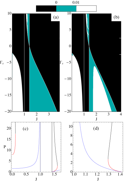
Figure 6: (Color online) Top (a) and (b): white and shaded (green) areas show the existence regimes for exact compactons with saturable nonlinearity where $P>0$ from (16) (black regions imply no solutions). The non-vertical boundaries (white lines) show $\gamma_{bif}^{+}$ from (17). Additionally, we indicate the stability $g$ for (a) $P_{-}$ and (b) $P_{+}$ solutions, where stable solutions are contained in the shaded (green) regions ($g<0.01$), while white regions are unstable ($g>0.01$). Bottom: two examples of power vs. coupling ratio $J$ for $\Gamma_{s}=-2.5$ (c) and $\Gamma_{s}=2.5$ (d). Solid lines show the $P_{-}$ (lower red) and $P_{+}$ (upper black) branches, while dashed blue line shows the corresponding expression for the cubic case (14).

From Fig. 6 we can see the limits of existence (non-black regions in top figures) of the compacton solutions vs. $J$ and $\Gamma_{s}$. For $\Gamma_{s}\leq-2$, there are two windows of existence delimited by $\gamma_{bif}^{+}$ (white line) and $J_{lin}=\sqrt{2}$. For $\Gamma_{s}>-2$, there exists only one region of compactons delimited by $\gamma_{bif}^{+}$ and $J_{lin}=\sqrt{2}$. Two examples for the saturable compacton power (16) as a function of $J$ for $\Gamma_{s}=-2.5$ (c) and $\Gamma_{s}=2.5$ (d) are shown on the bottom of Fig. 6, together with the corresponding expression for the cubic case (14), which only agrees with the saturable case in the small-power regimes, as it should. The region in parameter space of $J$, where the lower saturable compacton branch $P_{-}$ is well approximated by the cubic compactons, increases with increasing $|\Gamma_{s}|$, as exemplified for $\Gamma_{s}=\pm 10$ in the insets of Figs. 7-8 (d). Note however that, in contrast to the cubic case, for each fixed $\Gamma_{s}$ there is always an upper limit for $|J|$ for compacton existence along the branch with $|J|>\sqrt{2}$ bifurcating from the linear compacton when $\Gamma_{s}<0$. This limit, given by $|J_{max}|=J(\gamma_{bif}^{+})$, grows monotonically with $|\Gamma_{s}|$, and it follows from (17) that $|J_{max}|\sim\sqrt{-\Gamma_{s}}$ for large negative $\Gamma_{s}$. Note also that, as $\Gamma_{s}$ decreases towards large negative values, the additional branch for small $J$ born at $\Gamma_{s}=-2$ approaches the branch with $|J|<1$ appearing for $\Gamma<0$ in the cubic case (Sec. III.1). However, in contrast to the cubic case also this branch has an upper limit for $|J|<1$, and it can be seen from (17) that $|J_{max}|\sim 1-2/|\Gamma_{s}|$ for large negative $\Gamma_{s}$. When $\Gamma_{s}>0$, the condition to have $P>0$ demands that compactons may only appear for $|J|<\sqrt{2}$, just as for the cubic case in Sec. III.1. However, as seen in Fig. 6, this solution branch now has a lower limit with $|J|>1$, and from (17) we now obtain $|J_{min}|\sim 1+2/\Gamma_{s}$ for large positive $\Gamma_{s}$.

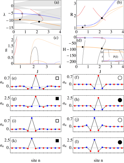
Figure 7: (Color online) Diagrams for saturable nonlinear solutions with defocusing nonlinearity $\Gamma_{s}=-10$. (a) $\lambda$ versus $J$, (b) $R$ versus $J$ (c) $g$ versus $J$, and (d) $H$ versus $J$, with inset $P$ versus $J$. Exact compactons are shown in Red ($P_{-}$) and Black ($P_{+}$) lines, while odd line localized solutions are shown in Blue and Orange for $P=1$ and $P=10$, respectively. Dashed lines correspond to odd tip solutions for same parameters. Profiles for different powers and $J$ (marked by empty and filled squares and circles) are shown for (e)–(h) odd line and (i)–(l) odd tip modes. In (a) the linear ($P\rightarrow 0$, upper two bands) and saturated ($P\rightarrow\infty$, lower two bands) linear band spectra are shown with shaded areas.

Analogously to the studies for the cubic nonlinearity illustrated in Fig. 3, we have analyzed numerically the stability of the two saturable compacton solutions. The results are summarized in Fig. 6 (explicit examples for $\Gamma_{s}=\pm 10$ are shown in Figs. 7-8 (c)). When $\Gamma_{s}<0$ (effectively defocusing nonlinearity) and $J>\sqrt{2}$, the low power ($P_{-}$) branch is, as in the defocusing cubic case, always stable, independent of the $\Gamma_{s}$-value. Decreasing $\Gamma_{s}<0$, the high-power ($P_{+}$) solutions destabilize for intermediate values of $J$, but generally regimes of stable compactons remain for low and high $J$ (the former corresponding to higher power and stronger saturation). Thus, for defocusing saturable nonlinearities two different stable compacton modes with different powers, having similar profiles (equal value of $R$) may exist for a given $\Gamma_{s}$. Fig. 6 also shows that both solutions appearing for $J<1$ when $\Gamma_{s}<-2$ always are unstable. Similarly to the cubic case, this regime is not connected with flat-band linear modes. When $\Gamma_{s}>0$ (effectively focusing nonlinearity), a similar scenario as in the focusing cubic case is observed for the compact mode continued from the linear limit at $J=\sqrt{2}$: it is stable for small powers but destabilizes through resonances with extended lattice modes for larger powers. However, similarly to the defocusing saturable case, the compact mode generally restabilizes in the strongly saturated, high-power regime of the $P_{+}$ branch, and thus we may also for the focusing case find regimes of two simultaneously stable compactons, although only in a narrow interval for $J\lesssim\sqrt{2}$.

To study the relation of these compact solutions with families of standard, non-compact, localized modes (cf. Fig. 4 for the cubic case), we first present in Fig. 7 collected results for $\Gamma_{s}=-10$, i.e., an effectively defocusing case with two different regions for analytical solutions. First, as discussed above, compact solutions are seen to bifurcate at $J=\sqrt{2}$ from linear flat band modes with zero ($P_{-}$) and infinite ($P_{+}$) power, coinciding with the low and high amplitude (saturated) linear spectra (the latter being shifted to $\lambda+\gamma$ due to saturation) as shown in Fig. 7(a). For $J>\sqrt{2}$, we see that both $P_{-}$ and $P_{+}$ compacton branches (but not the branches with $J<1$) appear as compactifications of families of standard localized modes with main localization at the central line site. Analogously to the cubic case in Sec. III.1, we illustrate in Fig. 7 properties of numerically obtained families of modes centered at line and tip sites, respectively, at two different fixed values of power: $P=1$ and $P=10$. Figs. 7(e)–(l) show profiles for low power solutions (empty squares and empty circles) and high power ones (black squares and black circles), for different values of $J$ as well as for line and tip site centers. Note that, while the low-power compactifying line-site centered mode (Figs. 7(e)–(f)) is always stable for the relevant regime in $J$, just as in the cubic case, the corresponding family of high-power modes for $P=10$ (Figs. 7(g)–(h)) has an instability window around the compactification point, and thus this compact mode is unstable. This instability window moves as the power is further increased, implying that, as mentioned above, also the high-power compacton branch stabilizes for a sufficiently high power (for $\Gamma_{s}=-10$, high-power compacton restabilization appears for $P\gtrsim 25.36$, corresponding to $J\lesssim 1.75$). Note that also the non-compact modes with exponential tails are strongly localized (small $R$) for these parameter values, as they are residing far below the linear band.

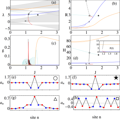
Figure 8: (Color online) Diagrams for saturable nonlinear solutions with focusing nonlinearity, $\Gamma_{s}=10$. (a)-(d) show the same quantitites as Fig. 7 (a)-(d) with the same line coding for solutions. In addition, compactifying odd line localized solutions are shown in black dotdashed for $P=1$ and green dotted for $P=10$. Profiles at positions indicated by markers: (e), (f) modes from the compactifying family at $P=10$ (localized modes above linear spectrum); (g) the fundamental (noncompactifying) stable odd line mode at $P=1$; (h) mode from the compactifying family at $P=1$ (non-localized mode inside upper linear band). Shaded areas in (a) represent dispersion bands in the linear ($P\rightarrow 0$, lower two bands) and saturated ($P\rightarrow\infty$, upper two bands) limits.

In Fig. 8, we illustrate in an analogous way the case with focusing nonlinearity, $\Gamma_{s}=+10$. As in the cubic case, neither the upper nor lower compacton branches then appear as compactifications of the family of fundamental localized modes with constant sign and main localization at the central line site, which is seen to appear simultaneously as a stable solution but with different properties (Fig. 8 (g)). For small powers, when the compacton frequency is still in the linear gap, the scenario is similar to the cubic case illustrated in Fig. 5 with a compactifying gap mode with a tail of oscillating signs (cf. Fig. 5 (f)). For slightly larger powers ($P=1$ in Fig. 8), when the compacton frequency has entered the upper linear band but still belongs to the $P_{-}$ compacton branch, the compactifying family is not localized but has a non-decaying, oscillating tail (Fig. 8 (h)), which vanishes only at the compactification point. As seen in Fig. 8 (c), these solutions are generally unstable. Finally, when the power is large enough for the compacton frequency to reside above the linear spectrum (belonging then to the $P_{+}$ branch for the case in Fig. 8 (a)), the compactifying family is again a localized solution with main localization at three sites, where only the central site has a different amplitude sign than the other sites (Fig. 8 (f)). From Fig. 8 (c), this solution is seen to be stable in parts of its existence regime (e.g., the mode in (f)), but for these parameter values, it is unstable at the point where it compactifies. However, for even larger $P$, at strong saturation, these solutions will also be stable at the compactification point, as illustrated in Fig. 6 (b). This restabilization of the compactifying focusing mode above the linear spectrum at high power is another characteristic feature of the saturable system, which does not appear for the cubic case.

V Further tuning options

Let us now consider a generalization of Eq. (1), by adding a non-homogeneous distribution $\Delta_{n}$ of on-site energies, and allowing also for anisotropies in the coupling coefficients $J_{n,m}$,

$$i\dot{u}_{n}+\Delta_{n}u_{n}+\sum_{m}J_{n,m}u_{m}+\gamma f(|u_{n}|^{2})u_{n}=0.$$ (18)

We were able to find three-site compact modes, having the same symmetric line-site centered structure as described in Sec. II, for a distribution of

$$\Delta_{n}/J_{l}=\begin{cases}0&\text{ for $n$ odd}\\ \Delta&\text{ for $n$ even.}\end{cases}$$ (19)

This means, that the tips have an on-site energy of $\Delta$, whereas the line sites have vanishing on-site energy (the linear dispersion relation and the corresponding linear compact mode in the isotropic sawtooth lattice with $\Delta=-1$ were illustrated in Ref. Flach14 , Fig. 1 (f)).

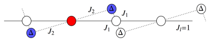
Figure 9: (Color online) Sketch of the anisotropic geometry with pairwise alternating couplings and alternating on-site energies.

Considering also various ways to introduce coupling anisotropies in the sawtooth lattice, one possibility would be to have constant line coupling with alternating couplings to the tips. However, such a structure only allows for asymmetric linear compactons for some specific ratio of the two tip coupling constants, and no compact nonlinear continuations were found for these modes for any distribution of on-site energies of the type (19) with identical tip energies (nonlinear asymmetric compactons may exist under special conditions if the alternating coupling is also combined with different on-site energies for up- and down- pointing tip sites, but these conditions are more complex and will not be discussed further here). On the other hand, a nonlinear continuation of symmetric compact modes is possible, if instead a pairwise (real) alternating coupling $J_{1}$ and $J_{2}$ is assumed in the tips, as sketched in Fig. 9. Within the line we conserve the coupling $J_{l}=1$. In this case, the four linear bands are given by

$$\lambda_{\pm,\pm}=\frac{\Delta}{2}+\cos(2k)\pm$$ (20)

$$\sqrt{(J_{1}^{2}+J_{2}^{2})+\left(\frac{\Delta}{2}-\cos(2k)\right)^{2}\pm f_{J_{1},J_{2}}(k)}$$

with

$$f_{J_{1},J_{2}}(k)=\sqrt{J_{1}^{4}+J_{2}^{4}-2J_{1}^{2}J_{2}^{2}+4J_{1}^{2}J_{2}^{2}\cos^{2}(2k)}$$

The geometry allows for two different types of compact modes, one that has the line site coupled to the tips with $J_{1}$, the other with $J_{2}$. Without loss of generality we will consider only the latter, shown exemplary in Fig. 9. For a Kerr nonlinearity, the symmetric compact modes with amplitude ratio $\alpha=-1/J_{1}$ appear when the following conditions for the effective nonlinearity (14) and frequency are fulfilled,

$$\Gamma_{\Delta}(J_{1},J_{2}) = \frac{J_{2}(J_{1}^{4}-4)-J_{1}\Delta(J_{1}^{2}+2)}{J_{1}-J_{1}^{3}}$$

$$\lambda_{\Delta} = \frac{\Delta J_{1}^{3}+2J_{2}-J_{1}^{4}J_{2}}{J_{1}^{3}-J_{1}}$$

V.1 Alternating on-site energies

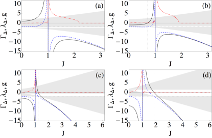
Figure 10: (Color online) Compact mode $\Gamma_{\Delta}$ (solid), $\lambda_{\Delta}$ (dashed), and stability parameter $g$ (dotted) vs. $J$ for $\Delta=-2.5$ (-1.5,-0.5, 1.5) in (a)-(d). The shaded areas denote the band extensions.

We first turn to the isotropic case of $J_{1}=J_{2}=J$, but $\Delta\neq 0$. The linear dispersion relation (20) for this case is

$$\lambda_{\pm}(k) = \frac{\Delta}{2}+\cos(2k)\pm$$

$$\sqrt{\left(\cos(2k)-\frac{\Delta}{2}\right)^{2}+2J^{2}[1+\cos(2k)]},$$

whereas the Eqs. (LABEL:compdeltaj1j2) simplify to

$$\Gamma_{\Delta} = \frac{\left(J^{2}+2\right)\left(J^{2}-\Delta-2\right)}{1-J^{2}}$$

$$\lambda_{\Delta} = \frac{\Delta J^{2}+2-J^{4}}{J^{2}-1}.$$

This gives a linear compact mode for $J_{\Delta,lin}=\sqrt{2+\Delta}$, thus there is only a continuation of the linear compact solution for $\Delta\geq-2$. The bandgap vanishes as well for $\Delta=-2$. However, nonlinear compact solutions exist also for $\Delta<-2$. In Fig. 10 we show different scenarios. For $\Delta=-2.5$ (see Fig. 10(a)), there is no flat band and the compact mode does not cross the bandgap. For $\Delta=-1.5$ (see Fig. 10(b)), the flat band is located for $J<1$, where the compacton frequency curve enters and crosses the bandgap with positive $\Gamma_{\Delta}$. The sign of the discontinuity at $J=1$ changes at $\Delta=-1$ and with it the location of the flat band, so for $\Delta=-0.5$ and $\Delta=1.5$ (Fig. 10(c)-(d)) the crossing of the bandgap is found for $J>1$. Increasing $\Delta$ further only opens the gap more, but there will be no further changes in regarding the bandgap. Therefore, the on-site energy difference $\Delta$ gives rise to the possibility of a direct engineering of the bandgap as well as the nonlinearity and frequency of the compacton.

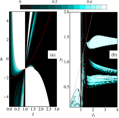
Figure 11: (Color online) Stability parameter $g$ of the compact mode vs. $J_{1}=J_{2}=J$ and $\Delta$ (a), vs. $J_{1}$ and $J_{2}$ with $\Delta=0$ (b), only the black areas ($g<0.05)$ contain stable modes. $N=40$. In (a) compactons are unstable also in the black stripe for small $J$ when $\Delta>-2$, but have $g<0.05$. The linear compacton condition is given by red lines, the ordinary sawtooth with homogeneous $J_{2}=J_{1}$ is marked with a gray line.

The stability for compact modes vs. $J$ and $\Delta$ are shown with dotted lines for the specific examples in Figs. 10(a)-(d). The general stability scenario is explored in Fig. 11(a), where black areas denote stable or weakly unstable ($g<0.05$) compactons and the degree of instability increases with brightness. As a guide to the eye, we denote the parameters of the linear compacton, $\Delta=\sqrt{J^{2}-2}$, with a red line. This line apparently separates two different regimes, with the main lobes of the instability located at opposite sides of $J=1$. For a fixed $\Delta<-2$ (Fig. 10 (a)), there is always a stable regime for small $J$, corresponding to a compacton with main amplitude at the tip sites in a chain with focusing nonlinearity. For growing $J$, some weaker instabilities are passed for $J<1$, and at $J=1$ the large instability lobe appears as the compacton now exists for defocusing nonlinearity. By comparing with the stability results for the corresponding solutions in the open trimer configuration (without a surrounding lattice) Buonsante , it can be deduced that the instabilities on the focusing side ($J<1$) are due to resonances with lattice oscillations (since this regime is always stable for the trimer Buonsante ), while on the defocusing side ($J>1$) it is an internal resonance in the compacton core which appears also for the trimer. In the regime $-2<\Delta<-1$ (Fig. 10 (b)), the main qualitative change appears in the small-$J$ regime, where the nonlinearity now is defocusing for $J<J_{\Delta,lin}$ and the compacton is unstable. In fact, if follows from analogous considerations for the open trimer Buonsante that compactons with main localization on tip sites (small $J$) are always unstable through core instabilities for defocusing nonlinearities. For $\Delta>-1$ (Fig. 10 (c)-(d)), the mode is always unstable in the defocusing regime $0<J<1$. When $\Delta\gtrsim-1$, we also see an instability in the other defocusing region for $J>J_{\Delta,lin}$, as a remains of the instability lobe at $J>1$ for smaller $\Delta$. For larger $\Delta$, these instabilities disappear and the only significant instabilities observed for $J>1$ are those in the focusing regime $J<J_{\Delta,lin}$, which are analogous to those described for the homogeneous case $\Delta=0$ in Sec. III.1. In general, for all $\Delta$ the compacton always approaches a stable one-site line-mode for large $J$, corresponding to a strong defocusing Kerr nonlinearity.

One important conclusion from the above analysis is, that by introducing alternating on-site energies with $\Delta<-2$ one may, for focusing nonlinearity, stabililize also compactons with main localization at the tip sites, which in the previous Sections were found to be always unstable for the homogeneous sawtooth lattice.

V.2 Pairwise alternating couplings

We finally turn briefly to the case of pairwise alternating coupling as in Fig. 9, but considering for simplicity only vanishing on-site energies $\Delta=0$. As the linear stability analysis vs. $J_{1}$ and $J_{2}$ for this family shows (see Fig. 11(b)), for small external coupling to the array $J_{1}\leq 1$ (corresponding to defocusing nonlinearity, $\Gamma<0$ according to (LABEL:compdeltaj1j2)) nearly all modes (having their main amplitudes on tip sites) are unstable, only a very restricted zone for small $J_{2}<J_{1}$ is stable. On the other hand, if $J_{1}>1$, there are as before many regimes of stable modes. In the focusing regime, $1<J_{1}<\sqrt{2}$ (see (LABEL:compdeltaj1j2)), the stability scenario is qualitatively similar as for the case $J_{2}=J_{1}$ described in Sec. III.1; changing the internal coupling $J_{2}$ mainly changes the internal compacton oscillation frequencies and thereby also the exact location of the instability threshold resulting from their resonances with the surrounding chain, but a stable regime generally remains for small nonlinearity. In the defocusing regime $J_{1}>\sqrt{2}$, the compacton having main amplitude on the line-site always remains stable for $J_{2}\geq J_{1}$, but it may destabilize in certain regimes for $J_{2}<J_{1}$, i.e., when the internal coupling is weaker than the external. Note in particular the instability window around $J_{2}=\sqrt{2}$, corresponding to a resonance with a linear compacton with internal coupling $J_{1}$.

VI Conclusions

In this work we showed the existence of compact modes for generic realizations of the sawtooth lattice, considering power law and saturable nonlinearities. These modes are compact nonlinear continuations of the linear flat-band modes found in the sawtooth model. For a wide window in parameter space we showed the stability of these modes for both focusing and defocusing nonlinearities. Furthermore, we explored the influence of inhomogeneous on-site energies and pairwise alternating coupling on the band-structure and stability of the compact modes. We observed, that negative on-site energies or high anisotropic pairwise coupling increase the stability regimes.

Moreover, we have confirmed the existence of compacton solutions for the saturable nonlinearity, finding stable regimes for two types of analytical solutions. As they are very compact solutions, they could be easily excited in an experiment, for low level of power and for different sawtooth geometries governed by the coupling ratio $J$. The possibility to excite very localized nonlinear solutions using low level of power is an important property of this particular lattice, in contrast with nonlinear conventional lattices VJ13 . We also found regimes with possibility to excite two, simultaneously stable, compactons with similar profiles, for small and large level of power. This is a very interesting property of the sawtooth lattice; in conventional systems, stable solutions for different level of power exist but with different profile structure (e.g., different participation number).

- (1) S. Flach and A.V. Gorbach, Phys. Rep. 467, 1 (2008).
- (2) F. Lederer, G.I. Stegeman, D.N. Christodoulides, G. Assanto, M. Segev, and Y. Silberberg, Phys. Rep. 463, 1 (2008).
- (3) P.G. Kevrekidis and V.V. Konotop, Phys. Rev. E65, 066614 (2002); P.G. Kevrekidis, V.V. Konotop, A.R. Bishop, and S. Takeno, J. Phys. A: Math. Gen. 35, L641 (2002).
- (4) M. Öster, M. Johansson, and A. Eriksson, Phys. Rev. E67, 056606 (2003); M. Öster and M. Johansson, Phys. Rev. E71, 025601(R) (2005); Physica D 238, 88 (2009).
- (5) F.Kh. Abdullaev, P.G. Kevrekidis, and M. Salerno, Phys. Rev. Lett. 105, 113901 (2010).
- (6) O. Derzhko, J. Richter, A. Honecker, M. Maksymenko, and R. Moessner, Phys. Rev. B81, 014421 (2010).
- (7) S.D. Huber and E. Altman, Phys. Rev. B82, 184502 (2010).
- (8) S. Flach, D. Leykam, J.D. Bodyfelt, P. Matthies, and A.S. Desyatnikov, EPL 105, 30001 (2014).
- (9) Z. Liu, F. Liu, and Y.-S. Wu, Chin. Phys. B 23, 077308 (2014).
- (10) D. Guzmán-Silva, C. Mejía-Cortés, M.A. Bandres, M.C. Rechtsman, S. Weimann, S. Nolte, M. Segev, A. Szameit and R.A. Vicencio, New J. Phys. 16, 063061 (2014).
- (11) R.A. Vicencio, C. Cantillano, L. Morales-Inostroza, B. Real, C. Mejía-Cortés, S. Weimann, A. Szameit and M.I. Molina, Phys. Rev. Lett. 114, 245503 (2015).
- (12) S. Mukherjee, A. Spracklen, D. Choudhury, N. Goldman, P. Öhberg, E. Andersson, and R.R. Thomson, Phys. Rev. Lett. 114, 245504 (2015).
- (13) D.L. Bergman, C. Wu, and L. Balents, Phys. Rev. B78, 125104 (2008).
- (14) R.A. Vicencio and M. Johansson, Phys. Rev. A87, 061803(R) (2013).
- (15) D. Sen, B.S. Shastry, R.E. Walstedt, and R. Cava, Phys. Rev. B53, 6401 (1996).
- (16) J. Schulenburg, A. Honecker, J. Schnack, J. Richter, and H.-J. Schmidt, Phys. Rev. Lett. 88, 167207 (2002).
- (17) M.E. Zhitomirsky and H. Tsunetsugu, Phys. Rev. B70, 100403(R) (2004).
- (18) T. Nakamura and K. Kubo, Phys. Rev. B53, 6393 (1996).
- (19) M. Hyrkäs, V. Apaja, and M. Manninen, Phys. Rev. A87, 023614 (2013).
- (20) S. Weimann, Y. Xu, R. Keil, A.E. Miroshnichenko, A. Tünnermann, S. Nolte, A.A. Sukhorukov, A. Szameit, and Y.S. Kivshar, Phys. Rev. Lett. 111, 240403 (2013).
- (21) R.A. Vicencio and A. Szameit, in Advanced Photonics, OSA Technical Digest (Optical Society of America, Washington, DC, 2014), paper JTu3A.59.
- (22) S. Rojas-Rojas, L. Morales-Inostroza, U. Naether, G.B. Xavier, S. Nolte, A. Szameit, R.A. Vicencio, G. Lima, and A. Delgado, Phys. Rev. A90, 063823 (2014).
- (23) A. Khare, K.Ø. Rasmussen, M.R. Samuelsen, and A. Saxena, J. Phys. A: Math. Gen. 38, 807 (2005).
- (24) C. Schmidt-Hattenberger, R. Muschall, U. Trutschel, and F. Lederer, Opt. Quantum Electron. 24, 691 (1992).
- (25) U. Naether, R.A. Vicencio, and M. Stepić, Opt. Lett. 36, 1467 (2011).
- (26) P. Buonsante, R. Franzosi, and V. Penna, Phys. Rev. Lett. 90, 050404 (2003); J. Phys. A: Math. Theor. 42, 285307 (2009).