Geodesic acoustic modes in a fluid model of tokamak plasma : the effects of finite beta and collisionality

Abstract

Starting from the Braginskii equations, relevant for the tokamak edge region, a complete set of nonlinear equations for the geodesic acoustic modes (GAM) has been derived which includes collisionality, plasma beta and external sources of particle, momentum and heat. Local linear analysis shows that the GAM frequency increases with collisionality at low radial wave number $k_{r}$ and decreases at high $k_{r}$. GAM frequency also decreases with plasma beta. Radial profiles of GAM frequency for two Tore Supra shots, which were part of a collisionality scan, are compared with these calculations. Discrepency between experiment and theory is observed, which seems to be explained by a finite $k_{r}$ for the GAM when flux surface averaged density $\langle n\rangle$ and temperature $\langle T\rangle$ are assumed to vanish. It is shown that this agreement is incidental and self-consistent inclusion of $\langle n\rangle$ and $\langle T\rangle$ responses enhances the disagreement more with $k_{r}$ at high $k_{r}$ . So the discrepancy between the linear GAM calculation, (which persist also for more “complete” linear models such as gyrokinetics) can probably not be resolved by simply adding a finite $k_{r}$.

I Introduction

Common wisdom in fusion plasma science is that the transport of heat and particles in tokamaks are largely due to micro-turbulence driven by background gradients of density, temperature, momentum etc. The turbulence saturates via mode coupling, and in particular by interactions with self-generated large scale flow structures such as zonal flows(diamond, ),and in some cases, especially near the edge, with geodesic acoustic modes (GAMs)(winsor:68, ; miki:2007, ; miki:2008, ). GAMs are an important class of oscillating zonal flows that appear due to toroidal geometry (i.e. due to geodesic curvature), and are easily observable in tokamak experiments due to their finite frequency. They are usually classified as an $m=n=0$ perturbation in potential coupled with an $m=1$, $n=0$ perturbation in density or pressure, where $m$ and $n$ are the poloidal and the toroidal mode numbers respectively. GAMs are linearly damped unless fast particles are present(fu:2008, ; fu:2011, ; qiu:2010, ; qiu:2012, ; zarzoso:2012, ; wang:2014, ; girardo:2014, ). Otherwise they are excited by nonlinear processes like turbulent reynolds stresses(nikhil:2007, ; nikhil:2008, ; guzdar:2008, ; zonca:epl2008, ; guzdar:2009, ; yu:2013, ; chen:2014, ), poloidally asymmetric particle fluxes(itoh:2005, ) and heat fluxes(hallatschek:2001, ). Due to their finite frequency (usually a few $kHz$), distinct from that of broadband turbulence, GAMs are easier to detect, and thus have been observed on several tokamaks such as ASDEX Upgrade (AUG) (conway:05, ) using Doppler backscattering (DBS), TEXTOR (flecken:2006, )using O-mode correlation reflectometer, and DIIID (mckee:06, ) using beam emission spectroscopy (BES). As of today, GAMS are observed in the majority of the tokamaks in the world including recent observations of GAMs in Tore Supra (vermare:12, ) using a DBS system. The common aspect of these measurements is that the GAMs are most prominent in the edge region, right inside the last closed flux surface, and extend into the near edge region (sometimes called the no man’s land due to a seemingly systematic discrepency between simulation and experiment (holland:09, )). While gyrokinetics is accepted widely as the most general formulation for strongly magnetised plasmas of tokamak fusion devices, the applicability of gyrokinetic vs. fluids models is still somewhat open to debate in the edge region. For most existing tokamaks, as one goes from the core to the edge, the collisions start to play a role, and the parallel connection length increases (since the safety factor $q$ increases), dissipative drift waves, or resistive balloning modes, start to become important, therefore the validity of a fluid description including the effects of collisions may actually be justified(rafiq:10, ; militello:11, ).

In this spirit, here we will develop a simple two fluid model for the description of the GAM, using Braginskii equations (braginskii:65, ; zeiler:97, ) within a drift expansion, in order to include the effects of collisions. In particular we include equations of contunity, momentum and heat for ions and electrons (i.e. using a generalized Ohm’s law for electrons) coupled with the Ampère’s law. The formulation allows us to include $v_{\parallel}$, $A_{\parallel}$, $T_{i}$ and $T_{e}$ perturbations of the GAM in a full set of nonlinear equations, which can be linearized and solved to obtain the GAM frequency including the effects of collisions and finite $\beta$, and finite radial mode number $k_{r}$.

The computed frequency is then compared with the radial profile of GAM frequency that is observed in Tore Supra during a collisionality scan (assuming $k_{r}\approx 0$). There is an apparent, systematic discrepancy between the theory and the experiment, which seems to be explained when a finite $k_{r}$ is introduced for the GAM calculation assuming flux surface averaged density $\langle n\rangle$, ion temperature $\langle T_{i}\rangle$ and flux surface averaged electron temperature $\langle T_{e}\rangle$ to be zero. However we believe that this agreement is incidental since it breaks down when higher harmonics ($m=2$ etc.) are included in the calculation(nguyen:2008, ; rameswar1:2014, ). The agreement also breaks down on self consistent inclusion of $\langle n\rangle$, $\langle T_{i,e}\rangle$ responses on the GAM dispersion for $m=1$. This indicates that the discrepancy between the linear GAM calculation and the experiment, which persist also for more “complete” linear models such as gyrokinetics, is probably significant and can not be resolved by simply adding a finite $k_{r}$.

The remainder of this paper is organized as follows. The complete set of nonlinear electromagnetic equations with collisionality are obtained in SectionII from the drift reduction of Braginskii equations. The fully nonlinear equations for GAMs are obtained in SectionIII by taking appropriate flux surface averagings of the drift reduced electron and ion equations. Linear GAM dispersion properties are obtained in SectionIII.1 and comparison with experimental data are presented in SectionIII.2. Finally the paper is concluded in SectionIV.

II NONLINEAR MODEL EQUATIONS

In order to formulate the nonlinear theory of electromagnetic geodesic acoustic modes (GAMs), we start with the simple two fluid Braginskii equations(braginskii:65, ; zeiler:97, ), where we keep the following: (i) the non adiabatic electron response with $\delta T_{e}\neq 0$ , and the electron-ion collisionality $\nu_{ei}$. The model equations for GAMs are then derived from the density, momentum and temperature equations for each species $j(=i,e)$.

$$\frac{\partial n_{j}}{\partial t}+\vec{\nabla}\cdot(n_{j}\vec{v}_{j})=0$$ (1)

$$m_{i}n_{i}\left(\frac{\partial v_{i}}{\partial t}+\vec{v}_{i}\cdot\vec{\nabla}\right)v_{i}=-\vec{\nabla}p_{i}-\vec{\nabla}\cdot\bar{\bar{\pi_{i}}}+e\left(\vec{E}+\frac{1}{c}\vec{v}_{i}\times\vec{B}\right)+\vec{R}_{ie}$$ (2)

$$0=-\vec{\nabla}p_{e}-e\left(\vec{E}+\frac{1}{c}\vec{v}_{e}\times\vec{B}\right)+\vec{R}_{ei}$$ (3)

$$\frac{3}{2}n_{j}\left(\frac{\partial}{\partial t}+\vec{v}_{j}\cdot\vec{\nabla}\right)T_{j}+p_{j}\,\vec{\nabla}\cdot\vec{v}_{j}=-\vec{\nabla}\cdot\vec{q}_{j}$$ (4)

where

$$q_{j}=0.71nT_{j}\vec{U}_{||}-\kappa_{||}\nabla_{||}T_{j}+\kappa_{\perp}\nabla_{\perp}T_{j}+q_{*j}+\frac{3}{2}\nu_{j}\frac{nT_{j}}{\omega_{cj}}\hat{b}\times\vec{U}$$ (5)

Here the mass of the electron is neglected and $\vec{E}=\vec{\nabla}\phi-(1/c)\partial{\vec{A}}/\partial{t}$. The collisional momentum transfer term is given by $\vec{R}_{ei}=-\vec{R}_{ie}=ne\eta_{||}\vec{J}_{||}-0.71n\vec{\nabla}_{||}T_{e}$, where $J_{||}=en(v_{i}-v_{||e})$, and $\vec{U}$ is the relative velocity between species $j$ and $i$. The thermal conductivities for electrons are given by $\kappa_{||e}=3.16n_{e}T_{e}/m_{e}\nu_{e}$, $\kappa_{\perp e}=4.66n_{e}T_{e}\nu_{e}/m_{e}\omega_{ce}^{2}$ and for ions $\kappa_{||i}=3.9n_{i}T_{i}/m_{i}\nu_{i}$, $\kappa_{\perp i}=2n_{i}T_{i}\nu_{i}/m_{i}\omega_{ci}^{2}$. The diamagnetic heat flux is taken as $q_{*j}=\frac{5}{2}\frac{p_{j}}{m_{j}\omega_{cj}}\hat{b}\times\vec{\nabla}T_{j}$.

In order to develop a drift expansion, we consider ion and electron perpendicular drift velocities in the low frequency regime ($\omega<<\omega_{ci}$, $\nu_{ei}<<\omega_{ci}$; $\omega$, $\omega_{ci}=eB/m_{i}c$ mode frequency, ion cyclotron frequency, respectively). These drift velocities consist of the$\vec{E}\times\vec{B}$ drift, the ion and the electron diamagnetic drifts, the ion polarization drift:

$$\vec{v}_{E}=(c/B^{2})\vec{B}\times\vec{\nabla}\delta\phi$$ (6)

$$\vec{v}_{*pi}=(c/en_{i}B^{2})\vec{B}\times\vec{\nabla}\delta p_{i}$$ (7)

$$\vec{v}_{*pe}=-(c/en_{e}B^{2})\vec{B}\times\vec{\nabla}\delta p_{e}$$ (8)

$$\vec{v}_{pi}=-\frac{c}{B\omega_{ci}}\left(\frac{\partial}{\partial t}+(\vec{v}_{E}+\vec{v}_{*pi})\cdot\vec{\nabla}\right)\vec{\nabla}_{\bot}\delta\phi$$ (9)

For the equilibrium scale lengths that are larger than the perturbation scales (i.e.,$k_{\bot}L<1$), we can separate the equilibrium ($f_{0}$) and the fluctuating parts ($\delta f$) in the above set of equations as $f=f_{0}+\delta f$. The complete set of resulting reduced nonlinear equations for the perturbations ($\delta f$) are provided in the next subsection which is written in the following normalization scheme. The space time scales are normalized as $r=r/\rho_{s}$, $\nabla_{\parallel}\equiv L_{n}\nabla_{\parallel}$, $t=tc_{s}/{L_{n}}$. The field quantities are normalized to their mixing length levels: $\phi=({e\delta\phi}/{T_{e}})({L_{n}}/{\rho_{s}})$, $n_{i}=({\delta n_{i}}/n_{0})({L_{n}}/{\rho_{s}})$, $v=({\delta v_{\parallel i}}/{c_{s}})({L_{n}}/{\rho_{s}})$, $p_{i}=({\delta p_{i}}/{P_{e0}})({L_{n}}/{\rho_{s}})$, $A_{||}=(2L_{n}c_{s}/\beta\rho_{s}c)(e\delta A_{||}/T_{e0})$. The remaining dimensionless parameters are : $\eta_{i}=L_{n_{i0}}/L_{T_{i0}}$, $K=\tau_{i}(1+\eta_{i})$, $\tau_{i}=T_{i0}/T_{e0}$, $\beta=8\pi P_{0e}/B_{0}^{2}$, $L_{f}=-\,\mathrm{d}lnf/\,\mathrm{d}x$, $\eta_{e}=L_{n_{e0}}/L_{T_{e0}}$, $\nu=0.51m_{e}\nu_{ei}L_{n}/m_{i}c_{s}$. The electron ion collision frequency is calculated from $\nu_{ei}=nZ^{2}ln\lambda/(1.09\times 10^{16}T_{e}^{3/2})$ where $ln\lambda=15.2-log(n/10^{20})+log(T_{e})$(wesson:97, ). $\rho_{s}=c_{s}/\omega_{ci}$ is the ion sound radius. The nonlinearities in the following equations originate mainly from the $E\times B$ drift nonlinearity i.e., $\vec{v}_{E\times B}\cdot\vec{\nabla}f=\left[\phi,f\right]$, the polariztion drift nonlinearity $\vec{v}_{E\times B}\cdot\vec{\nabla}\nabla_{\perp}^{2}f=\left[\phi,\nabla_{\perp}^{2}f\right]$ and the nonlinearity due to the parallel gradients with fluctuating magnetic fields, from $\nabla_{||}=\nabla_{||}^{0}+\tilde{\delta\vec{B}}_{\perp}\cdot\vec{\nabla}=\nabla_{||}^{0}-(\beta/2)\left[A_{||},\quad\right]$, $\nabla_{||}^{0}$ being derivative along the equilibrium magnetic field. The $\beta$ effects enter via perpendicular magnetic field line bending effect through the expressions for $E_{\parallel}$ and the instantaneous parallel derivative.

Such models has also been used for edge turbulence simulations in the references(ricci:2010, ; beyer:1998, ; naulin:2005, ; bdscott:2005, ; Dudson:2009, )

II.1 Electron response

When the drift expansion is considered in toroidal geometry, the electron continuity equation for density perturbation takes the form:

$$\frac{\partial n_{e}}{\partial t}+\frac{1}{r}\frac{\partial\phi}{\partial\theta}-\varepsilon_{n}(\cos\theta\frac{1}{r}\frac{\partial}{\partial\theta}+\sin\theta\frac{\partial}{\partial r})(\phi-n_{e}-T_{e})-\nabla_{||}\left(J_{||}-v_{||}\right)$$

$$=\left[\phi,n_{e}\right]-\frac{\beta}{2}\left[A_{||},J_{||}-v_{||}\right]$$ (10)

These and the following equations has been derived assuming large aspect ratio curcular flux surfaces. The second and third terms in the above equation results from the $E\times B$ convection of equilibrium density, the sum of divergence of $E\times B$ diamagnetic drifts due to inhomogenous magnetic fields of the tokamak, respectively. The first term on the right hand is the $E\times B$ convective nonlinearity and the second term results from parallel derivative nonlinearity due to perpendicular magnetic fluctuations. In the limit $\omega<<k_{||}c_{s}$ the perturbed parallel momentum equation for electrons reads:

$$\nu J_{||}=-\nabla_{||}\left(\phi-n_{e}-1.71T_{e}\right)-\frac{\beta}{2}\left[\frac{\partial}{\partial t}+\left(1+1.71\eta_{e}\right)\frac{1}{r}\frac{\partial}{\partial\theta}\right]A_{||}+\frac{\beta}{2}\left[A_{||},\phi-n_{e}-1.71T_{e}\right]$$ (11)

Similarly, the electron temperature perturbation equation, in the same expansion, becomes:

$$\frac{\partial}{\partial t}(T_{e}-\frac{2}{3}n_{e})+\frac{5}{3}\varepsilon_{n}(\cos\theta\frac{1}{r}\frac{\partial}{\partial\theta}+\sin\theta\frac{\partial}{\partial r})T_{e}+\left(\eta_{e}-\frac{2}{3}\right)\frac{1}{r}\frac{\partial\phi}{\partial\theta}-\frac{1.07}{\nu}\nabla_{||}^{2}T_{e}$$

$$=-\left[\phi,T_{e}-\frac{2}{3}n{e}\right]+\frac{1.07}{\nu}\left\{\nabla_{||}\left(-\eta_{e}\frac{\beta}{2r}\frac{\partial A_{||}}{\partial\theta}-\frac{\beta}{2}\left[A_{||},T_{e}\right]\right)-\frac{\beta}{2}\left[A_{||},\nabla_{||}T_{e}\right.\right.$$

$$\left.\left.-\eta_{e}\frac{\beta}{2r}\frac{\partial A_{||}}{\partial\theta}-\frac{\beta}{2}\left[A_{||},T_{e}\right]\right]\right\}$$ (12)

The first term on the right hand side is the $E\times B$ convective nonlinearity and the second term results from $\tilde{\delta\vec{B}}_{\perp}$part of the parallel derivative. This equation has been derived using the continuity equation for $\nabla\cdot\vec{v}$ and the diamagnetic heat flux cancelation.

Finally, the $J_{||}$ is related to the parallel vector potential $A_{\parallel}$ via the Ampères law:

$$J_{||}=-\nabla_{\perp}^{2}A_{||}$$ (13)

II.2 Ion response

The equations for the ion dynamics can similarly be obtained from the two fluid Braginskii equations using the drift expansion, with the aforementioned assumptions. The resulting equation for the continuity of ions take the form:

$$\frac{\partial n_{i}}{\partial t}+\frac{1}{r}\frac{\partial\phi}{\partial\theta}-\epsilon_{n}\left(\cos\theta\frac{1}{r}\frac{\partial}{\partial\theta}+\sin\theta\frac{\partial}{\partial r}\right)\left(\phi+\tau_{i}n_{i}+\tau_{i}T_{i}\right)-\left(\frac{\partial}{\partial t}-K\frac{1}{r}\frac{\partial}{\partial\theta}\right)\nabla_{\perp}^{2}\phi$$

$$+\nabla_{||}^{0}v_{||}=-\left[\phi,n_{i}\right]+\vec{\nabla}\cdot\left[\phi+p_{i},\vec{\nabla}_{\perp}\phi\right]+\frac{\beta}{2}\left[A_{||},v_{||}\right]$$ (14)

Similar to the electron contunity equation, the second and third terms correspond to the $E\times B$ convection of the bacground density and the effects of inhomogenous magnetic field respectively, whilethe fourth term comes from the divergence of the polarization drift. The first term on the right hand side is the $E\times B$ convective nonlinearity, the second term is the polarization nonlinearity, and the third term results from parallel derivative nonlinearity due to perpendicular magnetic fluctuations. Adding the electron momentum equation to the ion momentum equation and then using the electron temperature equation, one obtains the parallel ion velocity perturbation equation:

$$\frac{\partial v_{||}}{\partial t}-2\tau_{i}\varepsilon_{n}\left(\cos\theta\frac{1}{r}\frac{\partial}{\partial\theta}+\sin\theta\frac{\partial}{\partial r}\right)v_{||}+\nabla_{||}\left[\tau_{i}n_{i}+\tau_{i}T_{i}+n_{e}+T_{e}\right]$$

$$-\frac{\beta}{2}\left(\tau_{i}(1+\eta_{i})+1+\eta_{e}\right)\frac{1}{r}\frac{\partial A_{||}}{\partial\theta}=-\left[\phi,v_{||}\right]+\frac{\beta}{2}\left[A_{||},p_{i}+p_{e}\right]+n_{i}\nabla_{||}\left(p_{i}+p_{e}\right)$$ (15)

Here, the first term on the right hand side is the $E\times B$ convective nonlinearity, the second term results from perpendicular magnetic fluctuation induced parallel derivative nonlinearity, and the third term is the parallel acceleration term.

Using the ion continuity equation for $\nabla\cdot\vec{v}$ and the ion diamagnetic heat flux cancelation the ion temperature perturbation equation becomes:

$$\frac{\partial}{\partial t}\left(T_{i}-\frac{2}{3}n_{i}\right)-\frac{5}{3}\varepsilon_{n}\left(\cos\theta\frac{1}{r}\frac{\partial}{\partial\theta}+\sin\theta\frac{\partial}{\partial r}\right)T_{i}+\left(\eta_{i}-\frac{2}{3}\right)\frac{1}{r}\frac{\partial\phi}{\partial\theta}=-\left[\phi,T_{i}-\frac{2}{3}n_{i}\right]$$ (16)

Adding the electron and ion continuity equations after multiplying by respective charges and then assuming quasineutrality for the perturbations results in the plasma vorticity equation:

$$\left(\frac{\partial}{\partial t}-K\frac{1}{r}\frac{\partial}{\partial\theta}\right)\nabla_{\perp}^{2}\phi+\varepsilon_{n}\left(\cos\theta\frac{1}{r}\frac{\partial}{\partial\theta}+\sin\theta\frac{\partial}{\partial r}\right)\left[\tau_{i}n_{i}+\tau_{i}T_{i}+n_{e}+T_{e}\right]-\nabla_{||}^{0}J_{||}$$ (17)

$$=-\vec{\nabla}\cdot\left[\phi+p_{i},\vec{\nabla}_{\perp}\phi\right]+\frac{\beta}{2}\left[A_{||},\vec{\nabla}_{\perp}^{2}A_{||}\right]$$ (18)

where the $\beta$ dependent nonlinear term comes from the perpendicular magnetic perturbations.

The set of equations presented above for ions and electrons, provide a full drift-Braginskii system that can be used to describe the GAM oscillations including corrections due to finite $\beta$ and collisionality, which may be relevant for the edge and near edge regions of tokamaks where GAMs have traditionally been observed.

III Geodesic acoustic mode

GAMs are low poloidal mode number ($m$) axisymmetric fluctuations , that are supported by the geodesic component of the equilibrium magnetic curvature in tokamaks. In order to derive the set of equations that can be used to describe them, we start by taking the flux surface average of the vorticity equation (17):

$$\frac{\partial}{\partial t}\nabla_{r}^{2}\left\langle\phi\right\rangle+\varepsilon_{n}\frac{\partial}{\partial r}\left[\left(1+\tau_{i}\right)\left\langle n\sin\theta\right\rangle+\tau_{i}\left\langle T_{i}\sin\theta\right\rangle+\left\langle T_{e}\sin\theta\right\rangle\right]$$

$$=-\left\langle\vec{\nabla}\cdot\left[\phi+p_{i},\vec{\nabla}_{\perp}\phi\right]\right\rangle+\frac{\beta}{2}\left\langle\left[A_{||},\vec{\nabla}_{\perp}^{2}A_{||}\right]\right\rangle$$ (19)

This shows that the flux surface averaged potential is linearly coupled to the $m=1$ of density and temperature perturbations in the form of flux surface averaged $\left\langle n\sin\theta\right\rangle$, $\left\langle T_{i}\sin\theta\right\rangle$ and $\langle T_{e}\sin\theta\rangle$ perturbations. This coupling happens due to the geodesic curvature. The effect of normal curvature for $m=1$ mode is of the order of $\rho_{s}/r\thicksim\rho_{s}/a\thicksim 10^{-3}$ and hence can be neglected. The nonlinear terms on the right hand side constitute the flux surface averaged poloidal momentum flux/Reynolds stres and Maxwell stress and act as turbulent source/sink of vorticity. Equation (19) should be supplemented by the equation for $\left\langle n\sin\theta\right\rangle$, which can be obtained by multiplying the ion continiuity equation by $\sin\theta$ followed by flux surface averaging:

$$\frac{\partial}{\partial t}\left\langle n\sin\theta\right\rangle-\frac{\partial}{\partial t}\nabla_{r}^{2}\left\langle\phi\sin\theta\right\rangle-\frac{\varepsilon_{n}}{2}\nabla_{r}\left(\left\langle\phi\right\rangle+\tau_{i}\left\langle n\right\rangle+\tau_{i}\left\langle T_{i}\right\rangle\right)-\frac{\varepsilon_{n}}{2q}\left\langle v_{||}\cos\theta\right\rangle$$

$$=-\left\langle\left[\phi,n\right]\sin\theta\right\rangle-\left\langle\vec{\nabla}\cdot\left[\phi+p_{i},\vec{\nabla}_{\perp}\phi\right]\sin\theta\right\rangle+\frac{\beta}{2}\left\langle\left[A_{||},v_{||}\right]\sin\theta\right\rangle+\left\langle S_{n}\sin\theta\right\rangle$$ (20)

Here, the term representing $E\times B$ convection of equilibrium density gradient is again dropped due to the fact that it is of the order of $\rho_{s}/r\thicksim\rho_{s}/a\thicksim 10^{-3}$. Equation (20) shows a linear coupling, this time with $m=1$ of the parallel velocity fluctution in the form of the flux surface averaged quantity $\left\langle v_{||}\cos\theta\right\rangle.$ As is usually the case for GAMs, it is assumed that $\langle(\phi,n,T_{i})\sin^{2}\theta\rangle=(\langle\phi\rangle,\langle n\rangle,\langle T_{i}\rangle)\langle\sin^{2}\theta\rangle$, that is couplings to $m=2$ and higher harmonics are ignored. In fact, the retention of $m=2$ demands for the equations for $m=3$ and so on, which continues up to infinity. This closure problem, and its possible resolutionwill be discussed in a future publication(rameswar1:2014, ). The nonlinear terms on the right hand side acting as source/sink are poloidally asymmetric turbulent particle flux, poloidal momentum flux (i.e. Reynolds stress), and the electromagnetic component of parallel momentum flux. An asymmetry in the external particle source may also act as a source for the $\left\langle n\sin\theta\right\rangle$ component and therefore the GAM. The equation for $\left\langle v_{||}\cos\theta\right\rangle$ can be obtained by multiplying the parallel ion velocity equation (15) by $\cos\theta$ followed by flux surface averaging:

$$\frac{\partial}{\partial t}\left\langle v_{||}\cos\theta\right\rangle+\frac{\varepsilon_{n}}{2q}\left[\left(1+\tau_{i}\right)\left\langle n\sin\theta\right\rangle+\tau_{i}\left\langle T_{i}\sin\theta\right\rangle+\left\langle T_{e}\sin\theta\right\rangle\right]=-\left\langle\left[\phi,v_{||}\right]\cos\theta\right\rangle$$

$$+\frac{\beta}{2}\left\langle\left[A_{||},p_{i}+p_{e}\right]\cos\theta\right\rangle+\left\langle\left(n\nabla_{||}\left(p_{i}+p_{e}\right)\right)\cos\theta\right\rangle+\left\langle S_{v}\cos\theta\right\rangle$$ (21)

where the normal curvature term and second harmonic terms like $\langle v_{\parallel}\sin 2\theta\rangle$ are again dropped. The various nonlinear terms on right hand side of the above equation can be identified as follows: The first term coming from the $E\times B$ convective nonlinearity is the $\cos\theta$ weighted, flux surface averaged, divergence of the parallel velocity flux. The second term is the electromagnetic analog due to perpendcular magnetic perturbation. The third term is the flux surface average of the turbulent parallel acceleration weighted by $\cos\theta$. This term survives only when there is a $k_{\parallel}$symmetry breaking mechanism present(luwang:2013, ), which breaks the dipolar structure of acceleration in $\theta$. The last term is the $\theta$ symmetric part of the external velocity/ momentum source. The equation for $\left\langle T_{i}\sin\theta\right\rangle$ , which appears in equations (19) and (21) can be obtained by multiplying the ion temperature perturbation equation by $\sin\theta$ followed by flux surface averaging:

$$\frac{\partial}{\partial t}\left(\left\langle T_{i}\sin\theta\right\rangle-\frac{2}{3}\left\langle n\sin\theta\right\rangle\right)-\frac{5}{3}\frac{\varepsilon_{n}}{2}\nabla_{r}\left\langle T_{i}\right\rangle=-\left\langle\left[\phi,T_{i}-\frac{2}{3}n\right]\sin\theta\right\rangle+\left\langle S_{T}\sin\theta\right\rangle$$ (22)

The first nonlinear term on the right hand side is the divergence of flux surface average of the $\sin\theta$ weighted heat flux minus $2/3$ times particle flux. The second term is the poloidally asymmetric part of the external heating.

The electron temperature equation for $\left\langle T_{e}\sin\theta\right\rangle$ reads:

$$\frac{\partial}{\partial t}\left(\left\langle T_{e}\sin\theta\right\rangle-\frac{2}{3}\left\langle n\sin\theta\right\rangle\right)+\frac{5}{3}\frac{\varepsilon_{n}}{2}\nabla_{r}\left\langle T_{e}\right\rangle+\frac{1.07}{\nu}\left(\frac{\varepsilon_{n}}{2q}\right)^{2}\left\langle T_{e}\sin\theta\right\rangle-0.71\frac{\varepsilon_{n}}{2q}\nabla_{r}^{2}\left\langle A_{||}\cos\theta\right\rangle$$

$$=-\left\langle\left[\phi,T_{i}-\frac{2}{3}n\right]\sin\theta\right\rangle+\left\langle S_{T_{e}}\sin\theta\right\rangle$$ (23)

The first nonlinear term on the right hand side is the divergence of heat flux minus particle flux weighted by $\sin\theta$. The second term is the poloidally asymmetric part of external heating

Multiplying parallel electron velocity equation by $\cos\theta$ and then taking the flux surface average gives:

$$\left(\nu\nabla_{r}^{2}-\frac{\beta}{2}\frac{\partial}{\partial t}\right)\left\langle A_{||}\cos\theta\right\rangle-\frac{\varepsilon_{n}}{2q}\left[\left\langle\phi\sin\theta\right\rangle-\left\langle n\sin\theta\right\rangle-1.71\left\langle T_{e}\sin\theta\right\rangle\right]$$

$$=-\frac{\beta}{2}\left\langle\left[A_{||},\phi-n-1.71T_{e}\right]\cos\theta\right\rangle$$ (24)

The electromagnetic nonlinear term on the right hand side comes from the perpendicular magnetic perturbation from the parallel derivative. Finally the equation for $\left\langle\phi\sin\theta\right\rangle$ is obtained by multiplying the vorticity equation by $\sin\theta$ and then taking the flux surface average:

$$\frac{\partial}{\partial t}\nabla_{r}^{2}\left\langle\phi\sin\theta\right\rangle-\frac{\varepsilon_{n}}{2q}\nabla_{r}^{2}\left\langle A_{||}\cos\theta\right\rangle+\frac{\varepsilon_{n}}{2}\nabla_{r}\left[\left(1+\tau_{i}\right)\left\langle n\right\rangle+\tau_{i}\left\langle T_{i}\right\rangle+\tau_{i}\left\langle T_{e}\right\rangle\right]$$

$$=-\left\langle\vec{\nabla}\cdot\left[\phi+p_{i},\vec{\nabla}_{\perp}\phi\right]\sin\theta\right\rangle+\frac{\beta}{2}\left\langle\left[A_{||},\nabla_{\perp}^{2}A_{||}\right]\sin\theta\right\rangle$$ (25)

The above equations are complemented by the transport like equations for $\left\langle n_{e}\right\rangle$ and $\left\langle T_{i,e}\right\rangle$

$$\frac{\partial}{\partial t}\left\langle n\right\rangle-\varepsilon_{n}\frac{\partial}{\partial r}\left[\langle\phi\sin\theta\rangle-\langle n_{e}\sin\theta\rangle-\langle T_{e}\sin\theta\rangle\right]=\langle\left[\phi,n_{e}\right]\rangle-\frac{\beta}{2}\langle\left[A_{||},J_{||}-v_{||}\right]\rangle+\left\langle S_{n}\right\rangle$$ (26)

$$\frac{\partial}{\partial t}(\langle T_{i}\rangle-\frac{2}{3}\left\langle n\right\rangle)-\frac{5\varepsilon_{n}}{3}\nabla_{r}\left\langle T_{i}\sin\theta\right\rangle=-\left\langle\left[\phi,T_{i}-\frac{2}{3}n\right]\right\rangle+\left\langle S_{T_{i}}\right\rangle$$ (27)

$$\frac{\partial}{\partial t}(\langle T_{e}\rangle-\frac{2}{3}\left\langle n\right\rangle)+\frac{5\varepsilon_{n}}{3}\nabla_{r}\left\langle T_{e}\sin\theta\right\rangle=-\left\langle\left[\phi,T_{e}-\frac{2}{3}n\right]\right\rangle+\left\langle S_{T_{e}}\right\rangle$$ (28)

The equations(26,27) and (28) differ from the usual transport equations by the presence of a curvature term. This is due to the fact that these equations are obtained on taking flux surface average of the drift reduced equations (10,16) and(12) respectively where as the regular transport equations are obtained by taking the flux surface average of the starting fluid equations (1-4). As a consequence $\left\langle n_{e}\right\rangle$ and $\left\langle T_{i,e}\right\rangle$ also vary in GAM time scale rather than on slower transport time scale. The electron density and temperature equations arise because of the finite beta extension which demands non-adiabatic electron response. In electrostatic case with adiabatic electron response one still needs to keep the equation for $\langle T_{i}\rangle$ to be consistent. Many of the previous papers except Ref.falchetto:2007 on GAM happened to miss this somehow. Retention of this equation leads to another lower frequency branch with frequency going to zero when $k_{r}\to 0$ which is distinctly different from the standard GAM whose frequency remains non-zero when $k_{r}\to 0$.

In the above equations $S_{n}$, $S_{T}$ and $S_{v}$ represents particle, heat and momentum sources respectively. This system of equations can be used to describe the complete nonlinear dynamics of GAMs using a reduced drift-Braginskii description including the effects of finite $\beta$ and collisionality. It is evident from the above equations that the GAM does contain $m=1$ electromagnetic component which is in contrast to the previous Refszhou:2007 ; lwang:2011 but in line with the Refssmolyakov:2008 ; bashir:2014 . However these calculations can not explain the dominance of $m=2$ electromagnetic perturbation as observed in some experiment and simulations berk:2006 ; meijere:2014 as the above equations are terminated at $m=1$. Extension to $m=2$ and beyond is deffered for future. The linearized form of the above equations can be written as a linear vector equation for the GAM state vector $G$

$$\frac{\partial G}{\partial t}=MG$$ (29)

where $M$ is a coupling matrix with elements depending on $k_{r},\tau_{i}$, and $q$. The matrix $M$ is provided in the appendix by equation (37). Upto $m=1$ the GAM state vector $G$ is made of

$$G=(\langle n\rangle,\langle\phi\rangle,\langle T_{i}\rangle,\langle T_{e}\rangle,\langle n\sin\theta\rangle,\langle\phi\sin\theta\rangle,\langle A_{||}\cos\theta\rangle,\langle v_{||}\cos\theta\rangle,\langle T_{i}\sin\theta\rangle,\langle T_{e}\sin\theta\rangle)$$ (30)

and $M$ is a $10\times 10$ matrix. In the $\nu\to 0$ but $\beta\neq 0$ limit it is straightforward to see that $\langle T_{e}\sin\theta\rangle=0$ and hence $\langle T_{e}\rangle=\langle n\rangle$. Hence the GAM state vector will become

$$G=(\langle n\rangle,\langle\phi\rangle,\langle T_{i}\rangle,\langle n\sin\theta\rangle,\langle\phi\sin\theta\rangle,\langle A_{||}\cos\theta\rangle,\langle v_{||}\cos\theta\rangle,\langle T_{i}\sin\theta\rangle)$$ (31)

and $M$ becomes a $8\times 8$ matrix. In the limit $\nu\to 0$ and $\beta\to 0$ from the above equations it follows that $\langle n\sin\theta\rangle=\langle\phi\sin\theta\rangle$, $\langle A_{||}\cos\theta\rangle=\langle T_{e}\sin\theta\rangle=\langle n\rangle=\langle T_{e}\rangle=0$. Hence the GAM state vector reduces to

$$G=(\langle\phi\rangle,\langle T_{i}\rangle,\langle n\sin\theta\rangle,\langle v_{||}\cos\theta\rangle,\langle T_{i}\sin\theta\rangle)$$ (32)

and $M$ becomes a $5\times 5$ matrix.

III.1 Linear GAM dispersion

Linearizing the above set of equations (19-25), taking Fourier transforms and neglecting $\langle n\rangle$, $\langle T_{i,e}\rangle$ , one obtains the following dispersion relation

$$\omega^{2}\left[1-\frac{k_{r}^{2}(\varepsilon_{n}/2q)^{2}\left(2.14\omega+i(1.07/\nu)(\varepsilon_{n}/2q)^{2}\right)}{\left((\beta\omega/2+i\nu k_{r}^{2})\omega-(\varepsilon_{n}/2q)^{2}\right)\left(\omega+i(1.07/\nu)(\varepsilon_{n}/2q)^{2}\right)-1.21k_{r}^{2}\omega(\varepsilon_{n}/2q)^{2}}\right]$$

$$=\left[\frac{\varepsilon_{n}^{2}}{2}+\left(\frac{\varepsilon_{n}}{2q}\right)^{2}\right]\left[1+\frac{5\tau_{i}}{3}\right.$$

$$\left.+\frac{(2\omega/3)\left((\beta\omega/2+i\nu k_{r}^{2})\omega-(\varepsilon_{n}/2q)^{2}\right)+0.71k_{r}^{2}\omega(\varepsilon_{n}/2q)^{2}}{\left((\beta\omega/2+i\nu k_{r}^{2})\omega-(\varepsilon_{n}/2q)^{2}\right)\left(\omega+i(1.07/\nu)(\varepsilon_{n}/2q)^{2}\right)-1.21k_{r}^{2}\omega(\varepsilon_{n}/2q)^{2}}\right]$$ (33)

In the limit $\nu\to 0$ and $\beta\to 0$ the above GAM dispersion relation becomes:

$$\omega^{2}\left(1+k_{r}^{2}\right)=\left(\frac{\varepsilon_{n}^{2}}{2}+\left(\frac{\varepsilon_{n}}{2q}\right)^{2}\right)\left(1+\frac{5\tau_{i}}{3}\right)$$ (34)

consistent with the basic GAM frequency as obtained by many authors (e.g. Ref (hallatschek:2001, ; falchetto:2007, )). However it is slightly different in the temperature ratio dependence as obtained fom the gyrokinetic calculations(sugama:2006, ; gao:2006, ; gao:2008, ) due to anisotropic temperature perturbations.

In contrast (33) includes the effects of finite $\beta$ and finite collisionality. Notice that these effects appear together with $k_{r}$ in the above dispersion relation, implying that for $k_{r}=0$, they can actually be neglected. We now explore some of the charecteristics of the GAM frequency, especially its scalings with $\beta$, $\nu$ and $k_{r}$ via the numerical solution of the dispersion relation (33). Fig.1 shows the dispersion properties of GAM. Without collisionalities the frequency decreases with $k_{r}$ monotonically and frequency also decreases with $\beta$ at any $k_{r}$. This behavior is also consistent with the gyrokinetic calculation in Ref.(lwang:2011, ; bashir:2014, ). At finite collisionality, $\nu=0.1$, the GAM frequency shifts up. The amount of upshift depends on $k_{r}$ at any given $\beta$. At low values of $\beta$ the upshift in frequency is more towards $k_{r}\to 0$ and $k_{r}\to 1$ then when $k_{r}\to 0.5$. Whereas at higher $\beta$ values $(>0.02)$ the upshift in GAM frequency is noticable only beyond $k_{r}=0.4$.

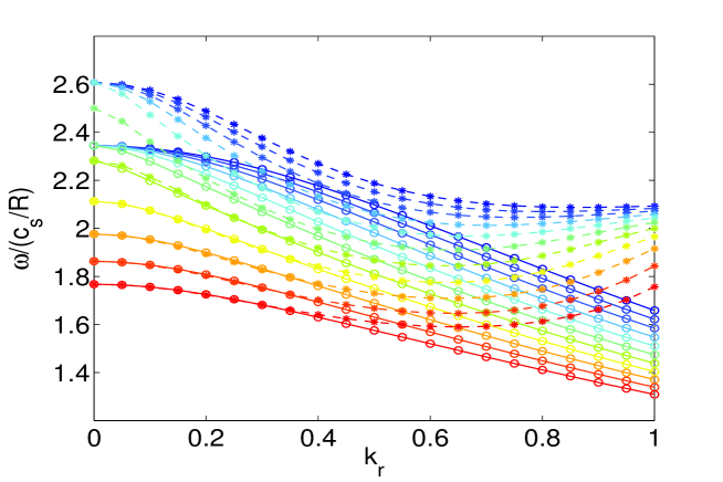
Figure 1: GAM frequencies vs $k_{r}$ with $\beta$ and $\nu$ as parameters. Color coding: blue$(\beta=0)$ to red$(\beta=0.04)$ in steps of $0.004$. Line styles: solid for $\nu=0$ and dashed for $\nu=0.1$. $\tau=1$, $q=4$.

The radial group velocity at any $\beta$ and $k_{r}$ is either zero or negative when $\nu=0$. Whereas at finite $\nu$ the radial group velocity may either be negative, zero or positive depending on the values of $\beta$, $\nu$ and $k_{r}$.

Self consistent inclusion of flux surface averaged temperature leads to the following modification of GAM dispersion in collisionless electrostatic limit

$$\omega^{2}\left(1+k_{r}^{2}\right)=R_{Tn\sin\theta}+\left(\frac{\varepsilon_{n}^{2}}{2}+\left(\frac{\varepsilon_{n}}{2q}\right)^{2}\right)\left(1+\tau_{i}+\tau_{i}R_{Tsin\theta n\sin\theta}\right)$$ (35)

where the response $R_{Tsin\theta n\sin\theta}$ of $\langle T\sin\theta\rangle$ to $\langle n\sin\theta\rangle$

$$R_{Tsin\theta n\sin\theta}=\frac{2/3}{1-\frac{1}{2}R_{TT\sin\theta}^{2}}$$

and the response $R_{Tn\sin\theta}$ of $\langle T\rangle$ to $\langle n\sin\theta\rangle$ is given by

$$R_{Tn\sin\theta}=R_{TT\sin\theta}R_{Tsin\theta n\sin\theta}$$

where $R_{TT\sin\theta}$ represents the response of $\langle T\rangle$ to $\langle T\sin\theta\rangle$

$$R_{TT\sin\theta}=-\frac{1}{\omega}\frac{5\epsilon_{n}}{3}k_{r}$$

On switching off the response $R_{TT\sin\theta}$, the equation 35 reduces to the simpler equation 34. Solutions of equation (35) are compared with the solutions of equation(34). It is seen that with self consistent treatment of the flux surface averaged ion temperature equation the frequency becomes non-monotonous in $k_{r}$; decreasing at small $k_{r}$ but increasing at large $k_{r}$. This can yield both inward and outward group velocites depending on the valaues of $k_{r}$. Moreover another lower frequency branch appears (red curve in Fig.(2)) which increases with $k_{r}$ with the vanishing frequency at $k_{r}=0$.

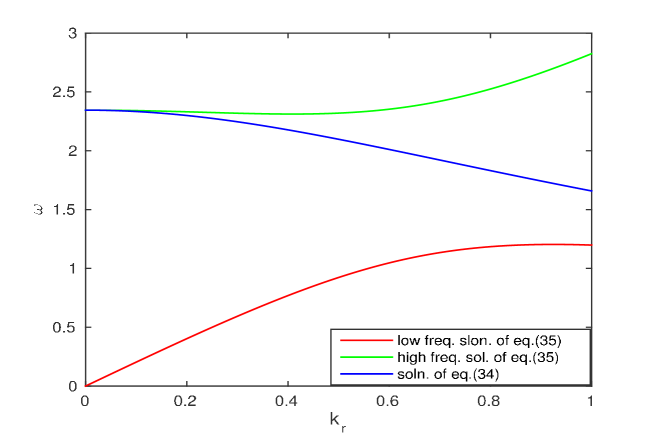
Figure 2: GAM frequencies vs $k_{r}$ with effect of $\langle T_{i}\rangle$ for $\nu=0$, $\beta=0$

Inclusion of $\langle T\rangle$ and $\langle n\rangle$ responses in the more general dispersion relation equation 33 for finite collisionality and beta is straightfoward but tedious. The most general dispersion relation in principle can be obtained from

$$|\lambda I-M|=0$$ (36)

where the imaginary part of the eigenvalue $\lambda$ gives the real frequency and the real part of $\lambda$ gives the growth rate. It can best be studied numericaly for the eigenvalues $\lambda$ of the matrix $M$. Fig.3 shows the dispersion relation with the self-consistent treatment of the average density and temperature equations. It is seen that in general the frequency decreases with $\beta$ with the rate of decrese depending on the values of $k_{r}$ and $\nu$. However for a given $\beta$ value the frequency increases with $\nu$ for $0\leq k_{r}<0.58$ and decreases with $\nu$ for $k_{r}\gtrsim 0.58$. The major differece between the exact dispersion relations Fig.3 and the approximate one in Fig.1 are the following. The collisionality may enhance or reduce GAM frequency depending on the value of $k_{r}$ in the exact case whereas collisionality has always up shifting effect on GAM frequency in the approximate model. Also in the exact model the down shifting effect of $\beta$ on GAM frequency is much less pronounced than in the approximate model.

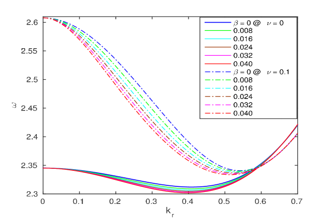
Figure 3: GAM frequencies vs $k_{r}$ with effect of $\langle T_{i}\rangle$ and $\langle n\rangle$ for $\nu=0$ and $0.1$ for different values of $\beta$

III.2 Comparison with experiment

We compare the theoretical GAM frequency as given by the dispersion relations (33), (36) and the with the experimental GAM frequency observed in the Tore Supra tokamak for two different values of collisionality (i.e. shots $\#45494$ and $\#45511$) (vermare:2011, ). Equilibrium profiles of density and temperature are shown in Fig.4. The temperature ratio $\tau_{i}$ is greater than $1$ towards the edge but less than $1$ towards the core. The density remains almost the same towards the edge in these two discharges. Radial profiles of collisionality and beta, which are calculated using these equilibrium profiles, are shown in Fig.5.

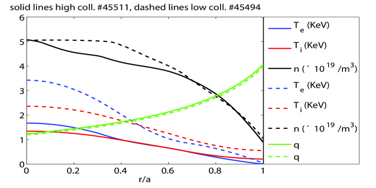
Figure 4: Equilibrium profiles at two different collisionalities. Solid lines are from high collisionality shot $\#45511$and dashed lines from low collisionality shot $\#45494$.

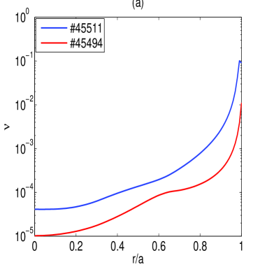
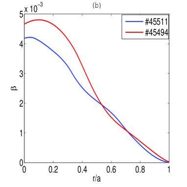
Figure 5: (a) Radial profiles of collisionalities, (b) Radial profiles of plasma beta.

The radial profiles of experimental GAM frequencies are compared against the theoretical values as obtained from equations (33), (34), (36) and from Sugama’s formula(sugama:2006, ) for $k_{r}=0$ are shown in Fig. 6. Notice that our theoretical frequency compares well with Sugama’s for both the shots but experimental frequencies are lower than both. The frequency increases inward from the edge, which is consistent with increase of temperature, but the absolute values of experimental frequencies are about $50\%$ below the theoretical values, consistently. We discuss below if this is due to finite $k_{r}$. Moreover, the experimental frequency is higher in low collisionality shots than in high collisionality shots. This might give the impression that GAM frequency goes down with collisionality, which is opposite to the theoretical prediction shown in the Fig.1? This is in fact probably due to the change in temperature profiles between the two shots, rather than the effect of collisionality.

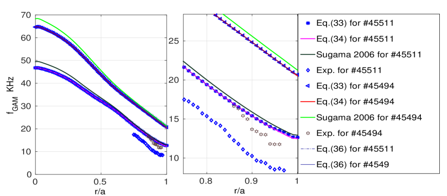
Figure 6: Comparisons between experiment and theory.

The profiles of theoretical GAM frequencies with and without collisions differs only slightly towards the edge where collisionality is higher than in the core. This shows that the collisionality and beta values are too low to make an appreciable impact on the frequency. However the absolute values of GAM frequencies are higher for low collisionality shots than for high collisionality shots, which is consistent with the upshift in temperature profiles as seen in Fig.4.

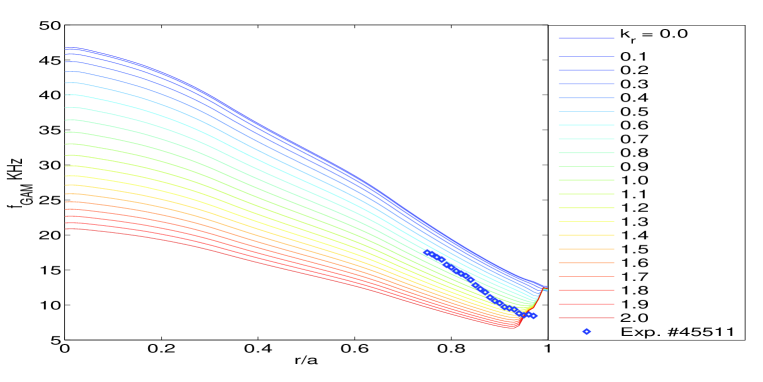
Figure 7: Radial scan of GAM frequency with $k_{r}\rho_{s}$ as parameter for high coll. shots $\#45511$

If one tries to explain the observed discrepancy between the theoretical and the experimental frequencies by invoking a finite $k_{r}$ for the GAM one notes that the GAM frequency, as predicted by Eqn 33 goes down with increasing $k_{r}$ at any radius as shown in Figs.7 and 8. However it goes up with $k_{r}$ at the edge since collisionality is felt stronger at shorter scale lengths. The frequency values computed by assuming a finite $k_{r}$ intersect with experimental observations for different wave numbers at different radii. In order to match with experimental observations, the radial wavenumber of the GAM has to increase with radius. The overlapping region of $k_{r}$ for high collisionality shots is $[0.7,1.5]$ and for low collisionality shots is $[1.3,1.7]$.

However we think that such a profile of $k_{r}$ is rather unrealistic and is probably not the explanation of the observed discrepancy. The reason being that on self-consistent inclusion of $\langle n\rangle$ and $\langle T_{i,e}\rangle$ responses through equation (36) breaks the monotonically decreasing behavior of GAM frequency on $k_{r}$. Another important reason for this conclusion is that, in fact when other harmonics of the GAMs are considered (i.e. $m=2$, $m=3$ etc.), which are linearly coupled to $m=1$, the $k_{r}$ dependence may be observed to change substantially. The gap between experiment and theory increases with $k_{r}$ at high $k_{r}$ on self-consistent inclusion of $\langle n\rangle$ and $\langle T_{i,e}\rangle$ responses at any radius as can be seen in the figures (9) and (10).

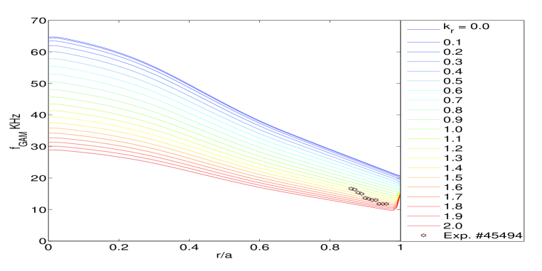
Figure 8: Radial scan of GAM frequency with $k_{r}\rho_{s}$ as parameter for low coll. shots $\#45494$

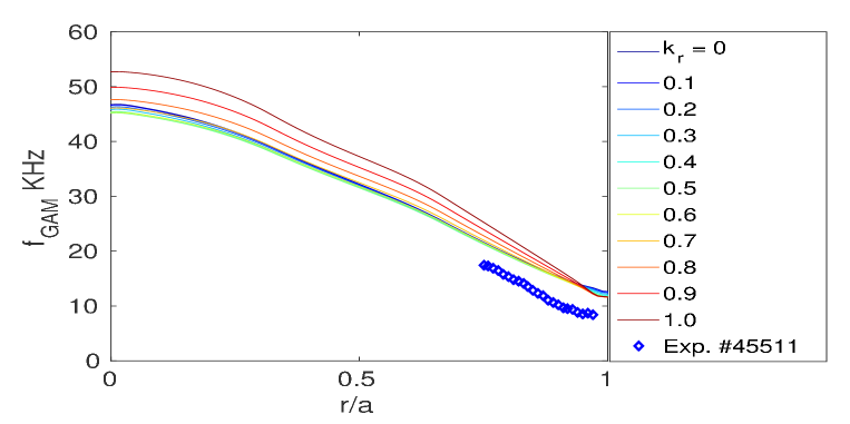
Figure 9: Radial scan of GAM frequency with $k_{r}\rho_{s}$ as parameter for high coll. shots $\#45511$, with self-consist treatment of $\langle T_{i,e}\rangle$ and $\langle n\rangle$

Figure 10: Radial scan of GAM frequency with $k_{r}\rho_{s}$ as parameter for low coll. shots $\#45494$, with self-consist treatment of $\langle T_{i,e}\rangle$ and $\langle n\rangle$

IV Conclusions

Using the reduced Braginskii equations under the drift approximation, a set of nonlinear electromagnetic equations retaining plasma beta and electron ion collisionality were obtained. Appropriate flux surface averaging were applied on the resulting set of equations in order to derive a fully nonlinear set of equations for the GAMs. This approach clearly shows that the GAM perturbations consist of $\langle\phi\rangle$, $\langle\phi\sin\theta\rangle$, $\langle n\sin\theta\rangle$, $\langle T_{i,e}\sin\theta\rangle$, $\langle v_{\parallel}\cos\theta\rangle$,$\langle A_{\parallel}\cos\theta\rangle$ up to the first poloidal harmonic. These equations can be used for studying both the nonlinear drive and the linear oscillation of the GAM in a collisional, electromagnetic model of the plasma edge. However, one needs a better closure(hammet:1990, ; Beer:1995, ; sugama:2001, ) in order to describe the collisionless GAM damping, which can in principle be included in the current model. Note however that initial studies in Tore Supra suggest that GAM damping near the edge region is mainly collisional as well.

Linearizing these equations, a general linear dispersion relation is obtained, which contains the effects of electron ion collisionality and plasma beta. Following results are obtained without $\langle n\rangle$ and $\langle T_{i,e}\rangle$. At zero collisionality and beta, the GAM frequency monotonically decreases with $k_{r}$. At finite beta the GAM frequency shifts down preserving the monotonically decreasing nature with $k_{r}$. At finite collisionality and low beta the frequency is shifted up, decreasing in $k_{r}$ at low $k_{r}$ and increasing at high $k_{r}$. The upshift in frequency with collisionality is more prominent at low and high $k_{r}$ at low beta but, at high beta the collisional upshift is seen only at high $k_{r}$ values. However with self-consistent responses of $\langle n\rangle$ and $\langle T_{i,e}\rangle$ the results are modified to the following. At zero collisionality and beta, the GAM frequency decreases with $k_{r}$ at low $k_{r}$ and incerases at high $k_{r}$. At finite beta the GAM frequency shifts down preserving the same non-monotonic decreasing nature. However the amount of down shift is more prominent in a small wave number range centered around $k_{r}\sim 0.4$. At finite collisionality the frequency is shifted up at low $k_{r}$ and shifted down at high $k_{r}$, still preserving the non-monotonic behavior of frequency decreasing in $k_{r}$ at low $k_{r}$ and increasing at high $k_{r}$. The upshift in frequency with collisionality is more at low $k_{r}$ than the down shift at high $k_{r}$. We argue that these linear trends for the GAM frequency should be retained in the nonlinear regime, since the nonlinearity acts mainly as a source term for the GAM, and does not modify its response.

The theoretical GAM frequencies obtained this way, were then compared to two TORE SUPRA shots, which were part of a collisionality scan and a consistent discrepancy were observed where the absolute values of experimental frequencies were about $50\%$ below the theoretical values for $k_{r}=0$. In fact, without the $\langle n\rangle$ and $\langle T_{i,e}\rangle$ responses the experimental GAM frequencies may be tailored to match the theoretical values by assuming finite $k_{r}$ values in the range $k_{r}\in[0.7,1.5]$ for the high collisionality shots and $k_{r}\in[1.3,1.7]$ for the low collisionality shot. However since these values are rather large, and since the $k_{r}$ dependence is mainly a feature of taking only the first poloidal harmonic of GAM, it is argued that “finite $k_{r}$ effects” probably does not explain the observed discrepancy. Also the self consistent accounting of $\langle n\rangle$ and $\langle T_{i,e}\rangle$ responses makes the experiment-theory disagreement even worst on increasing $k_{r}$.

Note also that while the experimental GAM frequencies are lower at high collisionality than at low collisionality, this observed trend is due to the change in the temperature profiles and not due to the change in collisionality and plasma beta. This implies that in order to scan the collisionality dependence of the GAM frequency, one has to keep the temperature constant. Since these shots were part of a collisionality scan for the confinement, it was the other dimensionless variables, such as $\rho_{*}$ etc. who were kept constant.

These results leave the question of the discrepancy between the GAM frequency measured in Tore Supra and the theoretical prodictions. Notice that the discrepancy is equally important if one uses a more complex gyrokinetic formula, which is shown in figure 6. We think that future work should include higher GAM harmonics in a similar fluid model of the edge, which may hopefully resolve this discrepancy.

Appendix A The matrix M

The matrix $M$ in the equation 29 is

$$M=(M_{n};M_{\phi};M_{T_{i}};M_{T_{e}};M_{n\sin\theta};M_{\phi\sin\theta};M_{A_{||}\cos\theta};M_{v_{||}\cos\theta};M_{T_{i}\sin\theta};M_{T_{e}\sin\theta})$$ (37)

where

$$M_{n}=(0,0,0,0,-i\epsilon_{n}k_{r},i\epsilon_{n}k_{r},0,0,0,i\epsilon_{n}k_{r})$$ (38)

$$M_{\phi}=(0,0,0,0,i\epsilon_{n}(1+\tau_{i})/k_{r},0,0,0,i\epsilon_{n}\tau_{i}/k_{r},i\epsilon_{n}/k_{r})$$ (39)

$$M_{T_{i}}=(0,0,0,0,-i2\epsilon_{n}k_{r}/3,i2\epsilon_{n}k_{r}/3,0,0,i5\epsilon_{n}k_{r}/3,-i2\epsilon_{n}k_{r}/3)$$ (40)

$$M_{T_{e}}=(0,0,0,0,-i2\epsilon_{n}k_{r}/3,i2\epsilon_{n}k_{r}/3,0,0,0,-i7\epsilon_{n}k_{r}/3)$$ (41)

$$M_{n\sin\theta}=(-i\epsilon_{n}k_{r}/2,i\epsilon_{n}k_{r}/2,0,-i\epsilon_{n}k_{r}/2,0,0,-\epsilon_{n}k_{r}^{2}/2q,\epsilon_{n}/2q,0,0)$$ (42)

$$M_{\phi\sin\theta}=(-i\epsilon_{n}(1+\tau_{i})/2k_{r},0,i\epsilon_{n}\tau_{i}/2k_{r},i\epsilon_{n}/2k_{r},0,0,\epsilon_{n}/2q,0,0,0)$$ (43)

$$M_{A_{||}\cos\theta}=(0,0,0,0,\epsilon_{n}/\beta q,-\epsilon_{n}/\beta q,-\nu k_{r}^{2}2/\beta,0,0,1.71\epsilon_{n}/\beta q)$$ (44)

$$M_{v_{||}\cos\theta}=(0,0,0,0,-\epsilon_{n}(1+\tau_{i})/2q,0,0,0,-\epsilon_{n}\tau_{i}/2q,-\epsilon_{n}/2q)$$ (45)

$$M_{T_{i}\sin\theta}=(-i\epsilon_{n}k_{r}/3,i\epsilon_{n}k_{r}/3,0,-i\epsilon_{n}k_{r}7/6,0,0,-\epsilon_{n}k_{r}^{2}1.38/2q,\epsilon_{n}/6q,0,-1.07(\epsilon_{n}/2q)^{2}/\nu)$$ (46)

References

- (1) P. H. Diamond, S.-I. Itoh, K. Itoh, and T. S. Hahm, Plasma Physics and Controlled Fusion 47, R35 (2005), http://stacks.iop.org/0741-3335/47/i=5/a=R01.
- (2) N. Winsor, J. L. Johnson, and J. M. Dawson, Physics of Fluids 11, 2448 (1968).
- (3) K. Miki, Y. Kishimoto, N. Miyato, and J. Q. Li, Phys. Rev. Lett. 99, 145003 (Oct 2007), http://link.aps.org/doi/10.1103/PhysRevLett.99.145003.
- (4) K. Miki, Y. Kishimoto, J. Li, and N. Miyato, Physics of Plasmas (1994-present) 15, 052309 (2008), http://scitation.aip.org/content/aip/journal/pop/15/5/10.1063/1.2908742%.
- (5) G. Y. Fu, Phys. Rev. Lett. 101, 185002 (Oct 2008), http://link.aps.org/doi/10.1103/PhysRevLett.101.185002.
- (6) G. Y. FU, Journal of Plasma Physics 77, 457 (8 2011), ISSN 1469-7807, http://journals.cambridge.org/article_S0022377810000619.
- (7) Z. Qiu, F. Zonca, and L. Chen, Plasma Physics and Controlled Fusion 52, 095003 (2010), http://stacks.iop.org/0741-3335/52/i=9/a=095003.
- (8) Z. Qiu, F. Zonca, and L. Chen, Physics of Plasmas (1994-present) 19, 082507 (2012), http://scitation.aip.org/content/aip/journal/pop/19/8/10.1063/1.4745191%.
- (9) D. Zarzoso, X. Garbet, Y. Sarazin, R. Dumont, and V. Grandgirard, Physics of Plasmas (1994-present) 19, 022102 (2012), http://scitation.aip.org/content/aip/journal/pop/19/2/10.1063/1.3680633%.
- (10) L. Wang, J. Q. Dong, Z. He, H. He, and Y. Shen, Physics of Plasmas (1994-present) 21, 072511 (2014), http://scitation.aip.org/content/aip/journal/pop/21/7/10.1063/1.4890467%.
- (11) J.-B. Girardo, D. Zarzoso, R. Dumont, X. Garbet, Y. Sarazin, and S. Sharapov, Physics of Plasmas (1994-present) 21, 092507 (2014), http://scitation.aip.org/content/aip/journal/pop/21/9/10.1063/1.4895479%.
- (12) N. Chakrabarti, R. Singh, P. K. Kaw, and P. N. Guzdar, Physics of Plasmas (1994-present) 14, 052308 (2007), http://scitation.aip.org/content/aip/journal/pop/14/5/10.1063/1.2732167%.
- (13) N. Chakrabarti, P. N. Guzdar, R. G. Kleva, V. Naulin, J. J. Rasmussen, and P. K. Kaw, Physics of Plasmas (1994-present) 15, 112310 (2008), http://scitation.aip.org/content/aip/journal/pop/15/11/10.1063/1.302831%1.
- (14) P. N. Guzdar, N. Chakrabarti, R. Singh, and P. K. Kaw, Plasma Physics and Controlled Fusion 50, 025006 (2008), http://stacks.iop.org/0741-3335/50/i=2/a=025006.
- (15) F. Zonca and L. Chen, EPL (Europhysics Letters) 83, 35001 (2008), http://stacks.iop.org/0295-5075/83/i=3/a=35001.
- (16) P. N. Guzdar, R. G. Kleva, N. Chakrabarti, V. Naulin, J. J. Rasmussen, P. K. Kaw, and R. Singh, Physics of Plasmas (1994-present) 16, 052514 (2009), http://scitation.aip.org/content/aip/journal/pop/16/5/10.1063/1.3143125%.
- (17) J. Yu and X. Gong, Nuclear Fusion 53, 123027 (2013), http://stacks.iop.org/0029-5515/53/i=12/a=123027.
- (18) L. Chen, Z. Qiu, and F. Zonca, EPL (Europhysics Letters) 107, 15003 (2014), http://stacks.iop.org/0295-5075/107/i=1/a=15003.
- (19) K. Itoh, K. Hallatschek, S.-I. Itoh, P. H. Diamond, and S. Toda, Physics of Plasmas (1994-present) 12, 062303 (2005), http://scitation.aip.org/content/aip/journal/pop/12/6/10.1063/1.1922788%.
- (20) K. Hallatschek and D. Biskamp, Phys. Rev. Lett. 86, 1223 (Feb 2001), http://link.aps.org/doi/10.1103/PhysRevLett.86.1223.
- (21) G. D. Conway, B. Scott, J. Schirmer, M. Reich, A. Kendl, and the ASDEX Upgrade Team, Plasma Phys. Control. Fusion 47, 1165 (2005).
- (22) A. Krämer-Flecken, S. Soldatov, H. R. Koslowski, and O. Zimmermann (TEXTOR Team), Phys. Rev. Lett. 97, 045006 (Jul 2006), http://link.aps.org/doi/10.1103/PhysRevLett.97.045006.
- (23) G. R. McKee, D. K. Gupta, R. J. Fonck, D. J. Schlossberg, M. W. Shafer, and P. Gohil, Plasma Phys. Control. Fusion 48, S123 (2006).
- (24) L. Vermare, P. Hennequin, Ö. D. Gürcan, and the Tore Supra Team, Nuclear Fusion 52, 063008 (2012).
- (25) C. Holland, A. E. White, G. R. McKee, M. W. Shafer, J. Candy, R. E. Waltz, L. Schmitz, and G. R. Tynan, Physics of Plasmas 16, 052301 (2009).
- (26) T. Rafiq, G. Bateman, A. H. Kritz, and A. Y. Pankin, Physics of Plasmas (1994-present) 17, 082511 (2010), http://scitation.aip.org/content/aip/journal/pop/17/8/10.1063/1.3478979%.
- (27) F. Militello and W. Fundamenski, Plasma Physics and Controlled Fusion 53, 095002 (2011), http://stacks.iop.org/0741-3335/53/i=9/a=095002.
- (28) S. I. Braginskii, Reviews of Plasma Physics edited by M. A. Leontovich I, 205 (1965).
- (29) A. Zeiler, J. F. Drake, and B. Rogers, Physics of Plasmas (1994-present) 4 (1997).
- (30) C. Nguyen, X. Garbet, and A. I. Smolyakov, Physics of Plasmas (1994-present) 15, 112502 (2008), http://scitation.aip.org/content/aip/journal/pop/15/11/10.1063/1.300804%8.
- (31) R. Singh and O. D. Gurcan, Physics of Plasmas, (to be submitted for publication)(2014).
- (32) J. Wesson, Tokamaks (Oxford Science Publications, 1997).
- (33) P. Ricci and B. N. Rogers, Phys. Rev. Lett. 104, 145001 (Apr 2010), http://link.aps.org/doi/10.1103/PhysRevLett.104.145001.
- (34) P. Beyer, X. Garbet, and P. Ghendrih, Physics of Plasmas (1994-present) 5 (1998).
- (35) V. Naulin, A. Kendl, O. E. Garcia, A. H. Nielsen, and J. J. Rasmussen, Physics of Plasmas (1994-present) 12, 052515 (2005), http://scitation.aip.org/content/aip/journal/pop/12/5/10.1063/1.1905603%.
- (36) B. D. Scott, New Journal of Physics 7, 92 (2005), http://stacks.iop.org/1367-2630/7/i=1/a=092.
- (37) B. Dudson, M. Umansky, X. Xu, P. Snyder, and H. Wilson, Computer Physics Communications 180, 1467 (2009), ISSN 0010-4655, http://www.sciencedirect.com/science/article/pii/S0010465509001040.
- (38) L. Wang and P. H. Diamond, Phys. Rev. Lett. 110, 265006 (Jun 2013), http://link.aps.org/doi/10.1103/PhysRevLett.110.265006.
- (39) G. L. Falchetto, M. Ottaviani, X. Garbet, and A. Smolyakov, Physics of Plasmas (1994-present) 14, 082304 (2007), http://scitation.aip.org/content/aip/journal/pop/14/8/10.1063/1.2755944%.
- (40) D. Zhou, Physics of Plasmas (1994-present) 14, 104502 (2007), http://scitation.aip.org/content/aip/journal/pop/14/10/10.1063/1.279374%0.
- (41) L. Wang, J. Q. Dong, Y. Shen, and H. D. He, Physics of Plasmas (1994-present) 18, 052506 (2011), http://scitation.aip.org/content/aip/journal/pop/18/5/10.1063/1.3590892%.
- (42) A. I. Smolyakov, C. Nguyen, and X. Garbet, Plasma Physics and Controlled Fusion 50, 115008 (2008), http://stacks.iop.org/0741-3335/50/i=11/a=115008.
- (43) M. F. Bashir, A. I. Smolyakov, A. G. Elfimov, A. V. Melnikov, and G. Murtaza, Physics of Plasmas (1994-present) 21, 082507 (2014), http://scitation.aip.org/content/aip/journal/pop/21/8/10.1063/1.4891883%.
- (44) H. Berk, C. Boswell, D. Borba, A. Figueiredo, T. Johnson, M. Nave, S. Pinches, S. Sharapov, and J. E. contributors, Nuclear Fusion 46, S888 (2006), http://stacks.iop.org/0029-5515/46/i=10/a=S04.
- (45) C. A. de Meijere, S. Coda, Z. Huang, L. Vermare, T. Vernay, V. Vuille, S. Brunner, J. Dominski, P. Hennequin, A. Kramer-Flecken, G. Merlo, L. Porte, and L. Villard, Plasma Physics and Controlled Fusion 56, 072001 (2014), http://stacks.iop.org/0741-3335/56/i=7/a=072001.
- (46) H. SUGAMA and T.-H. WATANABE, Journal of Plasma Physics 72, 825 (12 2006), ISSN 1469-7807, http://journals.cambridge.org/article_S0022377806004958.
- (47) Z. Gao, K. Itoh, H. Sanuki, and J. Q. Dong, Physics of Plasmas (1994-present) 13, 100702 (2006), http://scitation.aip.org/content/aip/journal/pop/13/10/10.1063/1.235972%2.
- (48) Z. Gao, K. Itoh, H. Sanuki, and J. Q. Dong, Physics of Plasmas (1994-present) 15, 072511 (2008), http://scitation.aip.org/content/aip/journal/pop/15/7/10.1063/1.2956993%.
- (49) L. Vermare, P. Hennequin, Ã. D. GÃŒrcan, C. Bourdelle, F. Clairet, X. Garbet, R. Sabot, and the Tore Supra Team, Physics of Plasmas (1994-present) 18, 012306 (2011), http://scitation.aip.org/content/aip/journal/pop/18/1/10.1063/1.3536648%.
- (50) G. W. Hammett and F. W. Perkins, Phys. Rev. Lett. 64, 3019 (Jun 1990), http://link.aps.org/doi/10.1103/PhysRevLett.64.3019.
- (51) M. A. Beer, Ph.D. thesis, Princeton University (1995).
- (52) H. Sugama, T.-H. Watanabe, and W. Horton, Physics of Plasmas (1994-present) 8 (2001).