Homotopy Continuation Approaches
for Robust SV Classification and Regression

Abstract

In support vector machine (SVM) applications with unreliable data that contains a portion of outliers, non-robustness of SVMs often causes considerable performance deterioration. Although many approaches for improving the robustness of SVMs have been studied, two major challenges remain in robust SVM learning. First, robust learning algorithms are essentially formulated as non-convex optimization problems because the loss function must be designed to alleviate the influence of outliers. It is thus important to develop a non-convex optimization method for robust SVM that can find a good local optimal solution. The second practical issue is how one can tune the hyperparameter that controls the balance between robustness and efficiency. Unfortunately, due to the non-convexity, robust SVM solutions with slightly different hyper-parameter values can be significantly different, which makes model selection highly unstable. In this paper, we address these two issues simultaneously by introducing a novel homotopy approach to non-convex robust SVM learning. Our basic idea is to introduce parametrized formulations of robust SVM which bridge the standard SVM and fully robust SVM via the parameter that represents the influence of outliers. We characterize the necessary and sufficient conditions of the local optimal solutions of robust SVM, and develop an algorithm that can trace a path of local optimal solutions when the influence of outliers is gradually decreased. An advantage of our homotopy approach is that it can be interpreted as simulated annealing, a common approach for finding a good local optimal solution in non-convex optimization problems. In addition, our homotopy method allows stable and efficient model selection based on the path of local optimal solutions. Empirical performances of the proposed approach are demonstrated through intensive numerical experiments both on robust classification and regression problems.

1 Introduction

The support vector machine (SVM) has been one of the most successful machine learning algorithms [1, 2, 3]. However, in recent practical machine learning applications with less reliable data that contains a portion of outliers (e.g., consider situations where the labels are automatically obtained by semi-supervised learning [4, 5] or manually annotated in crowdsourcing framework [6, 7]), non-robustness of the SVM often causes considerable performance deterioration. See Figure1 for examples of robust classification and regression.

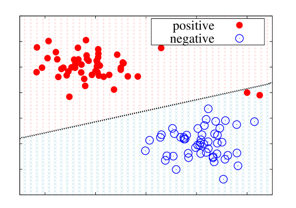
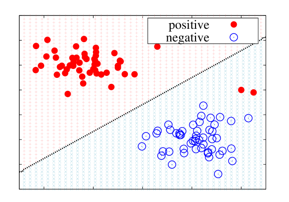
(a) Standard SVC (b) Robust SVC

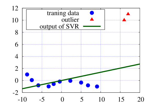
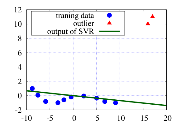
(c) Standard SVR (d) Robust SVR

Figure 1: Illustrative examples of (a) standard SVC (classification) and (b) robust SVC, (c) standard SVR (regression) and (d) robust SVR on toy dataset. In robust SVM, the classification and regression results are not sensitive to the two red outliers in the right-hand side of the plots.

1.1 Limitations of Existing Robust Classification and Regression

Although a great deal of efforts have been devoted to improving the robustness of SVM and other similar learning algorithms [8, 9, 10, 11, 12, 13, 14, 15, 16, 17, 18], the problem of learning SVM under massive noise still poses two major challenges.

First, robust learning algorithms are essentially formulated as non-convex optimization problems because the loss function must be designed to alleviate the effect of outliers (see the robust loss functions for classification and regression problems in Figure3 and Figure3). Since there could be many local optimal solutions in non-convex optimization problems, it is important to develop non-convex optimization tricks such as simulated annealing [19] that enables us to find good local optimal solution.

The second practiall issue is how to make a balance between robustness and efficiency. Any robust SVM formulations contain an additional hyper-parameter for controling the trade-off between robustness and efficiency. Since such a hyper-parameter gorverns the influence of outliers on the model, it must be carefully tuned based on the property of noise contained in the data set. In practice, we need to empirically select an appropriate value for the hyper-parameter, e.g., by cross-validation, because we usually do not have sufficient knowledge about the noise in advance. Furthermore, due to the non-convexity, robust SVM solutions with slightly different hyper-parameter values can be significantly different, which makes model selection highly unstable.

In this paper, we address these two issues simultaneously by introducing a novel homotopy approach to robust SV classification (SVC) and SV regression (SVR) learnings . Our basic idea is to consider parametrized formulations of robust SVC and SVR which bridge the standard SVM and fully robust SVM via a parameter that gorverns the influence of outliers. We use homotopy methods [20, 21, 22, 23] for tracing a path of solutions when the influence of outliers is gradually decreased. We call the parameter as the robustness parameter and the path of solutions obtained by tracing the robustness parameter as the robustification path. Figure3 and Figure3 illustrate how the robust loss functions for classification and regression problems can be gradually robustified, respectively.

1.2 Our contributions

Our first technical contribution is in analyzing the properties of the robustification path for both classification and regression problems. In particular, we derive the necessary and sufficient conditions for SVC and SVR solutions to be locally optimal (note that the well-known Karush-Khun Tucker (KKT) conditions are only necessary, but not sufficient). Interestingly, the analyses indicate that the robustification paths contain a finite number of dicontinuous points. To the best of our knowledge, the above property of robust learning has not been known previously.

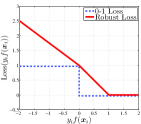
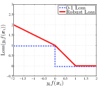
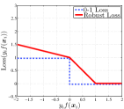
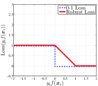
$\theta=1$, $s=0$	$\theta=0.75$, $s=0$	$\theta=0.5$, $s=0$	$\theta=0.25$, $s=0$	$\theta=0$, $s=0$
(a) Homotopy computation with decreasing $\theta$ from 1 to 0.
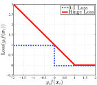
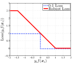
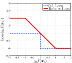
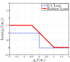
$\theta=0$, $s=-\infty$	$\theta=0$, $s=-1.5$	$\theta=0$, $s=-1$	$\theta=0$, $s=-0.5$	$\theta=0$, $s=0$
(b) Homotopy computation with decreasing $s$ from $-\infty$ to 0.

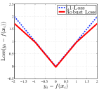
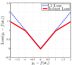
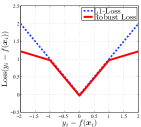
Figure 2: Robust loss functions for various homotopy parameters $\theta$ and $s$.

$\theta=1$, $s=1$	$\theta=0.75$, $s=1$	$\theta=0.5$, $s=1$	$\theta=0.25$, $s=1$	$\theta=0$, $s=1$
(a) Homotopy computation with decreasing $\theta$ from 1 to 0.
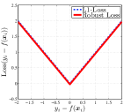
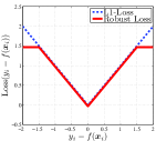
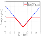
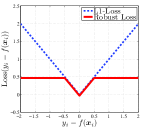
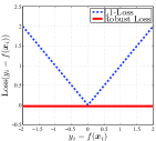
$\theta=0$, $s=\infty$	$\theta=0$, $s=1.5$	$\theta=0$, $s=1$	$\theta=0$, $s=0.5$	$\theta=0$, $s=0$
(b) Homotopy computation with decreasing $s$ from $-\infty$ to 0.

Figure 3: Regression version of robust loss functions for various homotopy parameters $\theta$ and $s$.

Our second contribution is to develop an efficient algorithm for actually computing the robustification path based on the above theoretical investigation of the geometry of robust SVM solutions. Here, we use parametric programming technique [20, 21, 22, 23], which is often used for computing the regularization path in machine learning literature. The main technical challenge here is how to handle the discontinuous points in the robustification path. We develop an algorithm that can precisely detect such discontinuous points, and jump to find a strictly better local optimal solution. Unlike solution path of convex problems [20, 21, 22, 23], our local optimal solution paths is shown to have a finite number of discrete points. We overcome this difficulty by precisely analyzing the necessary and sufficient conditions for the local optimality.

Many existing studies on robust SVM employ Concave Convex Procedure (CCCP) [24] or a variant called Difference of Convex (DC) programming [9, 10, 11, 12, 14, 15]. In these methods, a non-convex loss function is decomposed into the concave and convex parts. A local optimal solution will be obtained by iteratively solving a sequence of convex optimization problems. Local optimal solutions found by CCCP are sensitive to hyper-parameter values (for controling the robustness and efficiency balance), which makes model selection highly challenging.

Experimental results indicate that our outlier approach can find better robust SVM solutions more efficiently than alternative approaches based on CCCP. We conjecture that there are two reasons why favorable results can be obtained. At first, the robustification path shares similar advantage to simulated annealing [19]. Simulated annealing is known to find better local solutions in many non-convex optimization problems by solving a sequence of solutions along with so-called temprature parameter. If we regard the robustness parameter as the temprature parameter, our robustification path algorithm can be interpreted as simulated annealing with infinitesimal step size. Another possible explanation for favorable performances of our method is the ability of stable and efficient model selection. Since our algorithm provides the path of local solutions, unlike other non-convex optimization algorithms such as CCCP, two solutions with slightly different robustness parameter values tend to be similar, which makes model selection stable. Accoding to our experiments, choice of the robustness parameter is quite sensitive to the generalization performances. Thus, it is important to finely tune the robustness parameter. Since our algorithm can compute the path of solutions, it is much more computationally efficient than running CCCP many times at different robustness parameter values.

1.3 Structure of This Paper

After we formulate robust SVC and SVR as parametrized optimization problems in § 2, we derive in § 3 the necessary and sufficient conditions for a robust SVM solution to be locally optimal, and show that there exist a finite number of discontinuous points in the local solution path. We then propose an efficient algorithm in § 4 that can precisely detect such discontinuous points and jump to find a strictly better local optimal solution. In § 5, we experimentally demonstrate that our proposed method, named the robustification path algorithm, outperforms the existing robust SVM algorithm based on CCCP or DC programming. Finally, we conclude in § 6.

This paper is an extented version of our preliminary conference paper presented at ICML 2014 [25]. In this paper, we have extended our robusitification path framework to the regression problem, and many more experimental evaluations have been conducted. To the best of our knowledge, the homotopy method [20, 21, 22, 23] is first used in our preliminary conference paper in the context of robust learning, So far, homotopy-like methods have been (often implicitly) used for non-convex optimization problems in the context of sparse modeling [26, 27, 28] and semi-supervised learning [29].

2 Parameterized Formulation of Robust SVM

In this section, we first formulate robust SVMs for classification and regression problems, which we denote by robust SVC (SV classification) and robust SVR (SV regression), respectively. Then, we introduce parameterized formulation both for robust SVC and SVR, where the parameter gorverns the influence of outlieres to the model. The problem is reduced to ordinary non-robust SVM at one end of the parameter, while the problem corresponds to fully-robust SVM at the other end of the parameter. In the following sections, we develop algorithms for computing the path of local optimal solutions when the parameter is changed form one end to the other.

2.1 Robust SV Classification

Let us consider a binary classification problem with $n$ instances and $d$ features. We denote the training set as $\{(\mbox{\boldmath$x$}_{i},y_{i})\}_{i\in\mathbb{N}_{n}}$ where $\bm{x}_{i}\in{\cal X}$ is the input vector in the input space ${\cal X}\subset\mathbb{R}^{d}$, $y_{i}\in\{-1,1\}$ is the binary class label, and the notation $\mathbb{N}_{n}:=\{1,\ldots,n\}$ represents the set of natural numbers up to $n$. We write the decision function as

$$f(\mbox{\boldmath$x$}):=\mbox{\boldmath$w$}^{\top}\mbox{\boldmath$\phi$}(\mbox{\boldmath$x$}),$$ (1)

where $\phi$ is the feature map implicitly defined by a kernel $K$, $w$ is a vector in the feature space, and ^⊤ denotes the transpose of vectors and matrices.

We introduce the following class of optimization problems parameterized by $\theta$ and $s$:

$$\min_{\mbox{\boldmath$w$}}~{}\frac{1}{2}\|\mbox{\boldmath$w$}\|^{2}+C\sum_{i=1}^{n}\ell(y_{i}f(\mbox{\boldmath$x$}_{i});~{}\theta,s),$$ (2)

where $C>0$ is the regularization parameter which controls the balance between the first regularization term and the second loss term. The loss function $\ell$ is characterized by a pair of parameters $\theta\in[0,1]$ and $s\leq 0$ as

$$\ell(z;~{}\theta,s):=\left\{\begin{array}[]{cc}[0,1-z]_{+},&z\geq s,\\ 1-\theta z-s,&z<s,\\ \end{array}\right.$$ (5)

where $[z]_{+}:=\max\{0,z\}$. We refer to $\theta$ and $s$ as the homotopy parameters. Figure 3 shows the loss functions for several $\theta$ and $s$. The first homotopy parameter $\theta$ can be interpreted as the weight for an outlier: $\theta=1$ indicates that the influence of an outlier is the same as an inlier, while $\theta=0$ indicates that outliers are completely ignored. The second homotopy parameter $s\leq 0$ can be interpreted as the threshold for deciding outliers and inliers.

In the following sections, we consider two types of homotopy methods. In the first method, we fix $s=0$, and gradually change $\theta$ from 1 to 0 (see the top five plots in Figure 3). In the second method, we fix $\theta=0$ and gradually change $s$ from $-\infty$ to 0 (see the bottom five plots in Figure 3). Note that the loss function is reduced to the hinge loss for the standard (convex) SVC when $\theta=1$ or $s=-\infty$. Therefore, each of the above two homotopy methods can be interpreted as the process of tracing a sequence of solutions when the optimization problem is gradually modified from convex to non-convex. By doing so, we expect to find good local optimal solutions because such a process can be interpreted as simulated annealing  [19]. In addition, we can adaptively control the degree of robustness by selecting the best $\theta$ or $s$ based on some model selection scheme.

2.2 Robust SV Regression

Let us next consider a regression problem. We denote the training set of the regression problem as $\{(\bm{x}_{i},y_{i})\}_{i\in\mathbb{N}_{n}}$, where the input $\bm{x}_{i}\in{\cal X}$ is the input vector as the classification case, while the output $y_{i}\in\mathbb{R}$ is a real scalar. We consider a regression function $f(\bm{x})$ in the form of (1). SV regression is formulated as

$$\min_{\mbox{\boldmath$w$}}~{}\frac{1}{2}\|\mbox{\boldmath$w$}\|^{2}+C\sum_{i=1}^{n}\ell(y_{i}-f(\mbox{\boldmath$x$}_{i});~{}\theta,s),$$ (6)

where $C>0$ is the regularization parameter, and the loss function $\ell$ is defined as

$$\ell(z;~{}\theta,s):=\left\{\begin{array}[]{ll}|z|,&|z|<s,\\ (|z|-s)\theta+s,&|z|\geq s.\\ \end{array}\right.$$ (9)

The loss function in (9) has two parameters $\theta\in[0,1]$ and $s\in[0,\infty)$ as the classification case. Figure 3 shows the loss functions for several $\theta$ and $s$.

3 Local Optimality

In order to use the homotopy approach, we need to clarify the continuity of the local solution path. To this end, we investigate several properties of local solutions of robust SVM, and derive the necessary and sufficient conditions. Interestingly, our analysis reveals that the local solution path has a finite number of discontinuous points. The theoretical results presented here form the basis of our novel homotopy algorithm given in the next section that can properly handle the above discontinuity issue. We first discuss the local optimality of robust SVC in detail in § 3.1 and § 3.2, and then present the corresponding result of robust SVR briefly in § 3.3.

3.1 Conditionally Optimal Solutions (for Robust SVC)

The basic idea of our theoretical analysis is to reformulate the robust SVC learning problem as a combinatorial optimization problem. We consider a partition of the instances $\mathbb{N}_{n}:=\{1,\ldots,n\}$ into two disjoint sets ${\cal I}$ and ${\cal O}$. The instances in ${\cal I}$ and ${\cal O}$ are defined as ${\cal I}$nliers and ${\cal O}$utliers, respectively. Here, we restrict that the margin $y_{i}f(\bm{x}_{i})$ of an inlier should be larger than $s$, while that of an outlier should be smaller than $s$. We denote the partition as ${\cal P}:=\{{\cal I},{\cal O}\}\in 2^{\mathbb{N}_{n}}$, where $2^{\mathbb{N}_{n}}$ is the power set of $\mathbb{N}_{n}$. Given a partition ${\cal P}$, the above restrictions define the feasible region of the solution $f$ in the form of a convex polytope:

$${\rm pol}({{\cal P}};s):=\Biggl{\{}f~{}\Biggl{|}\begin{array}[]{ll}y_{i}f(\mbox{\boldmath$x$}_{i})\geq s,&i\in{\cal I}\\ y_{i}f(\mbox{\boldmath$x$}_{i})\leq s,&i\in{\cal O}\end{array}\Biggr{\}}.$$ (12)

Using the notion of the convex polytopes, the optimization problem (2) can be rewritten as

$$\min_{{{\cal P}}\in 2^{\mathbb{N}_{n}}}\Biggl{(}\min_{f\in{\rm pol}({{\cal P}};s)}J_{{{\cal P}}}(f;\theta)\Biggr{)},$$ (13)

where the objective function $J_{{{\cal P}}}$ is defined as

$$J_{{{\cal P}}}(f;\theta):=\frac{1}{2}||\mbox{\boldmath$w$}||_{2}^{2}+C\left(\sum_{i\in{\cal I}}[1-y_{i}f(\mbox{\boldmath$x$}_{i})]_{+}+\theta\sum_{i\in{\cal O}}[1-y_{i}f(\mbox{\boldmath$x$}_{i})]_{+}\right).$$

When the partition ${{\cal P}}$ is fixed, it is easy to confirm that the inner minimization problem of (13) is a convex problem.

Definition 1 (Conditionally optimal solutions)

Given a partition ${{\cal P}}$, the solution of the following convex problem is said to be the conditionally optimal solution:

$$f^{*}_{{{\cal P}}}:=\mathop{\rm argmin}\limits_{f\in{\rm pol}({{\cal P}};s)}J_{{{\cal P}}}(f;\theta).$$ (14)

The formulation in (13) is interpreted as a combinatorial optimization problem of finding the best solution from all the $2^{n}$ conditionally optimal solutions $f^{*}_{{{\cal P}}}$ corresponding to all possible $2^{n}$ partitions.

Using the representer theorem or convex optimization theory, we can show that any conditionally optimal solution can be written as

$$f^{*}_{{{\cal P}}}(\bm{x}):=\sum_{j\in\mathbb{N}_{n}}\alpha^{*}_{j}y_{j}K(\bm{x},\bm{x}_{j}),$$ (15)

where $\{\alpha^{*}_{j}\}_{j\in\mathbb{N}_{n}}$ are the optimal Lagrange multipliers. The following lemma summarizes the KKT optimality conditions of the conditionally optimal solution $f^{*}_{{\cal P}}$.

Lemma 2

The KKT conditions of the convex problem (14) is written as

$$y_{i}f^{*}_{{{\cal P}}}(\mbox{\boldmath$x$}_{i})>1~{} \Rightarrow~{}\alpha_{i}^{*}=0,$$ (16a)

$$y_{i}f^{*}_{{{\cal P}}}(\mbox{\boldmath$x$}_{i})=1~{} \Rightarrow~{}\alpha_{i}^{*}\in[0,C],$$ (16b)

$$s<y_{i}f^{*}_{{{\cal P}}}(\mbox{\boldmath$x$}_{i})<1~{} \Rightarrow~{}\alpha_{i}^{*}=C,$$ (16c)

$$y_{i}f^{*}_{{{\cal P}}}(\mbox{\boldmath$x$}_{i})=s,i\in{\cal I}~{} \Rightarrow~{}\alpha_{i}^{*}\geq C,$$ (16d)

$$y_{i}f^{*}_{{{\cal P}}}(\mbox{\boldmath$x$}_{i})=s,i\in{\cal O}~{} \Rightarrow~{}\alpha_{i}^{*}\leq C\theta,$$ (16e)

$$y_{i}f^{*}_{{{\cal P}}}(\mbox{\boldmath$x$}_{i})<s~{} \Rightarrow~{}\alpha_{i}^{*}=C\theta.$$ (16f)

The proof is omitted because it can be easily derived based on standard convex optimization theory [30].

3.2 The necessary and sufficient conditions for local optimality (for Robust SVC)

From the definition of conditionally optimal solutions, it is clear that a local optimal solution must be conditionally optimal within the convex polytope ${\rm pol}({{\cal P}};s)$. However, the conditional optimality does not necessarily indicate the local optimality as the following theorem suggests.

Theorem 3

For any $\theta\in[0,1)$ and $s\leq 0$, consider the situation where a conditionally optimal solution $f^{*}_{{{\cal P}}}$ is at the boundary of the convex polytope ${\rm pol}({{\cal P}};s)$, i.e., there exists at least an instance such that $y_{i}f^{*}_{{{\cal P}}}(\bm{x}_{i})=s$. In this situation, if we define a new partition $\tilde{{\cal P}}:=\{\tilde{{\cal I}},\tilde{{\cal O}}\}$ as

$$\tilde{{\cal I}}\!\leftarrow\!{\cal I}\!\setminus\!\{i\in{\cal I}|y_{i}f^{*}(\mbox{\boldmath$x$}_{i})\!=\!s\}\!\cup\!\{i\in{\cal O}|y_{i}f^{*}(\mbox{\boldmath$x$}_{i})\!=\!s\},$$ (17a)

$$\tilde{{\cal O}}\!\leftarrow\!{\cal O}\!\setminus\!\{i\in{\cal O}|y_{i}f^{*}(\mbox{\boldmath$x$}_{i})\!=\!s\}\!\cup\!\{i\in{\cal I}|y_{i}f^{*}(\mbox{\boldmath$x$}_{i})\!=\!s\},$$ (17b)

then the new conditionally optimal solution $f^{*}_{\tilde{{\cal P}}}$ is strictly better than the original conditionally optimal solution $f^{*}_{{\cal P}}$, i.e.,

$$J_{\tilde{{\cal P}}}(f^{*}_{\tilde{{\cal P}}};\theta)<J_{{\cal P}}(f^{*}_{{\cal P}};\theta).$$ (18)

The proof is presented in Appendix A. Theorem 3 indicates that if $f^{*}_{{{\cal P}}}$ is at the boundary of the convex polytope ${\rm pol}({{\cal P}};s)$, i.e., if there is one or more instances such that $y_{i}f^{*}_{{\cal P}}(\bm{x}_{i})=s$, then $f^{*}_{{{\cal P}}}$ is NOT locally optimal because there is a strictly better solution in the opposite side of the boundary.

The following theorem summarizes the necessary and sufficient conditions for local optimality. Note that, in non-convex optimization problems, the KKT conditions are necessary but not sufficient in general.

Theorem 4

For $\theta\in[0,1)$ and $s\leq 0$,

$$y_{i}f^{*}(\mbox{\boldmath$x$}_{i})>1 \;\Rightarrow\; \alpha_{i}^{*}=0,$$ (19a)

$$y_{i}f^{*}(\mbox{\boldmath$x$}_{i})=1 \;\Rightarrow\; \alpha_{i}^{*}\in[0,C],$$ (19b)

$$s<y_{i}f^{*}(\mbox{\boldmath$x$}_{i})<1 \;\Rightarrow\; \alpha_{i}^{*}=C,$$ (19c)

$$y_{i}f^{*}(\mbox{\boldmath$x$}_{i})<s \;\Rightarrow\; \alpha_{i}^{*}=C\theta,$$ (19d)

$$y_{i}f^{*}(\mbox{\boldmath$x$}_{i})\neq s, \!\!\!\!\!\!\!\!\!\!\!\!\!\!\!\forall i\in\mathbb{N}_{n},$$ (19e)

are necessary and sufficient for $f^{*}$ to be locally optimal.

The proof is presented in Appendix B. The condition (19e) indicates that the solution at the boundary of the convex polytope is not locally optimal. Figure 4 illustrates when a conditionally optimal solution can be locally optimal with a certain $\theta$ or $s$.

Theorem 4 suggests that, whenever the local solution path computed by the homotopy approach encounters a boundary of the current convex polytope at a certain $\theta$ or $s$, the solution is not anymore locally optimal. In such cases, we need to somehow find a new local optimal solution at that $\theta$ or $s$, and restart the local solution path from the new one. In other words, the local solution path has discontinuity at that $\theta$ or $s$. Fortunately, Theorem 3 tells us how to handle such a situation. If the local solution path arrives at the boundary, it can jump to the new conditionally optimal solution $f^{*}_{\tilde{{\cal P}}}$ which is located on the opposite side of the boundary. This jump operation is justified because the new solution is shown to be strictly better than the previous one. Figure 4 (c) and (d) illustrate such a situation.

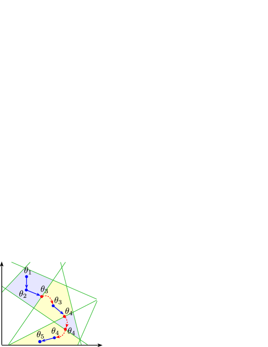
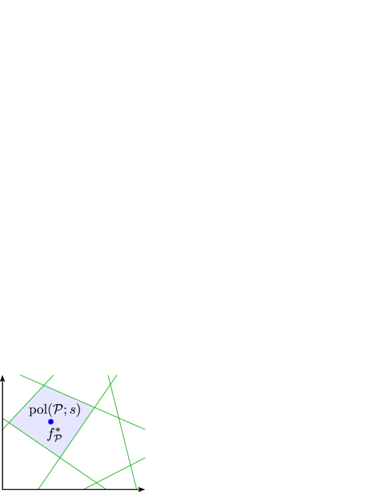
(a) Local solution path (b) Local optimum

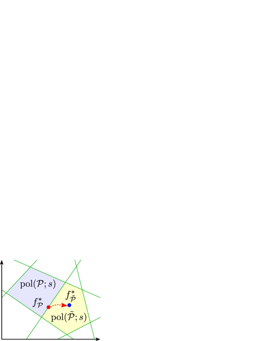
(c) Not local optimum (d) Local optimum

Figure 4: Solution space of robust SVC. (a) The arrows indicate a local solution path when $\theta$ is gradually moved from $\theta_{1}$ to $\theta_{5}$ (see § 4 for more details). (b) $f^{*}_{\cal P}$ is locally optimal if it is at the strict interior of the convex polytope ${\rm pol}({{\cal P}};s)$. (c) If $f^{*}_{\cal P}$ exists at the boundary, then $f^{*}_{\cal P}$ is feasible, but not locally optimal. A new convex polytope ${\rm pol}({\tilde{{\cal P}}};s)$ defined in the opposite side of the boundary is shown in yellow. (d) A strictly better solution exists in ${\rm pol}({\tilde{{\cal P}}};s)$.

3.3 Local optimality of SV Regression

In order to derive the necessary and sufficent conditions of the local optimality in robust SVR, with abuse of notation, let us consider a partition of the instances $\mathbb{N}_{n}$ into two disjoint sets $\mathcal{I}$ and $\mathcal{O}$, which represent inliers and outliers, respectively. In regression problems, an instance $(\bm{x}_{i},y_{i})$ is regarded as an outlier if the aboslute residual $|y_{i}-f(\bm{x}_{i})|$ is sufficiently large. Thus, we define inliers and outliers of regression problem as

$$\mathcal{I} := \{i\in\mathbb{N}_{n}|~{}|y_{i}-f(\mbox{\boldmath$x$}_{i})|<s\},$$

$$\mathcal{O} := \{i\in\mathbb{N}_{n}|~{}|y_{i}-f(\mbox{\boldmath$x$}_{i})|>s\}.$$

Given a partition ${\cal P}:=\{{\cal I},{\cal O}\}\in 2^{\mathbb{N}_{n}}$, the feasible region of the solution $f$ is represented as a convex polytope:

$${\rm pol}({\cal P};s):=\Biggl{\{}f~{}\Biggl{|}\begin{array}[]{ll}|y_{i}-f(\mbox{\boldmath$x$}_{i})|\leq s,&i\in\mathcal{I},\\ |y_{i}-f(\mbox{\boldmath$x$}_{i})|\geq s,&i\in\mathcal{O}\end{array}\Biggr{\}}.$$ (22)

Then, as in the classification case, the optimization problem (6) can be rewritten as

$$\min_{{\cal P}}\Biggl{(}\min_{f\in{\rm pol}({{\cal P}};s)}J_{{{\cal P}}}(f;\theta)\Biggr{)},$$ (23)

where the objective function $J_{{\cal P}}$ is defined as

$$J_{{\cal P}}(f;\theta)=\frac{1}{2}||\mbox{\boldmath$w$}||_{2}^{2}+C\left(\sum_{i\in\mathcal{I}}|y_{i}-f(\mbox{\boldmath$x$}_{i})|+\theta\sum_{i\in\mathcal{O}}|y_{i}-f(\mbox{\boldmath$x$}_{i})|\right).$$

Since the inner problem of (23) is a convex problem, any conditionally optimal solution can be written as

$$f^{*}_{{{\cal P}}}(\bm{x}):=\sum_{j\in\mathbb{N}_{n}}\alpha^{*}_{j}K(\bm{x},\bm{x}_{j}).$$ (24)

The KKT conditions of $f^{*}_{{{\cal P}}}(\bm{x})$ are written as

$$|y_{i}-f^{*}_{{{\cal P}}}(\mbox{\boldmath$x$}_{i})|=0~{} \Rightarrow~{}0\leq|\alpha_{i}^{*}|\leq C,$$ (25a)

$$0\leq|y_{i}-f^{*}_{{{\cal P}}}(\mbox{\boldmath$x$}_{i})|<s~{} \Rightarrow~{}|\alpha_{i}^{*}|=C,$$ (25b)

$$|y_{i}-f^{*}_{{{\cal P}}}(\mbox{\boldmath$x$}_{i})|=s,i\in\mathcal{I}~{} \Rightarrow~{}|\alpha_{i}^{*}|\geq C,$$ (25c)

$$|y_{i}-f^{*}_{{{\cal P}}}(\mbox{\boldmath$x$}_{i})|=s,i\in\mathcal{O}~{} \Rightarrow~{}|\alpha_{i}^{*}|\leq\theta C,$$ (25d)

$$|y_{i}-f^{*}_{{{\cal P}}}(\mbox{\boldmath$x$}_{i})|>s~{} \Rightarrow~{}|\alpha_{i}^{*}|=\theta C.$$ (25e)

Based on the same discussion as §3.2, the necessary and sufficient conditions for the local optimality of robust SVR are summarized as the following theorem:

Theorem 5

For $$\theta\in[0,1) s\geq 0$$ and ,

$$|y_{i}-f^{*}_{{{\cal P}}}(\mbox{\boldmath$x$}_{i})|=0~{} \Rightarrow~{}0\leq|\alpha_{i}^{*}|\leq C,$$ (26a)

$$0\leq|y_{i}-f^{*}_{{{\cal P}}}(\mbox{\boldmath$x$}_{i})|<s~{} \Rightarrow~{}|\alpha_{i}^{*}|=C,$$ (26b)

$$|y_{i}-f^{*}_{{{\cal P}}}(\mbox{\boldmath$x$}_{i})|>s~{} \Rightarrow~{}|\alpha_{i}^{*}|=\theta C,$$ (26c)

$$|y_{i}-f^{*}_{{{\cal P}}}(\mbox{\boldmath$x$}_{i})|\neq s.$$ (26d)

are necessary and sufficient for $$f^{*}$$ to be locally optimal.

We omit the proof of this theorem because they can be easily derived in the same way as Theorem 4.

4 Outlier Path Algorithm

Based on the analysis presented in the previous section, we develop a novel homotopy algorithm for robust SVM. We call the proposed method the outlier-path (OP) algorithm. For simplicity, we consider homotopy path computation involving either $\theta$ or $s$, and denote the former as OP-$\theta$ and the latter as OP-$s$. OP-$\theta$ computes the local solution path when $\theta$ is gradually decreased from 1 to 0 with fixed $s=0$, while OP-$s$ computes the local solution path when $s$ is gradually increased from $-\infty$ to 0 with fixed $\theta=0$.

The local optimality of robust SVM in the previous section shows that the path of local optimal solutions has finite discontinuous points that satisfy (19e) or (26d). Below, we introduce an algorithm that appropriately handles those discontinuous points. In this section, we only describe the algorithm for robust SVC. All the methodologies described in this section can be easily extended to robust SVR counterpart.

4.1 Overview

Algorithm 1 Outlier Path Algorithm

1:  Initialize the solution $f$ by solving the standard SVM.

2:  Initialize the partition ${\cal P}:=\{{\cal I},{\cal O}\}$ as follows:

$${\cal I}~{} \leftarrow~{}\{i\in\mathbb{N}_{n}|y_{i}f(\bm{x}_{i})\leq s\},$$

$${\cal O}~{} \leftarrow~{}\{i\in\mathbb{N}_{n}|y_{i}f(\bm{x}_{i})>s\}.$$

3:  $\theta\leftarrow 1$ for OP-$\theta$; $s\leftarrow\min_{i\in\mathbb{N}_{n}}y_{i}f(\bm{x}_{i})$ for OP-$s$.

4:  while $\theta>0$ for OP-$\theta$; $s<0$ for OP-$s$ do

5:     if ($y_{i}f(\bm{x}_{i})\neq s~{}\forall~{}i\in\mathbb{N}_{n}$) then

6:        Run C-step.

7:     else

8:        Run D-step.

9:     end if

10:  end while

The main flow of the OP algorithm is described in Algorithm 1. The solution $f$ is initialized by solving the standard (convex) SVM, and the partition ${\cal P}:=\{{\cal I},{\cal O}\}$ is defined to satisfy the constraints in (12). The algorithm mainly switches over the two steps called the continuous step (C-step) and the discontinuous step (D-step).

In the C-step (Algorithm 2), a continuous path of local solutions is computed for a sequence of gradually decreasing $\theta$ (or increasing $s$) within the convex polytope ${\rm pol}({\cal P};s)$ defined by the current partition ${\cal P}$. If the local solution path encounters a boundary of the convex polytope, i.e., if there exists at least an instance such that $y_{i}f(\bm{x}_{i})=s$, then the algorithm stops updating $\theta$ (or $s$) and enters the D-step.

In the D-step (Algorithm 3), a better local solution is obtained for fixed $\theta$ (or $s$) by solving a convex problem defined over another convex polytope in the opposite side of the boundary (see Figure 4(d)). If the new solution is again at a boundary of the new polytope, the algorithm repeatedly calls the D-step until it finds the solution in the strict interior of the current polytope.

The C-step can be implemented by any homotopy algorithms for solving a sequence of quadratic problems (QP). In OP-$\theta$, the local solution path can be exactly computed because the path within a convex polytope can be represented as piecewise-linear functions of the homotopy parameter $\theta$. In OP-$s$, the C-step is trivial because the optimal solution is shown to be constant within a convex polytope. In § 4.2 and § 4.3, we will describe the details of our implementation of the C-step for OP-$\theta$ and OP-$s$, respectively.

In the D-step, we only need to solve a single quadratic problem (QP). Any QP solver can be used in this step. We note that the warm-start approach [31] is quite helpful in the D-step because the difference between two conditionally optimal solutions in adjacent two convex polytopes is typically very small. In § 4.4, we describe the details of our implementation of the D-step. Figure 5 illustrates an example of the local solution path obtained by OP-$\theta$.

Algorithm 2 Continuous Step (C-step)

1:  while ($y_{i}f(\bm{x}_{i})\neq s~{}\forall~{}i\in\mathbb{N}_{n}$) do

2:     Solve the sequence of convex problems,

$$\min_{f\in{\rm pol}({\cal P};s)}J_{{\cal P}}(f;\theta),$$

for gradually decreasing $\theta$ in OP-$\theta$ or gradually increasing $s$ in OP-$s$.

3:  end while

Algorithm 3 Discontinuous Step (D-step)

1:  Update the partition ${\cal P}:=\{{\cal I},{\cal O}\}$ as follows:

$${\cal I}\;\leftarrow{\cal I} \setminus\{i\in{\cal I}|y_{i}f(\mbox{\boldmath$x$}_{i})=s\}\cup\{i\in{\cal O}|y_{i}f(\mbox{\boldmath$x$}_{i})=s\},$$

$${\cal O}\leftarrow{\cal O} \setminus\{i\in{\cal O}|y_{i}f(\mbox{\boldmath$x$}_{i})=s\}\cup\{i\in{\cal I}|y_{i}f(\mbox{\boldmath$x$}_{i})=s\}.$$

2:  Solve the following convex problem for fixed $\theta$ and $s$:

$$\min_{f\in{\rm pol}({\cal P};s)}J_{{\cal P}}(f;\theta).$$

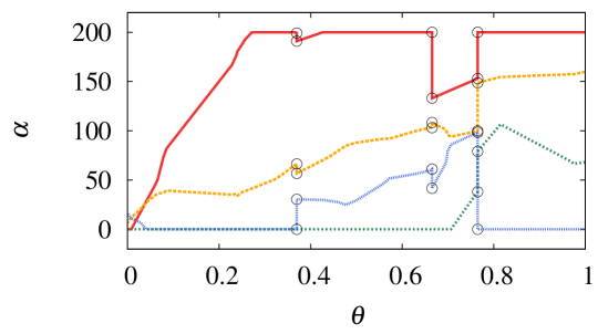
Figure 5: An example of the local solution path by OP-$\theta$ on a simple toy data set (with $C=200$). The paths of five Lagrange multipliers $\alpha^{*}_{1},\cdots,\alpha^{*}_{4}$ are plotted in the range of $\theta\in[0,1]$. Open circles represent the discontinuous points in the path. In this simple example, we had experienced three discontinuous points at $\theta=0.37,0.67$ and $0.77$.

4.2 Continuous-Step for OP-$\theta$

In the C-step, the partition ${\cal P}:=\{{\cal I},{\cal O}\}$ is fixed, and our task is to solve a sequence of convex quadratic problems (QPs) parameterized by $\theta$ within the convex polytope ${\rm pol}({\cal P};s)$. It has been known in optimization literature that a certain class of parametric convex QP can be exactly solved by exploiting the piecewise linearity of the solution path [23]. We can easily show that the local solution path of OP-$\theta$ within a convex polytope is also represented as a piecewise-linear function of $\theta$. The algorithm presented here is similar to the regularization path algorithm for SVM given in [32].

Let us consider a partition of the inliers in ${\cal I}$ into the following three disjoint sets:

$$\mathcal{R} := \{i|1<y_{i}f(\mbox{\boldmath$x$}_{i})\},$$

$$\mathcal{E} := \{i|y_{i}f(\mbox{\boldmath$x$}_{i})=1\},$$

$$\mathcal{L} := \{i|s<y_{i}f(\mbox{\boldmath$x$}_{i})<1\}.$$

For a given fixed partition $\{{\cal R},{\cal E},{\cal L},{\cal O}\}$, the KKT conditions of the convex problem (14) indicate that

$$\alpha_{i}=0~{}\forall~{}i\in{\cal R},~{}~{}\alpha_{i}=C~{}\forall~{}i\in{\cal L},~{}~{}\alpha_{i}=C\theta~{}\forall~{}i\in{\cal O}.$$

The KKT conditions also imply that the remaining Lagrange multipliers $\{\alpha_{i}\}_{i\in{\cal E}}$ must satisfy the following linear system of equations:

$$~{}~{}y_{i}f(\bm{x}_{i})=\sum_{j\in\mathbb{N}_{n}}\alpha_{j}y_{i}y_{j}K(\bm{x}_{i},\bm{x}_{j})=1~{}\forall~{}i\in{\cal E}$$

$$\Leftrightarrow~{}~{}\bm{Q}_{{\cal E}{\cal E}}\bm{\alpha}_{{\cal E}}=\mathbf{1}-\bm{Q}_{{\cal E}{\cal L}}\mathbf{1}C-\bm{Q}_{{\cal E}{\cal O}}\mathbf{1}C\theta,$$ (27)

where $\bm{Q}\in\mathbb{R}^{n\times n}$ is an $n\times n$ matrix whose $(i,j)^{\rm th}$ entry is defined as $Q_{ij}:=y_{i}y_{j}K(\mbox{\boldmath$x$}_{i},\mbox{\boldmath$x$}_{j})$. Here, a notation such as $\bm{Q}_{{\cal E}{\cal L}}$ represents a submatrix of $\bm{Q}$ having only the rows in the index set ${\cal E}$ and the columns in the index set ${\cal L}$. By solving the linear system of equations (27), the Lagrange multipliers $\alpha_{i},i\in\mathbb{N}_{n}$, can be written as an affine function of $\theta$.

Noting that $y_{i}f(\bm{x}_{i})=\sum_{j\in\mathbb{N}_{n}}\alpha_{j}y_{i}y_{j}K(\bm{x}_{i},\bm{x}_{j})$ is also represented as an affine function of $\theta$, any changes of the partition $\{{\cal R},{\cal E},{\cal L}\}$ can be exactly identified when the homotopy parameter $\theta$ is continuously decreased. Since the solution path linearly changes for each partition of $\{{\cal R},{\cal E},{\cal L}\}$, the entire path is represented as a continuous piecewise-linear function of the homotopy parameter $\theta$. We denote the points in $\theta\in[0,1)$ at which members of the sets $\{{\cal R},{\cal E},{\cal L}\}$ change as break-points $\theta_{BP}$.

Using the piecewise-linearity of $y_{i}f(\bm{x}_{i})$, we can also identify when we should switch to the D-step. Once we detect an instance satisfying $y_{i}f(\bm{x}_{i})=s$, we exit the C-step and enter the D-step.

4.3 Continuous-Step for OP-$s$

Since $\theta$ is fixed to 0 in OP-$s$, the KKT conditions (16) yields

$$\alpha_{i}=0~{}\forall~{}i\in{\cal O}.$$

This means that outliers have no influence on the solution and thus the conditionally optimal solution $f^{*}_{{\cal P}}$ does not change with $s$ as long as the partition ${\cal P}$ is unchanged. The only task in the C-step for OP-$s$ is therefore to find the next $s$ that changes the partition ${\cal P}$. Such $s$ can be simply found as

$$s~{}\leftarrow~{}\min_{i\in{\cal L}}y_{i}f(\bm{x}_{i}).$$

4.4 Discontinuous-Step (for both OP-$\theta$ and OP-$s$)

As mentioned before, any convex QP solver can be used for the D-step. When the algorithm enters the D-step, we have the conditionally optimal solution $f^{*}_{\cal P}$ for the partition ${\cal P}:=\{{\cal I},{\cal O}\}$. Our task here is to find another conditionally optimal solution $f^{*}_{\tilde{{\cal P}}}$ for $\tilde{{\cal P}}:=\{\tilde{{\cal I}},\tilde{{\cal O}}\}$ given by (17).

Given that the difference between the two solutions $f^{*}_{\cal P}$ and $f^{*}_{\tilde{{\cal P}}}$ is typically small, the D-step can be efficiently implemented by a technique used in the context of incremental learning [33].

Let us define

$$\Delta_{{\cal I}\to{\cal O}} :=\{i\in{\cal I}~{}|~{}y_{i}f_{{\cal P}}(\bm{x}_{i})=s\},$$

$$\Delta_{{\cal O}\to{\cal I}} :=\{i\in{\cal O}~{}|~{}y_{i}f_{{\cal P}}(\bm{x}_{i})=s\}.$$

Then, we consider the following parameterized problem with parameter $\mu\in[0,1]$:

$$f_{\tilde{{\cal P}}}(\bm{x}_{i};\mu):=f_{\tilde{{\cal P}}}(\bm{x}_{i})+\mu\Delta f_{i}~{}\forall~{}i\in\mathbb{N}_{n},$$

where

$$\Delta f_{i}:=y_{i}\left[\begin{array}[]{cc}\bm{K}_{i,\Delta_{{\cal I}\to{\cal O}}}&\bm{K}_{i,\Delta_{{\cal O}\to{\cal I}}}\\ \end{array}\right]\left[\begin{array}[]{c}\bm{\alpha}^{\rm(bef)}_{\Delta_{{\cal I}\to{\cal O}}}-\mathbf{1}C\theta\\ \bm{\alpha}^{\rm(bef)}_{\Delta_{{\cal O}\to{\cal I}}}-\mathbf{1}C\end{array}\right],$$

and $\bm{\alpha}^{(\rm bef)}$ be the corresponding $\bm{\alpha}$ at the beginning of the D-Step. We can show that $f_{\tilde{{\cal P}}}(\bm{x}_{i};\mu)$ is reduced to $f_{{\cal P}}(\bm{x}_{i})$ when $\mu=1$, while it is reduced to $f_{\tilde{{\cal P}}}(\bm{x}_{i})$ when $\mu=0$ for all $i\in\mathbb{N}_{n}$. By using a similar technique to incremental learning [33], we can efficiently compute the path of solutions when $\mu$ is continuously changed from 1 to 0. This algorithm behaves similarly to the C-step in OP-$\theta$. The implementation detail of the D-step is described in Appendix C.

5 Numerical Experiments

In this section, we compare the proposed outlier-path (OP) algorithm with conventional concave-convex procedure (CCCP) [24] because, in most of the existing robust SVM studies, non-convex optimization for robust SVM training are solved by CCCP or a variant called difference of convex (DC) programming [9, 10, 11, 12, 14, 15].

5.1 Setup

We used several benchmark data sets listed in Tables 2 and 2. We randomly divided data set into training (40%), validation (30%), and test (30%) sets for the purposes of optimization, model selection (including the selection of $\theta$ or $s$), and performance evaluation, respectively. For robust SVC, we randomly flipped 15% of the labels in the training and the validation data sets. For robust SVR, we first preprocess the input and output variables; each input variable was normalized so that the minimum and the maximum values are $-1$ and $+1$, respectively, while the output variable was standardized to have mean zero and variance one. Then, for the 5% of the training and the validation instances, we added an uniform noise $U(-2,2)$ to input variable, and a Gaussian noise $N(0,10^{2})$ to output variable, where $U(a,b)$ denotes the uniform distribution between $a$ and $b$ and $N(\mu,\sigma^{2})$ denotes the normal distribution with mean $\mu$ and variance $\sigma^{2}$.

Table 1: Benchmark data sets for robust SVC experiments

	Data	$n$	$d$
D1	BreastCancerDiagnostic	569	30
D2	AustralianCredit	690	14
D3	GermanNumer	1000	24
D4	SVMGuide1	3089	4
D5	spambase	4601	57
D6	musk	6598	166
D7	gisette	6000	5000
D8	w5a	9888	300
D9	a6a	11220	122
D10	a7a	16100	122
$n=\#$ of instances, $d=$ input dimension

Table 2: Benchmark data sets for robust SVR experiments

	Data	$n$	$d$
D1	bodyfat	252	14
D2	yacht_hydrodynamics	308	6
D3	mpg	392	7
D4	housing	506	13
D5	mg	1385	6
D6	winequality-red	1599	11
D7	winequality-white	4898	11
D8	space_ga	3107	6
D9	abalone	4177	8
D10	cpusmall	8192	12
D11	cadata	20640	8
$n=\#$ of instances, $d=$ input dimension

5.2 Generalization Performance

First, we compared the generalization performance. We used the linear kernel and the radial basis function (RBF) kernel defined as $K(\mbox{\boldmath$x$}_{i},\mbox{\boldmath$x$}_{j})=\exp\left(-\gamma\|\mbox{\boldmath$x$}_{i}-\mbox{\boldmath$x$}_{j}\|^{2}\right)$, where $\gamma$ is a kernel parameter fixed to $\gamma=1/d$ with $d$ being the input dimensionality. Model selection was carried out by finding the best hyper-parameter combination that minimizes the validation error. We have a pair of hyper-parameters in each setup. In all the setups, the regularization parameter $C$ was chosen from $\{0.01,0.1,1,10,100\}$, while the candidates of the homotopy parameters were chosen as follows:

• In OP-$\theta$, the set of break-points $\theta_{BP}\in[0,1]$ was considered as the candidates (note that the local solutions at each break-point have been already computed in the homotopy computation).

• In OP-$s$, the set of break-points in $[s_{C},0]$ was used as the candidates for robust SVC, where

  $$s_{C}:=\min_{i\in\mathbb{N}_{n}}y_{i}f_{\rm SVC}(\mbox{\boldmath$x$}_{i})$$

  with $f_{\rm SVC}$ being the ordinary non-robust SVC. For robust SVR, the set of break-points in $[s_{R},0.2S_{R}]$ was used as the candidates, where

  $$s_{R}:=\max_{i\in\mathbb{N}_{n}}|y_{i}-f_{\rm SVR}(\mbox{\boldmath$x$}_{i})|$$

  with $f_{\rm SVC}$ being the ordinary non-robust SVR.

• In CCCP-$\theta$, the homotopy parameter $\theta$ was selected from

  $$\theta\in\{1,0.75,0.5,0.25,0\}.$$

• In CCCP-$s$, the homotopy parameter $s$ was selected from

  $$s\in\{s_{C},0.75s_{C},0.5s_{C},0.25s_{C},0\}$$

  for robust SVC, while it was selected from

  $$s\in\{s_{R},0.8s_{R},0.6s_{R},0.4s_{R},0.2s_{R}\}$$

  for robust SVR.

Note that both OP and CCCP were initialized by using the solution of standard SVM.

Tables 4-6 represent the average and the standard deviation of the test errors on 10 different random data splits. These results indicate that our proposed OP algorithm tends to find better local solutions and the degree of robustness was appropriately controlled.

Table 3: The mean of test error by 0-1 loss and standard deviation (linear, robust SVC). Smaller test error is better. The numbers in bold face indicate the better method in terms of the test error.

Data	$C$-SVC	CCCP-$\theta$	OP-$\theta$	CCCP-$s$	OP-$s$
D1	.056(.016)	.050(.014)	.049(.016)	.055(.018)	.050(.016)
D2	.151(.018)	.145(.007)	.151(.018)	.145(.007)	.152(.010)
D3	.281(.028)	.270(.033)	.270(.023)	.262(.013)	.266(.013)
D4	.066(.007)	.047(.007)	.047(.005)	.053(.010)	.042(.006)
D5	.108(.010)	.088(.009)	.088(.009)	.088(.010)	.084(.007)
D6	.072(.005)	.058(.006)	.064(.003)	.061(.007)	.060(.003)
D7	.185(.013)	.184(.010)	.184(.010)	.184(.010)	.184(.010)
D8	.020(.002)	.020(.003)	.020(.002)	.021(.003)	.020(.003)
D9	.173(.004)	.181(.009)	.173(.005)	.165(.004)	.164(.004)
D10	.173(.008)	.176(.006)	.173(.007)	.160(.004)	.161(.005)

Table 4: The mean of test error by 0-1 loss and standard deviation (RBF, robust SVC).

Data	$C$-SVC	CCCP-$\theta$	OP-$\theta$	CCCP-$s$	OP-$s$
D1	.055(.017)	.043(.022)	.042(.017)	.037(.016)	.038(.013)
D2	.149(.010)	.148(.010)	.147(.010)	.146(.013)	.142(.013)
D3	.276(.024)	.267(.026)	.266(.024)	.271(.015)	.261(.020)
D4	.052(.009)	.048(.009)	.044(.006)	.047(.008)	.040(.005)
D5	.117(.012)	.109(.013)	.107(.012)	.107(.011)	.094(.008)
D6	.046(.007)	.045(.007)	.045(.007)	.045(.007)	.043(.006)
D7	.044(.003)	.044(.003)	.044(.003)	.044(.003)	.044(.003)
D8	.022(.003)	.022(.003)	.022(.003)	.022(.003)	.021(.002)
D9	.169(.003)	.170(.005)	.169(.004)	.168(.005)	.162(.003)
D10	.163(.003)	.163(.003)	.163(.003)	.162(.002)	.160(.004)

Table 5: The mean of $L_{1}$ test error and standard deviation (linear, robust SVR).

Data	$C$-SVR	CCCP-$\theta$	OP-$\theta$	CCCP-$s$	OP-$s$
D1	.442(.324)	.337(.347)	.319(.353)	.414(.341)	.276(.321)
D2	.470(.053)	.487(.086)	.474(.087)	.490(.108)	.484(.104)
D3	.414(.038)	.351(.025)	.350(.036)	.414(.105)	.372(.043)
D4	.548(.180)	.520(.193)	.510(.146)	.562(.210)	.596(.297)
D5	.539(.019)	.531(.019)	.530(.017)	.539(.024)	.529(.018)
D6	.685(.028)	.664(.026)	.655(.027)	.685(.044)	.686(.040)
D7	.700(.016)	.691(.017)	.685(.017)	.698(.022)	.692(.014)
D8	.582(.027)	.583(.042)	.570(.031)	.589(.035)	.569(.028)
D9	.518(.015)	.510(.019)	.501(.021)	.522(.026)	.516(.019)
D10	.281(.021)	.278(.016)	.279(.016)	.269(.018)	.269(.021)
D11	.494(.010)	.488(.011)	.487(.012)	.492(.009)	.492(.008)

Table 6: The mean of $L_{1}$ test error and standard deviation (RBF, robust SVR).

Data	$C$-SVR	CCCP-$\theta$	OP-$\theta$	CCCP-$s$	OP-$s$
D1	.077(.049)	.069(.054)	.065(.056)	.070(.053)	.051(.040)
D2	.357(.059)	.346(.045)	.339(.045)	.332(.038)	.327(.040)
D3	.337(.052)	.299(.021)	.302(.019)	.296(.022)	.295(.022)
D4	.390(.046)	.350(.025)	.349(.023)	.357(.022)	.343(.024)
D5	.513(.024)	.519(.028)	.504(.018)	.515(.024)	.503(.019)
D6	.641(.028)	.640(.015)	.635(.017)	.634(.022)	.631(.017)
D7	.671(.011)	.669(.009)	.669(.007)	.674(.011)	.671(.009)
D8	.528(.027)	.504(.027)	.496(.024)	.511(.018)	.510(.020)
D9	.488(.012)	.490(.016)	.486(.012)	.484(.013)	.482(.014)
D10	.198(.015)	.198(.027)	.196(.025)	.194(.015)	.189(.017)
D11	.456(.016)	.441(.005)	.441(.006)	.444(.015)	.446(.015)

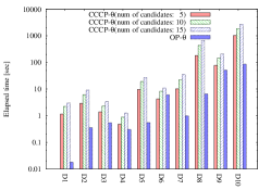
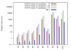
(a) Elapsed time for CCCP and proposed OP (linear, robust SVC)

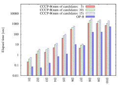
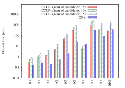
(b) Elapsed time for CCCP and proposed OP (RBF, robust SVC)

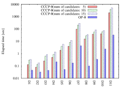
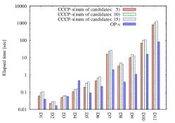
(c) Elapsed time for CCCP and proposed OP (linear, robust SVR)

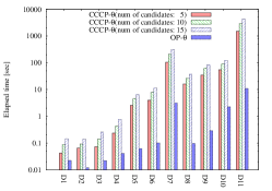
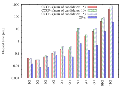
(d) Elapsed time for CCCP and proposed OP (RBF, robust SVR)

Figure 6: Elapsed time when the number of ($\theta,s$)-candidates is increased. Changing the number of hyper-parameter candidates affects the computation time of CCCP, but not OP because the entire path of solutions is computed with the infinitesimal resolution.

5.3 Computation Time

Finally, we compared the computational costs of the entire model-building process of each method. The results are shown in Figure 6. Note that the computational cost of the OP algorithm does not depend on the number of hyper-parameter candidates of $\theta$ or $s$, because the entire path of local solutions has already been computed with the infinitesimal resolution in the homotopy computation. On the other hand, the computational cost of CCCP depends on the number of hyper-parameter candidates. In our implementation of CCCP, we used the warm-start approach, i.e., we initialized CCCP with the previous solution for efficiently computing a sequence of solutions. The results indicate that the proposed OP algorithm enables stable and efficient control of robustness, while CCCP suffers a trade-off between model selection performance and computational costs.

6 Conclusions

In this paper, we proposed a novel robust SVM learning algorithm based on the homotopy approach that allows efficient computation of the sequence of local optimal solutions when the influence of outliers is gradually emphasized. The algorithm is built on our theoretical findings about the geometric property and the optimality conditions of local solutions of robust SVM. Experimental results indicate that our algorithm tends to find better local solutions possibly due to the simulated annealing-like effect and the stable control of robustness. One of the important future works is to adopt scalable homotopy algorithms [28] or approximate parametric programming algorithms [34] for further improving the computational efficiency.

Appendix A Proof of Theorem 3

Although $f^{*}_{{\cal P}}$ is a feasible solution, it is not a local optimum for $\theta\in[0,1)$ and $s\leq 0$ because

$$\alpha_{i}\leq C\theta i\in\tilde{{\cal I}}\cap{\cal O},$$ for (28a)

$$\alpha_{i}\geq C i\in\tilde{{\cal O}}\cap{\cal I},$$ for (28b)

violate the KKT conditions (16) for $\tilde{{\cal P}}$. These feasibility and sub-optimality indicates that

$$J_{\tilde{{\cal P}}}(f^{*}_{\tilde{{\cal P}}};\theta)<J_{{\cal P}}(f^{*}_{{\cal P}};\theta),$$ (29)

we arrive at (18). Q.E.D.

Appendix B Proof of Theorem 4

Sufficiency: If (19e) is true, i.e., if there are NO instances with $y_{i}f^{*}_{\cal P}(\mbox{\boldmath$x$}_{i})=s$, then any convex problems defined by different partitions $\tilde{{\cal P}}\neq{\cal P}$ do not have feasible solutions in the neighborhood of $f^{*}_{\cal P}$. This means that if $f^{*}_{\cal P}$ is a conditionally optimal solution, then it is locally optimal. (19a)-(19d) are sufficient for $f^{*}_{\cal P}$ to be conditionally optimal for the given partition ${\cal P}$. Thus, (19) is sufficient for $f^{*}_{\cal P}$ to be locally optimal.

Necessity: From Theorem 3, if there exists an instance such that $y_{i}f^{*}_{\cal P}(\mbox{\boldmath$x$}_{i})=s$, then $f^{*}_{\cal P}$ is a feasible but not locally optimal. Then (19e) is necessary for $f^{*}_{\cal P}$ to be locally optimal. In addition, (19a)-(19d) are also necessary for local optimality, because of every local optimal solutions are conditionally optimal for the given partition ${\cal P}$. Thus, (19) is necessary for $f^{*}_{\cal P}$ to be locally optimal.

Q.E.D.

Appendix C Implementation of D-step

In D-step, we work with the following convex problem

$$f^{*}_{\tilde{{\cal P}}}:=\mathop{\rm argmin}\limits_{f\in{\rm pol}(\tilde{{\cal P}};s)}J_{\tilde{{\cal P}}}(f;\theta).$$ (30)

where, $\tilde{{\cal P}}$ is updated from ${\cal P}$ as (17).

Let us define a partition $\Pi:=\{{\cal R},{\cal E},{\cal L},\tilde{{\cal I}}^{\prime},\tilde{{\cal O}}^{\prime},\hat{{\cal O}}^{\prime\prime}\}$ of $\mathbb{N}_{n}$ such that

$$i\in{\cal R} \Rightarrow y_{i}f(\bm{x}_{i})>1,$$ (31a)

$$i\in{\cal E} \Rightarrow y_{i}f(\bm{x}_{i})=1,$$ (31b)

$$i\in{\cal L} \Rightarrow s<y_{i}f(\bm{x}_{i})<1,$$ (31c)

$$i\in\tilde{{\cal I}}^{\prime} \Rightarrow y_{i}f(\bm{x}_{i})=s\text{ and }i\in\tilde{{\cal I}},$$ (31d)

$$i\in\tilde{{\cal O}}^{\prime} \Rightarrow y_{i}f(\bm{x}_{i})=s\text{ and }i\in\tilde{{\cal O}},$$ (31e)

$$i\in\tilde{{\cal O}}^{\prime\prime} \Rightarrow y_{i}f(\bm{x}_{i})<s.$$ (31f)

If we write the conditionally optimal solution as

$$f^{*}_{\tilde{{\cal P}}}(x):=\sum_{j\in\mathbb{N}_{n}}\alpha_{j}^{*}y_{j}K(x,\bm{x}_{j}),$$ (32)

$\{\alpha^{*}_{j}\}_{j\in\mathbb{N}_{n}}$ must satisfy the following KKT conditions

$$y_{i}f^{*}_{\tilde{{\cal P}}}(\mbox{\boldmath$x$}_{i})>1~{} \Rightarrow~{}\alpha_{i}^{*}=0$$ (33a)

$$y_{i}f^{*}_{\tilde{{\cal P}}}(\mbox{\boldmath$x$}_{i})=1~{} \Rightarrow~{}\alpha_{i}^{*}\in[0,C],$$ (33b)

$$s<y_{i}f^{*}_{\tilde{{\cal P}}}(\mbox{\boldmath$x$}_{i})<1~{} \Rightarrow~{}\alpha_{i}^{*}=C$$ (33c)

$$y_{i}f^{*}_{\tilde{{\cal P}}}(\mbox{\boldmath$x$}_{i})=s,i\in\tilde{{\cal I}}^{\prime}~{} \Rightarrow~{}\alpha_{i}^{*}\geq C,$$ (33d)

$$y_{i}f^{*}_{\tilde{{\cal P}}}(\mbox{\boldmath$x$}_{i})=s,i\in\tilde{{\cal O}}^{\prime}~{} \Rightarrow~{}\alpha_{i}^{*}\leq C\theta,$$ (33e)

$$y_{i}f^{*}_{\tilde{{\cal P}}}(\mbox{\boldmath$x$}_{i})<s,i\in\tilde{{\cal O}}^{\prime\prime}~{} \Rightarrow~{}\alpha_{i}^{*}=C\theta.$$ (33f)

At the beginning of the D-step, $f^{*}_{\tilde{{\cal P}}}(\bm{x}_{i})$ violates the KKT conditions by

$$\Delta f_{i}:=y_{i}\left[\begin{array}[]{cc}\bm{K}_{i,\Delta_{{\cal I}\to{\cal O}}}&\bm{K}_{i,\Delta_{{\cal O}\to{\cal I}}}\\ \end{array}\right]\left[\begin{array}[]{c}\bm{\alpha}^{\rm(bef)}_{\Delta_{{\cal I}\to{\cal O}}}-\mathbf{1}C\theta\\ \bm{\alpha}^{\rm(bef)}_{\Delta_{{\cal O}\to{\cal I}}}-\mathbf{1}C\end{array}\right].$$

where $\bm{\alpha}^{(\rm bef)}$ is the corresponding $\bm{\alpha}$ at the beginning of the D-step, while $\Delta_{{\cal I}\to{\cal O}}$ and $\Delta_{{\cal O}\to{\cal I}}$ denote the difference in $\tilde{{\cal P}}$ and ${\cal P}$ defined as

$$\Delta_{{\cal I}\to{\cal O}} :=\{i\in{\cal I}~{}|~{}y_{i}f_{{\cal P}}(\bm{x}_{i})=s\},$$

$$\Delta_{{\cal O}\to{\cal I}} :=\{i\in{\cal O}~{}|~{}y_{i}f_{{\cal P}}(\bm{x}_{i})=s\}.$$

Then, we consider the following another parametrized problem with a parameter $\mu\in[0,1]$:

$$f_{\tilde{{\cal P}}}(\bm{x}_{i};\mu):=f_{\tilde{{\cal P}}}(\bm{x}_{i})+\mu\Delta f_{i}~{}\forall~{}i\in\mathbb{N}_{n}.$$

In order to always satisfy the KKT conditions for $f_{\tilde{{\cal P}}}(\bm{x}_{i};\mu)$, we solve the following linear system

$$\bm{Q}_{{\cal A},{\cal A}}\left[\begin{array}[]{c}\bm{\alpha}_{{\cal E}}\\ \bm{\alpha}_{\tilde{{\cal I}}^{\prime}}\\ \bm{\alpha}_{\tilde{{\cal O}}^{\prime}}\end{array}\right]=\left[\begin{array}[]{c}\bm{1}\\ \bm{s}\\ \bm{s}\end{array}\right]-\bm{Q}_{{\cal A},{\cal L}}\mathbf{1}C-\bm{Q}_{{\cal A},\tilde{{\cal O}}^{\prime\prime}}\mathbf{1}C\theta$$

$$-\left[\begin{array}[]{cc}\bm{Q}_{{\cal A},\Delta_{{\cal I}\to{\cal O}}}&\bm{Q}_{{\cal A},\Delta_{{\cal O}\to{\cal I}}}\\ \end{array}\right]\left[\begin{array}[]{c}\bm{\alpha}^{\rm(bef)}_{\Delta_{{\cal I}\to{\cal O}}}-\mathbf{1}C\theta\\ \bm{\alpha}^{\rm(bef)}_{\Delta_{{\cal O}\to{\cal I}}}-\mathbf{1}C\end{array}\right]\mu,$$

where ${\cal A}:=\{{\cal E},\tilde{{\cal I}}^{\prime},\tilde{{\cal O}}^{\prime}\}$. This linear system can also be solved by using the piecewise-linear parametric programming while the scalar parameter $\mu$ is continuously moved from 1 to 0.

In this parametric problem, we can show that $f^{*}_{\tilde{{\cal P}}}(\bm{x}_{i};\mu)=f^{*}_{{\cal P}}(\bm{x}_{i})$ if $\mu=1$ and $f^{*}_{\tilde{{\cal P}}}(\bm{x}_{i};\mu)=f^{*}_{\tilde{{\cal P}}}(\bm{x}_{i})$ if $\mu=0$ for all $i\in\mathbb{N}_{n}$.

Since the number of elements in $\Delta_{{\cal I}\to{\cal O}}$ and $\Delta_{{\cal O}\to{\cal I}}$ are typically small, the D-step can be efficiently implemented by a technique used in the context of incremental learning [33].

References

- [1] B. E. Boser, I. M. Guyon, and V. N. Vapnik, “A training algorithm for optimal margin classifiers,” Proceedings of the Fifth Annual ACM Workshop on Computational Learning Theory, pp. 144–152, 1992.
- [2] C. Cortes and V. Vapnik, “Support-vector networks,” Machine Learning, vol. 20, pp. 273–297, 1995.
- [3] V. N. Vapnik, Statistical Learning Theory. Wiley Inter-Science, 1998.
- [4] X. Zhu, Z. Ghahramani, and J. Lafferty, “Semi-supervised learning using gaussian fields and harmonic functions,” in ICML, vol. 3, 2003, pp. 912–919.
- [5] X. Zhu, “Semi-supervised learning literature survey,” 2005.
- [6] M. C. Yuen, I. King, and K. S. Leung, “A survey of crowdsourcing systems,” in Privacy, Security, Risk and Trust (PASSAT) and 2011 IEEE Third Inernational Conference on Social Computing (SocialCom), 2011 IEEE Third International Conference on. IEEE, 2011, pp. 766–773.
- [7] K. Mao, L. Capra, M. Harman, and Y. Jia, “A survey of the use of crowdsourcing in software engineering,” RN, vol. 15, p. 01, 2015.
- [8] H. Masnadi-Shiraze and N. Vasconcelos, “Functional gradient techniques for combining hypotheses,” in Advances in Large Margin Classifiers. MIT Press, 2000, pp. 221–246.
- [9] X. Shen, G. Tseng, X. Zhang, and W. H. Wong, “On -learning,” Journal of the American Statistical Association, vol. 98, no. 463, pp. 724–734, 2003.
- [10] N. Krause and Y. Singer, “Leveraging the margin more carefully,” in Proceedings of the 21st International Conference on Machhine Learning, 2004, pp. 63–70.
- [11] Y. Liu, X. Shen, and H. Doss, “Multicategory -learning and support vector machine: Computational tools,” Journal of Computational and Graphical Statistics, vol. 14, pp. 219–236, 2005.
- [12] Y. Liu and X. Shen, “Multicategory -learning,” Journal of the American Statistical Association, vol. 101, p. 98, 2006.
- [13] L. Xu, K. Crammer, and D. Schuurmans, “Robust support vector machine traiing via convex outlier ablation,” in Proceedings of the National Conference on Artificial Intelligence (AAAI), 2006.
- [14] R. Collobert, F. Sinz, J. Weston, and L. Bottou, “Trading convexity for scalability,” in Proceedings of the 23rd International Conference on Machine Learning, 2006, pp. 201–208.
- [15] Y. Wu and Y. Liu, “Robust truncated hinge loss support vector machines,” Journal of the American Statistical Association, vol. 102, pp. 974–983, 2007.
- [16] H. Masnadi-Shirazi and N. Vasconcelos, “On the design of loss functions for classification: theory, robustness to outliers, and savageboost,” in Advances in Neural Information Processing Systems, vol. 22, 2009, pp. 1049–1056.
- [17] Y. Freund, “A more robust boosting algorithm,” arXiv:0905.2138, 2009.
- [18] Y. Yu, M. Yang, L. Xu, M. White, and D. Schuurmans, “Relaxed clipping: a global training method for robust regression and classification,” in Advances in Neural Information Processing Systems, vol. 23, 2010.
- [19] J. Hromkovic, Algorithmics for Hard Problems. Springer, 2001.
- [20] E. L. Allgower and K. George, “Continuation and path following,” Acta Numerica, vol. 2, pp. 1–63, 1993.
- [21] T. Gal, Postoptimal Analysis, Parametric Programming, and Related Topics. Walter de Gruyter, 1995.
- [22] K. Ritter, “On parametric linear and quadratic programming problems,” mathematical Programming: Proceedings of the International Congress on Mathematical Programming, pp. 307–335, 1984.
- [23] M. J. Best, “An algorithm for the solution of the parametric quadratic programming problem,” Applied Mathemetics and Parallel Computing, pp. 57–76, 1996.
- [24] A. L. Yuille and A. Rangarajan, “The concave-convex procedure (cccp),” in Advances in Neural Information Processing Systems, vol. 14, 2002.
- [25] S. Suzumura, K. Ogawa, M. Sugiyama, and I. Takeuchi, “Outlier path: A homotopy algorithm for robust svm,” in Proceedings of the 31st International Conference on Machine Learning (ICML-14), 2014, pp. 1098–1106.
- [26] C. H. Zhang, “Nearly unbiased variable selection under minimax concave penalty,” Annals of Statistics, vol. 38, pp. 894–942, 2010.
- [27] R. Mazumder, J. H. Friedman, and T. Hastie, “Sparsenet: coordinate descent with non-convex penalties,” Journal of the American Statistical Association, vol. 106, pp. 1125–1138, 2011.
- [28] H. Zhou, A. Armagan, and D. B. Dunson, “Path following and empirical Bayes model selection for sparse regression,” arXiv:1201.3528, 2012.
- [29] K. Ogawa, M. Imamura, I. Takeuchi, and M. Sugiyama, “Infinitesimal annealing for training semi-supervised support vector machines,” in Proceedings of the 30th International Conference on Machine Learning, 2013.
- [30] S. Boyd and L. Vandenberghe, Convex Optimization. Cambridge University Press, 2004.
- [31] D. DeCoste and K. Wagstaff, “Alpha seeding for support vector machines,” in Proceeding of the Sixth ACM SIGKDD International Conference on Knowledge Discovery and Data Mining, 2000.
- [32] T. Hastie, S. Rosset, R. Tibshirani, and J. Zhu, “The entire regularization path for the support vector machine,” Journal of Machine Learning Research, vol. 5, pp. 1391–415, 2004.
- [33] G. Cauwenberghs and T. Poggio, “Incremental and decremental support vector machine learning,” in Advances in Neural Information Processing Systems, 2001, vol. 13, pp. 409–415.
- [34] J. Giesen, M. Jaggi, and S. Laue, “Approximating parameterized convex optimization problems,” ACM Transactions on Algorithms, vol. 9, 2012.