Top-forms of Leading Singularities in Nonplanar Multi-loop Amplitudes

Abstract

The on-shell diagram is a very important tool in studying scattering amplitudes. In this paper we discuss the on-shell diagrams without external BCFW-bridges. We introduce an extra step of adding an auxiliary external momentum line. Then we can decompose the on-shell diagrams by removing external BCFW-bridges to a planar diagram whose top-form is well-known to all now. The top-form of the on-shell diagram with the auxiliary line can be obtained by adding the BCFW-bridges in an inverse order as discussed in our former paper Chen:2014ara . To get the top-form of the original diagram, the soft limit of the auxiliary line is needed. We obtain the evolution rule for the Grassmannian integral and the geometry constraint under the soft limit. This completes the top-form description of leading singularities in nonplanar scattering amplitudes of $\mathcal{N}=4$ Super Yang-Mills (SYM), which is valid for arbitrary higher-loops and beyond the Maximally-Helicity-Violation (MHV) amplitudes.

1 Introduction

Bipartite diagrams and the associated Grassmannian geometry 2006math……9764P ; GeometryOnshell have recently found their way into the scattering amplitude studies. An amazing discovery was to exploit them in computing scattering amplitudes in $\mathcal{N}=4$ SYM theory NimaGrass ; NimaSMatrix ; Paulos2014 ; BaiHe2014 ; Bargheer:2014mxa ; Ferro2014gca ; Franco2014csa ; Elvang2014fja . Planar scattering amplitudes are represented by on-shell bipartite diagrams and expressed in “top-form” as contour integrations over the Grassmannian submanifolds. Planar loop integrands in $\mathcal{N}=4$ SYM have recently been constructed in NimaGrass ; arkani2012local along with the introduction of the Grassmannian and on-shell method. As a result, the “$d$log” form and the Yangian symmetry 2010JHEP…04..085B ; Broedel1403 ; Broedel2014 ; Beisert ; Chicherin2014 of the scattering amplitudes are made manifest in the planar limit. It is natural to extend the construction to non-planar scattering amplitudes Chen:2014ara ; Bern:2014kca ; Arkani-Hamed:2014bca ; Franco:2015rma , and theories of reduced (super) symmetries Bidder2005N1 ; neitzke2014cluster ; xie2012network .

The leading singularities are represented in the top-form of Grassmannian integrals in which the integrands are comprised of rational functions of minors $\{\mathbf{R}(M_{C})\}$ of the Grassmannian $C$ matrices. The top-form is elegant in that the amplitude structures are simple and compact; and the Yangian symmetry is manifest in the positive diffeomorphisms of positive Grassmannian geometry NimaGrass . It is therefore crucial to express scattering amplitudes in top-form in order to explore its power to further uncover hidden symmetries and dualities of the scattering amplitudes. We present in this letter our successful construction of top-forms for non-planar scattering amplitudes. Our method applies to multi-loop, beyond-MHV leading singularities.

Recently, exciting progress in $\mathcal{N}=4$ SYM scattering amplitude computation (by the on-shell method) is reported by many research groups in Chen:2014ara ; GeometryOnshell ; Bern:2014kca ; Arkani-Hamed:2014bca ; BernNP12 ; du2014permutation ; NimaSin2014 ; franco2015non ; Johansson:2015ava . Together we have made a step forward in the computation of nonplanar $\mathcal{N}=4$ SYM scattering amplitudes, and hopefully in the formulation of AdS/CFT correspondence at finite N.

2 BCFW-bridge decompositions of leading singularities

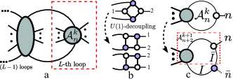
Figure 1: (a) Obtaining the $L$-th loop amplitude recursively. (b) Utilising the $U(1)$ decoupling relation to turn a nonplanar diagram into a planar one. (c) Introduction of an auxiliary external momentum line to form the BCFW bridge.

The aim of this work is to obtain a simple and compact analytical expression of leading singularities of scattering amplitudes, valid for arbitrary number of loops, beyond the planar limit. A general leading singularity can be represented by a reduced on-shell diagram. BCFW-bridge decomposition provides an efficient way of constructing on-shell diagrams in the planar limit. In non-planar cases, we can obtain the BCFW-bridge decomposition chain by extracting planar sub-diagrams and computing them recursively Chen:2014ara as shown in Fig. 2. For the sub-diagrams that are BCFW-decomposible, we follow the recipe presented in Chen:2014ara . There exist, however, “No Bridge” (NB) diagrams which do not contain any BCFW bridges Chen:2014ara ; Arkani-Hamed:2014bca . We have presented a method in Chen:2014ara to transform some NB-diagrams, schematically depicted in Fig. 2 (b), by applying $U(1)$-decoupling relations KK .

In this work we present a general method applicable to any NB-diagrams. The key is to add an auxiliary external momentum line to form an auxiliary BCFW bridge, shown in Fig. 2 (c). To regain the original NB diagram we take the soft limit SoftLimitA ; SoftLimitB ; Volovich:2015yoa ; Klose:2015xoa , setting the auxiliary momentum to zero. This way the BCFW-bridge decomposition chain of the reduced on-shell diagrams beyond the planar limit can be obtained.

In the rest of the letter we present a recipe for constructing an analytical expression, the top-form, for a nonplanar leading singularity using the BCFW-bridge decomposition chain Chen:2014ara after adding an auxiliary external momentum line.

3 Construction of the top-form

The top-form of an on-shell diagram is obtained once the geometric constraints, $\Gamma$, and the integrand, $f(C)$, are determined. A non-planar leading singularity in the form NimaGrass

$$\mathcal{T}=\oint_{\Gamma}{dC^{k\times n}\over\text{Vol}(GL(k))}{\delta^{k\times 4}(C\cdot\widetilde{\eta})\over f(C)}\delta^{k\times 2}(C\cdot\widetilde{\lambda})\delta^{2\times(n-k)}(\lambda\cdot C^{\perp})~{}.\vspace{-5pt}$$

requires to calculate $f(C)$ and $\Gamma$ under the BCFW shifts and take soft limit of the auxiliary BCFW bridges.

Let us study the BCFW shifts. The integrand, $f(C)$, must contain those poles equivalent to the constraints in $\Gamma$; otherwise the contour integration around $\Gamma$ will vanish. Each BCFW bridge removes one pole in $f(C)$ by shifting a zero minor to be nonzero: in general the poles in the integrand must change their forms and the integrand changes its functional form accordingly. To see this we parametrize the constraint matrix, $C$, using the BCFW parameter, $\alpha$. In a BCFW shift, a column vector $X$ is shifted: $X\rightarrow\widehat{X}=X+\alpha Y,$ with several minors of $f(C)$ become functions of $\alpha$. After the shift, there exists at least one constraint $M_{0}(X)=0$ being shifted to $M_{0}(\widehat{X})=M_{0}(X)+\alpha R(Y)$ if there is a top-form. This is demonstrated in the following section. Meanwhile the factor $M_{0}(\widehat{X})$ should be present in the dominator to contribute a pole at $\alpha=0$. In other words $\alpha=M_{0}(\widehat{X})/R(Y)$ is then a rational function of $\widehat{C}$ and can be subtracted from other shifted minors to obtain some shift-invariant minors of $\widehat{C}$, $M_{i}(X)=M_{i}(\widehat{X}-\alpha Y).$ In summary, attaching a BCFW bridge, the integrand is,

$$f(\widehat{C})=M_{0}(\widehat{X})\prod_{i}M_{i}(\widehat{X}-\alpha Y)\times\left(\begin{array}[]{c}\text{minors}\\ \text{without}~{}\alpha\end{array}\right).\vspace{-5pt}$$ (1)

3.1 An MHV example

A six-point three-loop MHV example have been analyzed in Arkani-Hamed:2014bca . Here, for comparison, we provide our calculation by attaching the auxiliary BCFW-bridges. We attach an auxiliary external momentum line, in Fig. 2,

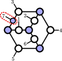
Figure 2: An MHV example

and form an auxiliary BCFW-bridge $(3,7)$. This on-shell diagram can be decomposed to identity as follows, $(1,7)\rightarrow(2,6)\rightarrow(3,5)\rightarrow(2,3)\rightarrow(3,4)\rightarrow(12)\rightarrow(2,3)\rightarrow(5,7)\rightarrow(3,7)$. Before adding Bridge-$(5,7)$, the on-shell diagram is still planar. The Grassmannian constraints and the top-form can be obtained directly from the permutation NimaGrass shown in the first row of Tab.1. Adding Bridge-$(5,7)$, the constraint $(7,1)^{1}\rightarrow(1,5,7)^{2}$, as shown in the second row of Tab.1. Here we use $(i_{1},i_{2},\cdots,i_{m})^{r}$, where $m,r$ are positive integrals, to denote the matrix of rank $r$ constructed by the columns $i_{1},\cdots,i_{m}$ in the $C$ matrix. $(i_{1},i_{2},\cdots,i_{m})^{r}$ also characterize the $(r-1)$-dimensional hyperplane in the $k$-dimensional projective space. Adding Bridge-$(3,7)$, the constraint $(1,5,7)^{2}$ disappears.

Table 1: The evolution of the geometric constraints.

	$(7,1)^{1}$	$(2,3,4)^{2}$	$(4,5,6)^{2}$	$(6,1,2)^{2}$
$(5,7)$	$(1,5,7)^{2}$	$(2,3,4)^{2}$	$(4,5,6)^{2}$	$(1,2,6)^{2}$
$(3,7)$		$(2,3,4)^{2}$	$(4,5,6)^{2}$	$(1,2,6)^{2}$

Before attaching Bridge-$(5,7)$, the top-form is

$$\frac{1}{(123)(234)(345)(456)(567)(671)(712)},$$

where we use $(i_{1}i_{2}\cdots i_{k})$ to denote the minor of the matrix which is formed by the columns $i_{1}\cdots i_{k}$ in $C$. When attaching $(5,7)$, the contour integral around the pole $(712)=(\widehat{7}12)-\alpha(512)$ is replaced by $d\alpha\over\alpha$ with $\alpha=\frac{(\widehat{7}12)}{(512)}$. All the minors with column $7$ except $(712)$ are affected by the bridge

$$\begin{array}[]{ccccc}(567)&\rightarrow&{(56(\widehat{7}5)\cap(12))\over(512)}&=&(56\widehat{7})\\ (671)&\rightarrow&{(6(\widehat{7}5)\cap(12)1)\over(512)}&=&\frac{(\widehat{7}15)(126)}{(512)},\end{array}$$

where the $(\widehat{7}5)\cap(12)$ denotes the intersection point between the two lines characterized by $(\widehat{7}5)$ and $(12)$. Then the top-form integrand becomes

$$\frac{(125)}{(123)(234)(345)(456)(567)(157)(126)(127)}.$$

Similarly after attaching Bridge-$(3,7)$ the top-form integrand becomes

$$\frac{(135)^{2}}{(123)(234)(345)(456)(156)(357)(157)(126)(137)}.$$

To obtain the top-form of the original diagram, we parametrize the ${C^{\prime}}$ as

$$\left(\begin{array}[]{cccccc|c}&&&C&&&0\\ &&&&&&0\\ \hline\cr 0&0&c_{3}&c_{4}&c_{5}&c_{6}&1\\ \end{array}\right).$$

Then we expand all the minors in ${C^{\prime}}$ in terms of those in $C$

$$\begin{array}[]{ll}(126)=(12)c_{6}&(234)=-c_{3}(24)+c_{4}(23)\\ (123)=(12)c_{3}&(456)=c_{4}(56)-c_{5}(46)\\ (156)=-(16)c_{5}&(135)=-c_{3}(15)+c_{5}(13)\\ (137)=(13)&(345)=c_{3}(45)-c_{4}(35)+c_{5}(34)\\ (357)=(35)&(157)=(15)~{}~{}.\end{array}$$

The top-form becomes

$$\frac{(-c_{3}(15)+c_{5}(13))^{2}}{-(12)(35)(15)(12)(13)(16)c_{3}c_{6}c_{5}(-c_{3}(24)+c_{4}(23))}$$

$$\times {1\over(c_{3}(45)-c_{4}(35)+c_{5}(34))(c_{4}(56)-c_{5}(46))}.$$

The additional pole is characterised by $(126),(234),(456)$. The contour integration gives $c_{6}\rightarrow 0,c_{3}\rightarrow\frac{(23)}{(24)}c_{4},c_{5}\rightarrow\frac{(56)}{(46)}c_{4}$ and

$$\frac{[(56)(13)(24)-(23)(15)(46)]^{2}}{(23)(12)(24)(26)(45)(34)(16)(56)(35)(15)(13)(46)}$$

consistent with the MHV example in Arkani-Hamed:2014bca . This can be simplified further,

$$-f_{p}(125364)+f_{p}(125463)-f_{p}(134265)$$

$$+f_{p}(126543)-f_{p}(132465)-f_{p}(123564),$$

with $f_{p}$ denoting the planar amplitudes of the corresponding orders.

4 Construction of the top-from of NB diagram

Now we discuss the new Grassmannian geometry structures in the NB diagrams Chen:2014ara ; Arkani-Hamed:2014bca . For the sub-diagram structure in Fig. 2 (b), the top-form is obtained by imposing $U(1)$-decoupling relation in Chen:2014ara ; in this work we focus on the auxiliary BCFW bridges which is suitable for the general diagrams as shown in Fig. 2 (c). The top-forms of those diagrams containing auxiliary BCFW bridges can be obtained using the above method. We discuss presently how they return to the top-forms of the original NB diagrams upon taking the soft limits.

The on-shell diagram $\mathcal{A}_{n+1}^{k+1}$ with one auxiliary line as shown in Fig.2 (c) can be written in two equivalent forms:

$$\int\frac{d^{2}\lambda_{I}d^{2}\widetilde{\lambda}_{I}d^{4}\widetilde{\eta}_{I}}{vol(GL(1))}\frac{\mathcal{A}_{n+2}^{k+1}\langle I\bar{I}\rangle^{3}}{\left\langle\bar{n}I\right\rangle^{2}\left\langle\bar{I}\bar{n}\right\rangle}\delta([\bar{n}I])\delta^{4}(\widetilde{\eta}_{\bar{n}}+{\langle\bar{I}\bar{n}\rangle\over\langle\bar{I}I\rangle}\widetilde{\eta}_{I}),~{}~{}~{}~{}$$ (2)

$$\oint_{\bar{\Gamma}}{dC^{k\times n}dc_{k+1}\cdots dc_{n}\over\text{Vol}(GL(k))}{(1\cdots k)\over f(C,c_{i})}$$

$$\times\delta^{k\times 4}(C\cdot\widetilde{\eta})\delta^{k\times 2}(C\cdot\widetilde{\lambda})\delta^{2(n-k)}(\lambda\cdot{C^{\prime}}^{\perp})$$

$$\times\delta^{2}(\sum_{i=k+1}^{n}c_{i}\tilde{\lambda}_{i}+c_{\bar{n}}\tilde{\lambda}_{\bar{n}})\delta^{4}(\sum_{i=k+1}^{n}c_{i}\widetilde{\eta}_{i}+c_{\bar{n}}\widetilde{\eta}_{\bar{n}}),$$ (3)

where $c_{\bar{n}}=1$ and $\bar{n}$ denote the index of the auxiliary line. Eq.(2) is obtained directly from Fig.2(c) by integrating over the internal line $\bar{I}$. Eq.(4) is a general top-form of $\mathcal{A}_{n+1}^{k+1}$, where we choose a particular parametrization of the Grassmannian matrix ${C^{\prime}}$ as

$$C^{\prime}=\left(\begin{array}[]{cccccc|c}&&&&&&0\\ &&&C&&&\vdots\\ &&&&&&0\\ \hline\cr 0&\cdots&0&c_{k+1}&\cdots&c_{n}&1\end{array}\right).$$

Our method of adding the auxiliary line can be verified by comparing (2) and (4). Noting that

$$\delta^{2}(\sum_{i=k+1}^{n}c_{i}\tilde{\lambda}_{i}+c_{\bar{n}}\tilde{\lambda}_{\bar{n}})=\delta(\sum_{i=k+1}^{n}c_{i}{[i1]\over[\bar{n}1]}+1)\delta([\bar{n}I]),$$

(2) and (4) can therefore be proved to contain the term

$$\delta([\bar{n}I])\delta^{4}(\widetilde{\eta}_{\bar{n}}+{\langle\bar{I}\bar{n}\rangle\over\langle\bar{I}I\rangle}\widetilde{\eta}_{I}),$$

which can be removed from the overall constraint delta function. The remaining part of (2) corresponds to the NB diagram $\mathcal{A}_{n}^{k}$ in the limit $\lambda_{\bar{n}}\rightarrow 0$. On the other hand, after taking the soft limit (4) yields

$$\mathcal{A}_{n}^{k}=\oint_{\bar{\Gamma}}{dC^{k\times n}dc_{k+1}\cdots dc_{n}\over\text{Vol}(GL(k))}{(1\cdots k)\delta^{k\times 4}(C\cdot\widetilde{\eta})\over f(C,c_{i})}$$

$$\times\delta^{k\times 2}(C\cdot\widetilde{\lambda})\delta^{2\times(n-k)}(\lambda\cdot{C}^{\perp})\delta(\sum_{i=k+1}^{n}c_{i}{[i1]\over[\bar{n}1]}+1)~{}.$$ (4)

This is easily proven by counting the degrees of freedom of the associated on-shell diagram in which only one element $c_{f}$ among $c_{i}$ is a free parameter. As we shall prove in the following section, that a given NB diagram has a top-form requires that $c_{i}/c_{r}=\mathbf{R}(M_{C})$. Using this relation, the integration

$$\int{dc_{r}\over c_{r}}\delta(\sum_{i=k+1}^{n}c_{i}{[i1]\over[\bar{n}1]}+1)$$

gives 1. Finally we obtain the top-form of $\mathcal{A}_{n}^{k}$ by expanding the minors of ${C^{\prime}}$ into $C$ minors in the integrand.

5 Rational top-forms and rational soft limit:

Now we study on which kind of nonplanar on-shell diagrams can have rational top-forms. We address this question by building an equivalent relation between rational top-form and rational soft limit. If the soft limit of auxiliary line leads to additional constraints such that $c_{i}\over c_{j}$ is a rational function of $C$-minors for all non-vanishing $c_{i}$ in the added row of ${C^{\prime}}$, we call this soft limit a rational soft limit.

When the soft limit of the auxiliary line is a rational soft limit, then the NB diagram with auxiliary line has a rational top-form if and only if the original NB diagram has a rational top-form.

We fist consider the free parameters $\alpha$ in the top-form integrand $f(C)$ as shown in Eq. (1). The $C$ matrix parameters $\alpha_{C}$ that can be expressed as by $\mathbf{R}(M_{C})$ is also of the form $\mathbf{R}(M_{C^{\prime}})$. The additional ${C^{\prime}}$ elements $c_{i}$ are of the form $c_{r}\mathbf{R}(\alpha_{C})$ (indicating a rational soft limit for $c_{r}\neq 0$). Since $c_{r}$ is naturally $\mathbf{R}(M_{C^{\prime}})$, all free parameters in ${C^{\prime}}$ are then rational functions of minors, i.e. the top-form is rational. Inversely, given the linear auxiliary bridge and rational soft limit, any $C$ parameter denoted by $\mathbf{R}(M_{C^{\prime}})$ can be expanded as $\mathbf{R}(M_{C})$ directly according to the procedure above.

Then let us study the geometry constraints. Geometry constraints are linear relations among columns of the $C$ matrix. In fact, the total space is taken as the $(k-1)$-dimensional projective space. Each column labeled by the index of the external line can be mapped to a point in the projective space. For the diagram which can be constructed by attaching BCFW bridges, the constraints are all coplanarity constraints for the points of external legs Chen:2014ara . For the NB diagrams, after attaching the auxiliary lines, the geometry constraints in $C^{\prime}$ are still coplanarity constraints. Hence we only need to discuss how the geometry constraints evolve in the rational soft limit.

The simplest case is that the geometry constraints in $C^{\prime}$ are all untangled. Then the coplanarity constraints are of the form

$$(i_{1},i_{2},\cdots,i_{m})^{m-1}.$$

If one of the indices, e. g. $i_{m}$, in the above constraint denotes the auxiliary line, then the geometry constraint becomes $(i_{1},i_{2},\cdots,i_{m-1})^{m-2}$ in the soft-limit. If none of the indices denotes the auxiliary line, then the geometry is invariant for $m<k$. Since $k\rightarrow k-1$ in the soft limit, the geometry constraints for $m=k$ do not exist any more.

In general the geometry constraints are still coplanarity constraints in the soft-limit. However, this is not obvious for the tangled cases. We will leave the explanation of the soft limit behavior for tangled geometry, e. g. $((i_{1}i_{2}\bigcap i_{3}i_{4}),i_{5},\cdots,i_{m})^{r}$, to future work. For now we focus on the algebraic form of these geometry constraints, which is enough to obtain the top-form.

In a general case, the geometry constraints in $C^{\prime}$ can be expanded as

$$F^{\prime}_{1} = \sum_{i=k+1}^{n}c_{i}F_{1}^{c_{i}},~{}~{}F^{\prime}_{2}=\sum_{i=k+1}^{n}c_{i}F_{1}^{c_{i}},$$ (5)

$$\cdots ~{}~{}~{}~{}~{}~{}~{}~{}~{}~{}~{}F^{\prime}_{n-k-1}=\sum_{i=k+1}^{n}c_{i}F_{n-k-1}^{c_{i}},$$

$$\cdots ~{}~{}~{}~{}~{}~{}~{}~{}~{}~{}~{}~{}~{}~{}~{}~{}~{}F^{\prime}_{S}=\sum_{i=k+1}^{n}c_{i}F_{S}^{c_{i}},$$

where $S$ is an integer. There are no higher order terms with respect to $c_{i}$’s. In fact if there are higher order terms, they can be factorized into linear polynomials either with rational minors of $C$ as coefficients or with non-rational minors. For the former case, one of the linear polynomials can be redefined as the geometry constraints. For the latter case, some $c_{i}/c_{j}$ are non-rational, which is beyond the scope of this paper.

Among the constraints in Eq. 5, we can choose arbitrary $n-k-1$ equations to solve for the $c_{i}/c_{r}$. For other equations, we can substitute the solutions of $c_{i}/c_{r}$ to get all the geometry constraints for $C$ after taking the soft limit.

6 More Examples

6.1 An $\overline{\text{MHV}}$ example

In this subsection we give an example of a different situation using an $\overline{\text{MHV}}$ example (Fig.3) for illustration an auxiliary line connected to a white vertex. Attaching an auxiliary line enables the BCFW-decomposition to identity by the following chain: $(7,3)\rightarrow(7,5)\rightarrow(3,4)\rightarrow(2,3)\rightarrow(4,5)\rightarrow(3,4)\rightarrow(1,3)\rightarrow(4,6)\rightarrow(3,7)$. Before adding Bridge-$(7,5)$ the on-shell diagram is planar. The Grassmannian constraints (the first row of Tab.2) and the top-form can be obtained directly from the permutation NimaGrass :

$$\frac{1}{(1234)(2345)(3456)(4567)(5671)(6712)(7123)}.$$

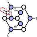
Figure 3: An $\overline{\text{MHV}}$ example

Table 2: Geometry constraints evolution for $\overline{\text{MHV}}$ example

	$(2,(3,4,5)^{2},6)^{3}$	$(3,4,5)^{2}$	$(5,6,7,1)^{3}$	$(7,1,2,3)^{3}$
$(7,5)$	$(2,3,4,6)^{3}$	$(3,4,5,7)^{3}$	$(5,6,7,1)^{3}$	$(7,1,2,3)^{3}$
$(7,3)$		$(3,4,5,7)^{3}$	$(5,6,7,1)^{3}$	$(7,1,2,3)_{3}$

The transformation of constraints after adding the bridges $(7,5)$ and $(7,3)$ is shown in the second and third rows of Tab.2. The top-form of $\mathcal{A}_{7}^{4}$ becomes:

$$\frac{-(2467)^{2}}{(2347)(1246)(2456)(3457)(2346)(4567)(1567)(1267)(1237)}.$$

Without loss of generality, we choose the first four columns of $\widehat{C}$ matrix as identity:

$$\bordermatrix{&\bf{e}_{1}&\bf{e}_{2}&\bf{e}_{3}&\bf{e}_{4}&&&\vec{c}\cr&1&0&0&0&*&*&c_{1}\cr&0&1&0&0&*&*&c_{2}\cr&0&0&1&0&*&*&c_{3}\cr&0&0&0&1&*&*&c_{4}\cr}.$$

Then the last column can be represented by these four columns as:

$$\vec{c}=c_{1}{\bf{e}}_{1}+c_{2}{\bf{e}}_{2}+c_{3}{\bf{e}}_{3}+c_{4}{\bf{e}}_{4}.$$

This way we can rewrite the minor with column-7 as:

$$\begin{array}[]{ll}(1237)=c_{4}(1234)&(1567)=c_{2}(1256)+c_{3}(1356)\\ (1267)=c_{3}(1263)&(2467)=c_{1}(2461)+c_{3}(2463)\\ (2347)=c_{1}(1243)&(3457)=-c_{1}(1345)-c_{2}(2345)\\ \lx@intercol\hfil(4567)=-c_{1}(1456)-c_{2}(2456)-c_{3}(3456)\hfil\lx@intercol\end{array}.$$

Consider the three poles of $\mathcal{A}_{7}^{4}$, since there is no constraint in the top-form of $\mathcal{A}_{6}^{4}$, we should integrate around all of the three poles and remove three coefficients. At last, there is only one coefficient left and others can be represented by it: $c_{4}\rightarrow 0,c_{1}\rightarrow-\frac{(2345)}{(1345)}c_{2},c_{3}\rightarrow-\frac{(1256)}{(1356)}c_{2}.$ The remaining coefficient in the top-form is $\frac{dc_{2}}{c_{2}}$ and can be fixed by one of the columns in $\widehat{C}^{\perp}$ (noting that $\widehat{C}^{\perp}$ has one more column than $C^{\perp}$, which can be removed directly). Finally, the top-form of $\mathcal{A}_{6}^{4}$ is:

$${1\over f_{p}}\frac{-[(2345)(1246)(1356)-(1256)(2346)(1345)]^{2}}{(1246)(2456)(1345)(2346)(1356)(1235)},$$

where $f_{p}=(1234)(2345)(3456)(4561)(5612)(6123)$. This can also be simplified as

$$- f_{p}(142356)-f_{p}(143265)+f_{p}(132456)$$

$$- f_{p}(132654)+f_{p}(123465)-f_{p}(123465).$$

6.2 An NMHV NB diagram example:

In this subsection we present the details in the calculation and simplification in the NMHV example (Fig.4).

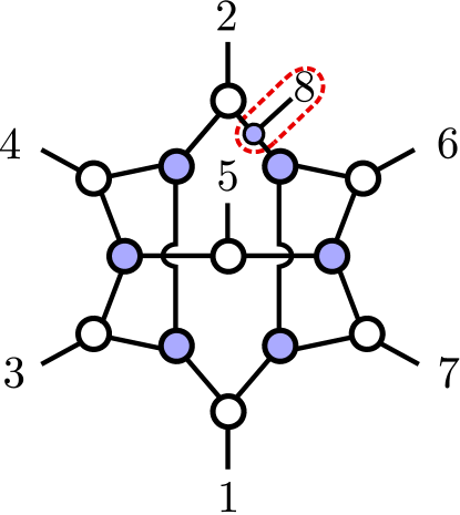
Figure 4: A non-planar NMHV 4-loop leading singularity.

Since this diagram cannot be decomposed by BCFW-bridges directly we introduce an auxiliary external momentum line the leg-8. The diagram transforms to a planar one by removing the bridges $(2,8)$, $(6,8)$ and $(4,2)$. The total decomposition chain is $(2,8)\rightarrow(6,8)\rightarrow(4,2)\rightarrow(1,2)\rightarrow(2,3)\rightarrow(2,4)\rightarrow(4,5)\rightarrow(4,6)\rightarrow(6,7)\rightarrow(1,6)\rightarrow(6,8).$

Before adding Bridge-$(4,2)$ the planar diagram top-form is

$$1\over(1234)(2345)(3456)(4567)(5678)(6781)(7812)(8123)$$

with constraints shown in the first row of Tab. 3.

Table 3: Geometry constraints evolution for NMHV example

	$(1,2,3)^{2}$	$(3,4,5)^{2}$	$(5,6,7)^{2}$	$(7,8,1)^{2}$
$(4,2)$	$(1,2,3,4)^{3}$	$(3,4,5)^{2}$	$(5,6,7)^{2}$	$(7,8,1)^{2}$
$(6,8)$	$(1,2,3,4)^{3}$	$(3,4,5)^{2}$	$(5,6,7)^{2}$	$(6,7,8,1)^{3}$
$(2,8)$	$(1,2,3,4)^{3}$	$(3,4,5)^{2}$	$(5,6,7)^{2}$

After attaching all the BCFW bridges, we obtain the top-form integrand

$${1\over(1234)(2345)(3456)(4567)(1567)(8672)(6781)}$$ (6)

$$\times \frac{(1347)(6721)^{3}}{(7812)(3167)(1237)(1247)(1286)},$$

with geometry constraints as shown in the last row of Tab.3. Then we expand the rank-4 minors into rank-3 minors

$$\begin{array}[]{ll}(1234)=(123)c_{4}&(2345)=-(235)c_{4}+(234)c_{5}\\ (1237)=(123)c_{7}&(3167)=-(317)c_{6}+(316)c_{7}\\ (1286)=-(126)&(6721)=-(721)c_{6}+(621)c_{7}\\ (8672)=-(672)&(3456)=(356)c_{4}-(346)c_{5}\\ (6781)=-(671)&(1347)=-(137)c_{4}+(134)c_{7}\\ (7812)=(712)&(1247)=-(127)c_{4}+(124)c_{7}\\ \lx@intercol\hfil(1567)=(167)c_{5}-(157)c_{6}+(156)c_{7}\hfil\lx@intercol\\ \lx@intercol\hfil(4567)=(467)c_{5}-(457)c_{6}+(456)c_{7}\hfil\lx@intercol.\\ \end{array}$$

Solving all the additional constraints inherited from the auxiliary line and the attached vertex, we get $c_{4}\rightarrow 0,c_{5}\rightarrow 0,c_{7}\rightarrow\frac{(457)}{(456)}c_{6}$ and the final top-form intergrand

$${1\over f_{p}}\frac{(134)(357)[(457)(126)-(456)(127)]^{3}}{(124)(126)(135)(145)(267)(367)(457)^{2}},$$

where $f_{p}=(123)(234)(345)(456)(567)(671)(712)$. Using the Pluker relations the integrand $1\over f(C)$ is

$${(125)\over(124)(126)(167)(235)(257)(143)(345)(567)}$$ (7)

$$+ {(125)\over(124)(127)(165)(235)(267)(143)(345)(567)}$$

$$+ {(125)\over(123)(126)(167)(234)(145)(257)(345)(567)}$$

$$+ {(125)\over(123)(127)(165)(234)(145)(267)(345)(567)}.$$

It is hard to simplify the form further by using the Plüker relations directly. A simpler technique is to para-metrize the $C$ matrix as

$$\bordermatrix{&1&2&3&4&5&6&7\cr&*&*&*&*&0&*&*\cr&*&*&*&*&0&*&*\cr&c_{1}&c_{2}&c_{3}&0&1&0&c_{7}\cr}$$

and expand the three-column minors in the two-column minors. Then the first term in (7) can be written as

$${-(12)(36)\over(124)(126)c_{7}(16)(23)(27)c_{3}(14)(34)(67)(36)}$$ (8)

$$= {-1\over(124)(126)(27)c_{3}(14)(34)(67)c_{7}(36)}$$

$$+ {1\over(124)(126)c_{7}(16)(37)c_{3}(24)(34)(67)}$$

$$= {-1\over(124)(126)(257)(134)(345)(567)(367)}$$

$$- {1\over(124)(126)(167)(234)(357)(345)(567)}.$$

Similarly we can rewrite the second term to forth term in (7) as

$$(II) = {1\over(124)(127)(167)(346)(235)(345)(567)}$$ (9)

$$+ {1\over(124)(127)(134)(267)(356)(345)(567)};$$

$$(III) = {1\over(123)(126)(143)(467)(275)(345)(567)}$$ (10)

$$+ {1\over(123)(126)(243)(467)(175)(345)(567)};$$

$$(IV) = {1\over(123)(127)(143)(267)(456)(345)(567)}$$ (11)

$$+ {1\over(123)(127)(234)(167)(456)(345)(567)}.$$

6.3 An on-shell diagram with two auxiliary lines

Our method can also deal with the on-shell diagrams to which we need add more than one auxiliary lines. We consider the diagram in Fig. 5 where $k=4$ and $n=10$. After attaching the BCFW bridges recursively

$$(C8) \rightarrow (A8)\rightarrow(62)\rightarrow(42)\rightarrow(34)\rightarrow(23)\rightarrow(12)\rightarrow(45)$$

$$\rightarrow (34)\rightarrow(46)\rightarrow(37)\rightarrow(78)\rightarrow(27)\rightarrow(79)\rightarrow(7A)$$

$$\rightarrow (AB)\rightarrow(2A)\rightarrow(AC),$$

we can get the integrand $f(C^{\prime})$ of the top-form directly

$$\frac{1}{(56789A)(6789AC)(5679AB)(789ABC)}$$ (12)

$$\times \frac{1}{(89ABC1)(BC1246)(ABC134)(9ABC13)}$$

$$\times \frac{1}{(BC1236)(BC1234)(C12346)(BC1345)(123456)}$$

$$\times \frac{(5679AC)^{3}(BC1346)^{3}}{(234567)(5678AC)(45679A)(345679)(56789C)}.$$

The geometry constraints are also obtained immediately

$$(3,4,5)^{2},(9,A,B)^{2},(8,A,B,C)^{3},(2,4,5,6)^{3},$$

$$(5,6,7,8,A,C,)^{3},(1,4,5,6,7,9)^{5},$$

$$(B,C,1,2,4,6)^{3},(7,A,B,C,1,3)^{5}.~{}~{}~{}~{}~{}~{}$$ (13)

We first take the soft limit of line-2. We use the gauge $GL(k+2)/GL(k+1)$ to set the $C^{\prime\prime}$ as

$$\bordermatrix{&1&2&3&4&5&6&7&8&9&A&B&C\cr&*&0&*&*&*&*&*&*&*&*&*&*\cr&*&0&*&*&*&*&*&*&*&*&*&*\cr&*&0&*&*&*&*&*&*&*&*&*&*\cr&*&0&*&*&*&*&*&*&*&*&*&*\cr&*&0&*&*&*&*&*&*&*&*&*&*\cr&0&1&0&c_{4}&c_{5}&c_{6}&c_{7}&c_{8}&c_{9}&0&0&0\cr}.$$

We pick up five linear independent equations with variables $c_{i}$, $i\in[4,9]$ from the constraints $(3,4,5)^{2},(9,A,B)^{2},$ $(8,A,B,C)^{3},(7,A,B,C,1,3)^{5},(5,6,7,8,A,C)^{3}$ in Eq. (13)

$$(35x_{1}x_{2}x_{3})c_{4}-(34x_{1}x_{2}x_{3})c_{5}=0$$

$$(BAx_{1}x_{2}x_{3})c_{9}=0$$

$$(CABx_{1}x_{2})c_{8}=0$$ (14)

$$(3ABC1)c_{7}=0$$

$$(C678A)c_{5}+(5C78A)c_{6}+(56C8A)c_{7}+(567CA)c_{8}=0,$$

where $x_{i}$ denotes an arbitrary index of the external line in each constraint equation. Obviously the chosen $x$ should leave the coefficients of $c_{i}$ in above equations non-vanishing. We do not use the constraint containing line-2 in Eq. (13) since they do not generate any constraints for the $c_{i}$. In the top-form, after taking the contour integration of $dc_{4}\cdots dc_{9}$ around the pole generated by the above equations, we get $c_{7}\rightarrow 0,\ c_{8}\rightarrow 0,\ c_{9}\rightarrow 0,\ c_{4}\rightarrow\frac{(34x_{1}x_{2}x_{3})}{(35x_{1}x_{2}x_{3})}c_{5},\ c_{6}\rightarrow\frac{(678AC)}{(578AC)}c_{5}$ and leave with one integration $dc_{5}$. The poles of the contour integration in Eq. (12) are reduced as the following

$$(5678AC) =(578AC)(c_{6}-\frac{(678AC)}{(578AC)}c_{5})$$

$$(789ABC) =-(89ABC)c_{7}$$

$$(89ABC1) =-(19ABC)c_{8}$$

$$(9ABC13) =-(13ABC)c_{9}$$

$$(BC1345) =-(135BC)(c_{4}-\frac{(BC134)}{(BC135)}c_{5}).$$ (15)

Other minors in Eq. (12) are reduced by substituting the solutions of Eq. (6.3)

$$(123456) = (13456),~{}~{}(234567)=-(34567),$$

$$(BC1246) = (146BC),(BC1236)=(136BC),$$

$$(BC1234) = (134BC),(C12346)=-(1346C),$$

$$(345679) = \frac{(34579)(678AC)}{(578AC)}c_{5},$$

$$(56789C) = \frac{(5678C)(789AC)}{(578AC)}c_{5},$$

$$(56789A) = \frac{(5678A)(789AC)}{(578AC)}c_{5},$$

$$(6789AC) = \frac{(789AC)(678AC)}{(578AC)}c_{5},$$

$$(5679AB) = \frac{(5679A)(79ABC)}{(579AC)}c_{5},$$

$$(ABC134) = \frac{(13ABC)(3479A)}{(3579A)}c_{5},$$

$$(5679AC) = -\frac{(567AC)(789AC)}{(578AC)}c_{5},$$

$$(BC1346) = -\frac{(134BC)(378AC)(5678C)}{(578AC)(3578C)}c_{5},$$

$$(45679A) = \frac{(4579A)(378AC)(5679A)}{(3579A)(578AC)}c_{5}.$$

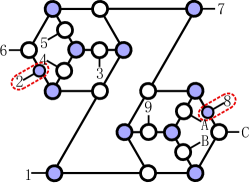
Figure 5: An $N^{4}$MHV example with two auxiliary lines

Then we get the top-form of the on-shell diagram in Fig. 5 after taking the soft limit of line-2

$$\frac{1}{(13456)(1346C)(136BC)(13ABC)(146BC)(19ABC)}$$ (16)

$$\times \frac{1}{(34567)(34579)(4578C)(5678A)(79ABC)(89ABC)}$$

$$\times \frac{(134BC)(379AC)^{2}(5678C)^{2}(567AC)^{3}}{(579AC)(3578C)^{2}(5679A)^{2}(678AC)^{2}}.$$

The geometry constraints are

$$(3,4,5,6)^{2},\ (9,A,B)^{2},\ (8,A,B,C)^{3},\$$

$$(B,C,1,4,6)^{4},\ (1,5,6,7,9)^{4}.$$ (17)

We then take the soft-limit of line-8. We use the gauge $GL(k+1)/GL(k)$ to set the $C^{\prime}$ as

$$\bordermatrix{&1&3&4&5&6&7&8&9&A&B&C\cr&*&*&*&*&*&*&0&*&*&*&*\cr&*&*&*&*&*&*&0&*&*&*&*\cr&*&*&*&*&*&*&0&*&*&*&*\cr&*&*&*&*&*&*&0&*&*&*&*\cr&c_{1}&c_{3}&0&0&c_{6}&0&1&0&c_{A}&c_{B}&c_{C}\cr}.$$

Here we choose $c_{4}=c_{5}=c_{7}=c_{9}=0$. Using the constraints $(3,4,5)^{2},\ (4,5,6)^{2}$, $(9,A,B)^{2},\ (B,C,1,4,6)^{4},$ $\ (1,5,6,7,9)^{4}$, we can find the poles at $c_{3}\rightarrow 0,\ c_{6}\rightarrow 0,\ c_{1}\rightarrow 0,\ c_{A}\rightarrow\frac{(9Ax_{1}x_{2})}{(9Bx_{1}x_{2})}c_{B},\ c_{C}\rightarrow\frac{(146C)}{(146B)}c_{B}$, which are shown in the integrand as

$$(13456) = (3456)c_{1},$$

$$(34567) = -(3457)c_{6},$$

$$(34579) = (4579)c_{3},$$

$$(136BC) = (136B)(c_{C}-\frac{(136C)}{136B}c_{B}),$$

$$(79ABC) = (79BC)(c_{A}+(\frac{(146C)(79AB)}{(146B)(79BC)}-\frac{(79AC)}{(79BC)})c_{B}).$$

Similar as the soft limit of line-2, the other minors are reduced as

$$(3578C) = -(357C),(4578C)=-(457C),$$

$$(678AC) = (67AC),(89ABC)=(9ABC),$$

$$(5678A) = -(567A),(5678C)=-(567C),$$

$${(134BC)\over(146BC)} = {(134B)\over(146B)},$$

$$(1346C) = \frac{(1346)(146C)}{(146B)}c_{B},$$

$$(5679A) = \frac{(5679)(9A13)}{(9B13)}c_{B},$$

$$(13ABC) = -\frac{(1369)(13AB)(13BC)}{(139B)(136B)}c_{B},$$

$$(19ABC) = -\frac{(1469)(14BC)(19AB)}{(146B)(149B)}c_{B},$$

$$(579AC) = -\frac{(579A)(1469)(14BC)}{(149B)(146B)}c_{B},$$

$$(379AC) = -\frac{(379A)(1469)(46BC)}{(469B)(146B)}c_{B},$$

$$(567AC) = \left({(567A)(146C)\over(146B)}-{(567C)(9A13)\over(9B13)}\right)c_{B}.$$

Then we get the integrand of the original on-shell diagram without auxiliary lines

$$\frac{1}{(1346)(1369)(3456)(3457)(4579)(5679)(579A)}$$

$$\times \frac{(134B)}{(146C)(37AB)(13BC)(19AB)(79BC)(9ABC)}$$

$$\times \frac{((367C)(379A)(146B)-(567A)(146C)(379B))^{3}}{(146B)^{3}(67AC)^{2}(357C)^{2}},$$

with the geometry constraints $(3,4,5,6)^{2},(9,A,B,C)^{2}$.

7 Summary and Outlook

We have obtained the top-form integrands for nonplanar leading singularities by BCFW decompositions. In the cases that one cannot attach a BCFW-bridge we add an auxiliary external momentum line judiciously to enable the application of the chain of BCFW decompositions and take the soft limit on the auxiliary momentum line to recover the original diagrams. This combination of strategies is efficient on computing the leading singularity of nonplanar diagrams of arbitrary loops. We have also classified nonplanar on-shell diagrams according to whether they possess rational top-forms, and proved its equivalence to linear BCFW bridges (and rational soft limit for diagrams with no external BCFW bridges). With the chain of BCFW-bridge decompositions obtained the rational top-forms of the nonplanar on-shell diagrams can be derived in a straightforward way. This method applies to leading singularities of nonplanar multi-loop amplitudes beyond MHV.

An immediate question is whether all on-shell diagrams representing nonplanar leading singularities belong to this class, so that all leading singularities can be expressed in the rational top-forms.

Top-form, being simple and compact, is a usefull tool to uncover hidden symmetries (e.g. generalized Yangian symmetry beyond planarity du2014permutation ) which are otherwise highly tangled in nonplanar leading singularities. When combined with the generalized unitarity cuts, top-form holds promise in constructing the integrals as well as revealing the symmetries and dualities of loop-level scattering amplitudes.

Mathematically our method of performing the BCFW decompositions is related to the toric geometry arising in the characterization of Matroid Stratification. Further exploration on the relationship between BCFW decompositions and Matroid Stratification will also shed light on the geometry of underlying Grassmannian manifolds.

8 Acknowledgments

G. Chen thanks Nima Arkani-Hamed, Tianheng Wang for helpful discussion and useful comments. We thank Peizhi Du, Shuyi Li and Hanqing Liu for constructive discussion. Yuan Xin thanks Bo Feng for introducing the background on the recent developments of scattering amplitude. This research project has been supported by the Fundamental Research Funds for the Central Universities under contract 020414340080, the Youth Foundation of China under contract 11405084. This research project has been supported in parts by the NSF China under Contract No. 11775110, No. 1169-0034. We also acknowledge the European Union’s Horizon 2020 Research and Innovation (RISE) programm under the Marie Skĺodowska-Curie grant agreement No.-644121, and the Priority Academic Program Development for Jiangsu Higher Education Institutions (PAPD).

References

- (1) B. Chen, G. Chen, Y. K. E. Cheung, Y. Li, R. Xie and Y. Xin, Eur. Phys. J. C 77 (2017) no.2, 80, arXiv:1411.3889 [hep-th].
- (2) A. Postnikov, “Total positivity, Grassmannians, and networks,” arXiv:math/0609764
- (3) S. Franco, D. Galloni and A. Mariotti, JHEP 1408 (2014) 038, arXiv:1310.3820 [hep-th].
- (4) N. Arkani-Hamed, J. L. Bourjaily, F. Cachazo, A. B. Goncharov, A. Postnikov, et al., (2012), arXiv:1212.5605 [hep-th].
- (5) N. Arkani-Hamed, F. Cachazo, C. Cheung, and J. Kaplan, JHEP 3, 110 (2010), arXiv:0903.2110 [hep-th].
- (6) M. F. Paulos and B. U. W. Schwab, JHEP 1410, 31 (2014), arXiv:1406.7273 [hep-th].
- (7) Y. Bai and S. He, JHEP 1502 065 (2015), arXiv:1408.2459 [hep-th].
- (8) T. Bargheer, Y. t. Huang, F. Loebbert and M. Yamazaki, Phys. Rev. D 91, no. 2, 026004 (2015), arXiv:1407.4449 [hep-th].
- (9) L. Ferro, T. Lukowski and M. Staudacher, Nucl. Phys. B 889 (2014) 192, arXiv:1407.6736 [hep-th].
- (10) S. Franco, D. Galloni, A. Mariotti and J. Trnka, JHEP 1503 (2015) 128, arXiv:1408.3410 [hep-th].
- (11) H. Elvang, Y. t. Huang, C. Keeler, T. Lam, T. M. Olson, S. B. Roland and D. E. Speyer, JHEP 1412 (2014) 181, arXiv:1410.0621 [hep-th].
- (12) N. Arkani-Hamed, J. L. Bourjaily, F. Cachazo and J. Trnka, JHEP 1206 (2012) 125, arXiv:1012.6032 [hep-th].
- (13) N. Beisert, J. Henn, T. McLoughlin and J. Plefka, JHEP 1004 (2010) 085, arXiv:1002.1733 [hep-th].
- (14) J. Broedel, M. de Leeuw, and M. Rosso, JHEP 1406, 170 (2014), arXiv:1403.3670 [hep-th].
- (15) J. Broedel, M. de Leeuw and M. Rosso, JHEP 1411 (2014) 091, arXiv:1406.4024 [hep-th].
- (16) N. Beisert, J. Broedel, and M. Rosso, Journal of Physics A: Mathematical and Theoretical 47, 365402 ( 2014)
- (17) D. Chicherin, S. Derkachov, and R. Kirschner, Nuclear Physics B 881, 467 ( 2014)
- (18) Z. Bern, E. Herrmann, S. Litsey, J. Stankowicz and J. Trnka, JHEP 1506 (2015) 202, arXiv:1412.8584 [hep-th].
- (19) N. Arkani-Hamed, J. L. Bourjaily, F. Cachazo, A. Postnikov and J. Trnka, JHEP 1506 (2015) 179, arXiv:1412.8475 [hep-th].
- (20) S. Franco, D. Galloni, B. Penante and C. Wen, JHEP 1506 (2015) 199, arXiv:1502.02034 [hep-th].
- (21) S. J. Bidder, N. Bjerrum-Bohr, L. J. Dixon, and D. C. Dunbar, Physics Letters B 606, 189 (2005)
- (22) A. Neitzke, Proceedings of the National Academy of Sciences 111, 9717 ( 2014)
- (23) D. Xie and M. Yamazaki, Journal of High Energy Physics 2012, 1 ( 2012)
- (24) Z. Bern, J. Carrasco, H. Johansson, and R. Roiban, Phys.Rev.Lett. 109, 241602 ( 2012), http://arxiv.org/abs/1207.6666 arXiv:1207.6666 [hep-th]
- (25) P. Du, G. Chen, and Y.-K. E. Cheung, Journal of High Energy Physics 2014, 1 ( 2014)
- (26) N. Arkani-Hamed, J. L. Bourjaily, F. Cachazo, and J. Trnka, Phys.Rev.Lett. 113, 261603 ( 2014 b), http://arxiv.org/abs/1410.0354 arXiv:1410.0354 [hep-th]
- (27) S. Franco, D. Galloni, B. Penante, and C. Wen, arXiv preprint arXiv:1502.02034 ( 2015 b)
- (28) H. Johansson, D. A. Kosower, K. J. Larsen, and M. Sogaard, ( 2015), http://arxiv.org/abs/1503.06711 arXiv:1503.06711 [hep-th]
- (29) R. Kleiss and H. Kuijf, Nuclear Physics B 312, 616 ( 1989)
- (30) Z. Bern, L. J. Dixon, D. C. Dunbar and D. A. Kosower, “One loop n point gauge theory amplitudes, unitarity and collinear limits,” Nucl. Phys. B 425, 217 (1994) [hep-ph/9403226].
- (31) M. Bullimore, “Inverse Soft Factors and Grassmannian Residues,” JHEP 1101, 055 (2011) [arXiv:1008.3110 [hep-th]].
- (32) A. Volovich, C. Wen and M. Zlotnikov, “Double Soft Theorems in Gauge and String Theories,” arXiv:1504.05559 [hep-th].
- (33) T. Klose, T. McLoughlin, D. Nandan, J. Plefka and G. Travaglini, JHEP 1507 (2015) 135 doi:10.1007/JHEP07(2015)135 [arXiv:1504.05558 [hep-th]].