TOPO: Improving remote homologue recognition via identifying common protein structure framework

Abstract

(Extended Abstract)

1 Motivation

Protein structure prediction plays an important role in the fields of bioinformatics and biology. Traditional protein structure prediction approaches include template-based modeling (TBM, including homology modeling, and threading), and free modeling (FM). In particular, a threading algorithm takes a query protein sequence as input, recognizes the most likely fold, and finally reports the alignments of the query sequence to structure-known templates as output. The existing threading approaches mainly utilizes the information of protein sequence profile, solvent accessibility, contact probability, etc. The threading strategy has been shown to be successful in structure prediction of a great amount of proteins; however, the existing threading approaches show poorly performance for remote homology proteins. How to improve the fold recognition for remote homology proteins remains a challenge to protein structure prediction.

The sequences of proteins in remote homology generally show relatively weak signal of structure. However, this does not mean that there is no sequence conservation hints for structure. The success of multiple-templates strategy implies the existence of common frameworks, i.e. some regions of proteins are conservative both in the structure and sequence. Such common frameworks should be responsible to the structural stability and then conservative in the evolution.

Based on this we proposed a novel threading approach in three steps. First, for each template, the common structural frameworks shared by its homologous proteins were calculated. Second, unlike in traditional threading methods where the alignment is made against the whole template, we aligned the query protein sequence against a common framework first. This strategy avoids the drawback of the traditional threading approach, i.e. the alignment of variable regions beyond conserved motifs is prone to bringing in error. Third, the final alignments were generated via aligning query sequence against candidate full-length templates in the family. Briefly speaking, we run TreeThreader[2] to build alignments of query against the new template database, and ranked alignments by E-value for model generation. Finally, we generated models by MODELLER based on candidate alignments. The generated models are ranked according to dDFIRE[3] energy function.

2 Methods

For each template with known structure, all of its remote homology proteins are first identified based on structure alignment. Then, a linear programming was designed to identify the common framework shared by these remote homology proteins.

The common framework identification problem can be described as: given a collection of homologous proteins $H=\{s_{1},\ldots,s_{N}\}$ with length $L_{1},\ldots,L_{N}$, the objective is to find $m$ segments with length $n$ with high sequence conservation and structural similarity. As an example, Fig. 1 shows the common frameworks shared by protein 3gxr_A and its homologous proteins.

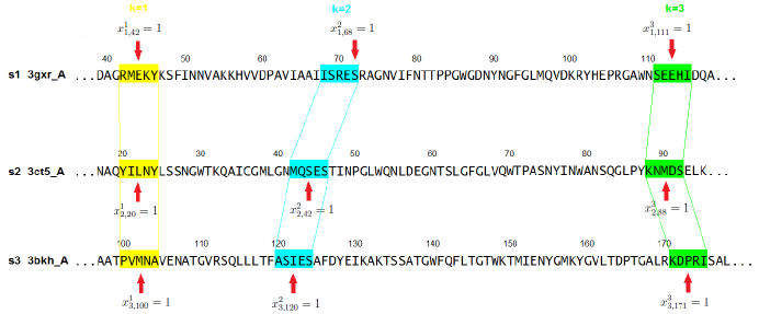
Figure 1: Common frameworks shared by protein 3gxr_A and its homologous proteins. The common framework consists of three dispersed segments (in yellow, cyan, and green). At the conserved segments, the homologous proteins display significant sequence conservation and structural similarity.

2.1 Basic idea of the linear program

The common framework poses double-fold requirements, i.e., significantly high sequence conservation and structural similarity. In the linear program, the objective function was designed to describe structural similarity, and the constraints were designed to describe sequence similarities.

Specifically, the linear program utilizes a set of boolean variables to represent the location of conserved segments, i.e., $x_{ij}^{k}=1$ denotes that in the $i$th protein, the $k$th segment is located at the $j$-th residue. Then, the structural similarity objective and sequence similarity constraints can be described using $x_{ij}^{k}$.

The constraints were designed to represent the following requirements.

• For any sequence, the $k$th segment in common framework is unique;

• No segment in a common framework overlaps nor crosses.

• The segments should have significantly high sequence similarity.

The integer linear programming model can be described as:

$$\ \ \ \ \ \ \ {\rm max}\ \ \ \ \ \ \ \ structural\ similarity\ \ \ \ \ \ \ \ \ \ \ \ \ \ \ \ \ \ \ \ \ \ \ \ \ \ \ \ \ \ \ \ \ \ \ \ \ \ \ \ \ \ \ \ \ \ \ \ \ \ \ \ \ \ \ \ \ \ \ \ \ \ \ \ \ \ \ \ \ \ \ \ \$$

$${\rm s.t.}\ \ \ \ \ \ \ \ \ \ \mathop{\sum}\limits_{j=1}^{L_{i}}x_{ij}^{k} = 1,\ i=1,\ldots,N;k=1,\ldots,m$$ (1)

$$\mathop{\sum}\limits_{j=1}^{C}x_{ij}^{k_{a}}-\mathop{\sum}\limits_{j=1}^{C}x_{ij}^{k_{b}} \geq 0,\ i=1,\ldots,N;C=1,\ldots,L_{i};1\leq k_{a}<k_{b}\leq m$$ (2)

$$x_{ij_{1}}^{k}+x_{ij_{2}}^{k+1} \leq 1,\ i=1,\ldots,N;k=1,\ldots,m-1;1\leq j_{2}<j_{1}+n\leq L_{i}+n$$ (3)

$$M_{i_{1}j_{1},i_{2}j_{2}}*x_{i_{1}j_{1}}^{k}*x_{i_{2}j_{2}}^{k} \geq T,\ i_{1},i_{2}=1,\ldots,N;j_{1}=1,\ldots,L_{i_{1}};j_{2}=1,\ldots,L_{i_{2}};k=1,\ldots,m$$ (4)

where $L_{i}$ denotes the length of the $i$th protein, and $M$ denotes the pre-calculated sequence similarity matrix. In particular, the cell $M_{i_{1}j_{1},i_{2}j_{2}}$ denotes the sequence similarity between of the segment starting from $j_{1}$ in the $i_{1}$th protein and the segment starting from $j_{2}$ in the $i_{2}$th protein.

2.2 Refining the ILP model

In our model, the structure similarity is described using Dscore [1].

$$Dscore(A,B) = \frac{1}{N^{2}}\mathop{\sum}\limits_{i=1}^{L}\mathop{\sum}\limits_{j=1}^{L}\frac{1}{1+(a_{ij}-b_{ij})^{2}}$$

$$\approx \frac{1}{N^{2}}\mathop{\sum}\limits_{i=1}^{L}\mathop{\sum}\limits_{j=1}^{L}(1-(a_{ij}-b_{ij})^{2})$$

where $a_{ij}$ and $b_{ij}$ denote the C_α distance of residue $i$ and residue $j$ in protein $A$ and $B$ respectively.

The final integer linear programming can be formulated as:

$$\ \ \ \ \ \ \ \ \ \ \ \ \ \ \ \ \ \ \ \ \ \ \ \ \ \ \ \ \ \ \ \ \ \ \ \ \ \ \ \ \ {\rm max}\ \ \ \ \mathop{\sum}\limits_{i_{1}=1}^{N}\mathop{\sum}\limits_{i_{2}=1}^{i_{1}}\mathop{\sum}\limits_{j_{11}=1}^{L_{i_{1}}}\mathop{\sum}\limits_{j_{12}=1}^{j_{11}}\mathop{\sum}\limits_{j_{21}=1}^{L_{i_{2}}}\mathop{\sum}\limits_{j_{22}=1}^{j_{21}}\mathop{\sum}\limits_{k_{1}=1}^{m}\mathop{\sum}\limits_{k_{2}=1}^{k_{1}}D_{i_{1}j_{11}j_{12},{i_{2}j_{21}j_{22}}}^{k_{1}k_{2}}*\tau_{i_{1}j_{11}j_{12},{i_{2}j_{21}j_{22}}}^{k_{1}k_{2}}\ \ \ \ \ \ \ \ \ \ \ \ \ \ \ \ \ \ \ \ \ \ \ \ \ \ \ \ \ \ \ \ \ \ \ \ \ \ \$$

$${\rm s.t.}\ \ \ \ \ \ \ \ \ \ \ \ \ \ x_{i_{1}j_{11}}^{k_{1}}+x_{i_{1}j_{12}}^{k_{2}}+x_{i_{2}j_{21}}^{k_{1}}+x_{i_{2}j_{22}}^{k_{2}}-\tau_{i_{1}j_{11}j_{12},{i_{2}j_{21}j_{22}}}^{k_{1}k_{2}} \leq 3$$

$$x_{i_{1}j_{11}^{k_{1}}}-\tau_{i_{1}j_{11}j_{12},{i_{2}j_{21}j_{22}}}^{k_{1}k_{2}} \geq 0$$

$$x_{i_{1}j_{12}^{k_{2}}}-\tau_{i_{1}j_{11}j_{12},{i_{2}j_{21}j_{22}}}^{k_{1}k_{2}} \geq 0$$

$$x_{i_{2}j_{21}^{k_{1}}}-\tau_{i_{1}j_{11}j_{12},{i_{2}j_{21}j_{22}}}^{k_{1}k_{2}} \geq 0$$

$$x_{i_{2}j_{22}^{k_{2}}}-\tau_{i_{1}j_{11}j_{12},{i_{2}j_{21}j_{22}}}^{k_{1}k_{2}} \geq 0$$

$$\mathop{\sum}\limits_{j=1}^{L_{i}}x_{ij}^{k} = 1$$

$$\mathop{\sum}\limits_{j=1}^{C}x_{ij}^{k_{a}}-\mathop{\sum}\limits_{j=1}^{C}x_{ij}^{k_{b}} \geq 0$$

$$x_{ij_{1}}^{k}+x_{ij_{2}}^{k+1} \leq 1$$

$$x_{i_{1}j_{1}}^{k}+x_{i_{2}j_{2}}^{k}-t_{i_{1}j_{1},i_{2}j_{2}}^{k} \leq 1$$

$$x_{i_{1}j_{1}}^{k}-t_{i_{1}j_{1},i_{2}j_{2}}^{k} \geq 0$$

$$x_{i_{2}j_{2}}^{k}-t_{i_{1}j_{1},i_{2}j_{2}}^{k} \geq 0$$

$$M_{i_{1}j_{1},i_{2}j_{2}}-t_{i_{1}j_{1},i_{2}j_{2}}^{k}*T \geq 0$$

where the indicator $\tau_{i_{1}j_{11}j_{12},{i_{2}j_{21}j_{22}}}^{k_{1}k_{2}}$ equals to 1 iff all the four item $x_{i_{1}j_{11}^{k_{1}}}$, $x_{i_{1}j_{12}^{k_{2}}}$, $x_{i_{2}j_{21}^{k_{1}}}$, $x_{i_{2}j_{22}^{k_{2}}}$ equal to 1, and 0 otherwise. The indicator $t_{i_{1}j_{1},i_{2}j_{2}}^{k}$ equals to 1 iff both $x_{i_{1}j_{1}}^{k}$ and $x_{i_{2}j_{2}}^{k}$ equal to 1. The $D$ and $M$ matrix are calculated in advance. The cell $D_{i_{1}j_{11}j_{12},{i_{2}j_{21}j_{22}}}^{k_{1}k_{2}}$ denotes the approximated Dscore of segments start from $j_{11}$ and $j_{21}$ in the $i_{1}$th protein and segments start from $j_{21}$ and $j_{22}$ in the $i_{2}$th protein.

2.3 An example

Fig. 2 shows the common frameworks shared by two domains in SCOP family c.37.1.11. The common frameworks has a Dscore of 8.35 and an RMSD of 1.9Å, implying a significantly high structure conservation.

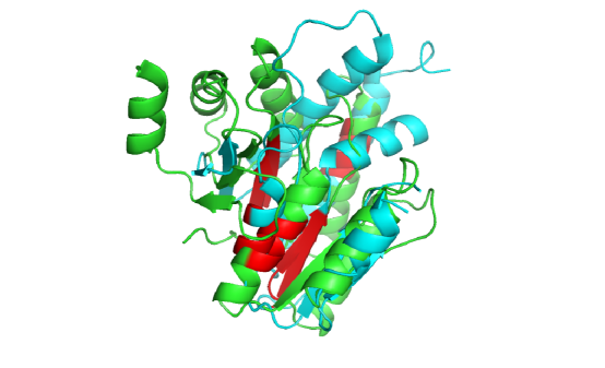
Figure 2: Common frameworks shared by two domains in SCOP family c.37.1.11.

3 Experiments before CASP11

For a total of over 27,000 proteins in PDB70, updated at Apr. 19, 2014, the common frameworks were identified to yield a database called TOPO. The test set consists of 142 pairs of protein structures similar in structure but with low sequence identity. Traditional threading approaches, say HHpred, fail to build an accurate alignment between such protein pairs. In contrast, our alignment method successfully build accruate alignment (TMscore$>0.4$) for seven protein pairs, and generate accurate contact information for 45 protein pairs. Take a pair of protein 3dz1_A vs. 1twd_A as an example. The two proteins share similar protein structure (TMscore=0.56); however, the alignment generated by HHpred has a TMscore of only 0.22. In contrast, our alignment method generates an alignment with TMscore=0.43.

4 Conclusions

Unlike close homology proteins, remote homology proteins show weakly overall sequence signals of structure similarity. However, they still share common frameworks which carry strong sequence signals of structure similarity. Aligning against the common frameworks instead of whole protein sequences improves the fold recognition.

References

- [1] Zhang J, Xu D. Fast algorithm for population‐based protein structural model analysis[J]. Proteomics, 2013, 13(2): 221-229.
- [2] Wu W, Chen G, Kan W, et al. Harness public computing resources for protein structure prediction computing[C]. The International Symposium on Grids and Clouds (ISGC). 2013, 2013.
- [3] Yang Y, Zhou Y. Specific interactions for ab initio folding of protein terminal regions with secondary structures[J]. Proteins: Structure, Function, and Bioinformatics, 2008, 72(2): 793-803.