Facilitation of polymer looping and giant polymer diffusivity in crowded solutions of active particles

Abstract

We study the dynamics of polymer chains in a bath of self-propelled particles (SPP) by extensive Langevin dynamics simulations in a two dimensional system. Specifically, we analyse the polymer looping properties versus the SPP activity and investigate how the presence of the active particles alters the chain conformational statistics. We find that SPPs tend to extend flexible polymer chains while they rather compactify stiffer semiflexible polymers, in agreement with previous results. Here we show that larger activities of SPPs yield a higher effective temperature of the bath and thus facilitate looping kinetics of a passive polymer chain. We explicitly compute the looping probability and looping time in a wide range of the model parameters. We also analyse the motion of a monomeric tracer particle and the polymer’s centre of mass in the presence of the active particles in terms of the time averaged mean squared displacement, revealing a giant diffusivity enhancement for the polymer chain via SPP pooling. Our results are applicable to rationalising the dimensions and looping kinetics of biopolymers at constantly fluctuating and often actively driven conditions inside biological cells or suspensions of active colloidal particles or bacteria cells.

1 Introduction

Active motion is a necessary prerequisite for living systems to maintain vital processes, including materials transport inside cells and the foraging dynamics of mobile organisms [1, 2]. The length scales associated with active motion processes span several orders of magnitude and range from the nanoscopic motion of cellular molecular motors [3] essential to move larger cargo in the crowded environment of cells [4], over the microscopic motion of bacteria cells and micro-swimmers [5, 6], to the macroscopic motion patterns of higher animals and humans [7]. In particular, artificial Janus colloids are propelled by diffusiophoretic or thermophoretic forces [8, 9, 10]. Active motion enhances the speed and precision of signalling and cargo transport in biological cells [11] and allows efficient search of sparse targets for large organisms [12].

A somewhat different question is how passive particles are influenced by an active environment. Tracking the motion of tracer particles immersed in baths of active bacteria [13, 14] and swimming eukaryotic cells [15] one typically observes an enhanced effective tracer mobility, and the active environment may lead to exponential tails of the displacement distribution [15, 16]. Passive particles may also become enslaved to the motion of motor-cargo complexes due to cytoplasmic drag [17]. When micron sized colloids are immersed in baths with smaller particles, short ranged attractive depletion forces of entropic origin are observed [18]. However, the same colloids in a bath of self-propelled particles (SPPs) may experience long ranged attractive or repulsive forces depending on the SPP characteristics [19]. By tuning the concentration of SPPs the forces between two plates can be controlled [20].

Here we want to focus on the properties of polymer chains in an active liquid. It is known that when a polymer chain is immersed into an SPP bath its extension changes non-monotonically with the activity $F_{a}$ of active particles due to competing effects of active forces and chain elasticity [21, 22]. We study here the extent to which the activity of SPPs alters the internal motion of a polymer chain, specifically, how its end loop formation kinetics becomes affected. Polymer looping or reactions of the chain ends is a fundamental process governing numerous biological functions [23, 24]. Protein mediated DNA looping, for instance, is involved in gene regulatory processes [25, 26, 27], or DNA and RNA constructs may be used as molecular beacon sensors [28].

We quantify the behaviour of a polymer chain immersed in a bath of SPPs in two dimensions, see the snapshot of our systems in figure 1. We find that the activity $F_{a}$ of SPPs differently affects the chain conformations depending on the chain bending stiffness $\kappa$. Concurrently, SPPs significantly enhance the looping kinetics as well as give rise to a giant diffusivity of the centre of mass motion of the chain due to SPP pooling in typical parachute like chain configurations. We analyse the diffusion of a monomeric tracer particle, which shows superdiffusive motion on short time scales and Brownian behaviour with enhanced diffusivity in the long time limit. In references [21, 22] a similar system was considered, the main focus being on equilibrium polymer properties such as the gyration radius of the chain. Below we systematically analyse dynamic properties of the polymer chain. Our results demonstrate that the equilibrium and dynamic properties of polymers in an SPP bath are to be considered on the same footing.

This paper is organised as follows. We introduce our model and the simulations methods in section 2. In section 3.1 we examine the equilibrium properties of the polymer chain. Section 3.2 presents the main results regarding the polymer looping properties. In section 3.3 we study the dynamical effects of SPPs on the tracer diffusion, in order to understand its implications on the enhancement of the polymer looping kinetics. We summarise our results and discuss their possible applications in section 4.

2 Model and Methods

To study the dynamics of a polymer chain immersed in a bath of SPPs, we employ coarse grained computer simulations. The polymer chain is modelled as a bead spring chain consisting of $n$ monomers of diameter $\sigma$, connected by harmonic springs with the potential

$$U_{\mathrm{s}}=\frac{k}{2}\sum_{i=2}^{n}\Big{(}|\mathbf{r}_{i}-\mathbf{r}_{i-1}|-l_{0}\Big{)}^{2}.$$ (1)

Here $k$ is the spring constant and $l_{0}$ is the equilibrium bond length. The self avoidance of the chain monomers is modelled by the repulsive part of the Lennard-Jones (LJ) potential (the so called Weeks-Chandler-Andersen or WCA potential),

$$U_{\mathrm{LJ}}(r)=4\epsilon\left[\left(\frac{\sigma}{r}\right)^{12}-\left(\frac{\sigma}{r}\right)^{6}\right]+C(r_{\mathrm{cut}}).$$ (2)

for $r\leq r_{\mathrm{cut}}$, where $r_{\mathrm{cut}}$ is a cutoff length. Moreover $C(r_{\mathrm{cut}})$ is a constant that ensures that $U_{\mathrm{LJ}}(r)=0$ for separations $r>r_{\mathrm{cut}}$, and $r$ is the inter-monomer distance. The potential strength is denoted by $\epsilon$. With the standard choice $r_{\mathrm{cut}}=2^{1/6}\sigma$ for the cutoff length the potential is purely repulsive. In what follows, we measure the length in units of $\sigma$ and the energy in units of the thermal energy $k_{\mathrm{B}}T,$ where $k_{\mathrm{B}}$ is the Boltzmann constant and $T$ is the absolute temperature. Below we set the model parameters to $\sigma=1$, $l_{0}=1.12$, $k=10^{3}$, and $\epsilon=1$.

The bending energy of the chain is given by

$$U_{b}=\frac{\kappa}{2}\sum_{i=2}^{n-1}\Big{(}\mathbf{r}_{i-1}-2\mathbf{r}_{i}+\mathbf{r}_{i+1}\Big{)}^{2},$$ (3)

where $\kappa$ is the bending stiffness. For a given value of $\kappa$, the chain persistence length is $l_{p}\sim 2\kappa l_{0}^{3}/(k_{\mathrm{B}}T)$ in two dimensions. The end monomers are subject to short ranged attractive interactions with energy $\epsilon_{s}$, mimicking the biologically relevant situation that closed structures are energetically profitable, as known for specific DNA looping [25] or closed single stranded DNA (hairpins) [29]. We include the attractive interactions via the LJ potential in Eq. (2) but with a larger cutoff distance and attraction strength $\epsilon_{s}$, namely

$$U_{\mathrm{att}}(r)=U_{\mathrm{LJ}}(r,\epsilon_{s})$$

and $r_{\mathrm{cut}}=2\sigma$. The effects of the end-to-end stickiness on the looping properties were considered by us recently [30]. In what follows we set $\epsilon_{s}=5k_{\mathrm{B}}T$.

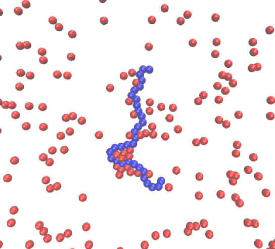
Figure 1: Typical conformation of a polymer (blue chain) in a bath of active particles (red discs) in two dimensions. Parameters: the polymerisation degree of the chain is $n$=32, the packing fraction of SPPs is $\phi$=0.1, and the particle activity is $F_{a}$=40 (see text for details). Video files for different chain lengths and SPP activities are available in the Supplementary Material.

The dynamics of the position $\mathbf{r}_{i}(t)$ of the $i$th chain monomer is described by the Langevin equation

$$m\frac{d^{2}{\mathbf{r}}_{i}(t)}{dt^{2}}=-\boldsymbol{\nabla}[U_{\mathrm{s}}+U_{\mathrm{LJ}}(r)+U_{b}]-\gamma\frac{d\mathbf{r}_{i}}{dt}+\boldsymbol{\xi}_{i}(t).$$ (4)

Here $m$ is the monomer mass, $\gamma$ is its friction coefficient coupled to the diffusivity via

$$D=k_{\mathrm{B}}T/\gamma,$$ (5)

and $\boldsymbol{\xi}_{i}(t)$ represents a Gaussian white noise source of zero mean with autocorrelation $\langle\boldsymbol{\xi}_{i}(t)\cdot\boldsymbol{\xi}_{i^{\prime}}(t^{\prime})\rangle=4\gamma k_{\mathrm{B}}T\delta_{i,i^{\prime}}\delta(t-t^{\prime})$, where $\delta_{i,i^{\prime}}$ is the Kronecker delta symbol.

The SPPs are modelled as disks of diameter $\sigma$ moving under the action of a constant force along a predefined orientation vector

$$\mathbf{n}_{j}=\left\{\cos(\theta_{j}),\sin(\theta_{j})\right\}.$$ (6)

SPPs interact with each other as well as with polymer monomers via the WCA potential (2), and the position of each SPP is governed by the Langevin equation [22]

$$m\frac{d^{2}{\mathbf{r}}_{j}(t)}{dt^{2}}=-\boldsymbol{\nabla}U_{\mathrm{LJ}}(r)+F_{a}\mathbf{n}_{j}(t)-\gamma\frac{d\mathbf{r}_{j}}{dt}+\boldsymbol{\xi}_{j}(t).$$ (7)

Here $F_{a}$ is the active force amplitude, which is directly related to the SPP propulsion strength: it can be expressed in terms of the Péclet number $\mathrm{Pe}$ and the particle velocity $v$ in terms of

$$\mathrm{Pe}=\frac{v\sigma}{D}=\frac{F_{a}\sigma}{k_{\mathrm{B}}T}.$$ (8)

The orientation $\theta_{j}$ of the velocity of the $j$th SPP is changing as function of time according to the standard stochastic equation

$$\dot{\theta}=\sqrt{2D_{r}}\times\xi_{r}(t).$$ (9)

Here $\xi_{r}$ is the Gaussian white noise associated with the rotational diffusivity $D_{r}$ which satisfies the relation $D_{r}=3D/\sigma^{2}$ (see, for instance, reference [22]). Passive particles correspond to $F_{a}=0$, the situation studied in the context of polymer looping with macromolecular crowding in reference [30].

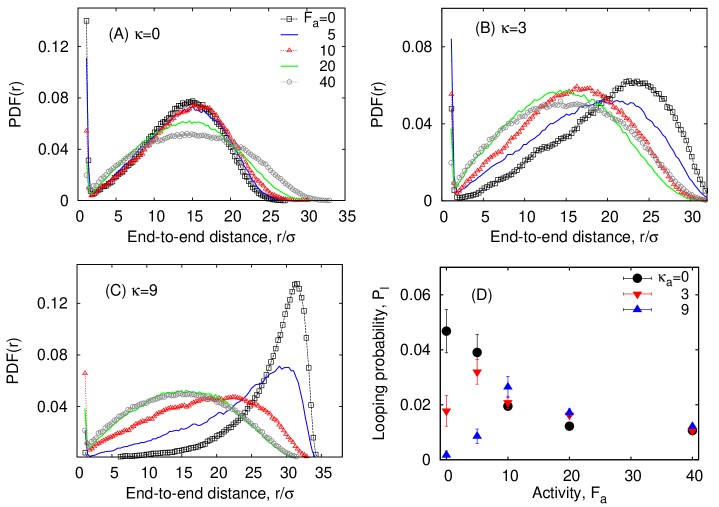
Figure 2: Probability distribution of the polymer end-to-end distance for different SPP activities $F_{a}$ and varying chain bending stiffness: (A) $\kappa=0$, (B) $\kappa=3$, and (C) $\kappa=9$. In (D) the looping probability $P_{l}$ is plotted as function of $F_{a}$ for $n=32$ and $\phi=0.05$.

In our simulations we use periodic boundary conditions for a square box of area $L^{2}$ where, depending on the length of the simulated chain, $L$ varies from 60 to 80. The packing fraction of SPPs is defined as $\phi=N_{\mathrm{cr}}A_{\mathrm{cr}}/L^{2}$, where $N_{\mathrm{cr}}$ is the number of SPPs and $A_{\mathrm{cr}}=\pi(\sigma/2)^{2}$ is the area of a single SPP. We consider rather dilute SPP systems with $\phi\leq 0.1$. For both chain monomers and active particles we choose the unit mass $m=1$ and a relatively large friction of $\gamma=5$ to ensure a quick momentum relaxation. The time scale in the system is set by the elementary time $t_{0}=\sigma\sqrt{m/(k_{\mathrm{B}}T)}$ [31]. We implement the Verlet velocity algorithm [31] to simulate equation (4) and equation (7). The integration time step is $\Delta t=0.002$, and we typically run $\sim 10^{8\ldots 9}$ steps to compute the quantities of interest.

Generally the activity of SPPs may vary, or some particles in the bath may be completely inactive. To account for this fact, in a part of our study below we consider mixtures of active and inactive particles with respective fractions $\phi_{a}$ and $\phi_{i}$. All these particles have the same mass and radius in the simulations.

3 Main Results

3.1 Polymer Dimensions

We first consider the probability distribution function (PDF) of the end to end distance $r$ of the chain as extracted from long time computer simulations, see figure 2A-C. In our simulations, due to the attraction between the end monomers the standard PDF of the polymer [27] acquires an additional peak around the minimum of the attraction potential at the end to end distance $r\sim 2^{1/6}\sigma$. For a flexible chain with $\kappa=0$ (figure 2A) the chain gets more extended and the peak of the PDF shifts to larger distances when the activity $F_{a}$ of SPPs increases. Conversely, for semiflexible chains with a finite value of the polymer stiffness $\kappa>0$, the peak is shifted to shorter distances (figure 2B,C). These trends are similar to those of reference [19].

This is the main effect of active particles on the static properties of passive polymer chains in solutions. Inspecting snapshots of the simulations (see also figure 1) or the video files in the Supplementary Material, one recognises that active particles effect U or parachute like shapes of the polymer. Such parachute shapes are also observed for membranous red blood cells in cylindrical capillary flows and in blood vessels, see, e.g., reference [32]. For larger $F_{a}$ values, when the SPP forces are much larger than the energetic scale for polymer bending, the PDF of the polymer end to end distance is nearly independent on the chain stiffness $\kappa$.

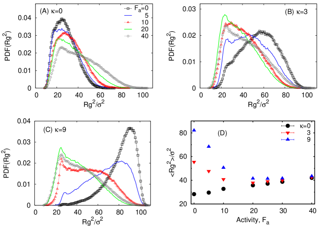
Figure 3: Distribution of the gyration radius for varying $F_{a}$ (in each panel) and bending stiffness (A) $\kappa=0$, (B) $\kappa=3$, and (C) $\kappa=9$. (D) Average gyration radius as function of the SPP activity. Parameters: $n=32$ and $\phi=0.05.$

In figure 3 we also show the distribution of the radius of gyration $R_{g}^{2}$ of the chain and its average value $\left<R_{g}^{2}\right>$. For flexible chains the PDF of the gyration radius broadens towards larger values, causing the monotonic increase of $\left<R_{g}^{2}\right>$. In contrast, for semiflexible chains the gyration radius decreases for $F_{a}\leq 20$, above this value it only slightly increases, compare figure 3D. This behaviour is consistent with the results of references [21, 22].

3.2 Looping Probability and Looping Time

The polymer end to end distance shows a highly erratic behaviour as function of time (see also the movies in the Supplementary Material for chains of different flexibility). The polymer ends tend to remain at short distances $\sim r_{c}$ due to their attractive energy, while longer end to end distances with $r\sim r_{\mathrm{eq}}$ are favourable entropically at equilibrium. We compute the looping probability $P_{l}$ and the looping time $T_{l}$ from the time series of the polymer end to end distance $r(t)$ generated in simulations. Similar to our recent studies [30, 33] the looping probability $P_{l}$ is defined as the fraction of time during which the end to end distance of the chain is shorter than $r_{c}$. In that sense the critical distance $r_{c}=1.75\sigma$ separates the looped and un-looped states of the polymer, compare figure 2A-C.

Figure 2D shows the looping probability $P_{l}$ as function of the activity $F_{a}$ of the SPPs. For flexible chains the value of $P_{l}$ decreases monotonically with $F_{a}$. Conversely, for semiflexible polymers the looping probability is non-monotonic in $F_{a}$. This observation indicates two competing effects of the active particles: on the one hand SPPs increase the effective chain flexibility resulting in higher $P_{l}$ values. On the other hand, SPPs facilitate the unbinding of end monomers. We observe that, consistent with the shape of the end to end distance PDF at large activity $F_{a}$ of SPPs in figures 2A-C, for large $F_{a}$ the looping probability is almost independent of $\kappa$, as demonstrated by figure 2D.

The polymer looping time $T_{l}$ is defined as the time interval within which the distance $r$ reaches $r_{\mathrm{eq}}$ for the first time and the time it gets shorter than the final distance $r_{f}=1.2\sigma$, details are shown in figure 3 of reference [30]. While the distances $r_{c}$ and $r_{f}$ are mainly determined by the properties of the attractive potential of the end monomers, the value of $r_{\mathrm{eq}}$ strongly varies with the chain length and the SPP activity $F_{a}$. From the PDFs of the end to end distances we first determine $r_{\mathrm{eq}}$ for a given chain length $n\sigma$ and particle activity and then use them to compute the looping time $T_{l}$.

Although the effects of SPPs onto the spatial extension of the immersed polymers were considered previously [21, 22], their dynamic effects—particularly on the polymer end looping reaction—were not addressed in detail. In figure 4 we present the polymer looping times as function of the particle activity $F_{a}$. In free space or for $F_{a}=0$ the looping takes much longer for stiffer chains because of the large bending energy required for a loop formation. As the SPP activity $F_{a}$ increases the polymer looping time decreases, especially for stiff chains: we observe a reduction of $T_{l}$ of more than two orders of magnitude, as evidenced in figure 4. Figure 2 shows that for large $F_{a}$ values the looping probability of flexible and semiflexible chains behaves quite similarly, and figure 4 demonstrates similar trends for the looping times $T_{l}$ of the polymer chains for large SPP activities.

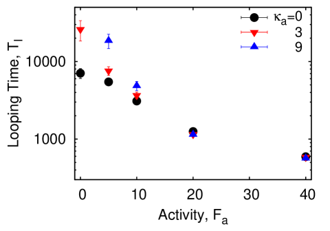
(10)

Figure 4: Polymer looping time versus SPP activity $F_{a}$ for polymer chains with $n$=32 monomers. The simulation time of one point in this figure on a standard workstation is around 6 h. The error bars for $P_{l}$ (figure 2D) and $T_{l}$ were computed as the standard deviation of the mean via subdividing the time traces into ten subsets.

Up to now, we only considered chains of length $n=32$ monomers. In figure 5 we now show the looping times as a function of the chain length $n$. In free space ($\phi=0$), the looping time follows the scaling behaviour [30]

$$T_{l}(n)\sim n^{2\nu+1},$$ (11)

with the Flory exponent $\nu=3/(d+2)=3/4$ for a polymer in two dimensions. With $F_{a}=0$ (inactive crowders) the looping time increases for a given chain length mainly due to a decreasing monomer diffusivity in the medium [30]. In the presence of active crowders the polymer kinetics becomes facilitated, especially for longer chains, as shown by the red dots in figure 5. Interestingly, in the presence of active particles, the scaling exponent of $T_{l}(n)$ decreases somewhat as compared to free space and passive crowders.

Figure 5: Looping time versus chain length, plotted for the situation in free space as well as for conditions of crowded inactive (blue) and active (red symbols) particles. Parameters: $\phi$=0.05 and $\kappa=0$. The asymptotic behaviour of equation (11) is shown as the solid line, the slopes $2.2$ and $2.7$ are also shown.

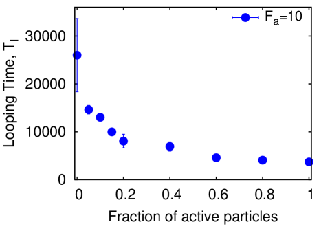
(12)

Figure 6: Polymer looping time versus fraction $\phi_{a}/\phi$ of SPPs at total crowder fraction $\phi$=0.05. The chain length was $n=32$ and the bending stiffness $\kappa=3$.

In figure 6 we show the polymer looping time versus the relative fraction of active particles, $\phi_{a}/\phi$ for the total crowding fraction $\phi=\phi_{a}+\phi_{i}=0.05$. We observe that for small values $\phi_{a}/\phi$ the magnitude of $T_{l}$ initially drops sharply, while the decrease of $T_{l}$ for larger fractions of active particles is rather moderate. This indicates that the transition from the non-active to the active results in figure 5 is rather non-uniform when active particles are added into the solution.

3.3 Tracer Diffusion, Polymer Diffusion and Monomer Displacements

To get a feeling for the effects of SPPs on the diffusion of passive particles we now quantify the enhancement of the diffusive motion of a non-active tracer in a bath of SPPs. We track a particle with diameter $\sigma$ (same size as the monomers and SPPs) for varying SPP activities $F_{a}$. From the time series of the tracer particle position $\mathbf{r}(t)=\{x(t),y(t)\}$ generated in our simulations we calculate the time averaged mean squared displacement (MSD) [34, 35]

$$\overline{\delta^{2}_{x}(\Delta)}=\frac{1}{T-\Delta}\int_{0}^{T-\Delta}\Big{[}x({t^{\prime}+\Delta})-x({t^{\prime}})\Big{]}^{2}dt^{\prime},$$ (13)

where $\Delta$ is the so called lag time defining the width of the averaging window shifted along the trajectory. Hereafter, the time averaged MSD is computed with respect to one dimension only. The additional mean

$$\left<\overline{\delta^{2}(\Delta)}\right>=\frac{1}{N}\sum_{i=1}^{N}\overline{\delta^{2}_{i}(\Delta)}$$ (14)

over an ensemble of $N$ individual traces $\overline{\delta^{2}_{i}(\Delta)}$ will be analysed below.

We present the time averaged MSD of the tracer in figure 7 for varying SPP activity $F_{a}$. The time averaged MSD grows faster than for Brownian motion (superdiffusion [34]) only at very short times, $\Delta^{\star}\lesssim 2\ldots 5$, and then turns into the linear Brownian scaling, as expected. Since the momentum relaxation time, defined as $\sim m/\gamma=0.2$, is shorter than the time scale $\Delta^{\star}$, the extended superdiffusion regime is likely due to the impact of active particles.

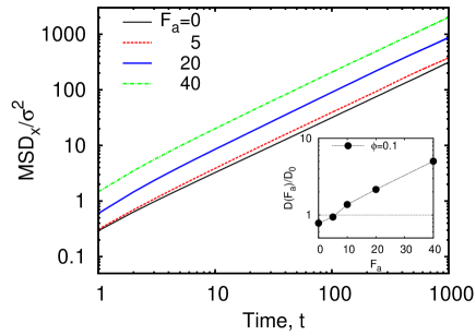
Figure 7: Time averaged MSD $\left<\overline{\delta_{x}^{2}}\right>$ of a single tracer at varying SPP activities $F_{a}$ plotted for $\phi=0.05$. Inset: effective tracer diffusivity, plotted in log-linear scale and normalised to the free space value.

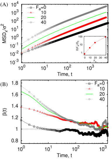
Figure 8: (A) Time averaged MSD of the polymer centre of mass motion, averaged over $N=5$ trajectories, as a function of SPP activity. Inset: Effective diffusivity of the centre of mass motion, normalised to the free-space value. (B) Local scaling exponent $\beta(t)$ of the time averaged MSD. Parameters: $n$=32, $\kappa=0$, and $\phi=0.05.$

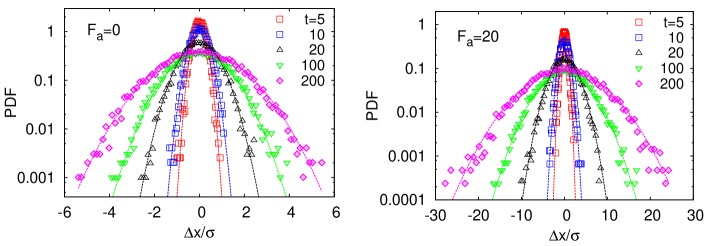
A  B 

Figure 9: PDFs of the centre of mass displacement of the polymer chain (A) and tracer particle (B), plotted for a set of diffusion times $t$ and for two SPP activities at crowding fraction $\phi$=0.05. The dotted lines are Gaussian fits.

We extract the diffusivity of the tracer particle through a linear fit to the long time behaviour of the time averaged MSD in the range $\Delta=10^{2\ldots 3}$. As shown in the inset of figure 7 in log-linear scale the diffusivity increases almost exponentially with $F_{a}$. This enhancement is the main reason of the dramatic facilitation of the polymer looping kinetics by highly active particles, as demonstrated in figure 4 as function of the SPP activity $F_{a}$. This is one of the main conclusions of the current paper.

Similarly, in figure 8A we show the time averaged MSD of the polymer chain’s centre of mass for different SPP activities $F_{a}$. Comparison of the magnitudes of the time averaged MSDs shows that, as expected, the centre of mass diffusion of the entire chain is evidently much slower than that of a single tracer particle. In figure 8B we compute the local scaling exponent of the MSD [34, 35]

$$\beta(\Delta)=\frac{d\log\left<\overline{\delta^{2}(\Delta)}\right>}{d\log(\Delta)}.$$

We observe that at short time scales the MSD increases superdiffusively with $\beta>1$ and the anomalous diffusion exponent grows with increasing $F_{a}$ values. At longer times the diffusion exponent decreases and around $\Delta\simeq 10^{3}$ the motion becomes nearly Brownian, albeit with an enhanced diffusivity at higher $F_{a}$ values.

In the inset of figure 8A we show the chain diffusivity of the centre of mass motion as function of $F_{a}$, normalised with respect to the value in free space. The enhancement of the diffusivity of the polymer centre of mass is nearly two orders of magnitude, that is much higher than that of a monomeric tracer particle shown in the inset of figure 7. This stronger enhancement is due to pooling of SPPs in the concave region of the parachute-shaped polymer chain, resulting in directed motion and faster diffusion of the polymer. This remarkable finding of a giant diffusivity enhancement is our second major result.

We also show the PDFs of the displacement of the polymer chain and of the tracer particle in panels A and B of figure 9, respectively. Both for active and inactive crowders the PDFs exhibit Gaussian profiles, see the dotted fits in the figure. In the presence of active particles, the width of the corresponding displacement PDF becomes wider, consistent with the enhanced diffusivity. This is particularly clear for the polymer centre of mass displacement shown in panel A of figure 9. Interestingly, even at short times—when the time averaged MSD shows a superdiffusive scaling—the PDFs remain nearly Gaussian.

4 Conclusions

Actively driven systems are inherently out of equilibrium and exhibit peculiar behaviours, for instance, in the ratcheting of motors [36], the formation of living crystals [37, 38], phenomena of ordering [39], mesoscale turbulence phenomena [40], or superfluidic behaviour may be observed in bacterial suspensions [41]. Even elementary laws of thermodynamics may no longer hold [42, 43, 44]. In that sense the behaviour of active liquid systems is as rich as that of active soft matter [45].

We studied the dynamics of a polymer chain in a bath of SPPs using Langevin dynamics simulations in two dimensions. We first considered the equilibrium behaviour of the gyration radius, the end to end distance distribution, and the looping probability of the chain as function of the activity of the SPPs. We found that a flexible polymer extends monotonically with the activity. In contrast, for a semiflexible chain—due to a competition of the the chain bending and active forces—the polymer size varies non-monotonically with the particle activity. For a larger activity of SPPs—when active forces become dominant over the chain elasticity effects—the extension of both semiflexible and flexible chains behaves quite similarly.

SPPs also significantly impact the polymer kinetics, the focus of this study. Overall, due to the enhanced diffusivity of the chain monomers, the looping dynamics becomes faster. Especially for the case of stiffer chains the presence of SPPs renders the chains effectively softer, and the looping kinetics is dramatically enhanced in comparison to that of flexible chains. Our results indicate that the activity of a cell medium, as mimicked above by active particles, may indeed facilitate DNA loop formation, effectively making the molecule more flexible.

Examining the motion of a tracer particle in comparison to the motion of the centre of mass of the polymer chain in the bath of SPPs, we observe a giant diffusivity for the driven polymer. We ascribe this to the parachute like shape of the polymer in the SPP bath. Due to the accumulation of SPPs in the concave region of the chain the polymer performs an extended ballistic motion over time scales, that are considerably longer than that of a single monomer. The chain motion at long times becomes Brownian, but with an unexpectedly high diffusivity. Interestingly, even at time ranges on which the time averaged MSD is superdiffusive, the distribution of the particle displacement remains Gaussian. This result differs from experimental observations of an extended exponential decay of the displacement of a tracer in swimming microorganisms [13]. It would thus be interesting to check whether incorporation of hydrodynamic interactions would reproduce such non-Gaussian behaviour in the model of SPP baths. Moreover, it is an interesting questions whether the effect of SPP pooling and the ensuing giant diffusivity enhancement of the polymer motion also arises in three dimensions.

Our analysis here was performed with an in vitro bath of SPPs in mind. In particular the crowding fraction was chosen to be fairly low. Inside living cells active particles such as molecular motors drive the environment out of equilibrium and fluctuating forces inside cells may indeed become an order of magnitude larger than at the conditions of thermal equilibrium [46]. Concurrently, the metabolic cell activity significantly affects the nature of the cytoplasm [47]. However, the (macromolecular) crowding fraction in cells typically is of the order of $30\ldots 35\%$ [48, 49] and thus exceeds the value of our simulations by far. Moreover, these crowders are quite complex macromolecular objects, which tune the reaction kinetics stability of biopolymers [50]. It will therefore be interesting to extend our study to higher crowder fractions and different particle geometries, such as star shapes [51].

References

References

- [1] P. Romanczuk, M. Bär, W. Ebeling, B. Lindner, and L. Schimansky-Geier, Eur. Phys. J. Spec. Topics 202, 1 (2012), and references therein.
- [2] M. C. Marchetti, J. F. Joanny, S. Ramaswamy, T. B. Liverpool, J. Prost, M. Rao, and R. A. Simha, Rev. Mod. Phys. 85, 1143 (2013).
- [3] F. Jülicher, A. Ajdari, and J. Prost, Rev. Mod. Phys. 69, 1269 (1997); A. B. Kolomeisky and M. E. Fisher, Ann. Rev. Phys. Chem. 58 675 (2007); R. D. Astumian and P. Hänggi, Phys. Today 55(11), 33 (2002).
- [4] D. Robert, T. H. Nguyen, F. Gallet, and C. Wilhelm, PLoS ONE 4, e10046 (2010); I. Goychuk, V. O. Kharchenko, and R. Metzler, PLoS ONE 9, e91700 (2014); Phys. Chem. Chem. Phys. 16, 16524 (2014).
- [5] J. Elgeti, R. G. Winkler, and G. Gompper, Rep. Prog. Phys. 78, 056601 (2015), and references therein.
- [6] M. E. Cates, Rep. Prog. Phys. 75, 042601 (2012).
- [7] I. Karamouzas, B. Skinner, and S. J. Guy, Phys. Rev. Lett. 113, 238701 (2014); D. Brockmann, L. Hufnagel, and T. Geisel, Nature, 439, 462 (2006); O. Bénichou, C. Loverdo, M. Moreau and R. Voituriez, Rev. Mod. Phys., 83, 81 (2011); P. C. Bresloff, J. M. Newby, Rev. Mod. Phys. 85, 135 (2013); C. Song, T. Koren, P. Wang, and A.L. Barabási, Nature Physics 6, 818 (2010).
- [8] J. R. Howse, R. A. L. Jones, A. J. Ryan, T. Gough, R. Vafabakhsh, and R. Golestanian, Phys. Rev. Lett. 99, 048102 (2007); W. F. Paxton et al., J. Am. Chem. Soc. 128, 14881 (2006); J. Palacci, C. Cottin-Bizonne, C. Ybert, and L. Bocquet, Phys. Rev. Lett. 105, 088304 (2010);
- [9] H.-R. Jiang, N. Yoshinaga, and M. Sano, Phys. Rev. Lett. 105, 268302 (2010).
- [10] P. Hänggi and F. Marchesoni, Rev. Mod. Phys. 81, 387 (2009); P. K. Ghosh, P. Hänggi, F. Marchesoni, and F. Nori, Phys. Rev. E 89, 062115 (2014).
- [11] C. Loverdo, O. Bénichou, M. Moreau, and R. Voituriez, Nat. Phys. 9, 134 (2008); J. Stat. Mech. P02045 (2009); A. Godec and R. Metzler, Phys. Rev. E 92, 010701(R) (2015); K. Chen, B. Wang, and S. Granick, Nature Mat. 14, 589 (2015).
- [12] G. M. Viswanathan, M. G. E. da Luz, E. P. Raposo, and H. E. Stanley, The Physics of Foraging. An Introduction to Random Searches and Biological Encounters (Cambridge University Press, New York, 2011); M. A. Lomholt, T. Koren, R. Metzler, and J. Klafter, Proc. Natl. Acad. Sci. USA 105, 11055 (2008) V. V. Palyulin, A. V. Chechkin, and R. Metzler, Proc. Natl. Acad. Sci. USA 111 2931 (2014); D. W. Sims et al., Nature 451, 1098 (2008).
- [13] X.-L. Wu and A. Libchaber, Phys. Rev. Lett. 84, 3017 (2000).
- [14] A. Jepson, V. A. Martinez, J. Schwarz-Linek, A. Morozov, and W. C. K. Poon, Phys. Rev. E 88, 041002(R) (2013).
- [15] K. C. Leptos, J. S. Guasto, J. P. Gollub, A. I. Pesci, and R. E. Goldstein, Phys. Rev. Lett. 103, 198103 (2009).
- [16] A. Morozov and D. Marenduzzo, Soft Matter 10, 2748 (2014).
- [17] M. Mussel, K. Zeevy, H. Diamant, and U. Nevo, Biophys. J. 106, 2710 (2014); S. Roy et al, J. Neurosci. 27, 3131 (2007); D. A. Scott et al., Neuron. 70, 441 (2011).
- [18] S. Asakura and F. Oosawa, J. Chem. Phys. 22, 1255 (1954).
- [19] J. Harder, S. A. Mallory, C. Tung, C. Valeriani, and A. Cacciuto, J. Chem. Phys. 141, 194901 (2014).
- [20] R. Ni, M. A. Cohen Stuart, and P. G. Bolhuis, Phys. Rev. Lett. 114, 018302 (2015).
- [21] A. Kaiser and H. Löwen, J. Chem. Phys. 141, 044903 (2014).
- [22] J. Harder, C. Valeriani, and A. Cacciuto, Phys. Rev. E 90, 062312 (2014).
- [23] R. Schleif, Annu. Rev. Biochem. 61, 199 (1992).
- [24] K. S. Matthews, Microbiol. Mol. Biol. Rev. 56, 123 (1992).
- [25] C. Tan, S. Saurabh, M. P. Bruchez, R. Schwartz, and P. LeDuc, Nature Nanotech. 8, 602 (2013); J. M. G. Vilar and I. Saiz, ACS Synth. Biol. 2, 576 (2013).
- [26] B. van den Broek, M. A. Lomholt, S.-M. J. Kalisch, R. Metzler, and G. J. L. Wuite, Proc. Natl. Acad. Sci. U.S.A. 105, 15738 (2008); M. A. Lomholt, B. v. d. Broek, S.-M. J. Kalisch, G. J. L. Wuite, and R. Metzler, Proc. Natl. Acad. Sci. USA 106, 8204 (2009); M. Bauer, E. S. Rasmussen, M. A. Lomholt, and R. Metzler, Sci. Rep. 5, 10072 (2015); D. Swigon, B. D. Coleman, and W. K. Olson, Proc. Natl. Acad. Sci. U.S.A. 103, 9879 (2006); A. Amitai and D. Holcman, Phys. Rev. Lett. 110, 248105 (2013).
- [27] A. G. Cherstvy, Europ. Biophys. J. 40, 69 (2011); A. G. Cherstvy, J. Phys. Chem. B 115, 4286 (2011).
- [28] S. Tyagi and F. R. Kramer, Nat. Biotechnol. 14, 303 (1996); G. Bonnet, O. Krichesvky, and A. Libchaber, Proc. Natl. Acad. Sci. USA 95, 8602 (1998).
- [29] O. Stiehl, K. Weidner-Hertrampf, and M. Weiss, New J. Phys. 15, 113010 (2013).
- [30] J. Shin, A. G. Cherstvy, and R. Metzler, Soft Matter 11, 472 (2015).
- [31] M. P. Allen and D. J. Tildesley, Computer Simulation of Liquids (Clarendon, Oxford, 1994).
- [32] H. Noguchi and G. Gompper, Proc. Natl. Acad. Sci. U. S. A. 102, 14159 (2005).
- [33] J. Shin, A. G. Cherstvy, and R. Metzler, ACS Macro Lett. 4, 202 (2015).
- [34] R. Metzler, J.-H. Jeon, A. G. Cherstvy, and E. Barkai, Phys. Chem. Chem. Phys. 16, 24128 (2014).
- [35] F. Höfling and T. Franosch, Rep. Prog. Phys. 76, 046602 (2013).
- [36] R. Di Leonardo et al., Proc. Natl. Acad. Sci. U. S. A. 107, 9541 (2010).
- [37] J. Palacci, S. Sacanna, A. F. Steinberg, D. J. Pine, and P. M. Chaikin, Science 339, 936 (2013).
- [38] I. Buttinoni, J. Bialke, F. Kuemmel, H. Löwen, C. Bechinger, and T. Speck, Phys. Rev. Lett. 110, 238301 (2013).
- [39] M. Hennes, K. Wolff, and H. Stark, Phys. Rev. Lett. 112, 238104 (2014).
- [40] H. H. Wensink, J. Dunkel, S. Heidenreichd, K. Drescher, R. E. Goldstein, H. Löwen, and J. M. Yeomans, Proc. Natl. Acad. Sci. U. S. A. 109, 14308 (2012).
- [41] H. M. López, J. Gachelin, C. Douarche, H. Auradou, and E. Clément, Phys. Rev. Lett. 115, 028301 (2015).
- [42] S. A. Mallory, A. Saric, C. Valeriani, and A. Cacciuto, Phys. Rev. E 89, 052303 (2014).
- [43] A. P. Solon, Y. Fily, A. Baskaran, M. E. Cates, Y. Kafri, M. Kardar, and J. Tailleur, arXiv: 1412.3952.
- [44] A. P. Solon, J. Stenhammar, R. Wittkowski, M. Kardar, Y. Kafri, M. E. Cates, and J. Tailleur, Phys. Rev. Lett. 114, 198301 (2015).
- [45] A. M. Menzel, Phys. Rep. 554, 1 (2015).
- [46] F. Gallet, D. Arcizet, P. Bohec, and A. Richert, Soft Matter 5, 2947 (2009).
- [47] B. R. Parry, I. V. Surovtsev, M. T. Cabeen, C. S. O’Hern, E. R. Dufresne, and C. Jacobs-Wagner, Cell 156, 183 (2014).
- [48] S. B. Zimmerman and A. P. Minton, Annu. Rev. Biophys. Biomol. Struct. 22, 27 (1993).
- [49] A. R. McGuffee and A. H. Elcock, PLoS Comp. Biol. 6, e1000694 (2010).
- [50] H. Kang, P. A. Pincus, C. Hyeon, and D. Thirumalai, Phys. Rev. Lett. 114, 068303 (2015); H. X. Zhou, G. Rivas, and A. P. Minton, Annual Rev. Biophys. 37, 375 (2008); N. A. Denesyuk and D. Thirumalai, J. Am. Chem. Soc. 133, 11858 (2011); N. M. Toan, D. Marenduzzo, P. R. Cook, and C. Micheletti, Phys. Rev. Lett. 97, 178302 (2006); A. P. Minton, Curr. Opin. Struct. Biol. 10, 34 (2000); M. Yanagisawa, T. Sakaue, and K. Yoshikawa, Intl. Rev. Cell & Molec. Biol. 307, 175 (2014); A. R. Denton, Intl. Rev. Cell & Molec. Biol. 307, 27 (2014).
- [51] J. Shin, A. G. Cherstvy, and R. Metzler, E-print arXiv:1507.01176.