Period-Luminosity Relations Derived From the OGLE-III Fundamental Mode Cepheids II: The Small Magellanic Cloud Cepheids

Abstract

In this paper we present multi-band period-luminosity (P-L) relations for fundamental mode Cepheids in the SMC. The optical $VI$-band mean magnitudes for these SMC Cepheids were taken from the third phase of the Optical Gravitational Lensing Experiment (OGLE-III) catalog. We also matched the OGLE-III SMC Cepheids to 2MASS and SAGE-SMC catalog to derive mean magnitudes in the $JHK$-bands and the four Spitzer IRAC bands, respectively. All photometry was corrected for extinction by adopting the Zaritsky’s extinction map. Cepheids with periods smaller than $\sim 2.5$ days were removed from the sample. In addition to the extinction corrected P-L relations in nine filters from optical to infrared, we also derived the extinction-free Wesenheit function for these Cepheids. We tested the nonlinearity of these SMC P-L relations (except the $8.0\mu\mathrm{m}$-band P-L relation) at 10 days: none of the P-L relations show statistically significant evidence of nonlinearity. When compared to the P-L relations in the LMC, the $t$-test results revealed that there is a difference between the SMC/LMC P-L slopes only in the $V$- and $J$-band. Further, we found excellent agreement between the SMC/LMC Wesenheit P-L slope. The difference in LMC and SMC Period-Wesenheit relation LMC and SMC zero points was found to be $\Delta\mu=0.483\pm 0.015$ mag. This amounts to a difference in distance modulus between the LMC and SMC.

1. Introduction

The period-luminosity relation (the Leavitt Law, hereafter P-L relation) for Small Magellanic Cloud (SMC) Cepheids was first presented in Leavitt & Pickering (1912). Since then, the SMC P-L relations have been derived from optical to near-infrared (for examples, see Arp, 1960; Payne-Gaposchkin, 1965; Wayman, 1984; Welch & Madore, 1984; Visvanathan, 1985; Welch et al., 1985; Caldwell & Coulson, 1986; Laney & Stobie, 1986; Mathewson et al., 1986; Welch et al., 1987; Caldwell & Laney, 1991; Smith et al., 1992; Laney & Stobie, 1994; Nemec, 1994; Sharpee et al., 2002, and references therein) based on relatively small number of SMC Cepheids. In 1999, the second phase of the Optical Gravitational Lensing Experiment (hereafter OGLE-II) released a catalog that contained more than $450$ fundamental mode Cepheids located in $\sim 2.4$ square degree at the center of SMC (Udalski et al., 1999a). A number of SMC P-L relations have been derived in literature based on these OGLE-II SMC Cepheids (Udalski et al., 1999b; Groenewegen, 2000; Storm et al., 2004; Tammann et al., 2008; Sandage et al., 2009; Bono et al., 2010). Independently, the EROS (Expérience de Recherche d’Objets Sombres) Collaboration also derived the P-L relations based on a large number of SMC Cepheids in customized filters (Sasselov et al., 1997; Bauer et al., 1999; Marquette, 1999).

In 2010, a catalog for an even larger number of Cepheids in SMC was released from the the third phase of OGLE operation (hereafter OGLE-III, see Soszyński et al., 2010). Compared to OGLE-II, more than $2600$ fundamental mode SMC Cepheids were included in the OGLE-III SMC catalog as a result of larger survey area (Soszyński et al., 2010). Although the $VI$-band SMC P-L relations were also derived in Soszyński et al. (2010), these P-L relations were not corrected for extinction. Subsequently, Subramanian & Subramaniam (2015) used the OGLE-III $VI$-band photometry for Cepheids to investigate the spatial structure of SMC. In terms of the near infrared $JHK$-band P-L relations, Matsunaga et al. (2011) presented preliminary SMC P-L relations in three period bins by matching the OGLE-III SMC Cepheids to the single-epoch Magellanic Clouds point source catalogs (Kato et al., 2007) based on the Infrared Survey Facility (IRSF) observations. Inno et al. (2013) further combined these IRSF measurements with OGLE-III $VI$-band photometry to derive the period-Wesenheit relations in various combinations. It is expected that more near infrared data for the SMC Cepheids will be available from the VISTA survey of the Magellanic Clouds System Project (VMC Cioni et al., 2011) in the near future.

Using the OGLE-III LMC Cepheid catalog (Soszyński et al., 2008), Ngeow et al. (2009, hereafter Paper I) derived the extinction corrected P-L relations in $VIJHK$ and the four Spitzer IRAC bands. In this work, we extend our investigation and derive the extinction corrected multi-band P-L relations based on the OGLE-III SMC Cepheids using the catalog from Soszyński et al. (2010). It may be noted that the SMC IRAC bands P-L relations were derived in Ngeow & Kanbur (2010) based on single epoch Spitzer data. In this work the IRAC bands P-L relations are updated using the available photometry up to three epochs. The SMC P-L relation is particularly important in distance scale and stellar pulsation work, such as constraining the theoretical predictions (see Bono et al., 2010). This is because the metallicity of SMC is $12+\log(O/H)=7.98$ dex, which is similar or comparable to other local dwarf galaxies (such as IC 1613, 7.86 dex; WLM, 7.74 dex; Sextans A, 7.49 dex; Sextans B, 7.56 dex; Pegasus, 7.92 dex; Leo A, 7.38 dex; see Sakai et al., 2004; Tammann et al., 2011).

2. Data and Extinction Correction

Mean $VI$-band magnitudes and periods for $2626$ fundamental mode SMC Cepheids were taken from Soszyński et al. (2010). The Wesenheit function, $W=I-1.55(V-I)$, was also calculated from the mean $VI$-band magnitudes (if the $V$-band mean magnitude is available). The OGLE-III SMC Cepheids were also matched to the 2MASS point source catalog (Cutri et al., 2003; Skrutskie et al., 2006), using a search radius of $2^{\prime\prime}$. Mean separation of the $2281$ matched 2MASS sources is $0.225^{\prime\prime}$, with a dispersion of $0.264^{\prime\prime}$ (only $60$ matched 2MASS sources have separation greater than $1^{\prime\prime}$). Random-phase corrections as described in Soszyński et al. (2005) were applied to 2MASS photometry to derive the mean $JHK$ magnitudes, using the scaling between $I$-band amplitudes and the $JHK$-band amplitudes. Finally, up to three epochs of the IRAC band photometry, based on publicly released SAGE-SMC (Surveying the Agents of Galaxy Evolution in the Tidally Disrupted, Low-Metallicity Small Magellanic Cloud, Gordon & SAGE-SMC Spitzer Legacy Team, 2010) data, were downloaded from the Spitzer Science Center. As in Paper I and Ngeow & Kanbur (2010), we adopted the SAGE-SMC archival data (version S14 and later, delivered on 2010 September 30) in this work. A search radius of $2^{\prime\prime}$ was used to match the OGLE-III SMC Cepheids and the sources in SAGE-SMC archival data. The number of matched sources and the corresponding mean separations are summarized in Table 1 for the SAGE-SMC Epoch 0, 1 and 2 data. Intensity means were calculated using the three epochs data (when available) for each matched Cepheids in the IRAC bands.

As in Paper I, extinction for each OGLE-III SMC Cepheid was estimated using the Zaritsky et al. (2002) extinction map. For a given input location of SMC Cepheids, this extinction map returns the extinction in $V$-band ($A_{V}$), measured from the cool stars only. In case the extinction maps did not return any extinction values for a given Cepheid, a mean value of $A_{V}=0.18$ was adopted. Extinctions in other bands were scaled using the following total-to-selective extinction coefficient: $R_{V,\ I,\ J,\ H,\ K,\ 3.6\mu\mathrm{m},\ 4.5\mu\mathrm{m},\ 5.8\mu\mathrm{m},\ 8.0\mu\mathrm{m}}=\{3.24,\ 1.96,\ 0.95,\ 0.59,\ 0.39,\ 0.17,\ 0.12,\ 0.08,\ 0.05\}$. Following Paper I, the total-to-selective extinction coefficients in $VI$ bands are adopted from Udalski et al. (1999b), and in other bands these values are calculated based on the extinction law from Cardelli et al. (1989). Our values are slightly different from the value of $R_{V}=3.1$ adopted in Zaritsky et al. (2002) extinction map (Zaritsky, 1999), and almost identical to those used by Fouqué et al. (2007) in $VIJHK$ bands.

3. The Period-Luminosity Relations

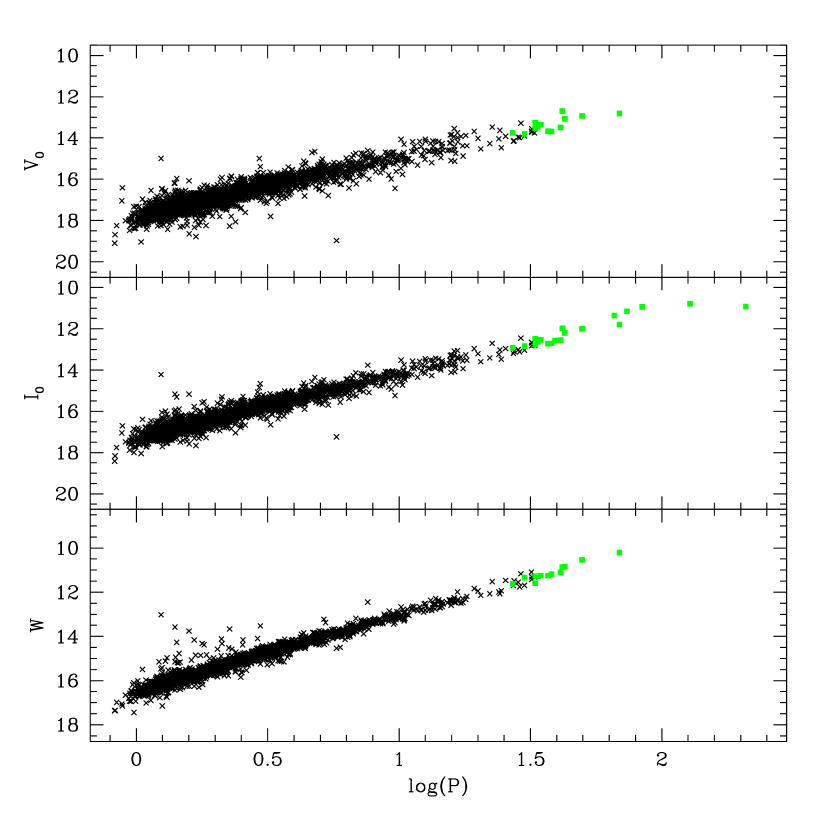
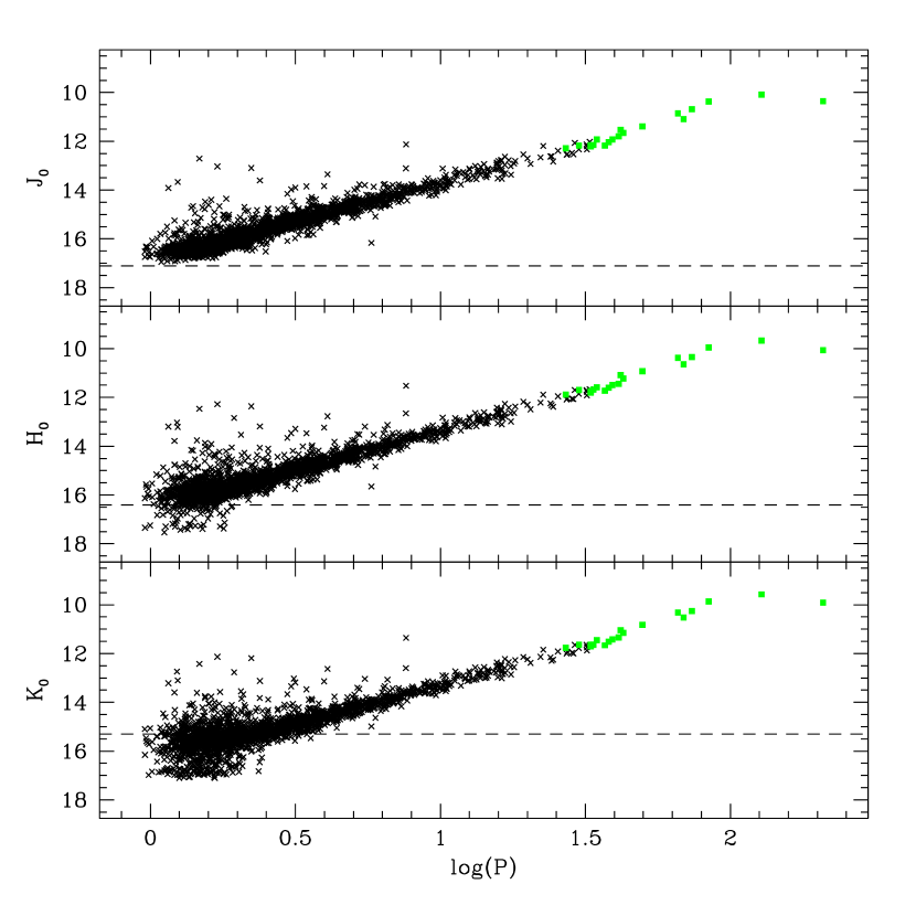
Figure 1.— The extinction corrected SMC P-L relations in $VI$ bands (left panels) and $JHK$ bands (right panels). The extinction-free Wesenheit function is also included in lower-left panel. The (green) filled squares represent the excluded Cepheids at which the OGLE-III photometry was based on the DoPHOT package (see text for more details). The dashed lines in right panels represent the 2MASS $3\sigma$ sensitivity adopted from Cutri et al. (2003).

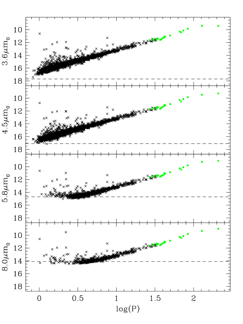
Figure 2.— The extinction corrected SMC P-L relations in IRAC bands for all the matched sources. The (green) filled squares represent the excluded Cepheids at which the OGLE-III photometry was based on the DoPHOT package (see text for more details). The horizontal dashed lines represent the faint limits in each bands, taken from SAGE-SMC document (See http://data.spitzer.caltech.edu/popular/sage-smc/20100930
_enhanced/documents/sage-smc_delivery_sep10.pdf).

Table 1Summary of the Matched SAGE-SMC Archival Data.

Band	$N_{\mathrm{match}}$	$<\Delta>$	Std. Dev.	Fraction within $1^{\prime\prime}$
Epoch 0
$3.6\mu{\mathrm{m}}$	1370	0.314	0.260	97.23%
$4.5\mu{\mathrm{m}}$	1367	0.299	0.254	97.59%
$5.8\mu{\mathrm{m}}$	467	0.287	0.310	95.50%
$8.0\mu{\mathrm{m}}$	361	0.281	0.317	96.12%
Epoch 1
$3.6\mu{\mathrm{m}}$	2580	0.272	0.241	98.22%
$4.5\mu{\mathrm{m}}$	2557	0.271	0.242	98.20%
$5.8\mu{\mathrm{m}}$	702	0.276	0.299	96.30%
$8.0\mu{\mathrm{m}}$	406	0.295	0.313	95.57%
Epoch 2
$3.6\mu{\mathrm{m}}$	2557	0.309	0.242	97.89%
$4.5\mu{\mathrm{m}}$	2545	0.308	0.238	97.92%
$5.8\mu{\mathrm{m}}$	686	0.318	0.277	96.65%
$8.0\mu{\mathrm{m}}$	366	0.334	0.298	95.90%

Extinction corrected mean magnitudes in each band were used to derive the corresponding P-L relations. The resulting P-L relations are presented in Figures 1 and 2. We restricted our Cepheid sample to period range $0.4<\log(P)<1.515$ only. Soszyński et al. (2010) recommended against using the 17 brightest Cepheids listed in the $I$-band catalog for absolute calibration of brightness. The reason is that these Cepheids were not processed with the standard OGLE Difference Image Analysis (DIA) pipeline as these stars saturate in the reference frames. The shortest period of these 17 Cepheids is $\log(P)\sim 1.515$, therefore we adopted an upper limit of the period at $\log(P)=1.515$. Furthermore, Figures 1 and 2 suggest that the slopes of the P-L relations for Cepheids with $\log(P)>1.9$ become flatter in several bands, as they belong to a sub-class of Cepheids – the ultra-long period Cepheids (Bird et al., 2009). The SMC short period Cepheids are known to exhibit a change in the slope of the P-L relation at a specific period. This break period at $\log(P)\sim 0.4$ has been seen in optical data (Bauer et al., 1999; Udalski et al., 1999b; Sharpee et al., 2002; Sandage et al., 2009; Soszyński et al., 2010; Bhardwaj et al., 2014) and extended to mid-infrared (Ngeow & Kanbur, 2010). However, Tammann et al. (2011) suggested the break period might occur at $\log(P)=0.55$, while Subramanian & Subramaniam (2015) found that it could happen at $\log(P)=0.47$. Nevertheless, we adopted $\log(P)=0.4$ as the short period end of our sample. Since our goal is to derive the P-L relations for distance scale applications using the long period Cepheids, detailed investigation into these SMC Cepheids with $\log(P)\leq 0.4$ will be presented elsewhere. Finally, we removed two additional Cepheids (OGLE-SMC-CEP-1157 and OGLE-SMC-CEP-3212), because they were marked in the remarks.txt file as their photometry was derived from the DoPHOT package rather than the DIA method.

$\begin{array}[]{ccc}\includegraphics[angle={0},scale={0.28}]{fig3a.eps}&\includegraphics[angle={0},scale={0.28}]{fig3b.eps}&\includegraphics[angle={0},scale={0.28}]{fig3c.eps}\\ \end{array}$

Figure 3.— The top panels displayed slopes of the fitted P-L relations for data points with $\log(P)>\log(P_{\mathrm{cut}})$ as a function of the adopted period cut. Histograms of the distribution of these fitted P-L slopes were given in the bottom panels. The (red) dashed-lines indicate the mode of the fitted P-L slopes based on the histograms. For $8.0\mu\mathrm{m}$-band P-L slopes, we only derive the mode value from slopes that are smaller than $-3.15$. The vertical arrows represent the adopted $\log(P_{\mathrm{cut}})$ in a given bands. Errors on the P-L slopes are standard errors calculated from the ordinary least squares (OSL) regression method.

Inspecting Figures 1 and 2 suggests that a period cut is needed for $K$-, $5.8$ and $8.0\mu\mathrm{m}$-band P-L relations, after removing $\log(P)\leq 0.4$ Cepheids, to avoid the influence of incompleteness bias at the short-period end. This incompleteness bias is due to the well-known Malmquist bias as discussed, for example, in Sandage (1988). We performed the following steps to determine the appropriate period cuts in the $K$-, $5.8$ and $8.0\mu\mathrm{m}$ bands, respectively.

1. We first adopted an initial period cut at $\log(P_{\mathrm{cut}})=0.4$ and removed Cepheids having periods smaller than this value.

2. We fitted a P-L relation to the remaining sample of Cepheids with an iterative $2.5\sigma$ clipping algorithm to derive the P-L slopes (and its associated error) for this sample of Cepheids.

3. We repeated step 1 and 2 with a binsize in $\Delta\log P=0.01$, up to a maximum value of $\log(P_{\mathrm{cut}})=1.01$. We picked this binsize such that the parameter space of $\log(P_{\mathrm{cut}})$ can be properly sampled. Upper panels of Figure 3 display the fitted P-L slopes as a function of adopted period cuts in $K$, $5.8$ and $8.0\mu\mathrm{m}$ bands.

4. We then plotted the distributions of the P-L slopes given in upper panels of Figure 3 and present these distributions as histograms in the lower panels.

5. Based on these histograms, we determined the mode of the histogram as an indicator that the P-L slopes begin to stabilize (i.e. without the influence of incompleteness at the short period-end) at a given period cut. The values of the mode are shown as horizontal and vertical dashed (red) line in upper and lower panels of Figure 3, respectively.

6. We calculated the absolute deviation between the P-L slopes given in the upper panels of Figure 3 and the modal value determined from the histograms (i.e. the absolute deviation between the horizontal dashed line and individual opened circles in the upper panels of Figure 3).

7. The P-L slope that returned the smallest value of the absolute deviation, based on step 6, is adopted as the final $\log(P_{\mathrm{cut}})$ as indicated by a downward vertical arrow in the upper panels of Figure 3. In case more than one P-L slope resulted in the smallest value of absolute deviation, we adopted the one with minimum value of $\log(P_{\mathrm{cut}})$.

Hence, the final adopted $\log(P_{\mathrm{cut}})$ in $K$-, $5.8\mu\mathrm{m}$- and $8.0\mu\mathrm{m}$-band are $0.51$, $0.68$ and $0.91$, respectively.

Following the OGLE team (Udalski et al., 1999b; Soszyński et al., 2010), obvious outliers of the P-L relations, as displayed in Figures 1 and 2, are removed using an iterative $2.5\sigma$ clipping algorithm (cf. Paper I), where $\sigma$ represents the dispersion of the P-L relation in each iteration. These outliers could be caused by a variety of reasons including, but not limited to, blending of nearby sources, mis-matching of the sources and mis-identification as classical Cepheids in the OGLE-III catalog. For example, Ngeow & Kanbur (2010) discussed the outliers found in the IRAC bands. Since the goal of this work is to derive the P-L relations, we do not investigate the reasons or nature of these outliers in detail. Nevertheless, it is clear that these outliers should be removed in fitting the P-L relations. Figure 4 shows the correlation of residuals of P-L relations in two bands. This demonstrates that the majority of these outliers are present in either or both bands. We have also tried to fit the P-L relations, including the outliers, using the robust regression technique (a regression technique that is robust to outliers presented in the sample, Street et al., 1988; DuMouchel & O’Brien, 1989). The differences obtained in the P-L slopes and zero points using robust regression and our iterative $2.5\sigma$ clipping algorithm do not exceed $0.015$ and $0.012$, respectively, in any given band.

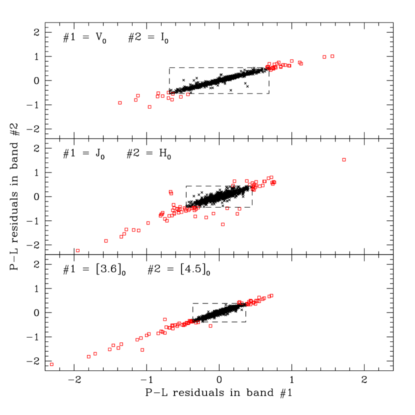
Figure 4.— Correlations of residuals of P-L relations in two bands. Crosses are the Cepheids remained in the sample after applying the iterative $2.5\sigma$ clipping algorithm, while open (red) squares represent the rejected outliers in the P-L relations (in either bands). The dashed boxes represent the $2.5\sigma$ boundaries to reject the outliers, where $\sigma$ is the dispersion of the P-L relation in a given band.

Our final derived P-L relations in various bands for the SMC Cepheids are summarized in Table 2. Slopes of the four IRAC bands and the $VIW$-band P-L relations given in Table 2 are in good agreement with previous determinations as reported in Ngeow & Kanbur (2010), Soszyński et al. (2010) and Subramanian & Subramaniam (2015).

Table 2Multi-Band P-L Relations for SMC Cepheids.

Band	P-L Slope	P-L ZP	P-L Dispersion ($\sigma$)
$V\dots$	$-2.660\pm 0.040$	$17.606\pm 0.028$	0.275
$I\dots$	$-2.918\pm 0.031$	$17.127\pm 0.022$	0.214
$J\dots$	$-3.052\pm 0.026$	$16.773\pm 0.019$	0.182
$H\dots$	$-3.157\pm 0.025$	$16.530\pm 0.018$	0.174
$K\dots$	$-3.213\pm 0.032$	$16.514\pm 0.025$	0.174
$3.6\mu{\mathrm{m}}$	$-3.220\pm 0.021$	$16.433\pm 0.015$	0.146
$4.5\mu{\mathrm{m}}$	$-3.184\pm 0.022$	$16.375\pm 0.016$	0.155
$5.8\mu{\mathrm{m}}$	$-3.201\pm 0.039$	$16.362\pm 0.036$	0.143
$8.0\mu{\mathrm{m}}$	$-3.268\pm 0.087$	$16.426\pm 0.097$	0.156
$W\dots$	$-3.314\pm 0.020$	$16.375\pm 0.014$	0.137

3.1. Comparison with P-L Relations from OGLE-II

Table 3Comparison of SMC P-L Relations.

Ref.	P-L Slope	P-L ZP	$N$	$|T|$	$p$-value
$V$-band
1	$-2.660\pm 0.040$	$17.606\pm 0.028$	912	$\cdots$	$\cdots$
2	$-2.572\pm 0.042$	$17.480\pm 0.032$	466	1.495	0.135
3	$-2.573\pm 0.041$	$17.492\pm 0.032$	464	1.492	0.136
4	$-2.588\pm 0.045$	$17.530\pm 0.035$	460	1.191	0.234
5	$-2.590\pm 0.047$	$17.600\pm 0.019$	488	1.145	0.253
$I$-band
1	$-2.918\pm 0.031$	$17.127\pm 0.022$	918	$\cdots$	$\cdots$
2	$-2.857\pm 0.033$	$17.039\pm 0.025$	488	1.336	0.182
3	$-2.843\pm 0.033$	$17.052\pm 0.025$	487	1.638	0.102
4	$-2.862\pm 0.035$	$17.083\pm 0.027$	462	1.192	0.233
5	$-2.865\pm 0.036$	$17.117\pm 0.014$	488	1.122	0.262
$J$-band
1	$-3.052\pm 0.026$	$16.773\pm 0.019$	883	$\cdots$	$\cdots$
6	$-3.037\pm 0.034$	$16.771\pm 0.027$	418	0.359	0.720
$H$-band
1	$-3.157\pm 0.025$	$16.530\pm 0.018$	875	$\cdots$	$\cdots$
6	$-3.160\pm 0.032$	$16.475\pm 0.025$	414	0.075	0.940
$K$-band
1	$-3.213\pm 0.032$	$16.514\pm 0.025$	627	$\cdots$	$\cdots$
6	$-3.212\pm 0.033$	$16.494\pm 0.026$	418	0.022	0.983
$W$-band
1	$-3.314\pm 0.020$	$16.375\pm 0.014$	909	$\cdots$	$\cdots$
2	$-3.303\pm 0.022$	$16.345\pm 0.017$	469	0.369	0.712
3	$-3.310\pm 0.020$	$16.387\pm 0.016$	463	0.139	0.890
7	$-3.300\pm 0.021$	$16.381\pm 0.016$	446	0.473	0.636

Note. — Reference: (1). this work; (2) Udalski et al. (1999b); (3). same as (2) but updated in ftp://sirius.astrouw.edu.pl/ogle/
ogle2/var_stars/smc/cep/catalog/README.PL; (4) Sandage et al. (2009); (5) Storm et al. (2004); (6) Groenewegen (2000); (7) Groenewegen (2000), with $2.5\sigma$-clipping.

The multi-band P-L relations based on the OGLE-III SMC Cepheids are compared to the P-L relations derived from the OGLE-II catalog in Table 3. As in Paper I, we applied the $t$-test to test the consistency of P-L slopes derived here to the published values. The calculated $T$-values and the corresponding $p$-values (the probability), evaluated based on the $t$-distribution with $\alpha=0.05$ (where $\alpha$ is the adopted significance level), are listed in the last two columns of Table 3. The expected $t$-value from the $t$-distribution, which only depends on $\alpha$ and the degrees of freedom ($\nu$), is $1.968$ for $\nu=300$ or $1.962$ for $\nu=1400$ (which roughly covers the range of $\nu$ in our test). The null hypothesis is that the P-L slopes given in Table 2 are the same as the P-L slopes based on OGLE-II Cepheids. This can be rejected if $|T|>t$, where $t\sim 1.96$ (or equivalently, $p$-value smaller than $0.05$). From Table 3, the P-L slopes in all bands are consistent with those derived from OGLE-II catalogs. We did not consider the updated SMC P-L slopes given in Udalski (2000) as the author assumed the P-L slopes are the same in both LMC and SMC. For $VI$-band P-L relations, we note that different photometric reduction packages were used in OGLE-II (DoPHOT, see Udalski et al., 1998; Udalski, 2000) and OGLE-III (DIA, see Udalski et al., 2008). For common Cepheids with $\log(P)>0.4$ in OGLE-II and OGLE-III catalogs, the averaged difference in mean magnitudes (i.e. OGLE-II minus OGLE-III) is $\sim 0.009$ mag and $\sim 0.004$ mag in $V$- and $I$-band, respectively. After including extinction corrections, the averaged differences increased to $\sim-0.093$ mag in the $V$-band and $\sim-0.057$ mag in the $I$-band. In addition, these differences do not show any dependency on the pulsation period.

4. Testing for Nonlinear P-L Relations at 10 Days

Table 4SMC P-L Relations Separated at 10 Days.

Band	P-L SlopeS	P-L ZPS	$\sigma_{S}$	$N_{S}$	P-L SlopeL	P-L ZPL	$\sigma_{L}$	$N_{L}$
$V\dots$	$-2.634\pm 0.061$	$17.592\pm 0.039$	0.269	821	$-2.453\pm 0.244$	$17.345\pm 0.290$	0.328	91
$I\dots$	$-2.888\pm 0.048$	$17.127\pm 0.022$	0.209	825	$-2.808\pm 0.185$	$16.981\pm 0.220$	0.248	93
$J\dots$	$-3.008\pm 0.041$	$16.748\pm 0.026$	0.180	790	$-2.991\pm 0.144$	$16.684\pm 0.171$	0.195	93
$H\dots$	$-3.114\pm 0.040$	$16.506\pm 0.025$	0.173	781	$-3.149\pm 0.131$	$16.505\pm 0.156$	0.178	94
$K\dots$	$-3.203\pm 0.057$	$16.508\pm 0.040$	0.173	532	$-3.092\pm 0.129$	$16.364\pm 0.153$	0.176	95
$3.6\mu{\mathrm{m}}$	$-3.185\pm 0.034$	$16.413\pm 0.021$	0.146	789	$-3.259\pm 0.112$	$16.468\pm 0.134$	0.152	92
$4.5\mu{\mathrm{m}}$	$-3.166\pm 0.035$	$16.365\pm 0.023$	0.155	797	$-3.108\pm 0.115$	$16.276\pm 0.137$	0.156	93
$5.8\mu{\mathrm{m}}$	$-3.153\pm 0.098$	$16.324\pm 0.080$	0.143	252	$-3.229\pm 0.109$	$16.394\pm 0.130$	0.145	90
$8.0\mu{\mathrm{m}}$	$-2.946\pm 0.909$	$16.121\pm 0.872$	0.146	42	$-3.254\pm 0.121$	$16.409\pm 0.143$	0.161	92
$W\dots$	$-3.320\pm 0.031$	$16.378\pm 0.019$	0.136	817	$-3.274\pm 0.115$	$16.329\pm 0.136$	0.151	92

Note. — The subscripts _S and _L stand for Cepheids with $0.4<\log(P)<1.0$ (i.e. short period Cepheids) and $\log(P)>1.0$ (i.e. long period Cepheids), respectively. $ZP$ and $\sigma$ represents the zero point and dispersion of the P-L relation, respectively. $N$ is the number of Cepheids used in deriving the P-L relations.

The LMC P-L relation is known to exhibit a break at a period around 10 days, as shown in Paper I (and references therein) and Bhardwaj et al. (2015) with rigorous statistical tests. Sandage et al. (2009) proposed that the same break should occur for the SMC P-L relations in optical bands based on an analysis of the period-color relations. However their derived SMC P-L relations do not exhibit a break at 10 days. In the $JHK$-bands, Matsunaga et al. (2011) did not find any significant break at 10 days using the single-epoch data taken from the IRSF. In contrast, studies done in Bono et al. (2010) and García-Varela et al. (2013) suggested that the SMC P-L relations should be nonlinear. In this section we examine the nonlinearity of the SMC P-L relations based on our data presented in previous section, where nonlinearity refers to an underlying P-L relation can be separated to two P-L relations with a break period at 10 days. Table 4 presents the fitted SMC P-L relations for long and short period Cepheids separated at 10 days.

$\begin{array}[]{ccc}\includegraphics[angle={0},scale={0.28}]{fig5a.eps}&\includegraphics[angle={0},scale={0.28}]{fig5b.eps}&\includegraphics[angle={0},scale={0.28}]{fig5c.eps}\\ \end{array}$

Figure 5.— Left Panel: residuals of the fitted P-L relation in Wesenheit function as a function of logarithmic period. Middle Panel: distribution of the residuals presented in the left panel. The fitted Gaussian function to the histogram is shown as dashed (red) curve, with fitted Gaussian parameters $(\mu,\ \sigma)$ given at top of the plot. Right Panel: the $qq$ plot of the residuals. The (red) line represents the case of $y=x$. The theoretical quantiles represent the quantiles if the residuals are drawn from a Gaussian distribution, while the sample quantiles are actual quantiles calculated from the residuals.

As pointed out by Ngeow & Kanbur (2006), statistical tests are needed to find out the nonlinearity of P-L relation. We apply the $F$-test (as in Paper I) and a random walk method in this work to examine the nonlinearity of multi-band SMC P-L relations with a break period at 10 days. The $F$-test requires independent and identically distributed (iid) variables, as well as homoscedasticity and normality of residuals. Since observations of one Cepheid are independent of observations of other Cepheids, the iid assumption is satisfied. We next examine the homoscedasticity assumption (i.e. constant variance) of the P-L residuals. The left panel of Figure 5 displays the residuals of P-L relation: these do not exhibit any obvious trends that violate the homoscedasticity assumption. Further, the average of the P-L residuals are found to be consistent with zero in all bands. Finally, we tested the assumption of normality of the P-L residuals. The middle and right panels of Figure 5 show the histogram and the quantile-quantile ($qq$) plot of the P-L residuals, respectively. The distribution of residuals can be represented with a Gaussian function, as indicated by a dashed curve in middle panel of Figure 5. The $qq$ plot is a common diagnostic tool to evaluate the normality assumption: the quantiles of the data should fall in a diagonal straight line (i.e. the $y=x$ line). Our $qq$ plot demonstrates that the majority of the P-L residuals follow a normal distribution (except few points at the extreme ends of $qq$ plot). Even though in Figure 5 we only showed the results of P-L residuals from the Wesenheit function, P-L residuals in other bands all look very similar to this Figure. Normality of the residuals is important in assuring that the distribution of the $F$-test statistic under the null hypothesis of linearity follows the $F$ distribution. However we can also use a permutation method (as describe below, Kim et al., 2000) to generate the distribution of the $F$ statistic in a way that is independent of the distribution of the residuals.

We fit a single regression line to the actual data and then fit two lines with a break point at a period of 10 days, followed by calculating the $F$-test statistic, $F_{0}$. Details of the $F$-test can be found in Paper I and reference therein, and will not be repeated here. In short, a $F_{0}$ value that is greater than $\sim 3$ would indicate that the underlying P-L relation is nonlinear. If we have $N$ data points we can calculate $N$ residuals from the single straight line fit, ${\epsilon}_{i}$ (where $i=1,\cdots,N$). Next we randomly permute the residuals ${\epsilon}_{i}={\epsilon}_{j}$ and add the permuted residuals back to the fitted data from the single straight line fit. This generates one iteration of pseudo-data. Note the $i^{th}$ data point still has the original period. Now with this pseudo-data, we fit a straight line and then two lines with the original break point and calculate the $F$-test statistic, $F_{1}$. We repeat this process 10,000 times to obtain 10,000 independent $F$-test statistics. We then find the proportion of the $F_{i}$ that are greater than the observed $F_{0}$. This proportion gives the $p$-value, or significance, of the observed $F_{0}$-test statistic without assuming normality. Results of the $F$-test statistic, $F_{0}$ and the $p$-value calculated using the permutation method are summarized in Table 5 for the SMC P-L relations. The largest $F_{0}$-value for the SMC P-L relations is found to be $1.17$ in the $J$-band. Therefore, our $F$-test results strongly suggest that the SMC P-L relations are linear from optical to infrared bands. Our results are further confirmed with a non-parametric random walk test (see Koen et al., 2007; Bhardwaj et al., 2015). A $p(R)$-value from the random walk test such that $p(R)\gtrsim 0.1$ would indicate that the null hypothesis of cannot be rejected. We found that $p(R)>0.3$ in all cases with the exception in the $H$-band P-L relation, which displays a marginal $p$-value (0.06) from the random walk test. We also emphasize that the random walk test is non-parametric and does not make any assumptions about homoscedasticity or normality of residuals. Since the short period Cepheids in $8.0\mu\mathrm{m}$-band only occupied a small period range, $0.91<\log(P)<1.0$, that will cause the determination of the P-L slope to be less accurate ($-2.946\pm 0.909$, see Table 4), we excluded the $8.0\mu\mathrm{m}$-band P-L relation from our statistical tests.

Table 5$F$-test and Permutation Method Results for the Nonlinearity of P-L Relations.

Band	$F_{0}$	$p$
$V\dots$	0.786	0.454
$I\dots$	0.681	0.504
$J\dots$	1.165	0.315
$H\dots$	0.959	0.395
$K\dots$	0.559	0.580
$3.6\mu{\mathrm{m}}$	0.888	0.414
$4.5\mu{\mathrm{m}}$	0.526	0.597
$5.8\mu{\mathrm{m}}$	0.162	0.846
$W\dots$	0.095	0.908

5. Comparison with LMC P-L Relations and the Universal Period-Wesenheit Relation

Table 6Comparison of the P-L slopes Between LMC and SMC Cepheids.

Band	Galaxy	P-L Slope	$|\Delta|$	$|T|$	$p$-value
$V\dots$	SMC	$-2.660\pm 0.040$	$0.109\pm 0.046$	2.558	0.011
	LMC	$-2.769\pm 0.023$
$I\dots$	SMC	$-2.918\pm 0.031$	$0.043\pm 0.034$	1.407	0.160
	LMC	$-2.961\pm 0.015$
$J\dots$	SMC	$-3.052\pm 0.026$	$0.063\pm 0.030$	2.351	0.019
	LMC	$-3.115\pm 0.014$
$H\dots$	SMC	$-3.157\pm 0.025$	$0.049\pm 0.028$	1.930	0.054
	LMC	$-3.206\pm 0.013$
$K\dots$	SMC	$-3.213\pm 0.032$	$0.019\pm 0.035$	0.616	0.538
	LMC	$-3.194\pm 0.015$
$3.6\mu\mathrm{m}$	SMC	$-3.220\pm 0.021$	$0.033\pm 0.023$	1.609	0.108
	LMC	$-3.253\pm 0.010$
$4.5\mu\mathrm{m}$	SMC	$-3.184\pm 0.022$	$0.030\pm 0.024$	1.421	0.155
	LMC	$-3.214\pm 0.010$
$5.8\mu\mathrm{m}$	SMC	$-3.201\pm 0.039$	$0.019\pm 0.044$	0.467	0.641
	LMC	$-3.182\pm 0.020$
$8.0\mu\mathrm{m}$	SMC	$-3.268\pm 0.087$	$0.071\pm 0.094$	0.805	0.421
	LMC	$-3.197\pm 0.036$
$W\dots$	SMC	$-3.314\pm 0.020$	$0.001\pm 0.022$	0.055	0.957
	LMC	$-3.313\pm 0.008$

Since the data sources, algorithms and codes used in this work are almost identical to Paper I, we can compare the P-L slopes found in this work for the SMC Cepheids to the linear version of the LMC P-L slopes given in Paper I. This provides a critical test for the assumption of a universal P-L slopes across different filters. As in the previous section, we applied the statistical $t$-test to test the null hypothesis such that P-L slopes from LMC and SMC Cepheids be the same in a given band. Table 6 summarizes our $t$-test results. We also calculated the (absolute) difference of these P-L slopes, $|\Delta|$, and its associated error ($\sigma_{S}$), which are also provided in Table 6. When comparing the two slopes, it is a common practice in the literature to claim the two underlying slopes as consistent if $\Delta$ is within, say, $\sim 2.5\sigma_{S}$. In this case, the LMC and SMC P-L slopes listed in Table 6 are consistent with each other in all bands. Based on the $t$-test results presented in Table 6, the null hypothesis of equivalent slopes can be rejected for the P-L slopes in $V$- and $J$-band only. The $H$-band P-L slopes, on the other hand, provide evidence of marginal consistency of the slopes. Therefore, the slopes of the P-L relations are not universal in $VJ$ bands, at least for metallicity bracketed by the Magellanic Clouds.

On the other hand, the Wesenheit function, that incorporates a color term, provides evidence of a remarkably consistent P-L slope between the LMC and SMC Cepheids with a value of $\sim-3.31$. This strongly indicates that the Wesenheit function is universal (for example, see discussion in Bono et al., 2010), and hence more suitable for the distance scale application than the single band P-L relations. Since the P-L slopes for Wesenheit function are almost identical, the difference of the P-L zero points for LMC and SMC Wesenheit functions directly translates to the relative distance between LMC and SMC. In terms of distance modulus $\mu$, it is found to be $\Delta\mu=0.483\pm 0.015$ mag, which is in good agreement with the value found in Inno et al. (2013, $\Delta\mu=0.48\pm 0.03$ mag based on fundamental mode Cepheids only) or the preferred value based on Gaussian fitting to a number of recent measurements (Graczyk et al., 2014, $\Delta\mu=0.458\pm 0.068$ mag). The recommended distance moduli for LMC and SMC are $18.49\pm 0.09$ mag (de Grijs et al., 2014) and $18.96\pm 0.02$ mag (de Grijs & Bono, 2015), respectively, with a difference of $\Delta\mu=0.47\pm 0.09$ mag. Again this value is consistent with our result. By shifting the SMC data with $0.483$ mag, we combine the Cepheids in both Magellanic Clouds and derive the following P-L relation for $2578$ Cepheids:

$$W = -3.314(\pm 0.009)\log P+15.892(\pm 0.006),\ \ \sigma=0.099,$$

which, as expected, is identical to the LMC period-Wesenheit relation given in Paper I.

6. Conclusion

The main goal of this study was to extend the work of Paper I by deriving the multi-band P-L relations for SMC fundamental mode Cepheids using the latest compilation of OGLE-III catalog (Soszyński et al., 2010). In addition to the $VI$-band mean magnitudes adopted from Soszyński et al. (2010), we also matched the OGLE-III SMC Cepheids to 2MASS and SAGE-SMC catalogs and derived the mean magnitudes in infrared $JHK$-band and the four IRAC bands. Extinction corrections to these mean magnitudes were done using the Zaritsky et al. (2002) extinction map. These data sources are the same, or very similar, to those adopted in Paper I for the LMC Cepheids. We also applied the almost identical algorithms and codes from Paper I in this work. The difference between this work and Paper I, on the contrary, includes (a) Cepheids with $\log(P)<0.4$ and some longest period Cepheids were excluded in the SMC sample; and (b) we applied a period cut to the $K$, $5.8\mu\mathrm{m}$- and $8.0\mu\mathrm{m}$-band P-L relations to avoid the bias due to incompleteness at the faint end.

We then derived the extinction corrected P-L relations in $VIJHK$ bands and in the four IRAC bands, as well as the extinction free period-Wesenheit function, for SMC fundamental mode Cepheids. Following Paper I, we did not apply absolute calibration to our P-L relation because the readers can adopt their preferred SMC distance to calibrate these P-L relations (for example, the latest measurement of SMC distance can be found in Graczyk et al., 2014). We summarize the main results based on the derived SMC P-L relations as follows:

1. Based on the $F$-test, the SMC P-L relations are found to be linear from optical to infrared bands (except the $8.0\mu\mathrm{m}$-band P-L relation at which the $F$-test is not applied) for SMC Cepheids with period between $\log(P)=0.40$ to $\log(P)=1.51$ (for $K$-band, the period range is $0.51<\log(P)<1.51$; for $5.8\mu\mathrm{m}$ band, the period range is $0.68<\log(P)<1.51$). The period-Wesenheit relation is also linear in the same period range.

2. Based on the $t$-test, the null hypothesis of equivalent slopes for the LMC and SMC P-L relations can be rejected in the $VJ$ bands. The P-L slopes in other bands are consistent between the LMC and SMC Cepheids. We also note the remarkable agreement between the SMC/LMC P-L slopes for the Period-Wesenheit relations.

This work is focused on SMC P-L relations, which are found to be linear as opposed to the nonlinear LMC P-L relations reported in our Paper I (Ngeow et al., 2009) and reference therein. The work of Kanbur et al. (2004), Kanbur & Ngeow (2006) and Kanbur et al. (2007) has provided one possible theoretical scenario by which the LMC P-L relation can be nonlinear whilst the SMC P-L relation is linear. These relate to metallicity differences leading to different mass-luminosity relations obeyed by Cepheids in the Magellanic Clouds and a different hydrogen ionization front-stellar photosphere interaction in terms of periods and phases. The result of identical P-L slopes in LMC and SMC period-Wesenheit relations is interesting, because the $VI$-band P-L slopes for LMC Cepheids are nonlinear but linear in the case of SMC Cepheids. In terms of period-color relation, Kanbur & Ngeow (2004) found that the mean light period-color relations in LMC and SMC are nonlinear and linear, respectively, but Sandage et al. (2009) suggested the SMC period-color relation should be nonlinear. To reconcile the linear and identical slopes in LMC and SMC period-Wesenheit relations implies that the $(V-I)$ period-color relation must play a substantial role here. We will address the issue of period-color relations in a future paper.

Appendix A Correction of $t$-Test Results for LMC Cepheids between OGLE-II and OGLE-III Catalogs in Paper I

Due to a mistake made in the code for performing the $t$-statistical test, the $p$-value was mis-labelled as expected $t$-value based on a $t$-distribution given $\alpha$ and $\nu$. Therefore, the label “t” in Table 2 of Paper I (Ngeow et al., 2009) should be replaced by “$p$-value”, and hence the LMC P-L slopes based on OGLE-II and OGLE-III catalogs are all consistent with each other in all bands. The only exception is the P-L slope for Wesenheit function from Udalski et al. (1999b, c, $-3.277\pm 0.014$ as compared to $-3.313\pm 0.008$ derived in Paper I).

References

- Arp (1960) Arp, H. 1960, AJ, 65, 404
- Bauer et al. (1999) Bauer, F., Afonso, C., Albert, J. N. et al. (EROS Collaboration) 1999, A&A, 348, 175
- Bhardwaj et al. (2014) Bhardwaj, A., Kanbur, S. M., Singh, H. P., & Ngeow, C.-C. 2014, MNRAS, 445, 2655
- Bhardwaj et al. (2015) Bhardwaj, A., Kanbur, S. M., Singh, H. P., Macri, L. M. & Ngeow, C.-C. 2015, MNRAS submitted
- Bird et al. (2009) Bird, J. C., Stanek, K. Z., & Prieto, J. L., 2009, ApJ, 695, 874
- Bono et al. (2010) Bono, G., Caputo, F., Marconi, M., & Musella, I., 2010, ApJ, 715, 277
- Caldwell & Coulson (1986) Caldwell, J. A. R., & Coulson, I. M., 1986, MNRAS, 218, 223
- Caldwell & Laney (1991) Caldwell, J. A. R., & Laney, C. D., 1991, The Magellanic Clouds: Proceedings of the 148th Symposium of the International Astronomical Union. Edited by Raymond Haynes and Douglas Milne. International Astronomical Union. Symposium no. 148, Kluwer Academic Publishers, Dordrecht 148, 249
- Cardelli et al. (1989) Cardelli, J. A., Clayton, G. C., & Mathis, J. S. 1989, ApJ, 345, 245
- Cioni et al. (2011) Cioni, M.-R. L., Clementini, G., Girardi, L., et al. 2011, A&A, 527, AA116
- Cutri et al. (2003) Cutri, R. M., Skrutskie, M. F., van Dyk, S., et al. 2003, The IRSA 2MASS All-Sky Point Source Catalog, NASA/IPAC Infrared Science Archive, VizieR Online Data Catalog, 2246, 0
- de Grijs et al. (2014) de Grijs, R., Wicker, J. E., & Bono, G. 2014, AJ, 147, 122
- de Grijs & Bono (2015) de Grijs, R. & Bono, G. 2015, AJ, 149, 179
- DuMouchel & O’Brien (1989) DuMouchel, W. & O’Brien, F. 1989, Computer Science and Statistics: Proceedings of the 21st Symposium on the Interface. Edited by Kenneth Berk & Linda Malone, American Statistical Association, pg. 297
- Fouqué et al. (2007) Fouqué, P., Arriagada, P., Storm, J., et al. 2007, A&A, 476, 73
- García-Varela et al. (2013) García-Varela, A., Sabogal, B. E., & Ramírez-Tannus, M. C. 2013, MNRAS, 431, 2278
- Gordon & SAGE-SMC Spitzer Legacy Team (2010) Gordon, K. D. & SAGE-SMC Spitzer Legacy Team, 2010, Bulletin of the American Astronomical Society, 41, 489
- Graczyk et al. (2014) Graczyk, D., Pietrzyński, G., Thompson, I. B., et al. 2014, ApJ, 780, 59
- Groenewegen (2000) Groenewegen, M. A. T., 2000, A&A, 363, 901
- Inno et al. (2013) Inno, L., Matsunaga, N., Bono, G., et al. 2013, ApJ, 764, 84
- Kanbur & Ngeow (2004) Kanbur, S. M., & Ngeow, C.-C. 2004, MNRAS, 350, 962
- Kanbur et al. (2004) Kanbur, S. M., Ngeow, C.-C., & Buchler, J. R. 2004, MNRAS, 354, 212
- Kanbur & Ngeow (2006) Kanbur, S. M., & Ngeow, C.-C. 2006, MNRAS, 369, 705
- Kanbur et al. (2007) Kanbur, S. M., Ngeow, C.-C., & Feiden, G. 2007, MNRAS, 380, 819
- Kato et al. (2007) Kato, D., Nagashima, C., Nagayama, T., et al. 2007, PASJ, 59, 615
- Kim et al. (2000) Kim, H.-J., Fay, M. P., Feuer, E. J. & Midthune, D. N. 2000, Statistics in Medicine, 19, 335
- Koen et al. (2007) Koen, C., Kanbur, S., & Ngeow, C. 2007, MNRAS, 380, 1440
- Laney & Stobie (1986) Laney, C. D., & Stobie, R. S., 1986, MNRAS, 222, 449
- Laney & Stobie (1994) Laney, C. D., & Stobie, R. S., 1994, MNRAS, 266, 441
- Leavitt & Pickering (1912) Leavitt, H. S., & Pickering, E. C., 1912, Harvard College Observatory Circular, 173, 1
- Marquette (1999) Marquette, J. B., 1999, New Views of the Magellanic Clouds, 190, 523
- Mathewson et al. (1986) Mathewson, D. S., Ford, V. L., & Visvanathan, N., 1986, ApJ, 301, 664
- Matsunaga et al. (2011) Matsunaga, N., Feast, M. W., & Soszyński, I. 2011, MNRAS, 413, 223
- Nemec (1994) Nemec, J. M., 1994, Stellar and Circumstellar Astrophysics, a 70th birthday celebration for K. H. Bohm and E. Bohm-Vitense. Edited by G. Wallerstein and A. Noriega-Crespo. Astronomical Society of the Pacific Conference Proceedings, 57, 155
- Ngeow & Kanbur (2006) Ngeow, C., & Kanbur, S. M. 2006, ApJ, 650, 180
- Ngeow et al. (2009) Ngeow, C.-C., Kanbur, S. M., Neilson, H. R., Nanthakumar, A., & Buonaccorsi, J., 2009, ApJ, 693, 691 (Paper I)
- Ngeow & Kanbur (2010) Ngeow, C.-C., & Kanbur, S. M., 2010, ApJ, 720, 626
- Payne-Gaposchkin (1965) Payne-Gaposchkin, C., 1965, Veroeffentlichungen der Remeis-Sternwarte zu Bamberg, 27, 178
- Sakai et al. (2004) Sakai, S., Ferrarese, L., Kennicutt, R. C., Jr., & Saha, A. 2004, ApJ, 608, 42
- Sandage (1988) Sandage, A. 1988, PASP, 100, 935
- Sandage et al. (2009) Sandage, A., Tammann, G. A., & Reindl, B., 2009, A&A, 493, 471
- Sasselov et al. (1997) Sasselov, D. D., Beaulieu, J. P., Renault, C., et al. 1997, A&A, 324, 471
- Sharpee et al. (2002) Sharpee, B., Stark, M., Pritzl, B., Smith, H., Silbermann, N., Wilhelm, R., & Walker, A., 2002, AJ, 123, 3216
- Skrutskie et al. (2006) Skrutskie, R. M., Cutri, R. M., Stiening, R., et al., 2006, AJ, 131, 1163
- Smith et al. (1992) Smith, H. A., Silbermann, N. A., Baird, S. R., & Graham, J. A., 1992, AJ, 104, 1430
- Soszyński et al. (2005) Soszyński, I., Gieren, W. & Pietrzyński, G., 2005, PASP, 117, 823
- Soszyński et al. (2008) Soszyński, I., Poleski, R., Udalski, A., et al., 2008, Acta Astronomica, 58, 163
- Soszyński et al. (2010) Soszyński, I., Poleski, R., Udalski, A., et al., 2010, Acta Astronomica, 60, 17
- Storm et al. (2004) Storm, J., Carney, B. W., Gieren, W. P., et al. 2004, A&A, 415, 531
- Street et al. (1988) Street, J. O., Carroll, R. J. & Ruppert, D. 1988, The American Statistician, 42, 152
- Subramanian & Subramaniam (2015) Subramanian, S., & Subramaniam, A. 2015, A&A, 573, AA135
- Tammann et al. (2008) Tammann, G. A., Sandage, A., & Reindl, B. 2008, ApJ, 679, 52
- Tammann et al. (2011) Tammann, G. A., Reindl, B., & Sandage, A. 2011, A&A, 531, AA134
- Udalski et al. (1998) Udalski, A., Szymański, M., Kubiak, M., et al. 1998, Acta Astronomica, 48, 147
- Udalski et al. (1999a) Udalski, A., Soszyński, I., Szymański, M., Kubiak, M., Pietrzyński, G., Woźniak, P., & Zebruń, K., 1999a, Acta Astronomica, 49, 437
- Udalski et al. (1999b) Udalski, A., Szymański, M., Kubiak, M., Pietrzyński, G., Soszyński, I., Woźniak, P., & Zebruń, K. 1999b, Acta Astronomica, 49, 201
- Udalski et al. (1999c) Udalski, A., Soszyński, I., Szymański, M., Kubiak, M., Pietrzyński, G., Woźniak, P., & Zebruń, K. 1999c, Acta Astronomica, 49, 223
- Udalski (2000) Udalski, A. 2000, Acta Astronomica, 50, 279
- Udalski et al. (2008) Udalski, A., Szymański, M. K., Soszyński, I., & Poleski, R. 2008, Acta Astronomica, 58, 69
- Visvanathan (1985) Visvanathan, N., 1985, ApJ, 288, 182
- Wayman (1984) Wayman, P. A. 1984, Irish Astronomical Journal, 16, 188
- Welch & Madore (1984) Welch, D. L., & Madore, B. F., 1984, Structure and Evolution of the Magellanic Clouds, Proceedings of IAU Symposium No. 108. Edited by S. van den Bergh and K. S. D. de Boer. Dordrecht: D. Reidel Publishing Co., 108, 221
- Welch et al. (1985) Welch, D. L., McAlary, C. W., McLaren, R. A., & Madore, B. F., 1985, Cepheids: Theory and Observations, Proceedings of IAU Colloquium No. 82. Edited by B.F. Madore. New York: Cambridge University Press, 82, 219
- Welch et al. (1987) Welch, D. L., McLaren, R. A., Madore, B. F., & McAlary, C. W., 1987, ApJ, 321, 162
- Zaritsky (1999) Zaritsky, D. 1999, AJ, 118, 2824
- Zaritsky et al. (2002) Zaritsky, D., Harris, J., Thompson, I. B., Grebel, E. K., & Massey, P., 2002, AJ, 123, 855