Aspects of Black Holes in Gravitational Theories with Broken Lorentz and Diffeomorphism Symmetries

Abstract

Since Stephen Hawking discovered that black holes emit thermal radiation, black holes have become the theoretical laboratories for testing our ideas on quantum gravity. This dissertation is devoted to the study of singularities, the formation of black holes by gravitational collapse and the global structure of spacetime. All our investigations are in the context of a recently proposed approach to quantum gravity, which breaks Lorentz and diffeomorphism symmetries at very high energies.

B.Sc., M.Sc., M.Phil. Anzhong Wang, Ph.D. Gerald B. Cleaver, Ph.D. Jay R. Dittmann, Ph.D. Truell W. Hyde, Ph.D. Klaus Kirsten, Ph.D. May 2015 J. Larry Lyon, Ph.D. Gregory A. Benesh, Ph.D.

Chapter 1 Introduction

Nature at the most fundamental level is described by four types of interactions, namely the gravitational, electromagnetic, weak and strong interactions. Gravity is best described by the theory of General Relativity, which was proposed in its final form a century ago on November 25, 1915 by Albert Einstein [1]. General Relativity is a classical field theory. The remaining three interactions are all described by quantum field theories. The theory of Quantum Electrodynamics was developed in the late 1940s and early 1950s, largely by Sin-itiro Tomonaga, Julian Schwinger and Richard Feynman [2]. The theory of electro-weak interactions was put together in the 1960s by Sheldon Glashow [3], Steven Weinberg [4] and Abdus Salam [5]. The theory of strong interactions known as Quantum Chromodynamics was discovered in 1973 by David Gross and Frank Wilczek [6], and independently by David Politzer [7]. All these theories are experimentally well tested. But the unsatisfactory fact is that gravity is described by a classical theory while the rest of the fundamental interactions are described by quantum theories, hence the fundamental laws of nature do not constitute one logically consistent system. Despite the fact that this disparity does not affect physics as long as one stays safely below the Planck scale, one is forced into such a high energy regime when studying the very early universe or the final stages of star collapse. This requires a quantum field theory of gravity and perhaps a unification of all the fundamental interactions. The latter goal is pursued by String Theory, while there are quite a few different approaches to quantize gravity.

1.1 Problems of Quantizing Gravity

Soon after Quantum Field Theory was invented and applied to the electromagnetic field by Werner Heisenberg and Wolfgang Pauli [8], it was realized that perturbative computation of the electromagnetic self-energy for an electron led to infinities. Provoked by Pauli, who thought the infinities could be eliminated if gravitational effects were included, Léon Rosenfeld applied Quantum Field Theory to study the gravitational field in 1930 [9]. He showed that the gravitational self-energy of a photon is quadratically divergent in the lowest order of perturbation theory. Later in 1950, using a manifestly gauge-invariant method due to Julian Schwinger, Bryce DeWitt [10] showed that this result implied merely a renormalization of electric charge rather than a non-zero mass of photon and it also implied that the one-loop contribution is zero.

1.1.1 Unitarity

In 1962, while studying the one-loop behavior of General Relativity quantized in a covariant gauge, Richard Feynman noticed that the diagrams are unitary only if fictitious particles are added besides the graviton  [11]. They are fictitious because they were anticommuting bosonic particles circulating in the loop. Such nonphysical fields that are introduced in a manifestly Lorentz covariant quantization procedure to maintain unitarity at one-loop order of perturbation theory are usually referred to as “ghost” fields. DeWitt extended this to the two-loop case in 1964 [12] and to all orders in 1966 [13, 14, 15]. Ghosts were independently introduced by Ludwig D. Faddeev and Victor N. Popov in 1967 [16], who gave a prescription for quantizing Yang-Mills gauge theories in general gauges.

1.1.2 Renormalizability

Even early on, Heisenberg noticed that the gravitational coupling constant $G$ has the dimension of a negative power of mass and consequently the divergences in the perturbation expansion of General Relativity will be different from renormalizable quantum field theories.

In 1974, ’t Hooft and Veltman investigated all the one-loop divergences in General Relativity. They discovered no physically relevant divergences in the one-loop S-matrix. However, the finiteness of pure gravity was destroyed by coupling a single scalar to it [17]. Soon after that, essentially all of the known matter couplings were investigated and it was found that none of the matter fields would share the one-loop finiteness of pure gravity. In 1986, Marc Goroff and Augusto Sagnotti made it clear that our conventional quantization techniques do not work for gravity [18].

Non-renormalizability means simply that the theory is effective and its predictions can be trusted only at sufficiently low energies. For example, the Schrödinger equation is non-renormalizable, yet its predictions are experimentally found to be correct. The same is true for the Four-Fermi Theory of weak interactions. Also, theories that are perturbatively non-renormalizable can be non-perturbatively renormalizable. If there is any hope at all for the renormalizability of General Relativity, that should come from a non-perturbative approach.

1.2 Semi-classical Approach

At the one-loop level, the contribution of the gravitational loop is of the same order as the contributions of matter fields. At usual energies less than the $10^{16}\,$GeV scale, the contributions of additional gravitational loops are highly suppressed. Therefore, a semi-classical concept applies when the quantum matter fields together with the linearized perturbations of the gravitational field interact with the background gravitational field [19, 20, 21].

Not withstanding the difficulties of quantizing gravity, Jacob Bekenstein and Stephen Hawking took up semi-classical studies of black holes in the early 1970’s. In such an approach, the gravitational field is treated as a classical background on which quantum fields are studied. It was shown that black holes behave like black bodies and emit thermal radiation [22, 23]. Hence one can assign temperature and entropy to a black hole. In fact, they showed entropy is proportional to the area of the event horizon [24, 25]. This started the modern era of quantum gravity.

The semi-classical theory of the early universe called Inflationary theory [26] has been very successful too. While black holes are the theoretical laboratories for quantum gravity, Inflation is the experimental laboratory that might give us the first glimpses of quantum gravity [27, 28]. The recent observational constraints [29] on the inflationary gravitational waves imprinted in the cosmic microwave background are strengthening our hopes that experimental quantum gravity is in sight.

1.3 Common Ground

In the absence of experimental data, it is pragmatic to see what common features are shared by different approaches to solve the problems in quantum gravity. Today, reproducing the black hole entropy formula has become a standard test for any theory of quantum gravity. String Theory has successfully reproduced these results, although only in certain extremal black hole cases [30]. In Loop Quantum Gravity, the black hole entropy has been computed for the Schwarzschild black hole, except for a factor of one fourth in the formula, which can be obtained with an appropriate choice of a free parameter of the theory [31]. It is often argued that another common feature shared by theories of quantum gravity is the similar fractal behavior [32]. It is shown that many, if not all, approaches to quantum gravity predict a spectral dimension of 2 in ultraviolet regime. However, it has recently been shown that Bosonic String Theory behaves differently [33]. One has to investigate such a spectral behavior of Superstring Theory before drawing any final conclusions.

1.4 Current Status of Quantum Gravity

To the best of our knowledge today, one cannot have a quantum field theoretic description of General Relativity without an idea from outside the conventional framework. One such idea that has been pursued for many decades is supersymmetry. In 1983, it was established that ${\cal N}=4$ super-Yang-Mills theory in four dimensions is ultraviolet finite to all-loop orders [34]. The supersymmetric version of General Relativity called supergravity showed improved ultraviolet behavior in the early days although it was thought to diverge in the third loop. Now, contrary to all the power-counting arguments, it is shown that ${\cal N}=8$ supergravity in four dimensions is finite to seventh-loop order in perturbation theory [35]. That is a remarkable achievement.

Another area of active research is String Theory whose most fundamental result to date is that under certain caveats, gravity is dual to certain conformal field theories [36]. This result might contain some deeper clues to quantum gravity.

The latest progress comes from a new way of describing gravity within the framework of quantum field theory by breaking Lorentz and diffeomorphism symmetries. This was proposed by Petr Hořava in 2009 [37]. In the relatively short span of its existence, it has been shown that this theory is a part of String Theory and at the same time makes contact with other seemingly different approaches to quantum gravity.

Despite making enormous progress in our understanding of the high energy behavior of gravity, our quest for quantum gravity is far from over.

Chapter 2 Gravitational Theories with Anisotropic Scaling

2.1 Introduction

In the previous chapter, we listed the core problems in quantizing gravity and argued that in order to achieve this feat, we need ideas from outside the conventional framework. The investigations in this dissertation are concerned with the latest of such ideas, inspired by anisotropic scaling in the theories of condensed matter physics. Before diving into the details of gravitational theories with anisotropic scaling, we discuss some important ingredients of the theory and why they are essential.

2.1.1 Higher-order Terms

The non-renormalizability of General Relativity means that it is an effective theory and the Einstein-Hilbert action contains only the terms relevant at low energies. One is naturally tempted to add higher-order curvature terms to the action, thereby making the theory applicable at high energies. This possibility was first explored in 1962 by Ryoyu Utiyama and Bryce S. DeWitt [38]. They noticed that the action of quantum gravity should contain functionals of higher derivatives of the metric tensor besides the Einstein-Hilbert action. But is such a theory renormalizable? This question was answered affirmatively in 1977 by Kellogg Stelle [39]. He showed that the theory is renormalizable with quadratic curvature invariants. However due to the presence of higher time derivatives, such a theory has the negative norm state called “ghosts” which allow the probability to be negative and hence breaks unitarity. In fact, as far back as in 1850, Mikhail Ostrogradsky showed that the presence of time derivatives higher than two generally leads to the problem of ghosts [40]. Combining all these ideas, Hořava added only the terms containing higher spacial derivatives while keeping the time derivatives to the second order. Also, power-counting renormalizability restricts the number of spacial derivatives to at least six. This means that space and time are treated differently and hence the local Lorentz and diffeomorphism symmetries are broken.

2.1.2 Lorentz Invariance

Invariance under the Lorentz symmetry group is a cornerstone of modern physics, and is strongly supported by observations. In fact, all the experiments carried out so far are consistent with it  [41], and no evidence shows that such a symmetry must be broken at certain energy scales, although it is arguable that such constraints in the gravitational sector are much weaker than those in the matter sector  [42]. It should be emphasized that the breaking of Lorentz invariance can have significant effects on low-energy physics through the interactions between gravity and matter, no matter how high the scale of symmetry breaking is [43, 44]. The question of how to prevent the propagation of the Lorentz violations into the Standard Model of particle physics remains challenging [45]. Nevertheless, it is known that demanding renormalizability and unitarity of gravity often lead to the violation of Lorentz invariance [46]. There are benefits of violating Lorentz invariance [47]. Recently, a mechanism of supersymmetry breaking by coupling a Lorentz-invariant supersymmetric matter sector to non-supersymmetric gravitational interactions with Lifshitz scaling was shown to lead to a consistent HL gravity [48].

2.1.3 Diffeomorphism Invariance

In many theories of quantum gravity and especially in String Theory, it is believed that the concept of space and time is an emergent notion that is not present in the fundamental theory [49]. Another way of looking at it is that one does not have to respect the symmetries of spacetime that are thought to be fundamental at known energies, such as the local Lorentz and diffeomorphism symmetries, especially given the fact that our understanding of spacetime at the Planck scale is highly limited.

2.1.4 Ultraviolet Fixed Point

We know from quantum field theory that the value of coupling strengths of fundamental interactions depend on the energy scale at which they are measured. This variation of coupling strengths with energy scale is called the running of the couplings. This has been experimentally seen for the Standard Model interactions. The essential tool for studying this is renormalization group flow, developed by Kenneth G. Wilson [50], which is a sophisticated version of the general theory of thermodynamic phase transitions due to Lev Landau from 1937 [51]. This is closely related to critical phenomena in statistical mechanics [52], originally developed by E. M. Lifshitz in 1941 [53]. A quantum field theory is said to have an ultraviolet fixed point if its renormalization group flow approaches a fixed point at very high energies. Theories with the trivial or Gaussian ultraviolet fixed point are said to be asymptotic free theories. They may be, but not necessarily are, strongly-coupled theories whose study require nonperturbative methods. The famous example is QCD. Hořava-Lifshitz Theory is also thought to be of this kind. Theories with a nontrival or non-Gaussian fixed point are said to be asymptotic safe theories. A notable example is asymptotic safety in quantum gravity proposed by Steven Weinberg [54].

2.2 Hořava-Lifshitz Theory

2.2.1 Original Version

Hořava achieved all the above mentioned objectives in 2009 [37] by borrowing from condensed matter physics the idea of anisotropic scalings [53] of space and time, given by

$${\bf x}\rightarrow\ell{\bf x},\;\;\;t\rightarrow\ell^{z}t,$$ (2.1)

where $z$ is called the dynamical critical exponent. This was first used to construct scalar field theory by E. M. Lifshitz, hence the theory is often referred to as the Hořava-Lifshitz (HL) Theory. The anisotropic scaling provides a crucial mechanism: the gravitational action can be constructed in such a way that only higher-dimensional spatial, but not time, derivative operators are included, so that the UV behavior of the theory is dramatically improved. In $(3+1)$-dimensional spacetimes, HL theory is power-counting renormalizable provided that $z\geq 3$ [37, 55, 56]. In this dissertation, we will assume that $z=3$. At low energies, the theory is expected to flow to $z=1$. In this limit the Lorentz invariance is “accidentally restored.” The exclusion of high-dimensional time derivative operators, on the other hand, prevents the ghost instability, whereby the unitarity of the theory is assured.

The anisotropy between time and space mentioned above is conveniently expressed in terms of the Arnowitt-Deser-Misner (ADM) [57] variables: the lapse function $N$, the shift vector $N^{i}$ and the three-dimensional metric defined on the leaves of constant time $g_{ij}$ where $i,\;j=1,2,3$. In the metric form, it is given by

$$ds^{2} = -N^{2}c^{2}dt^{2}+g_{ij}\left(dx^{i}+N^{i}dt\right)\left(dx^{j}+N^{j}dt\right),~{}~{}~{}~{}~{}~{}~{}~{}(i,\;j=1,2,3).$$ (2.2)

Under the rescaling (2.1) with $z=3$, $N,\;N^{i}$ and $g_{ij}$ scale as

$$N\rightarrow N,\;\;\;N^{i}\rightarrow{\ell}^{-2}N^{i},\;\;\;g_{ij}\rightarrow g_{ij}.$$ (2.3)

The requirement that the foliation defined by these leaves be preserved by any gauge symmetry implies that the theory is covariant only under the action of the group Diff($M,\;{\cal{F}}$) of foliation-preserving diffeomorphisms,

$$\delta{t}=-f(t),\;\;\;\delta{x}^{i}=-\zeta^{i}(t,{\bf x}),$$ (2.4)

for which $N,\;N^{i}$ and $g_{ij}$ transform as

$$\delta{g}_{ij} = \nabla_{i}\zeta_{j}+\nabla_{j}\zeta_{i}+f\dot{g}_{ij},$$

$$\delta{N}_{i} = N_{k}\nabla_{i}\zeta^{k}+\zeta^{k}\nabla_{k}N_{i}+g_{ik}\dot{\zeta}^{k}+\dot{N}_{i}f+N_{i}\dot{f},$$

$$\delta{N} = \zeta^{k}\nabla_{k}N+\dot{N}f+N\dot{f},$$ (2.5)

where $\dot{f}\equiv df/dt$, $\nabla_{i}$ denotes the covariant derivative with respect to the 3-metric $g_{ij}$, and $N_{i}=g_{ik}N^{k}$, etc. From these expressions one can see that the lapse function $N$ and the shift vector $N_{i}$ play the role of gauge fields of the Diff($M,\;{\cal{F}}$) symmetry. Therefore, it is natural to assume that $N$ and $N_{i}$ inherit the same dependence on spacetime as the corresponding generators

$$N=N(t),\;\;\;N_{i}=N_{i}(t,x),$$ (2.6)

which is clearly preserved by Diff($M,\;{\cal{F}}$) and usually referred to as the projectability condition.

The non-projectable version of HL gravity [58] is self-consistent and passes all the solar system, astrophysical and cosmological tests. In fact, in the infrared the theory can be identified with the hypersurface-orthogonal Einstein-aether theory [59] in a particular gauge [60, 61, 62], whereby the consistence of the theory with observations can be deduced.

Problems.

Due to the restricted diffeomorphisms, one more degree of freedom appears in the gravitational sector, i.e., the spin-0 graviton. This is potentially dangerous, and needs to decouple in the infrared in order to be consistent with observations [63]. In particular, the spin-0 mode is not stable in the Minkowski background in the original version of the HL theory  [37] and in the Sotiriou, Visser and Weinfurtner (SVW) generalization [64, 65]. However, in the SVW setup, it is stable in the de Sitter background  [66]. In addition, non-perturbative analysis showed that it indeed decouples in the vacuum spherical static  [67] and cosmological [68] spacetimes.

Another potential complication of the HL theory is that the theory becomes strongly coupled when the energy is very low [69]. However, as long as the theory is consistent with observations when the nonlinear effects are taken into account, this is not necessarily a problem, at least not classically. A careful analysis shows that the theory is consistent with observations in the vacuum spherically symmetry static case [67] and in the cosmological setting [70, 71, 72].

2.2.2 Extended Symmetry

One way to overcome the above problems is to introduce an extra local $U(1)$ symmetry, so that the total symmetry of the theory is extended to  [73]

$$U(1)\ltimes{\mbox{Diff}}(M,\;{\cal{F}}).$$ (2.7)

This is achieved by introducing a gauge field $A$ and a Newtonian prepotential $\varphi$. One consequence of the $U(1)$ symmetry is that the spin-0 gravitons are eliminated [73, 68]. Effectively, the spatial diffeomorphism symmetries of General Relativity are kept intact, but the time reparametrization symmetry is contracted to a local gauge symmetry [74]. The restoration of general covariance, characterized by Eq. (2.7), nicely maintains the special status of time, so that the anisotropic scaling (2.1) with $z>1$ can still be realized. As a result, all problems related to them, such as instability, strong coupling, and different propagation speeds in the gravitational sector, are resolved.

Under the Diff($M,\;{\cal{F}}$), the fields $A$ and $\varphi$ transform as

$$\delta{A} = \zeta^{i}\partial_{i}A+\dot{f}A+f\dot{A},$$

$$\delta\varphi = f\dot{\varphi}+\zeta^{i}\partial_{i}\varphi,$$ (2.8)

while under the local $U(1)$, the gauge fields together with $N$, $N_{i}$ and $g_{ij}$ transform as

$$\delta_{\alpha}A = \dot{\alpha}-N^{i}\nabla_{i}\alpha,$$

$$\delta_{\alpha}\varphi = -\alpha,$$

$$\delta_{\alpha}{N} = 0,$$

$$\delta_{\alpha}N_{i} = N\nabla_{i}\alpha,$$

$$\delta_{\alpha}g_{ij} = 0,$$ (2.9)

where $\alpha$ is the generator of the local $U(1)$ gauge symmetry.

A remarkable by-product of this “non-relativistic general covariant” setup is that it forces the coupling constant $\lambda$, introduced originally to characterize the deviation of the kinetic part of the action from General Relativity [37], to take exactly its relativistic value $\lambda=1$. A different view can be found in [75]. The $U(1)$ symmetry was initially introduced in the case of $\lambda=1$, but the formalism was soon extended to the case of any $\lambda$ [75, 76, 77]. In the presence of a $U(1)$ symmetry, the consistency of the HL theory with solar system tests and cosmology was systematically studied in [78, 79, 80]. In particular, it was shown in [81] that, in order for the theory to be consistent with solar system tests, the gauge field $A$ and the Newtonian prepotential $\varphi$ must be part of the metric in the infrared limit. This ensures that the line element $ds^{2}$ is a scalar not only under ${\mbox{Diff}}(M,\;{\cal{F}})$ but also under the local $U(1)$ symmetry. In this model, the formation of black holes by gravitational collapse was first studied in [82].

Another possibility is to give up the projectability condition (2.6). This allows for new operators to be included in the action, in particular, operators involving $a_{i}\equiv N_{,i}/N$. In this way, all the problems mentioned above can be avoided by properly choosing the coupling constants. However, since this leads to a theory with more than 70 independent coupling constants [83], it makes the predictive power of the theory questionable, although only five coupling constants are relevant in the infrared.

A non-trivial generalization of the enlarged symmetry (2.7) to the nonprojectable, $N=N(t,x)$, case was discovered by Zhu, Wu, Wang and Shu [84, 85]. It was shown that, as in General Relativity, the only degree of freedom of the model in the gravitational sector is the spin-2 massless graviton. Moreover, thanks to the elimination of the spin-0 gravitons, the physically viable range for the coupling constants is considerably enlarged, in comparison with the original non-projectable version, where the extra $U(1)$ symmetry is absent. Furthermore, the number of independent coupling constants is dramatically reduced from more than 70 to 15. The consistency of the model with cosmology was recently established in [85, 86, 87]. In the case with spherical symmetry, the model was shown to be consistent with solar system tests  [88]. In contrast to the projectable case, the consistency can be achieved without taking the gauge field $A$ and Newtonian prepotential $\varphi$ to be part of the metric. Finally, the duality between this version of the HL theory and a non-relativistic quantum field theory was analyzed in [89], and its embedding in String Theory was constructed in [90]. For other examples see [91].

It is remarkable to note that, despite of the stringent observational constraints on the Lorentz violation [41], the non-relativistic general covariant Hořava-Lifshitz gravity constructed in [84] is consistent with all the solar system tests [92, 93] and cosmology  [80, 94].

Table 2.1: A summary of various versions of the Hořava-Lifshitz Theory

Property of the theory	${\mbox{Diff}}(M,{\cal{F}})$			$U(1)\ltimes{\mbox{Diff}}(M,{\cal{F}})$
	$N=N(t)$	$N=N(t,x)$		$N=N(t)$	$N=N(t,x)$
Independent Couplings	11	$>$75		11	15
No Spin-0 Graviton	X	X		$\checkmark$	$\checkmark$
No instability of $M_{4}$	X	$\checkmark$		$\checkmark$	$\checkmark$
No Strong Coupling	X	$\checkmark$		$\checkmark$	$\checkmark$
Solar System	$\checkmark$	$\checkmark$		$\checkmark$	$\checkmark$
Cosmology	$\checkmark$	$\checkmark$		?	$\checkmark$
String Theory Embedding	?	?		?	$\checkmark$

2.3 Non-relativistic General Covariant HL Theory

In this section, we shall give a very brief introduction to the non-relativistic general covariant theory of gravity with projectability for an arbitrary coupling constant $\lambda$ and the enlarged symmetry (2.7). All our discussions in this dissertation are based on this version of the theory.

The total action is given by

$$S = \zeta^{2}\int dt\,d^{3}x\,N\sqrt{g}\Big{(}{\cal{L}}_{K}-{\cal{L}}_{{V}}+{\cal{L}}_{{\varphi}}+{\cal{L}}_{{A}}+{\cal{L}}_{{\lambda}}\left.+{\zeta^{-2}}{\cal{L}}_{M}\right),$$ (2.10)

where $g={\rm det}\,g_{ij}$, and

$${\cal{L}}_{K} = K_{ij}K^{ij}-\lambda K^{2},$$

$${\cal{L}}_{\varphi} = \varphi{\cal{G}}^{ij}\Big{(}2K_{ij}+\nabla_{i}\nabla_{j}\varphi\Big{)},$$

$${\cal{L}}_{A} = \frac{A}{N}\Big{(}2\Lambda_{g}-R\Big{)},$$

$${\cal{L}}_{\lambda} = \big{(}1-\lambda\big{)}\Big{[}\big{(}\nabla^{2}\varphi\big{)}^{2}+2K\nabla^{2}\varphi\Big{]}.$$ (2.11)

Here the coupling constant $\Lambda_{g}$, which acts like a three-dimensional cosmological constant, has the dimension of (length)^-2. The Ricci and Riemann terms all refer to the three-metric $g_{ij}$. $K_{ij}$ is the extrinsic curvature, and ${\cal{G}}_{ij}$ is the 3-dimensional “generalized” Einstein tensor defined by

$$K_{ij} = \frac{1}{2N}\left(-\dot{g}_{ij}+\nabla_{i}N_{j}+\nabla_{j}N_{i}\right),$$

$${\cal{G}}_{ij} = R_{ij}-\frac{1}{2}g_{ij}R+\Lambda_{g}g_{ij}.$$ (2.12)

${\cal{L}}_{M}$ is the matter Lagrangian density and ${\cal{L}}_{{V}}$ denotes the potential part of the action given by

$${\cal{L}}_{{V}} = \zeta^{2}g_{0}+g_{1}R+\frac{1}{\zeta^{2}}\left(g_{2}R^{2}+g_{3}R_{ij}R^{ij}\right)$$ (2.13)

$$+\frac{1}{\zeta^{4}}\left(g_{4}R^{3}+g_{5}R\;R_{ij}R^{ij}+g_{6}R^{i}_{j}R^{j}_{k}R^{k}_{i}\right)$$

$$+\frac{1}{\zeta^{4}}\left[g_{7}R\nabla^{2}R+g_{8}\left(\nabla_{i}R_{jk}\right)\left(\nabla^{i}R^{jk}\right)\right],~{}~{}~{}~{}$$

which preserves the parity, where the coupling constants $g_{s}\,(s=0,1,2,\dots,8)$ are all dimensionless. The relativistic limit in the IR requires that

$$g_{1}=-1,\;\;\;\zeta^{2}=\frac{1}{16\pi G},$$ (2.14)

where $G$ denotes the Newtonian constant.

Variation of the total action (2.10) with respect to the lapse function $N(t)$ yields the Hamiltonian constraint

$$\int{d^{3}x\sqrt{g}\left[{\cal{L}}_{K}+{\cal{L}}_{{V}}-\varphi{\cal{G}}^{ij}\nabla_{i}\nabla_{j}\varphi-\big{(}1-\lambda\big{)}\big{(}\nabla^{2}\varphi\big{)}^{2}\right]}=8\pi G\int d^{3}x{\sqrt{g}\,J^{t}},$$ (2.15)

where

$$J^{t}=2\frac{\delta\left(N{\cal{L}}_{M}\right)}{\delta N}.$$ (2.16)

Variation of the action with respect to the shift $N^{i}$ yields the super-momentum constraint

$$\nabla^{j}\Big{[}\pi_{ij}-\varphi{\cal{G}}_{ij}-\big{(}1-\lambda\big{)}g_{ij}\nabla^{2}\varphi\Big{]}=8\pi GJ_{i},$$ (2.17)

where the super-momentum $\pi^{ij}$ and matter current $J^{i}$ are defined as

$$\pi^{ij} \equiv -K^{ij}+\lambda Kg^{ij},$$

$$J^{i} \equiv -N\frac{\delta{\cal{L}}_{M}}{\delta N_{i}}.$$ (2.18)

Similarly, variations of the action with respect to $\varphi$ and $A$ yield, respectively,

$${\cal{G}}^{ij}\Big{(}K_{ij}+\nabla_{i}\nabla_{j}\varphi\Big{)}+\big{(}1-\lambda\big{)}\nabla^{2}\Big{(}K+\nabla^{2}\varphi\Big{)} = 8\pi GJ_{\varphi},$$ (2.19)

$$R-2\Lambda_{g} = 8\pi GJ_{A},$$ (2.20)

where

$$J_{\varphi}\equiv-\frac{\delta{\cal{L}}_{M}}{\delta\varphi},\;\;\;J_{A}\equiv 2\frac{\delta\left(N{\cal{L}}_{M}\right)}{\delta{A}}.$$ (2.21)

On the other hand, variation with respect to $g_{ij}$ leads to the dynamical equations

$$\frac{1}{N\sqrt{g}}\Bigg{\{}\sqrt{g}\Big{[}\pi^{ij}-\varphi{\cal{G}}^{ij}-\big{(}1-\lambda\big{)}g^{ij}\nabla^{2}\varphi\Big{]}\Bigg{\}}_{,t}=-2\left(K^{2}\right)^{ij}+2\lambda KK^{ij}$$

$$~{}~{}~{}~{}~{}+\frac{1}{N}\nabla_{k}\left[N^{k}\pi^{ij}-2\pi^{k(i}N^{j)}\right]-2\big{(}1-\lambda\big{)}\Big{[}\big{(}K+\nabla^{2}\varphi\big{)}\nabla^{i}\nabla^{j}\varphi+K^{ij}\nabla^{2}\varphi\Big{]}$$

$$~{}~{}~{}~{}~{}+\big{(}1-\lambda\big{)}\Big{[}2\nabla^{(i}F^{j)}_{\varphi}-g^{ij}\nabla_{k}F^{k}_{\varphi}\Big{]}+\frac{1}{2}\Big{(}{\cal{L}}_{K}+{\cal{L}}_{\varphi}+{\cal{L}}_{A}+{\cal{L}}_{\lambda}\Big{)}g^{ij}$$

$$~{}~{}~{}~{}~{}+F^{ij}+F_{\varphi}^{ij}+F_{A}^{ij}+8\pi G\tau^{ij},$$ (2.22)

where $\left(K^{2}\right)^{ij}\equiv K^{il}K_{l}^{j},\;f_{(ij)}\equiv\left(f_{ij}+f_{ji}\right)/2$, and

$$F_{A}^{ij} = \frac{1}{N}\left[AR^{ij}-\Big{(}\nabla^{i}\nabla^{j}-g^{ij}\nabla^{2}\Big{)}A\right],$$

$$F_{\varphi}^{ij} = \sum^{3}_{n=1}{F_{(\varphi,n)}^{ij}},$$

$$F^{ij} \equiv \frac{1}{\sqrt{g}}\frac{\delta\left(-\sqrt{g}{\cal{L}}_{V}\right)}{\delta{g}_{ij}}=\sum^{8}_{s=0}{g_{s}\zeta^{n_{s}}\left(F_{s}\right)^{ij}},\qquad$$ (2.23)

with $n_{s}=(2,0,-2,-2,-4,-4,-4,-4,-4)$. The 3-tensors $\left(F_{s}\right)_{ij}$ and $F_{(\varphi,n)}^{ij}$ are given below.

$$(F_{0})_{ij} = -\frac{1}{2}g_{ij},$$

$$(F_{1})_{ij} = -\frac{1}{2}g_{ij}R+R_{ij},$$

$$(F_{2})_{ij} = -\frac{1}{2}g_{ij}R^{2}+2RR_{ij}-2\nabla_{(i}\nabla_{j)}R+2g_{ij}\nabla^{2}R,$$

$$(F_{3})_{ij} = -\frac{1}{2}g_{ij}R_{mn}R^{mn}+2R_{ik}R^{k}_{j}-2\nabla^{k}\nabla_{(i}R_{j)k}+\nabla^{2}R_{ij}+g_{ij}\nabla_{m}\nabla_{n}R^{mn},$$

$$(F_{4})_{ij} = -\frac{1}{2}g_{ij}R^{3}+3R^{2}R_{ij}-3\nabla_{(i}\nabla_{j)}R^{2}+3g_{ij}\nabla^{2}R^{2},$$

$$(F_{5})_{ij} = -\frac{1}{2}g_{ij}RR^{mn}R_{mn}+R_{ij}R^{mn}R_{mn}+2RR_{ki}R^{k}_{j}-\nabla_{(i}\nabla_{j)}\left(R^{mn}R_{mn}\right)$$

$$-2\nabla^{n}\nabla_{(i}RR_{j)n}+g_{ij}\nabla^{2}\left(R^{mn}R_{mn}\right)+\nabla^{2}\left(RR_{ij}\right)+g_{ij}\nabla_{m}\nabla_{n}\left(RR^{mn}\right),$$

$$(F_{6})_{ij} = -\frac{1}{2}g_{ij}R^{m}_{n}R^{n}_{p}R^{p}_{m}+3R^{mn}R_{ni}R_{mj}+\frac{3}{2}\nabla^{2}\left(R_{in}R^{n}_{j}\right)+\frac{3}{2}g_{ij}\nabla_{k}\nabla_{l}\left(R^{k}_{n}R^{ln}\right)$$

$$-3\nabla_{k}\nabla_{(i}\left(R_{j)n}R^{nk}\right),$$

$$(F_{7})_{ij} = \frac{1}{2}g_{ij}(\nabla R)^{2}-\left(\nabla_{i}R\right)\left(\nabla_{j}R\right)+2R_{ij}\nabla^{2}R-2\nabla_{(i}\nabla_{j)}\nabla^{2}R+2g_{ij}\nabla^{4}R,$$

$$(F_{8})_{ij} = -\frac{1}{2}g_{ij}\left(\nabla_{p}R_{mn}\right)\left(\nabla^{p}R^{mn}\right)-\nabla^{4}R_{ij}+\left(\nabla_{i}R_{mn}\right)\left(\nabla_{j}R^{mn}\right)$$ (2.24)

$$+2\left(\nabla_{p}R_{in}\right)\left(\nabla^{p}R^{n}_{j}\right)+2\nabla^{n}\nabla_{(i}\nabla^{2}R_{j)n}+2\nabla_{n}\left(R^{n}_{m}\nabla_{(i}R^{m}_{j)}\right)$$

$$-2\nabla_{n}\left(R_{m(j}\nabla_{i)}R^{mn}\right)-2\nabla_{n}\left(R_{m(i}\nabla^{n}R^{m}_{j)}\right)-g_{ij}\nabla^{n}\nabla^{m}\nabla^{2}R_{mn},$$

$$F_{(\varphi,1)}^{ij} = \frac{1}{2}\varphi\left\{\Big{(}2K+\nabla^{2}\varphi\Big{)}R^{ij}-2\Big{(}2K^{j}_{k}+\nabla^{j}\nabla_{k}\varphi\Big{)}R^{ik}\right.-2\Big{(}2K^{i}_{k}+\nabla^{i}\nabla_{k}\varphi\Big{)}R^{jk}$$

$$\left.-\Big{(}2\Lambda_{g}-R\Big{)}\Big{(}2K^{ij}+\nabla^{i}\nabla^{j}\varphi\Big{)}\right\},$$

$$F_{(\varphi,2)}^{ij} = \frac{1}{2}\nabla_{k}\left\{\varphi{\cal{G}}^{ik}\Big{(}\frac{2N^{j}}{N}+\nabla^{j}\varphi\Big{)}+\varphi{\cal{G}}^{jk}\Big{(}\frac{2N^{i}}{N}+\nabla^{i}\varphi\Big{)}-\varphi{\cal{G}}^{ij}\Big{(}\frac{2N^{k}}{N}+\nabla^{k}\varphi\Big{)}\right\},$$

$$F_{(\varphi,3)}^{ij} = \frac{1}{2}\left\{2\nabla_{k}\nabla^{(i}f^{j)k}_{\varphi}-\nabla^{2}f_{\varphi}^{ij}-\left(\nabla_{k}\nabla_{l}f^{kl}_{\varphi}\right)g^{ij}\right\},$$ (2.25)

where

$$f_{\varphi}^{ij} = \varphi\left\{\Big{(}2K^{ij}+\nabla^{i}\nabla^{j}\varphi\Big{)}-\frac{1}{2}\Big{(}2K+\nabla^{2}\varphi\Big{)}g^{ij}\right\}.$$ (2.26)

The stress 3-tensor $\tau^{ij}$ is defined as

$$\tau^{ij}={2\over\sqrt{g}}{\delta\left(\sqrt{g}{\cal{L}}_{M}\right)\over\delta{g}_{ij}}.$$ (2.27)

The matter quantities $(J^{t},\;J^{i},\;J_{\varphi},\;J_{A},\;\tau^{ij})$ satisfy the conservation laws

$$\int d^{3}x\sqrt{g}{\left[\dot{g}_{kl}\tau^{kl}-\frac{1}{\sqrt{g}}\left(\sqrt{g}J^{t}\right)_{,t}+\frac{2N_{k}}{N\sqrt{g}}\left(\sqrt{g}J^{k}\right)_{,t}\right.}\left.-2\dot{\varphi}J_{\varphi}-\frac{A}{N\sqrt{g}}\left(\sqrt{g}J_{A}\right)_{,t}\right]=0,$$

$$\nabla^{k}\tau_{ik}-\frac{1}{N\sqrt{g}}\left(\sqrt{g}J_{i}\right)_{,t}-\frac{J^{k}}{N}\left(\nabla_{k}N_{i}-\nabla_{i}N_{k}\right)-\frac{N_{i}}{N}\nabla_{k}J^{k}+J_{\varphi}\nabla_{i}\varphi-\frac{J_{A}}{2N}\nabla_{i}A=0.$$

In General Relativity, the four-dimensional energy-momentum tensor is defined as

$$T^{\mu\nu}=\frac{1}{\sqrt{-g^{(4)}}}\frac{\delta\left(\sqrt{-g^{(4)}}{\cal{L}}_{M}\right)}{\delta g^{(4)}_{\mu\nu}},$$ (2.30)

where $\mu,\nu=0,1,2,3$, and

$$g^{(4)}_{00}=-N^{2}+N^{i}N_{i},\;\;\;g^{(4)}_{0i}=N_{i},\;\;\;g^{(4)}_{ij}=g_{ij}.$$ (2.31)

Introducing the normal vector $n_{\mu}$ to the hypersurface $t=$ constant by

$$n_{\mu}=N\delta^{t}_{\mu},\;\;\;n^{\mu}=\frac{1}{N}\left(-1,N^{i}\right),$$ (2.32)

one can decompose $T_{\mu\nu}$ as follows [95]:

$$\rho_{H} \equiv T_{\mu\nu}n^{\mu}n^{\nu},\;\;\;s_{i}\equiv-T_{\mu\nu}h^{(4)\mu}_{i}n^{\nu},$$

$$s_{ij} \equiv T_{\mu\nu}h^{(4)\mu}_{i}h^{(4)\nu}_{j},$$ (2.33)

where $h^{(4)}_{\mu\nu}$ is the projection operator defined by $h^{(4)}_{\mu\nu}\equiv g^{(4)}_{\mu\nu}+n_{\mu}n_{\nu}$. In the relativistic limit, one may make the following identification:

$$\left(J^{t},\;J_{i},\;\tau_{ij}\right)=\left(-2\rho_{H},\;-s_{i},\;s_{ij}\right).$$ (2.34)

2.4 Summary

In this chapter, we discussed how Hořava-Lifshitz Theory is constructed and the reasons for including certain features into the theory. After outlining the aspects of various versions of the theory, we have given a brief introduction to the projectable version with extended symmetry for an arbitrary value of the coupling constant. The rest of the dissertation deals only with this version of the theory.

Chapter 3 Spherically Symmetric Spacetimes

This chapter published as: J. Greenwald, V. H. Satheeshkumar and A. Wang, “Black holes, compact objects and solar system tests in non-relativistic general covariant theory of gravity,” JCAP 1012, 007 (2010).

3.1 Introduction

In this chapter, we investigate systematically the spherically symmetric spacetimes and develop the general formulas of such spacetimes filled with an anisotropic fluid with heat flow. We study the vacuum solutions. Although the solutions are not unique, when we apply them to the solar system, we find that these tests pick up the Schwarzschild solution generically. Later, we consider the junction conditions across the surface of a compact object with the minimal requirement that the matching is mathematically meaningful. In this chapter we work with $\lambda=1$.

3.2 Spherically Symmetric Static Spacetimes

The metric for spherically symmetric static spacetimes that obey anisotropic scaling and the projectability condition can be cast in the form

$$ds^{2}=-c^{2}dt^{2}+e^{2\nu}\left(dr+e^{\mu-\nu}dt\right)^{2}+r^{2}d^{2}\Omega,$$ (3.1)

in the spherical coordinates $x^{i}=(r,\theta,\phi)$, where $d^{2}\Omega=d\theta^{2}+\sin^{2}\theta d\phi^{2}$, and

$$\mu=\mu(r),\;\;\;\nu=\nu(r),\;\;\;N^{i}=\left\{e^{\mu-\nu},0,0\right\}.$$ (3.2)

The corresponding timelike Killing vector is $\xi=\partial_{t}$. For the above metric, one finds

$$K_{ij} = e^{\mu+\nu}\Big{(}\mu^{\prime}\delta^{r}_{i}\delta^{r}_{j}+re^{-2\nu}\Omega_{ij}\Big{)},$$

$$R_{ij} = \frac{2\nu^{\prime}}{r}\delta^{r}_{i}\delta^{r}_{j}+e^{-2\nu}\Big{[}r\nu^{\prime}-\big{(}1-e^{2\nu}\big{)}\Big{]}\Omega_{ij},$$

$${\cal{L}}_{K} = -\frac{2}{r^{2}}e^{2(\mu-\nu)}\left(2r\mu^{\prime}+1\right),$$

$${\cal{L}}_{\varphi} = \frac{\varphi e^{-4\nu}}{r^{2}}\Bigg{\{}\Big{[}e^{2\nu}\left(\Lambda_{g}r^{2}-1\right)+1\Big{]}\Big{(}\varphi^{\prime\prime}-\nu^{\prime}\varphi^{\prime}+2e^{\mu+\nu}\mu^{\prime}\Big{)}$$

$$~{}~{}~{}~{}~{}~{}~{}~{}~{}~{}~{}-2\Big{(}\nu^{\prime}-\Lambda_{g}re^{2\nu}\Big{)}\Big{(}\varphi^{\prime}+2e^{\mu+\nu}\Big{)}\Bigg{\}},$$

$${\cal{L}}_{A} = \frac{2A}{r^{2}}\Big{[}e^{-2\nu}\left(1-2r\nu^{\prime}\right)+\left(\Lambda_{g}r^{2}-1\right)\Big{]},$$

$${\cal{L}}_{V} = \sum_{s=0}^{3}{{\cal{L}}_{V}^{(s)}},$$ (3.3)

where a prime denotes the ordinary derivative with respect to its indicated argument, $\Omega_{ij}\equiv\delta^{\theta}_{i}\delta^{\theta}_{j}+\sin^{2}\theta\delta^{\phi}_{i}\delta^{\phi}_{j}$, and ${\cal{L}}_{V}^{(s)}$’s are given by

$${\cal{L}}_{V}^{(0)} = 2\Lambda-\frac{2e^{-2\nu}}{r^{2}}\Big{[}2r\nu^{\prime}-\big{(}1-e^{2\nu}\big{)}\Big{]},$$

$${\cal{L}}_{V}^{(1)} = \frac{2e^{-4\nu}}{\zeta^{2}r^{4}}\Bigg{\{}2g_{2}\Big{[}2r\nu^{\prime}-\big{(}1-e^{2\nu}\big{)}\Big{]}^{2}+g_{3}\Big{[}3r^{2}\nu^{\prime 2}-2r\big{(}1-e^{2\nu}\big{)}\nu^{\prime}+\big{(}1-e^{2\nu}\big{)}^{2}\Big{]}\Bigg{\}},$$

$${\cal{L}}_{V}^{(2)} = \frac{2e^{-6\nu}}{\zeta^{4}r^{6}}\Bigg{\{}4g_{4}\Big{[}2r\nu^{\prime}-\big{(}1-e^{2\nu}\big{)}\Big{]}^{3}+2g_{5}\Big{[}6r^{3}\nu^{\prime 3}-7r^{2}\big{(}1-e^{2\nu}\big{)}\nu^{\prime 2}+4r\big{(}1-e^{2\nu}\big{)}^{2}\nu^{\prime}$$

$$-\big{(}1-e^{2\nu}\big{)}^{3}\Big{]}+g_{6}\Big{[}5r^{3}\nu^{\prime 3}-3r^{2}\big{(}1-e^{2\nu}\big{)}\nu^{\prime 2}+3r\big{(}1-e^{2\nu}\big{)}^{2}\nu^{\prime}-\big{(}1-e^{2\nu}\big{)}^{3}\Big{]}\Bigg{\}},$$

$${\cal{L}}_{V}^{(3)} = \frac{2e^{-6\nu}}{\zeta^{4}r^{6}}\Bigg{\{}4g_{7}\Bigg{[}2r^{4}\nu^{\prime}\big{(}\nu^{\prime\prime\prime}-7\nu^{\prime}\nu^{\prime\prime}+6\nu^{\prime 3}\big{)}-r^{3}\Big{[}\big{(}1-e^{2\nu}\big{)}\nu^{\prime\prime\prime}-\big{(}9-7e^{2\nu}\big{)}\nu^{\prime}\nu^{\prime\prime}$$ (3.4)

$$~{}~{}~{}~{}~{}~{}~{}~{}~{}~{}~{}~{}+2\big{(}5-3e^{2\nu}\big{)}\nu^{\prime 3}\Big{]}-r^{2}\Big{[}\big{(}1-e^{2\nu}\big{)}\nu^{\prime\prime}+4\nu^{\prime 2}\Big{]}+r\big{(}1-e^{2\nu}\big{)}^{2}\nu^{\prime}+\big{(}1-e^{2\nu}\big{)}^{2}\Bigg{]}$$

$$+g_{8}\Bigg{[}3r^{4}\Big{[}\big{(}\nu^{\prime\prime}-4\nu^{\prime 2}\big{)}\nu^{\prime\prime}+4\nu^{\prime 4}\Big{]}-2r^{3}\big{(}\nu^{\prime\prime}-2\nu^{\prime 2}\big{)}\nu^{\prime}+r^{2}\Big{[}4\big{(}1-e^{2\nu}\big{)}\nu^{\prime\prime}-\big{(}3-8e^{2\nu}\big{)}\nu^{\prime 2}\Big{]}$$

$$~{}~{}~{}~{}+8r\big{(}1-e^{2\nu}\big{)}\nu^{\prime}+6\big{(}1-e^{2\nu}\big{)}^{2}\Bigg{]}\Bigg{\}}.$$

The Hamiltonian constraint (2.15) reads

$$\int{\left({\cal{L}}_{K}+{\cal{L}}_{V}-{\cal{L}}_{\varphi}^{(1)}-8\pi GJ^{t}\right)e^{\nu}r^{2}dr}=0,$$ (3.5)

where

$${\cal{L}}_{\varphi}^{(1)} = \frac{\varphi e^{-4\nu}}{r^{2}}\Bigg{\{}\Big{[}e^{2\nu}\left(\Lambda_{g}r^{2}-1\right)+1\Big{]}(\varphi^{\prime\prime}-\nu^{\prime}\varphi^{\prime})-2\left(\nu^{\prime}-\Lambda_{g}re^{2\nu}\right)\varphi^{\prime}\Bigg{\}},$$ (3.6)

while the momentum constraint (2.17) yields

$$2r\nu^{\prime}+e^{-(\mu+\nu)}\Big{[}e^{2\nu}\left(\Lambda_{g}r^{2}-1\right)+1\Big{]}\varphi^{\prime}=-8\pi Gr^{2}e^{2(\nu-\mu)}v,$$ (3.7)

where $J^{i}=e^{-(\mu+\nu)}\big{(}v,0,0\big{)}$. It can be also shown that Eqs. (2.19) and (2.20) now read

$$\Big{[}e^{2\nu}\left(\Lambda_{g}r^{2}-1\right)+1\Big{]}\Big{(}\varphi^{\prime\prime}-\nu^{\prime}\varphi^{\prime}+e^{\mu+\nu}\mu^{\prime}\Big{)}-2\Big{(}\nu^{\prime}-\Lambda_{g}re^{2\nu}\Big{)}\Big{(}\varphi^{\prime}+e^{\mu+\nu}\Big{)}$$

$$=8\pi Gr^{2}e^{4\nu}J_{\varphi},$$ (3.8)

$$2r\nu^{\prime}-\Big{[}e^{2\nu}\left(\Lambda_{g}r^{2}-1\right)+1\Big{]}=4\pi Gr^{2}e^{2\nu}J_{A}.$$ (3.9)

The dynamical equations (2.3), on the other hand, yield

$$2\big{(}\mu^{\prime}+\nu^{\prime}\big{)}+\frac{1}{r}+\frac{1}{2}re^{2(\nu-\mu)}\left({\cal{L}}_{\varphi}+{\cal{L}}_{A}\right)$$

$$~{}~{}~{}~{}~{}~{}~{}~{}=-re^{-2\mu}\Big{(}F_{rr}+F^{\varphi}_{rr}+F^{A}_{rr}+8\pi Ge^{2\nu}p_{r}\Big{)},$$ (3.10)

$$\mu^{\prime\prime}+\big{(}2\mu^{\prime}-\nu^{\prime}\big{)}\left(\mu^{\prime}+\frac{1}{r}\right)+\frac{1}{2}e^{2(\nu-\mu)}\left({\cal{L}}_{\varphi}+{\cal{L}}_{A}\right)$$

$$~{}~{}~{}~{}~{}~{}~{}~{}=-\frac{e^{2(\nu-\mu)}}{r^{2}}\Bigg{(}F_{\theta\theta}+F^{\varphi}_{\theta\theta}+F^{A}_{\theta\theta}+8\pi Gr^{2}p_{\theta}\Bigg{)},$$ (3.11)

where

$$\tau_{ij}=e^{2\nu}p_{r}\delta^{r}_{i}\delta^{r}_{j}+r^{2}p_{\theta}\Omega_{ij},~{}~{}~{}~{}~{}~{}~{}~{}~{}~{}~{}~{}~{}~{}~{}~{}~{}~{}~{}~{}$$

$$F^{A}_{ij}=\frac{2}{r}\big{(}A^{\prime}+A\nu^{\prime}\big{)}\delta^{r}_{i}\delta^{r}_{j}+\frac{\Omega_{ij}}{e^{2\nu}}\Big{[}r^{2}\big{(}A^{\prime\prime}-\nu^{\prime}A^{\prime}\big{)}+r\big{(}A^{\prime}+A\nu^{\prime}\big{)}-A\Big{(}1-e^{2\nu}\Big{)}\Big{]},$$ (3.12)

and the $F_{ij}$’s and $F_{(\varphi,s)}^{ij}$ are given below.

$$\left(F_{0}\right)_{ij} = -\frac{1}{2}e^{2\nu}\delta^{r}_{i}\delta^{r}_{j}-\frac{1}{2}r^{2}\Omega_{ij},$$

$$\left(F_{1}\right)_{ij} = \frac{1}{r^{2}}\big{(}1-e^{2\nu}\big{)}\delta^{r}_{i}\delta^{r}_{j}-re^{-2\nu}\nu^{\prime}\Omega_{ij},$$

$$\left(F_{2}\right)_{ij} = \frac{e^{-2\nu}}{r^{4}}\Big{[}4r^{2}\big{(}2\nu^{\prime\prime}-3\nu^{\prime 2}\big{)}+\big{(}1-e^{2\nu}\big{)}\big{(}7+e^{2\nu}\big{)}\Big{]}\delta^{r}_{i}\delta^{r}_{j}$$

$$+\frac{2e^{-4\nu}}{r^{2}}\Bigg{[}4r^{3}\big{(}2\nu^{\prime\prime\prime}-7\nu^{\prime}\nu^{\prime\prime}+6\nu^{\prime 3}\big{)}-2r\nu^{\prime}\big{(}7-3e^{2\nu}\big{)}-\big{(}1-e^{2\nu}\big{)}\big{(}7+e^{2\nu}\big{)}\Bigg{]}\Omega_{ij},$$

$$\left(F_{3}\right)_{ij} = \frac{e^{-2\nu}}{r^{4}}\Big{[}3r^{2}\big{(}2\nu^{\prime\prime}-3\nu^{\prime 2}\big{)}+\big{(}1-e^{2\nu}\big{)}\big{(}5+e^{2\nu}\big{)}\Big{]}\delta^{r}_{i}\delta^{r}_{j}$$

$$+\frac{e^{-4\nu}}{r^{2}}\Bigg{[}3r^{3}\big{(}\nu^{\prime\prime\prime}-7\nu^{\prime}\nu^{\prime\prime}+6\nu^{\prime 3}\big{)}-2r\nu^{\prime}\big{(}5-2e^{2\nu}\big{)}-\big{(}1-e^{2\nu}\big{)}\big{(}5+e^{2\nu}\big{)}\Bigg{]}\Omega_{ij},$$

$$\left(F_{4}\right)_{ij} = \frac{4e^{-4\nu}}{r^{6}}\Big{[}16r^{3}\nu^{\prime}\big{(}3\nu^{\prime\prime}-5\nu^{\prime 2}\big{)}-12r\big{(}1-e^{2\nu}\big{)}\big{(}2r\nu^{\prime\prime}-3r\nu^{\prime 2}-4\nu^{\prime}\big{)}$$

$$~{}~{}~{}~{}~{}~{}~{}~{}-\big{(}1-e^{2\nu}\big{)}\big{(}23-22e^{2\nu}-e^{4\nu}\big{)}\Big{]}\delta^{r}_{i}\delta^{r}_{j}$$

$$+\frac{4e^{-6\nu}}{r^{4}}\Bigg{[}24r^{4}\Big{[}\nu^{\prime}\nu^{\prime\prime\prime}+\big{(}\nu^{\prime\prime}-11\nu^{\prime 2}\big{)}\nu^{\prime\prime}+10\nu^{\prime 4}\Big{]}$$

$$~{}~{}-4r^{3}\big{(}17-18e^{2\nu}\big{)}\nu^{\prime 3}-12r^{2}\big{(}15-11e^{2\nu}\big{)}\nu^{\prime 2}$$

$$~{}~{}-\big{(}1-e^{2\nu}\big{)}\Big{[}12r^{3}\Big{(}\nu^{\prime\prime\prime}-7\nu^{\prime}\nu^{\prime\prime}\Big{)}-48r^{2}\nu^{\prime\prime}+3r\Big{(}1+7e^{2\nu}\Big{)}\nu^{\prime}$$

$$~{}~{}~{}~{}~{}~{}~{}~{}~{}-2\big{(}1-e^{2\nu}\big{)}\big{(}23+e^{2\nu}\big{)}\Big{]}\Bigg{]}\Omega_{ij},$$

$$\left(F_{5}\right)_{ij} = \frac{2e^{-4\nu}}{r^{6}}\Bigg{\{}12r^{4}\Big{[}\nu^{\prime}\big{(}\nu^{\prime\prime\prime}-11\nu^{\prime}\nu^{\prime\prime}+10\nu^{\prime 3}\big{)}+\nu^{\prime\prime 2}\Big{]}$$

$$~{}~{}~{}~{}~{}~{}~{}~{}~{}~{}~{}-4r^{3}\Big{[}\big{(}1-e^{2\nu}\big{)}\big{(}\nu^{\prime\prime\prime}-7\nu^{\prime}\nu^{\prime\prime}+6\nu^{\prime 3}\big{)}-\nu^{\prime}\big{(}3\nu^{\prime\prime}-2\nu^{\prime 2}\big{)}\Big{]}$$

$$~{}~{}~{}~{}~{}~{}~{}~{}~{}~{}~{}+r^{2}\big{(}1-e^{2\nu}\big{)}\big{(}2\nu^{\prime\prime}-15\nu^{\prime 2}\big{)}+4r\big{(}1-e^{2\nu}\big{)}\big{(}13-2e^{2\nu}\big{)}\nu^{\prime}$$

$$~{}~{}~{}~{}~{}~{}~{}~{}~{}~{}~{}+\big{(}1-e^{2\nu}\big{)}^{2}\big{(}23-e^{2\nu}\big{)}\Bigg{\}}\delta^{r}_{i}\delta^{r}_{j}$$

$$+\frac{2e^{-6\nu}}{r^{4}}\Bigg{\{}18r^{4}\Big{[}\nu^{\prime}\nu^{\prime\prime\prime}+\nu^{\prime\prime 2}-\nu^{\prime 2}\big{(}11\nu^{\prime\prime}-10\nu^{\prime 2}\big{)}\Big{]}$$

$$~{}~{}~{}~{}~{}~{}~{}~{}~{}~{}~{}~{}-r^{3}\Big{[}7\big{(}1-e^{2\nu}\big{)}\nu^{\prime\prime\prime}-\big{(}53-49e^{2\nu}\big{)}\nu^{\prime}\nu^{\prime\prime}+\big{(}45-42e^{2\nu}\big{)}\nu^{\prime 3}\Big{]}$$

$$~{}~{}~{}~{}~{}~{}~{}~{}~{}~{}~{}~{}+r^{2}\Big{[}24\big{(}1-e^{2\nu}\big{)}\nu^{\prime\prime}-\big{(}97-69e^{2\nu}\big{)}\nu^{\prime 2}\Big{]}$$

$$~{}~{}~{}~{}~{}~{}~{}~{}~{}~{}~{}~{}+r\big{(}1-e^{2\nu}\big{)}\big{(}13-15e^{2\nu}\big{)}\nu^{\prime}+2\big{(}1-e^{2\nu}\big{)}^{2}\big{(}13+e^{2\nu}\big{)}\Bigg{\}}\Omega_{ij},$$

$$\left(F_{6}\right)_{ij} = \frac{e^{-4\nu}}{r^{6}}\Bigg{\{}10r^{3}\big{(}3\nu^{\prime\prime}-5\nu^{\prime 2}\big{)}\nu^{\prime}-3r^{2}\Big{[}2\big{(}1-e^{2\nu}\big{)}\nu^{\prime\prime}$$

$$~{}~{}~{}~{}~{}~{}~{}~{}~{}+3e^{2\nu}\nu^{\prime 2}\Big{]}+12r\big{(}1-e^{2\nu}\big{)}\nu^{\prime}-\big{(}1-e^{2\nu}\big{)}^{2}\big{(}14+e^{2\nu}\big{)}\Bigg{\}}\delta^{r}_{i}\delta^{r}_{j}$$

$$+\frac{e^{-6\nu}}{r^{4}}\Bigg{\{}15r^{4}\Big{[}\nu^{\prime}\nu^{\prime\prime\prime}+\big{(}\nu^{\prime\prime}-\nu^{\prime 2}\big{)}\big{(}\nu^{\prime\prime}-10\nu^{\prime 2}\big{)}\Big{]}$$

$$~{}~{}~{}~{}~{}~{}~{}~{}~{}~{}-r^{3}\Big{[}3\big{(}1-e^{2\nu}\big{)}\nu^{\prime\prime\prime}-3\big{(}1-7e^{2\nu}\big{)}\nu^{\prime}\nu^{\prime\prime}-\big{(}25+18e^{2\nu}\big{)}\nu^{\prime 3}\Big{]}$$

$$~{}~{}~{}~{}~{}~{}~{}~{}~{}~{}+3r^{2}\Big{[}4\big{(}1-e^{2\nu}\big{)}\nu^{\prime\prime}-\big{(}12-11e^{2\nu}\big{)}\nu^{\prime 2}\Big{]}$$

$$~{}~{}~{}~{}~{}~{}~{}~{}~{}~{}+12r\big{(}1-e^{2\nu}\big{)}\big{(}2-e^{2\nu}\big{)}\nu^{\prime}+2\big{(}1-e^{2\nu}\big{)}^{2}\big{(}14+e^{2\nu}\big{)}\Bigg{\}}\Omega_{ij},$$

$$\left(F_{7}\right)_{ij} = \frac{8e^{-4\nu}}{r^{6}}\Bigg{\{}r^{4}\Big{[}-2\nu^{(4)}+20\nu^{\prime}\nu^{\prime\prime\prime}+\big{(}15\nu^{\prime\prime}-82\nu^{\prime 2}\big{)}\nu^{\prime\prime}+40\nu^{\prime 4}\Big{]}$$

$$~{}~{}~{}~{}~{}~{}~{}~{}~{}+2r^{2}\Big{[}2\big{(}3-e^{2\nu}\big{)}\nu^{\prime\prime}-3\big{(}5-e^{2\nu}\big{)}\nu^{\prime 2}\Big{]}$$

$$~{}~{}~{}~{}~{}~{}~{}~{}~{}-8r\big{(}3-e^{2\nu}\big{)}\nu^{\prime}-\big{(}1-e^{2\nu}\big{)}\big{(}7+e^{2\nu}\big{)}\Bigg{\}}\delta^{r}_{i}\delta^{r}_{j}$$

$$+\frac{8e^{-6\nu}}{r^{4}}\Bigg{\{}r^{5}\Big{[}-\nu^{(5)}+16\nu^{\prime}\nu^{(4)}+\big{(}25\nu^{\prime\prime}-101\nu^{\prime 2}\big{)}\nu^{\prime\prime\prime}$$

$$~{}~{}~{}~{}~{}~{}~{}~{}~{}~{}~{}~{}~{}-\big{(}127\nu^{\prime\prime}-326\nu^{\prime 2}\big{)}\nu^{\prime}\nu^{\prime\prime}-120\nu^{\prime 5}\Big{]}$$

$$~{}~{}~{}~{}~{}+2r^{3}\Big{[}\big{(}3-e^{2\nu}\big{)}\nu^{\prime\prime\prime}-\big{(}33-7e^{2\nu}\big{)}\nu^{\prime}\nu^{\prime\prime}+\big{(}45-6e^{2\nu}\big{)}\nu^{\prime 3}\Big{]}$$

$$~{}~{}~{}~{}~{}-2r^{2}\Big{[}4\big{(}3-e^{2\nu}\big{)}\nu^{\prime\prime}-\big{(}51-11e^{2\nu}\big{)}\nu^{\prime 2}\Big{]}$$

$$~{}~{}~{}~{}~{}+r\big{(}57-24e^{2\nu}-e^{4\nu}\big{)}\nu^{\prime}+2\big{(}1-e^{2\nu}\big{)}\big{(}7+e^{2\nu}\big{)}\Bigg{\}}\Omega_{ij},$$

$$\left(F_{8}\right)_{ij} = \frac{e^{-4\nu}}{r^{6}}\Bigg{\{}r^{4}\Big{[}6\nu^{(4)}-68\nu^{\prime}\nu^{\prime\prime\prime}-\big{(}59\nu^{\prime\prime}-358\nu^{\prime 2}\big{)}\nu^{\prime\prime}-224\nu^{\prime 4}\Big{]}$$ (3.13)

$$~{}~{}~{}~{}~{}~{}~{}+2r^{3}\big{(}13\nu^{\prime\prime}-29\nu^{\prime 2}\big{)}\nu^{\prime}-r^{2}\Big{[}8\big{(}5-2e^{2\nu}\big{)}\nu^{\prime\prime}-7\big{(}13-4e^{2\nu}\big{)}\nu^{\prime 2}\Big{]}$$

$$~{}~{}~{}~{}~{}~{}~{}+16r\big{(}4-e^{2\nu}\big{)}\nu^{\prime}+6\big{(}1-e^{2\nu}\big{)}\big{(}1+3e^{2\nu}\big{)}\Bigg{\}}\delta^{r}_{i}\delta^{r}_{j}$$

$$+\frac{e^{-6\nu}}{r^{4}}\Bigg{\{}3r^{5}\Big{[}\nu^{(5)}-16\nu^{\prime}\nu^{(4)}-\big{(}25\nu^{\prime\prime}-101\nu^{\prime 2}\big{)}\nu^{\prime\prime\prime}$$

$$~{}~{}~{}~{}~{}~{}~{}~{}~{}~{}~{}~{}~{}+\big{(}127\nu^{\prime\prime}-326\nu^{\prime 2}\big{)}\nu^{\prime}\nu^{\prime\prime}+120\nu^{\prime 5}\Big{]}$$

$$~{}~{}~{}~{}~{}~{}~{}+r^{4}\Big{[}\nu^{\prime}\nu^{\prime\prime\prime}-\big{(}5\nu^{\prime\prime}-13\nu^{\prime 2}\big{)}\nu^{\prime\prime}-14\nu^{\prime 4}\Big{]}$$

$$~{}~{}~{}~{}~{}~{}~{}-r^{3}\Big{[}2\big{(}7-e^{2\nu}\big{)}\nu^{\prime\prime\prime}-2\big{(}78-7e^{2\nu}\big{)}\nu^{\prime}\nu^{\prime\prime}+2\big{(}107-6e^{2\nu}\big{)}\nu^{\prime 3}\Big{]}$$

$$~{}~{}~{}~{}~{}~{}~{}+r^{2}\Big{[}8\big{(}7-e^{2\nu}\big{)}\nu^{\prime\prime}-\big{(}277-30e^{2\nu}\big{)}\nu^{\prime 2}\Big{]}$$

$$~{}~{}~{}~{}~{}~{}~{}-16r\big{(}13-7e^{2\nu}\big{)}\nu^{\prime}-6\big{(}1-e^{2\nu}\big{)}\big{(}11-3e^{2\nu}\big{)}\Bigg{\}}\Omega_{ij},$$

$$\left[F_{(\varphi,1)}\right]_{ij} = \frac{\varphi e^{-2\nu}}{r^{2}}\Bigg{\{}\Big{[}e^{2\nu}\Big{(}1-\Lambda_{g}r^{2}\Big{)}-\big{(}1+r\nu^{\prime}\big{)}\Big{]}\varphi^{\prime\prime}$$

$$~{}~{}+\Big{[}e^{2\nu}\Big{(}\Lambda_{g}r^{2}-1\Big{)}+\big{(}3+r\nu^{\prime}\big{)}\Big{]}\nu^{\prime}\varphi^{\prime}$$

$$~{}~{}-2e^{\mu+\nu}\Big{[}e^{2\nu}\Big{(}\Lambda_{g}r^{2}-1\Big{)}+1\Big{]}\mu^{\prime}+2e^{\mu+\nu}\left(2-r\mu^{\prime}\right)\nu^{\prime}\Bigg{\}}\delta^{r}_{i}\delta^{r}_{j}$$

$$+\frac{1}{2}\varphi e^{-4\nu}\Bigg{\{}\Big{[}r\nu^{\prime}-\Big{(}1-e^{2\nu}\Big{)}\Big{]}\varphi^{\prime\prime}+\Big{(}3-r\nu^{\prime}-e^{2\nu}\Big{)}\nu^{\prime}\varphi^{\prime}-2\Lambda_{g}re^{2\nu}\varphi^{\prime}$$

$$~{}~{}-2e^{\mu+\nu}\Big{(}2-r\nu^{\prime}-e^{2\nu}\Big{)}\mu^{\prime}+4e^{\mu+\nu}\Big{(}\nu^{\prime}-\Lambda_{g}re^{2\nu}\Big{)}\Bigg{\}}\Omega_{ij},$$

$$\left[F_{(\varphi,2)}\right]_{ij} = \frac{e^{-2\nu}}{2r^{2}}\Bigg{\{}\Big{[}e^{2\nu}\Big{(}\Lambda_{g}r^{2}-1\Big{)}+1\Big{]}\Big{[}\varphi\varphi^{\prime\prime}+\Big{(}\varphi^{\prime}+\varphi\nu^{\prime}\Big{)}\varphi^{\prime}+2e^{\mu+\nu}\Big{(}\varphi^{\prime}+\varphi\mu^{\prime}\Big{)}\Big{]}$$

$$~{}~{}+4\varphi e^{\mu+\nu}\Big{(}\nu^{\prime}-\Lambda_{g}re^{2\nu}\Big{)}-2\Lambda_{g}r\varphi e^{2\nu}\varphi^{\prime}\Bigg{\}}\delta^{r}_{i}\delta^{r}_{j}$$

$$+\frac{1}{2}e^{-4\nu}\Bigg{\{}r\varphi\Big{(}\nu^{\prime}-\Lambda_{g}re^{2\nu}\Big{)}\varphi^{\prime\prime}+r\varphi\Big{(}\varphi^{\prime}+2e^{\mu+\nu}\Big{)}\nu^{\prime\prime}+r\Big{(}\nu^{\prime}-\Lambda_{g}re^{2\nu}\Big{)}\varphi^{{}^{\prime}2}$$

$$~{}~{}-r\varphi\Big{(}3\varphi^{\prime}+4e^{\mu+\nu}\Big{)}\nu^{{}^{\prime}2}-\Big{(}\varphi-2re^{\mu+\nu}-\Lambda_{g}r^{2}\varphi e^{2\nu}\Big{)}\nu^{\prime}\varphi^{\prime}$$

$$~{}~{}-2e^{\mu+\nu}\Big{(}\Lambda_{g}r^{2}e^{2\nu}\varphi^{\prime}+\varphi\nu^{\prime}\Big{)}+2r\varphi e^{\mu+\nu}\Big{(}\nu^{\prime}-\Lambda_{g}re^{2\nu}\Big{)}\mu^{\prime}\Bigg{\}}\Omega_{ij},$$

$$\left[F_{(\varphi,3)}\right]_{ij} = \frac{e^{-2\nu}}{r^{2}}\Bigg{[}r\varphi\nu^{\prime}\varphi^{\prime\prime}+\varphi^{{}^{\prime}2}-\varphi\big{(}r\nu^{\prime}+2\big{)}\nu^{\prime}\varphi^{\prime}+2e^{\mu+\nu}\Big{(}\varphi^{\prime}+r\varphi\nu^{\prime}\mu^{\prime}-2\varphi\nu^{\prime}\Big{)}\Bigg{]}\delta^{r}_{i}\delta^{r}_{j}$$

$$+\frac{1}{2}e^{-4\nu}\Bigg{\{}2r\Big{(}\varphi^{\prime}-\varphi\nu^{\prime}+e^{\mu+\nu}\Big{)}\varphi^{\prime\prime}-r\varphi\Big{(}\varphi^{\prime}+2e^{\mu+\nu}\Big{)}\nu^{\prime\prime}+\Big{[}4r\big{(}\varphi\nu^{\prime}-\varphi^{\prime}\big{)}+\varphi\Big{]}\nu^{\prime}\varphi^{\prime}$$

$$~{}~{}+e^{\mu+\nu}\Big{[}4r\varphi\big{(}\nu^{\prime}-\mu^{\prime}\big{)}\nu^{\prime}+2\varphi\nu^{\prime}+2r\big{(}\mu^{\prime}-3\nu^{\prime}\big{)}\varphi^{\prime}\Big{]}\Bigg{\}}\Omega_{ij}.$$

Here we define a fluid with $p_{r}=p_{\theta}$ as a perfect fluid, which in general conducts heat flow along the radial direction [96].

Since the spacetime is static, one can see that now the energy conservation law (2.3) is satisfied identically, while the momentum conservation law (2.3) yields

$$v\mu^{\prime}-\big{(}v^{\prime}-p_{r}^{\prime}\big{)}-\frac{2}{r}\big{(}v-p_{r}+p_{\theta}\big{)}+J_{\varphi}\varphi^{\prime}-\frac{1}{2}J_{A}A^{\prime}=0.$$ (3.14)

To relate the quantities $J^{t},\;J^{i}$ and $\tau_{ij}$ to the ones often used in General Relativity, one can first introduce the unit normal vector $n_{\mu}$ to the hypersurfaces $t=$ constant, and then the spacelike unit vectors $\chi_{\mu},\;\theta_{\mu}$ and $\phi_{\mu}$, are defined as [95]

$$n_{\mu} = \delta^{t}_{\mu},\;\;\;n^{\mu}=-\delta_{t}^{\mu}+e^{\mu-\nu}\delta_{r}^{\mu},$$

$$\chi^{\mu} = e^{-\nu}\delta^{\mu}_{r},\;\;\;\chi_{\mu}=e^{\mu}\delta^{t}_{\mu}+e^{\nu}\delta^{r}_{\mu},$$

$$\theta_{\mu} = r\delta^{\theta}_{\mu},\;\;\;\phi_{\mu}=r\sin\theta\delta^{\phi}_{\mu}.$$ (3.15)

In terms of these four unit vectors, the energy-momentum tensor for an anisotropic fluid with heat flow can be written as

$$T_{\mu\nu} = \rho_{H}n_{\mu}n_{\nu}+q\big{(}n_{\mu}\chi_{\nu}+n_{\nu}\chi_{\mu}\big{)}+p_{r}\chi_{\mu}\chi_{\nu}+p_{\theta}\big{(}\theta_{\mu}\theta_{\nu}+\phi_{\mu}\phi_{\nu}\big{)}$$ (3.16)

where $\rho_{H},\;q,\;p_{r}$ and $p_{\theta}$ denote, respectively, the energy density, the heat flow along the radial direction and the radial and tangential pressures, measured by the observer with the four-velocity $n_{\mu}$. Then, one can see that such a decomposition is consistent with the quantities $J^{t}$ and $J^{i}$, defined by

$$\rho_{H}=-2J^{t},\;\;\;v=e^{\mu}q.$$ (3.17)

It should be noted that the definitions of the energy density $\rho_{H}$, the radial pressure $p_{r}$ and the heat flow $q$ are different from the ones defined in a comoving frame in General Relativity.

Finally, we note that in writing the above equations, we leave the choice of the $U(1)$ gauge open. From Eq. (2.2.2) one can see that it can be used to set one (and only one) of the three functions $A,\;\varphi$ and $N_{r}$ to zero. To compare our results with the one obtained in [73], without loss of the generality, we shall choose the gauge

$$\varphi=0.$$ (3.18)

Then, we find that

$${\cal{L}}_{\varphi}=0,\;\;\;F^{ij}_{(\varphi,n)}=0,\;(n=1,2,3).$$ (3.19)

3.3 Vacuum Solutions

In the vacuum case, we have $J^{t}=v=p_{r}=p_{\theta}=J_{A}=J_{\varphi}=0$. With the gauge (3.18), from the momentum constraint (3.7) we immediately obtain $\nu=$ constant, while Eq. (3.9) further requires

$$\nu=0,\;\;\;\Lambda_{g}=0.$$ (3.20)

This is different from the solutions presented in [73], where $\nu\not=0,\;\mu=-\infty$. Inserting the above into Eq. (3.2), it can be shown that it is satisfied identically. Since $\nu=0$, from the expressions of $\left(F_{s}\right)_{ij}$, we find that $\left(F_{s}\right)_{ij}=0$ for $s\not=0$, and $\left(F_{0}\right)_{ij}=-g_{ij}/2$, so that

$$F_{ij}=-\Lambda g_{ij},$$ (3.21)

where $\Lambda\equiv\zeta^{2}g_{0}/2$. Substituting Eqs. (3.2) and (3.19)–(3.21) into Eqs. (3.2) and (3.9), we find that

$$\Big{(}2r\mu^{\prime}+1\Big{)}e^{2\mu}=\Lambda r^{2}-2rA^{\prime},$$ (3.22)

$$\mu^{\prime\prime}+2\mu^{\prime}\Big{(}\mu^{\prime}+\frac{1}{r}\Big{)}=\frac{e^{-2\mu}}{r}\Big{[}\Lambda r-\big{(}rA^{\prime}\big{)}^{\prime}\Big{]}.$$ (3.23)

It can be shown that Eq. (3.23) is not independent, and can be obtained from Eq. (3.22). Therefore, the solutions are not uniquely determined, since now we have only one equation, (3.22), for two unknowns $\mu$ and $A$. In particular, for any given $A$, from Eq. (3.22) we find that

$$\mu=\frac{1}{2}\ln\Bigg{[}\frac{2m}{r}+\frac{1}{3}\Lambda r^{2}-2A(r)+\frac{2}{r}\int^{r}{A(r^{\prime})dr^{\prime}}\Bigg{]}.$$ (3.24)

On the other hand, we also have

$${\cal{L}}_{K}=\frac{4A^{\prime}}{r}-2\Lambda,\;\;\;{\cal{L}}_{V}=2\Lambda.$$ (3.25)

Inserting it into the Hamiltonian constraint (3.5), we find that

$$\int_{0}^{\infty}{rA^{\prime}(r)dr}=0.$$ (3.26)

Therefore, for any given function $A$, subject to the above constraint, the solutions given by Eqs. (3.20) and (3.24) represent the vacuum solutions of the HL theory. Thus, in contrast to General Relativity, the vacuum solutions in the HMT setup are not unique.

When $A$ is a constant (without loss of generality, we can set $A=0$), from the above we find that

$$\mu=\frac{1}{2}\ln\left(\frac{2m}{r}+\frac{1}{3}\Lambda r^{2}\right),\;(A=0),$$ (3.27)

which is exactly the Schwarzschild (anti-) de Sitter solution, written in the Gullstrand-Painleve coordinates [97]. It is interesting to note that when $m=0$ we must assume that $\Lambda>0$, in order to have $\mu$ real. That is, the anti-de Sitter solution cannot be written in the static ADM form (5.5).

3.4 Solar System Tests

The solar system tests are usually written in terms of the Eddington parameters, by following the so-called “parametrized post-Newtonian” (PPN) approach, introduced initially by Eddington [98]. The gravitational field, produced by a pointlike and motionless particle with mass $M$, is often described by the form of metric [99],

$$ds^{2}=-e^{2\Psi}c^{2}dt^{2}+e^{2\Phi}dr^{2}+r^{2}d^{2}\Omega,$$ (3.28)

where $\Psi$ and $\Phi$ are functions of the dimensionless quantity $\chi\equiv GM/(rc^{2})$ only. For the solar system, we have $GM_{\bigodot}/c^{2}\simeq 1.5$ km, so that in most cases we have $\chi\ll 1$. Expanding $\Psi$ and $\Phi$ in terms of $\chi$, we have [99]

$$e^{2\Psi} = 1-2\left(\frac{GM}{c^{2}r}\right)+2\big{(}\beta-\gamma\big{)}\left(\frac{GM}{c^{2}r}\right)^{2}+...,$$

$$e^{2\Phi} = 1+2\gamma\left(\frac{GM}{c^{2}r}\right)+...,$$ (3.29)

where $\beta$ and $\gamma$ are the Eddington parameters. General Relativity predicts $\beta=1=\gamma$ strictly, while the current radar ranging of the Cassini probe [100], and the procession of lunar laser ranging data [101] yield, respectively, the bounds [102]

$$\gamma-1 = (2.1\pm 2.3)\times 10^{-5},$$

$$\beta-1 = (1.2\pm 1.1)\times 10^{-4},$$ (3.30)

which are consistent with the predictions of General Relativity.

To apply the solar system tests to the HL theory, we need first to transfer the above bounds to the metric coefficients $\mu$ and $\nu$. The relations between $(\Phi,\;\Psi)$ and $(\mu,\;\nu)$ have been worked out explicitly, and are given by

$$\mu=\frac{1}{2}\ln\Bigg{[}c^{2}\Big{(}1-e^{2\Psi}\Big{)}\Bigg{]},\;\;\;\nu=\Phi+\Psi,$$ (3.31)

or inversely,

$$\Phi = \nu-\frac{1}{2}\ln\Big{(}1-\frac{1}{c^{2}}e^{2\mu}\Big{)},$$

$$\Psi = \frac{1}{2}\ln\Big{(}1-\frac{1}{c^{2}}e^{2\mu}\Big{)}.$$ (3.32)

Inserting Eq. (3.4) into Eq. (3.31), we find that

$$\mu = \frac{1}{2}\ln\left\{2c^{2}\Bigg{[}\left(\frac{GM}{c^{2}r}\right)-\big{(}\beta-\gamma\big{)}\left(\frac{GM}{c^{2}r}\right)^{2}+...\Bigg{]}\right\},$$

$$\nu = \big{(}\gamma-1\big{)}\left(\frac{GM}{c^{2}r}\right)+....$$ (3.33)

Comparing Eq. (3.4) with Eq. (3.24) for $\Lambda=0$, we find that in order to be consistent with solar system tests, we must assume that

$$A(r)={\cal{O}}\left[\left(\frac{GM}{c^{2}r}\right)^{2}\right].$$ (3.34)

Together with the Hamiltonian constraint (3.26), we find that this is impossible unless $A=0$. Therefore, although the vacuum solution in the HMT setup is not unique, the solar system tests seemingly require that it must be the Schwarzschild vacuum solution.

It should be noted that by choosing $A(r)$ in very particular forms, the condition $A=0$ could be relaxed [79]. But, such chosen $A$ is not analytic (in terms of the dimensionless quantity $\chi$), and it is not clear how to expand it in the form of (3.4). Thus, in this chapter we simply discard those possibilities.

3.5 Perfect Fluid Solutions

In this section, let us consider a perfect fluid without heat flow, that is,

$$p_{r}=p_{\theta}=p,\;\;\;v=0.$$ (3.35)

Then, together with the gauge choice (3.18), from Eq. (3.7) we find that $\nu=$ constant. However, to be matched with the vacuum solutions outside of the fluid, we must set this constant to zero,

$$\nu=0,$$ (3.36)

from which we immediately find that $R_{ij}=0$, $F_{ij}$ is still given by Eq. (3.2), and

$${\cal{L}}_{A} = 2\Lambda_{g}A,$$

$$F_{ij}^{A} = \frac{2A^{\prime}}{r}\delta^{r}_{i}\delta^{r}_{j}+r\big{(}rA^{\prime}\big{)}^{\prime}\Omega_{ij}.$$ (3.37)

Inserting the above into Eqs. (3.8)–(3.12), we find that

$$J_{\varphi} = \frac{\Lambda_{g}}{8\pi Gr^{2}}\left(r^{2}e^{\mu}\right)_{,r},$$ (3.38)

$$J_{A} = -\frac{\Lambda_{g}}{4\pi G},$$ (3.39)

$$\big{(}rf\big{)}^{\prime}+2rA^{\prime}+\Lambda_{g}r^{2}A-\Lambda r^{2} = -8\pi Gr^{2}p,~{}~{}$$ (3.40)

$$\frac{1}{2}rf^{\prime\prime}+f^{\prime}+\big{(}rA^{\prime}\big{)}^{\prime}+\Lambda_{g}rA-\Lambda r = -8\pi Grp,~{}~{}$$ (3.41)

where $f\equiv e^{2\mu}$. From the last two equations, we find that

$$r^{2}f^{\prime\prime}-2f=-2r^{3}\left(\frac{A^{\prime}}{r}\right)^{\prime}.$$ (3.42)

On the other hand, the conservation law of momentum (3.14) now reduces to

$$p^{\prime}+\frac{\Lambda_{g}}{8\pi G}A^{\prime}=0,$$ (3.43)

which has the solution,

$$p=p_{0}-\frac{\Lambda_{g}}{8\pi G}A,$$ (3.44)

where $p_{0}$ is an integration constant.

Substituting it into Eq. (3.40), and then taking a derivative of it, we find that the resulting equation is exactly given by Eq. (3.42). Thus, both Eqs. (3.42) and (3.41) are not independent, and can all be derived from Eqs. (3.40) and (3.44). Then, in the present case there are five independent equations, the Hamiltonian constraint (4.4), and Eqs. (3.38), (3.39), (3.40) and (3.44). However, we have six unknowns, $A,\;\mu,\;p,\;J^{t},\;J_{\varphi},\;J_{A}$. Therefore, the problem now is not uniquely determined. As in the vacuum case, we can express all these quantities in terms of the gauge field $A$. In particular, substituting Eq. (3.44) into Eq. (3.40) and then integrating it, we obtain

$$\mu=\frac{1}{2}\ln\Bigg{[}\frac{2m}{r}+\frac{1}{3}\Big{(}\Lambda-{8\pi Gp_{0}}\Big{)}r^{2}-2A+\frac{2}{r}\int^{r}{A(r^{\prime})dr^{\prime}}\Bigg{]}.$$ (3.45)

Then, we find that

$${\cal{L}}_{\varphi}=\frac{4A^{\prime}}{r}-2\left(\Lambda-8\pi Gp_{0}\right),\;\;\;{\cal{L}}_{V}=2\Lambda.$$ (3.46)

Inserting the above into Eq. (3.5), we find that it can be cast in the form,

$$\int^{\infty}_{0}{\tilde{\rho}(r)dr}=0,$$ (3.47)

where

$$J^{t}=\frac{1}{2\pi G}\Bigg{(}4\pi Gp_{0}+\frac{A^{\prime}(r)}{r}-\frac{\tilde{\rho}(r)}{r^{2}}\Bigg{)}.$$ (3.48)

From the above one can see that once $A$ is given, one can immediately obtain all the rest. By properly choosing it (and $\tilde{\rho}(r)$), it is not difficult to see that one can construct non-singular solutions representing stars made of a perfect fluid without heat flow. To see this explicitly, let us consider the following two particular cases.

3.5.1 $\Lambda_{g}=0$

When $\Lambda_{g}=0$, we have

$$J_{\varphi}=J_{A}=0,\;\;\;p=p_{0},$$ (3.49)

while $\mu$ and $J^{t}$ are still given by Eqs. (3.45) and (3.48), respectively. To have a physically acceptable model, we require that the fluid be non-singular in the center. Since $R_{ij}=0$, one can see that any quantity built from the Riemann and Ricci tensor vanishes in the present case. Then, possible singularities can only come from the kinetic part, $K_{ij}$, where the very first quantity is

$$K = g^{ij}K_{ij}=\frac{e^{\mu}}{r}\left(r\mu^{\prime}+2\right)$$ (3.50)

$$= \frac{e^{-\mu}}{r}\left(\frac{3m}{r}+\left(\Lambda-8\pi Gp_{0}\right)r^{2}-rA^{\prime}-3A+\frac{3}{r}\int{A(r^{\prime})dr^{\prime}}\right).$$

Assuming that near the center $A$ is dominated by the term $r^{\alpha}$, we find that $K$ is non-singular only when

$$m=0,\;\;\;\alpha\geq 2.$$ (3.51)

For such a function $A$, Eq. (3.48) shows that $J^{t}$ is non-singular, as long as $\tilde{\rho}(r)\simeq{\cal{O}}(r^{2})$.

3.5.2 $A=A_{0}$

When $A$ is a constant, from Eq. (3.44) we can see that the pressure $p$ is also a constant. Then, the integration of Eq. (3.40) yields,

$$\mu=\frac{1}{2}\ln\Bigg{\{}\frac{2m}{r}+\frac{1}{3}\Big{(}\Lambda-{8\pi Gp_{0}}\Big{)}r^{2}\Bigg{\}}.$$ (3.52)

Inserting it into Eq. (3.42) we find that it is satisfied identically, while the Hamiltonian constraint (3.5) can also be cast in the form of Eq. (3.47), but now with

$$J^{t}=\frac{1}{8\pi G}\Bigg{(}16\pi Gp_{0}-\frac{\tilde{\rho}(r)}{r^{2}}\Bigg{)}.$$ (3.53)

Thus, the solutions of Eqs. (3.36) and (3.52) represent a perfect fluid with a constant pressure, $p=p(A_{0})$, given by Eq. (3.44). In this case, it can be shown that $K$ is free of any spacetime singularity at the center only when $m=0$.

It should be noted that in [70] it was shown that non-singular static solutions of a perfect fluid without heat flow do not exist. Since their conclusions only come from the conservation law of momentum, one might expect that this is also true in the current setup. However, from Eq. (3.14) we can see that in the present case the conservation law contains two extra terms, $J_{\varphi}$ and $J_{A}$. Only when both of them vanish can one obtain the above conclusions. Since in general one can only choose one of them to be zero by using the gauge freedom, it is expected that non-singular static stars can be constructed by properly choosing the gauge field $A$.

It should be also noted that the arguments presented in [70] do not apply to the case where the pressure is a constant. Therefore, when $p^{\prime}=0$ non-singular stars without heat flow can be also constructed in other versions of the HL theory, although when $p^{\prime}\not=0$ this is possible only in the HMT setup. In addition, the definitions of the quantities $\rho,\;p$ and $v\;(\equiv qe^{\mu})$ used in this chapter are different from the ones usually used in General Relativity.

3.6 Junction Conditions

To consider the junction conditions across the hypersurface of a compact object, let us first divide the whole spacetime into three regions, $V^{\pm}$ and $\Sigma$, where $V^{-}\;(V^{+})$ denotes the internal (external) region of the star, and $\Sigma$ is the surface of the star. Once the metric is cast in the form (3.1), the coordinates $t$ and $r$ are all uniquely defined, so that the coordinates defined in $V^{+}$ and $V^{-}$ must be the same, $\big{\{}x^{+\mu}\big{\}}=\big{\{}x^{-\mu}\big{\}}=(t,r,\theta,\phi)$. Since the quadratic terms of the highest derivatives of the metric coefficients $\mu$ and $\nu$ are only terms of the forms, $\nu^{\prime\prime 2},\;\nu^{\prime\prime}\nu^{\prime\prime\prime}$ and $\mu^{\prime 2}$, the minimal requirements for these two functions are that $\nu(r)$ and $\mu(r)$ are respectively at least $C^{1}$ and $C^{0}$ across the surface $\Sigma$, and that they are at least $C^{4}$ and $C^{1}$ elsewhere. For detail, we refer readers to [103]. Similarly, the quadratic terms of the Newtonian pre-potential are only involved with the forms, $\varphi\varphi^{\prime\prime},\;\varphi^{2}_{,r}$, and $\varphi\varphi^{\prime}$. Therefore, the minimal requirement for $\varphi$ is to be at least $C^{0}$ across the surface $\Sigma$. On the other hand, the gauge field $A$ and its derivatives all appear linearly. Thus, mathematically it can even be non-continuous across $\Sigma$. However, in this chapter we shall require that $A$ be at least $C^{0}$ too across $\Sigma$. Elsewhere, $A$ and $\varphi$ are at least $C^{1}$. Then, we can write $A$ and $\varphi$ in the form,

$$E(r)=E^{+}(r)H\left(r-r_{0}\right)+E^{-}(r)\left[1-H\left(r-r_{0}\right)\right],$$ (3.54)

where $E=(A,\varphi)$, $r_{0}$ is the radius of the star, and $H(x)$ denotes the Heaviside function, defined as

$$H(x)=\begin{cases}1,\,\,\,\,\,x>0,\\ 0,\,\,\,\,\,x<0.\end{cases}$$ (3.55)

Since $A$ and $\varphi$ are continuous ($C^{0}$) across $r=r_{0}$, we must have

$${\mbox{limit}}_{r\rightarrow r_{0}^{+}}{E^{+}(r)}={\mbox{limit}}_{r\rightarrow r_{0}^{-}}{E^{-}(r)}.$$ (3.56)

Then, we find that

$$E^{\prime}(r) = E^{D}_{,r}(r),$$

$$E^{\prime\prime}(r) = E^{D}_{,rr}(r)+\left[E^{\prime}\right]^{-}\delta\left(r-r_{0}\right),$$ (3.57)

where

$$\left[E^{\prime}\right]^{-} \equiv {\mbox{limit}}_{r\rightarrow r_{0}^{+}}{E^{+}_{,r}(r)}-{\mbox{limit}}_{r\rightarrow r_{0}^{-}}{E^{-}_{,r}(r)},$$

$$E^{D}(r) \equiv E^{+}H(r-r_{0})+E^{-}\Big{[}1-H(r-r_{0})\Big{]}.$$ (3.58)

Combining the above with Eq. (6.6), we find that

$${\cal{L}}_{K} = {\cal{L}}_{K}^{D},\;\;\;{\cal{L}}_{A}={\cal{L}}_{A}^{D},$$

$${\cal{L}}_{V} = {\cal{L}}_{V}^{D}+{\cal{L}}_{V}^{Im}\delta(r-r_{0}),$$

$${\cal{L}}_{\varphi} = {\cal{L}}_{\varphi}^{D}+{\cal{L}}_{\varphi}^{Im}\delta(r-r_{0}),$$ (3.59)

where

$${\cal{L}}^{Im}_{V} \equiv \frac{8g_{7}e^{-6\nu}}{\zeta^{4}r^{3}}\Big{[}2r\nu^{\prime}-\big{(}1-e^{2\nu}\big{)}\Big{]}\left[\nu^{\prime\prime}\right]^{-},$$

$${\cal{L}}_{\varphi}^{Im} \equiv \frac{\varphi e^{-4\nu}}{r^{2}}\Big{[}\Lambda_{g}r^{2}e^{2\nu}+\big{(}1-e^{2\nu}\big{)}\Big{]}\left[\varphi^{\prime}\right].~{}~{}~{}$$ (3.60)

Setting

$$J=J^{D}+J^{Im}\delta(r-r_{0}),$$ (3.61)

where $J\equiv\{J^{t},\;v,\;J_{\varphi},\;J_{A}\}$, and $J^{Im}$ has support only on $\Sigma$, we find that the Hamiltonian constraint (3.5) can be written as

$$\int^{D}{\left({\cal{L}}_{K}+{\cal{L}}_{V}-{\cal{L}}_{\varphi}^{(1)}-8\pi GJ^{t}\right)e^{\nu}r^{2}dr}$$

$$~{}~{}~{}~{}=\frac{1}{4\pi}\Big{(}8\pi GJ^{t,Im}+{\cal{L}}^{Im}_{\varphi}-{\cal{L}}^{Im}_{V}\Big{)},$$ (3.62)

where

$$\int^{D}{I(r)dr}={\mbox{limit}}_{\epsilon\rightarrow 0}\left(\int_{0}^{r_{0}-\epsilon}{I(r)dr}+\int_{r_{0}+\epsilon}^{\infty}{I(r)dr}\right).$$ (3.63)

It should be noted that in writing Eq. (3.6), we had used the conversion

$$\int{\sqrt{g}d^{3}xf(r)\delta(r-r_{0})}=f(r_{0}).$$ (3.64)

The momentum constraint (3.7) will take the same form in Regions $V^{\pm}$, while on the surface $\Sigma$ it yields

$$v^{Im}=0.$$ (3.65)

That is, the surface does not support impulsive heat flow in the radial direction. Similarly, Eqs. (3.2) and (3.9) take the same forms in Regions $V^{\pm}$. While on $\Sigma$ they reduce, respectively, to

$$\Big{[}\Lambda_{g}r^{2}e^{2\nu}+\big{(}1-e^{2\nu}\big{)}\Big{]}\left[\varphi^{\prime}\right]^{-}=8\pi Gr^{2}e^{4\nu}J_{\varphi}^{Im},~{}~{}~{}~{}~{}$$ (3.66)

$$J_{A}^{Im}=0,\;(r=r_{0}).$$ (3.67)

On the other hand, the dynamical equations (3.2) and (3.2) take the same forms in Regions $V^{\pm}$, and on the surface $\Sigma$ they yield,

$$\Bigg{\{}\varphi e^{-2\nu}\Big{[}\Lambda_{g}r^{2}e^{2\nu}+\big{(}1-e^{2\nu}\big{)}\Big{]}\left[\varphi^{\prime}\right]^{-}+2r^{2}F^{\varphi,Im}_{rr}\Bigg{\}}\delta(r-r_{0})$$

$$~{}~{}=-2r^{2}\Big{(}F^{Im}_{rr}+8\pi Ge^{2\nu}p^{Im}_{r}\Big{)},$$ (3.68)

$$\Bigg{\{}\left[\mu^{\prime}\right]^{-}+\frac{1}{2}e^{2(\nu-\mu)}{\cal{L}}_{\varphi}^{Im}+\frac{e^{2(\nu-\mu)}}{r^{2}}\Big{(}F^{\varphi,Im}_{\theta\theta}+F^{A,Im}_{\theta\theta}\Big{)}\Bigg{\}}\delta(r-r_{0})$$

$$~{}~{}=-\frac{e^{2(\nu-\mu)}}{r^{2}}\Big{(}F^{Im}_{\theta\theta}+8\pi Gr^{2}p^{Im}_{\theta}\Big{)},$$ (3.69)

where $F^{Im}_{ij}$ are given below.

$$F^{Im}_{rr} = \frac{2e^{-4\nu}}{\zeta^{4}r^{2}}\Bigg{\{}\Bigg{[}4g_{5}\bigg{(}3\nu^{\prime}-\frac{1}{r}\big{(}1-e^{2\nu}\big{)}\bigg{)}[\nu^{\prime\prime}]^{-}-8g_{7}\bigg{(}[\nu^{(3)}]^{-}-10\nu^{\prime}[\nu^{\prime\prime}]^{-}\bigg{)}$$

$$~{}~{}~{}~{}~{}~{}~{}~{}~{}~{}~{}~{}~{}+g_{8}\bigg{(}3[\nu^{(3)}]^{-}-34\nu^{\prime}[\nu^{\prime\prime}]^{-}\bigg{)}\Bigg{]}\delta(x)-\big{(}8g_{7}-3g_{8}\big{)}[\nu^{\prime\prime}]^{-}\delta^{\prime}(x)\Bigg{\}},$$

$$F^{Im}_{\theta\theta} = \frac{(16g_{2}+3g_{3})re^{-4\nu}}{\zeta^{2}}[\nu^{\prime\prime}]^{-}\delta(x)+\frac{e^{-6\nu}}{r\zeta^{4}}\Bigg{\{}48g_{4}\Big{[}2r\nu^{\prime}-\big{(}1-e^{2\nu}\big{)}\Big{]}\left[\nu^{\prime\prime}\right]^{-}$$

$$+2g_{5}\Big{[}18r\nu^{\prime}-7\big{(}1-e^{2\nu}\big{)}\Big{]}\left[\nu^{\prime\prime}\right]^{-}+3g_{6}\Big{[}5r\nu^{\prime}-\big{(}1-e^{2\nu}\big{)}\Big{]}\left[\nu^{\prime\prime}\right]^{-}$$

$$-8g_{7}\Big{[}r^{2}\big{[}\nu^{(4)}\big{]}^{-}-16r^{2}\nu^{\prime}\big{[}\nu^{(3)}\big{]}^{-}-r^{2}\big{(}25\left\{\nu^{\prime\prime}\right\}^{+}-101\nu^{\prime 2}\big{)}\big{[}\nu^{\prime\prime}\big{]}^{-}-2\big{(}3-e^{2\nu}\big{)}\big{[}\nu^{\prime\prime}\big{]}^{-}\Big{]}$$

$$+g_{8}\Big{[}3r^{2}\big{[}\nu^{(4)}\big{]}^{-}-48r^{2}\nu^{\prime}\big{[}\nu^{(3)}\big{]}^{-}-3r^{2}\big{(}25\left\{\nu^{\prime\prime}\right\}^{+}-101\nu^{\prime 2}\big{)}\big{[}\nu^{\prime\prime}\big{]}^{-}$$

$$~{}~{}~{}~{}~{}~{}~{}~{}~{}~{}~{}~{}~{}~{}~{}+\big{(}r\nu^{\prime}-14+2e^{2\nu}\big{)}\big{[}\nu^{\prime\prime}\big{]}^{-}\Big{]}\Bigg{\}}\delta(x)$$

$$~{}-\frac{(8g_{7}-3g_{8})r}{\zeta^{4}e^{6\nu}}\Bigg{(}\big{[}\nu^{(3)}\big{]}^{-}-16\nu^{\prime}\big{[}\nu^{\prime\prime}\big{]}^{-}\Bigg{)}\delta^{\prime}(x)-\frac{(8g_{7}-3g_{8})r}{\zeta^{4}e^{6\nu}}\big{[}\nu^{\prime\prime}\big{]}^{-}\delta^{\prime\prime}(x).$$

From Eqs. (3.54) and (3.6) we find that $\left[F_{(\varphi,n)}\right]_{ij}$ given by Eq. (3.2) takes the form

$$\left[F_{(\varphi,n)}\right]_{ij}=\left[F_{(\varphi,n)}\right]_{ij}^{D}+\left[F^{Im}_{(\varphi,n)}\right]_{ij}\delta(r-r_{0}),$$ (3.70)

where

$$\left[F^{Im}_{(\varphi,1)}\right]_{ij} = \frac{\varphi e^{-2\nu}}{r^{2}}\Bigg{[}e^{2\nu}\Big{(}1-\Lambda_{g}r^{2}\Big{)}-\big{(}1+r\nu^{\prime}\big{)}\Bigg{]}\left[\varphi^{\prime}\right]^{-}\delta^{r}_{i}\delta^{r}_{j}$$

$$+\frac{1}{2}\varphi e^{-4\nu}\Bigg{[}r\nu^{\prime}-\Big{(}1-e^{2\nu}\Big{)}\Bigg{]}\left[\varphi^{\prime}\right]^{-}\Omega_{ij},$$

$$\left[F^{Im}_{(\varphi,2)}\right]_{ij} = \frac{\varphi e^{-2\nu}}{2r^{2}}\Bigg{[}e^{2\nu}\Big{(}\Lambda_{g}r^{2}-1\Big{)}+1\Bigg{]}\left[\varphi^{\prime}\right]^{-}\delta^{r}_{i}\delta^{r}_{j}$$

$$+\frac{1}{2}r\varphi e^{-4\nu}\Bigg{[}\Big{(}\nu^{\prime}-\Lambda_{g}re^{2\nu}\Big{)}\left[\varphi^{\prime}\right]^{-}+\Big{(}\varphi^{\prime}+2e^{\mu+\nu}\Big{)}\left[\nu^{\prime}\right]^{-}\Bigg{]}\Omega_{ij},$$

$$\left[F^{Im}_{(\varphi,3)}\right]_{ij} = \frac{\varphi\nu^{\prime}e^{-2\nu}}{r}\left[\varphi^{\prime}\right]^{-}\delta^{r}_{i}\delta^{r}_{j}+\frac{1}{2}re^{-4\nu}\Bigg{[}2\Big{(}\varphi^{\prime}-\varphi\nu^{\prime}+e^{\mu+\nu}\Big{)}\left[\varphi^{\prime}\right]^{-}$$ (3.71)

$$~{}~{}-\varphi\Big{(}\varphi^{\prime}+2e^{\mu+\nu}\Big{)}\left[\nu^{\prime}\right]^{-}\Bigg{]}\Omega_{ij}.$$

$$F^{A,Im}_{ij} = r^{2}e^{-2\nu}\left[A^{\prime}\right]^{-}\Omega_{ij},$$

$$L = L^{D}+L^{Im},$$ (3.72)

with $L\equiv(p_{r},\;p_{\theta})$. We can see that $L^{Im}$ in general takes the form,

$$L^{Im}=L^{(0)Im}\delta(r-r_{0})+L^{(1)Im}\delta^{\prime}(r-r_{0})+L^{(2)Im}\delta^{\prime\prime}(r-r_{0}).$$ (3.73)

The above represents the general junction conditions of a spherical compact object made of a fluid with heat flow, in which a thin matter shell appears on $\Sigma$.

In the following we shall consider the matching of the perfect fluid solutions. Since

$$\nu^{\pm}=0,\;\;\;\varphi^{\pm}=0,$$ (3.74)

we immediately obtain

$$R^{\pm}_{ij} = 0,\;\;\;{\cal{L}}_{V}^{\pm}=2\Lambda_{\pm},\;\;\;{\cal{L}}_{V}^{Im}=0,$$

$$F^{\pm}_{ij} = -\Lambda_{\pm}g^{\pm}_{ij},\;\;\;F^{Im}_{ij}=0,$$

$${\cal{L}}_{\varphi}^{\pm} = {\cal{L}}_{\varphi}^{Im}=0,\;\;\;\left(F_{\varphi}^{\pm}\right)_{ij}=\left(F_{\varphi}^{Im}\right)_{ij}=0.$$ (3.75)

Then, from Eqs. (3.65), (3.66), (3.67) and (3.6) we find

$$v^{Im}=J^{Im}_{\varphi}=J^{Im}_{A}=p^{Im}_{r}=0.$$ (3.76)

That is, the radial pressure of the thin shell must vanish. This is similar to what happened in the relativistic case [96].

In the external region, $V^{+}$, the spacetime is vacuum, and the general solutions are given by Eq. (5.75)

$$\mu^{+}=\frac{1}{2}\ln\Bigg{[}\frac{2m}{r}+\frac{1}{3}\Lambda_{+}r^{2}-2A^{+}(r)+\frac{2}{r}\int^{r}{A^{+}(r^{\prime})dr^{\prime}}\Bigg{]},$$ (3.77)

for which we have

$${\cal{L}}_{K}^{+}=\frac{4A^{+}_{,r}}{r}-2\Lambda_{+},\;\;\;{\cal{L}}_{A}^{+}=0.$$ (3.78)

In the internal region, $V^{-}$, two classes of solutions of perfect fluid without heat flow are found and given, respectively, by Eqs. (3.45) and (3.52), which can be written as

$$\mu^{-} = \frac{1}{2}\ln\Bigg{\{}\frac{1}{3}\Big{(}\Lambda_{-}-{8\pi Gp_{0}}\Big{)}r^{2}-2A^{-}(r)+\frac{2}{r}\int^{r}{A^{-}(r^{\prime})dr^{\prime}}\Bigg{\}}$$

for $\Lambda^{-}_{g}=0$, and

$$\mu^{-}=\frac{1}{2}\ln\Bigg{\{}\frac{1}{3}\Big{[}\Lambda_{-}-\Lambda^{-}_{g}A_{0}-{8\pi Gp}\Big{]}r^{2}\Bigg{\}}$$ (3.79)

for $A^{-}=A_{0}$, where $p\equiv\Lambda^{-}_{g}A_{0}^{2}/2+p_{0}$. Then, we find that

$${\cal{L}}_{K}^{-} = \begin{cases}2\big{(}8\pi Gp_{0}-\Lambda_{-}\big{)}+\frac{4A^{-}_{,r}}{r},&\Lambda_{g}^{-}=0,\\ 2\big{(}8\pi Gp-\Lambda_{-}+\Lambda_{g}^{-}A_{0}\big{)},&A^{-}=A_{0},\end{cases}$$

$${\cal{L}}_{A}^{-} = 2\Lambda_{g}^{-}A^{-}(r).$$ (3.80)

To further study the junction conditions, let us consider the two cases $\Lambda_{g}^{-}=0$ and $A^{-}=A_{0}$ separately.

3.6.1 $\Lambda_{g}^{-}=0$

In this case, the continuity conditions of $\mu$ and $A$ across $\Sigma$ read,

$${m}+\frac{1}{6}\Delta\Lambda r^{3}_{0}+\int^{r_{0}}{\Delta{A}(r)dr} = -\frac{4\pi G}{3}p_{0}r^{3}_{0},$$

$$A^{+}(r_{0}) = A^{-}(r_{0}),$$ (3.81)

where $\Delta\Lambda\equiv\Lambda_{+}-\Lambda_{-}$ and $\Delta{A}=A^{+}-A^{-}$. Then, the Hamiltonian constraint (3.6) becomes

$$\int^{r_{0}}_{0}{\tilde{\rho}(r)dr}+\int^{\infty}_{r_{0}}{rA^{+}_{,r}(r)dr}=\frac{1}{2}GJ^{t,Im},$$ (3.82)

while the dynamical equation (3.6) reduces to

$$\Delta\Lambda=-8\pi G\Big{(}p_{0}+2p^{(0)Im}_{\theta}\Big{)},$$ (3.83)

where $p^{Im}_{\theta}\equiv p^{(0)Im}_{\theta}\delta(r-r_{0})$ [cf. Eq. (3.73)].

When the matter thin shell does not exist, we must set $J^{t,Im}=p^{(0)Im}_{\theta}=0$, and Eqs. (3.6.1)–(3.83) become the matching conditions for the constants $\Lambda_{\pm},\;m,\;p_{0}$ and the functions $A^{\pm}(r)$ and $\tilde{\rho}(r)$.

3.6.2 $A=A_{0}$

In this case, it can be shown that the continuity conditions for $\mu$ and $A$ become

$${m}+\frac{1}{6}\Delta\Lambda r^{3}_{0}+\int^{r_{0}}{{A}^{+}(r)dr} = r_{0}A_{0}-\frac{1}{6}\big{(}\Lambda^{-}_{g}A_{0}+8\pi Gp\big{)}r^{3}_{0},$$

$$A^{+}(r_{0}) = A_{0},$$ (3.84)

while the Hamiltonian constraint (3.6) reduces to

$$\int^{r_{0}}_{0}{\tilde{\rho}(r)dr}+4\int^{\infty}_{r_{0}}{rA^{+}_{,r}(r)dr}={2}GJ^{t,Im}.$$ (3.85)

The dynamical equation (3.6), on the other hand, yields

$$\Delta\Lambda=-\Lambda^{-}_{g}A_{0}-8\pi G\Big{(}p+2p^{(0)Im}_{\theta}\Big{)}.$$ (3.86)

In all the above cases, one can see that the matching is possible even without a thin matter shell on the surface of the star, $J^{t,Im}=0=p^{(0)Im}_{\theta}$, by properly choosing the free parameters.

3.7 Conclusions

In this chapter, we have systematically studied spherically symmetric static spacetimes generally filled with an anisotropic fluid with heat flow along the radial direction. When the spacetimes are vacuum, we have found solutions, given explicitly by Eqs. (3.20) and (3.23), from which one can see that the solution is not unique because the gauge field $A$ is undetermined. When $A=0$, the solutions reduce to the Schwarzschild (anti-) de Sitter solution. We have also studied the solar system tests and found the constraint on the choice of $A$.

It should be noted that we have adopted a different point of view of the gauge field $A$ in the IR limit than that adopted in [73]. In this chapter we have considered it as independent from the 4D metric $g_{\mu\nu}$, although it interacts with them through the field equations. This is quite similar to the Brans-Dicke (BD) scalar field in the BD theory, where the scalar field represents a degree of freedom of gravity, is independent of the metric, and its effects to the spacetime are only through the field equations  [104]. On the contrary, in [73] the authors considered the gauge field $A$ as a part of the lapse function, $g_{tt}\simeq-(N-A)^{2}$ in the IR limit.

We have also investigated anisotropic fluids with heat flow, and found perfect fluid solutions, given by Eq. (3.45). By properly choosing the gauge field $A$, the solutions can be free of spacetime singularities at the center. This is in contrast to other versions of the HL theory [70] due to the coupling of the fluid with the gauge field. We then have considered two particular cases in which the pressure is a constant, quite similar to the Schwarzschild perfect fluid solution. In all these cases, the spacetimes are free of singularities at the center.

For a compact object, the spacetime outside of it is vacuum and matching conditions are needed across the surface of the star. With the minimal requirement that the junctions be mathematically meaningful, we have worked out the general matching conditions, given by Eqs. (3.6) and (3.65)–(3.6), in which a thin matter shell in general appears on the surface of the star. Applying them to the perfect fluids, where the spacetime outside is described by the vacuum solutions (3.23), we have found the matching conditions in terms of the free parameters of the solutions. When the thin shell is removed, these conditions can also be satisfied by properly choosing the free parameters.

Finally, we note that da Silva argued, in the HMT setup, that the coupling constant $\lambda$ can still be different from one [105]. If this is indeed the case, then one might be concerned with the strong coupling problem found in other versions of the HL theory [69, 68, 106]. However, since the spin-0 graviton is eliminated completely here, as shown explicitly in [73, 105, 107], this question is automatically solved in the HMT setup even with $\lambda\not=1$. It should be noted that da Silva considered only perturbations of the case with the detailed balance condition, and found that the spin-0 mode is not propagating. It is not clear if it is also true for the case without detailed balance. The problem certainly deserves further investigations.

Chapter 4 Gravitational Collapse

This chapter published as: J. Greenwald, J. Lenells, V. H. Satheeshkumar and A. Wang, “Gravitational collapse in Hořava-Lifshitz Theory,” Phys. Rev. D 88, 024044 (2013).

The study of gravitational collapse provides useful insights into the final fate of a massive star [108]. Within the framework of General Relativity, the dynamical collapse of a homogeneous spherical dust cloud under its own gravity was first considered by Datt [109] and Oppenheimer and Snyder [110]. It was shown that it always leads to the formation of singularities. However, in a theory of quantum gravity, it is expected that the formation of singularities in a gravitational collapse is prevented by short-distance quantum effects.

In this chapter, we study gravitational collapse of a spherical star with a finite radius in the HL theory with the projectability condition, an arbitrary coupling constant $\lambda$, and the extra $U(1)$ symmetry. In General Relativity, there are two common approaches for such studies. One approach relies on Israel’s junction conditions [111], which are essentially obtained by using the Gauss and Codazzi equations. An advantage of this method is that it can be applied to the case where the coordinate systems inside and outside a collapsing body are different. Although Israel’s method was initially developed only for non-null hypersurfaces, it was later generalized to the null hypersurface case [112]. For a recent review of this method, we refer to [113] and references therein. The other approach is originally due to Taub [114] and relies on distribution theory. In this approach, although the coordinate systems inside and outside the collapsing stars are taken to be the same, the null-hypersurface case can be easily included. Taub’s approach was widely used to study colliding gravitational waves and other related issues in General Relativity [115].

We follow Taub’s approach, as it turns out to be more convenient when dealing with higher-order derivatives. Moreover, in contrast to the case of General Relativity, the foliation structure of the HL theory implies that the coordinate systems inside and outside of the collapsing star are unique. Thus, also from a technical point of view, Taub’s method seems a natural choice for the study of a collapsing star with a finite radius in the HL theory.

4.1 Spherical Spacetimes Filled with a fluid

Spherically symmetric static spacetimes in the framework of the HL theory with $U(1)$ symmetry with or without the projectability condition are studied systematically in [78, 79, 81, 88, 116, 117, 118]. In particular, the ADM variables for spherically symmetric spacetimes with the projectability condition take the forms

$$N = 1,$$

$$N^{i} = \delta^{i}_{r}e^{\mu(r,t)-\nu(r,t)},$$

$$g_{ij}dx^{i}dx^{j} = e^{2\nu(r,t)}dr^{2}+r^{2}d\Omega^{2},$$ (4.1)

in the spherical coordinates $x^{i}=(r,\theta,\phi)$, where $d\Omega^{2}\equiv d\theta^{2}+\sin^{2}\theta\,d\phi^{2}$. The diagonal case $N^{i}=0$ corresponds to $\mu(t,r)=-\infty$. On the other hand, using the $U(1)$ gauge freedom, without loss of generality, we set

$$\varphi=0,$$ (4.2)

which uniquely fixes the gauge. Then, we find that

$${\cal{L}}_{\varphi} = 0={\cal{L}}_{\lambda},\;\;\;F^{ij}_{\varphi}=0,$$

$$K_{ij} = e^{\mu+\nu}\Big{(}(\mu^{\prime}-\dot{\nu}e^{-\mu+\nu})\delta^{r}_{i}\delta^{r}_{j}+re^{-2\nu}\Omega_{ij}\Big{)},$$

$$R_{ij} = \frac{2\nu^{\prime}}{r}\delta^{r}_{i}\delta^{r}_{j}+e^{-2\nu}\Big{[}r\nu^{\prime}-\big{(}1-e^{2\nu}\big{)}\Big{]}\Omega_{ij},$$

$${\cal{L}}_{K} = (1-\lambda)\Bigg{[}\dot{\nu}^{2}-2\dot{\nu}\mu^{\prime}e^{\mu-\nu}+\left({\mu^{\prime}}^{2}+\frac{2}{r^{2}}\right)e^{2(\mu-\nu)}\Bigg{]}$$

$$+\lambda\left[\frac{4}{r}\dot{\nu}e^{\mu-\nu}-\frac{2}{r^{2}}e^{2(\mu-\nu)}\left(2r\mu^{\prime}+1\right)\right]$$

$${\cal{L}}_{A} = \frac{2A}{r^{2}}\Big{[}e^{-2\nu}\left(1-2r\nu^{\prime}\right)+\Lambda_{g}r^{2}-1\Big{]},$$

$${\cal{L}}_{V} = \sum_{s=0}^{3}{{\cal{L}}_{V}^{(s)}},$$ (4.3)

where a prime denotes the partial derivative with respect to $r$, $\Omega_{ij}\equiv\delta^{\theta}_{i}\delta^{\theta}_{j}+\sin^{2}\theta\delta^{\phi}_{i}\delta^{\phi}_{j}$, and ${\cal{L}}_{V}^{(s)}$’s are given by Eq. (3.2). The Hamiltonian constraint (2.15) reads

$$\int{\left({\cal{L}}_{K}+{\cal{L}}_{V}-8\pi GJ^{t}\right)e^{\nu}r^{2}dr}=0,$$ (4.4)

while the momentum constraint (2.17) yields

$$(1-\lambda)\Big{\{}e^{\mu-\nu}\left[r^{2}(\mu^{\prime\prime}+\mu^{\prime 2}-\mu^{\prime}\nu^{\prime})+2(\mu^{\prime}r-1)\right]-\dot{\nu}^{\prime}r^{2}\Big{\}}+2r\left(\lambda\nu^{\prime}e^{\mu-\nu}-\dot{\nu}\right)$$

$$~{}~{}~{}~{}~{}~{}~{}~{}~{}~{}~{}=-8\pi Gr^{2}e^{-\mu+\nu}v,$$ (4.5)

where

$$J^{i}\equiv e^{-(\mu+\nu)}\big{(}v,0,0\big{)}.$$

It can also be shown that Eqs. (2.19) and (2.20) now read

$$\Big{[}e^{2\nu}\left(\Lambda_{g}r^{2}-1\right)+1\Big{]}\Big{(}e^{\mu+\nu}\mu^{\prime}-e^{2\nu}\dot{\nu}\Big{)}-2\Big{(}\nu^{\prime}-\Lambda_{g}re^{2\nu}\Big{)}e^{\mu+\nu}$$

$$+(1-\lambda)\Big{\{}e^{2\nu}\left(-r^{2}\dot{\nu}^{\prime\prime}+r^{2}\dot{\nu}^{\prime}\nu^{\prime}-2r\dot{\nu}^{\prime}\right)$$

$$+e^{\mu+\nu}\left[r^{2}({\mu}^{\prime\prime\prime}+3\mu^{\prime}{\mu}^{\prime\prime}-{\mu}^{\prime}\nu^{\prime\prime}-3{\mu}^{\prime\prime}\nu^{\prime}+\mu^{\prime 3}-3\nu^{\prime}\mu^{\prime 2}\right.$$

$$\left.+2\mu^{\prime}\nu^{\prime 2})+2r(2\mu^{\prime\prime}-\nu^{\prime\prime}+2(\nu^{\prime}-\mu^{\prime})^{2})+2\nu^{\prime}\right]\Big{\}}$$

$$=8\pi Gr^{2}e^{4\nu}J_{\varphi},~{}~{}~{}~{}~{}~{}~{}~{}$$ (4.6)

$$2r\nu^{\prime}-\Big{[}e^{2\nu}\left(\Lambda_{g}r^{2}-1\right)+1\Big{]}=4\pi Gr^{2}e^{2\nu}J_{A}.$$ (4.7)

The dynamical equations (2.3), on the other hand, yield

$$(1-\lambda)r\left[e^{\nu+\mu}\big{(}\dot{\mu}\mu^{\prime}+\dot{\mu}^{\prime}-\dot{\nu}^{\prime}\big{)}-e^{2\nu}\big{(}\ddot{\nu}+\frac{1}{2}{\dot{\nu}}^{2}\big{)}+e^{2\mu}\big{(}\mu^{\prime\prime}+\frac{1}{2}\mu^{\prime 2}-\mu^{\prime}\nu^{\prime}\big{)}\right]$$

$$+\left[2\big{(}\mu^{\prime}+\lambda\nu^{\prime}\big{)}+(4\lambda-3)\frac{1}{r}\right]e^{2\mu}-2e^{\nu+\mu}\big{(}\lambda\dot{\mu}+\dot{\nu}\big{)}$$

$$+\frac{1}{2}re^{2\nu}{\cal{L}}_{A}=-r\Big{(}F_{rr}+F^{A}_{rr}+8\pi Ge^{2\nu}p_{r}\Big{)},$$ (4.8)

$$\left[\lambda r\Big{(}\mu^{\prime\prime}-\mu^{\prime}\nu^{\prime}\Big{)}+(2\lambda-1)\big{(}2\mu^{\prime}-\nu^{\prime}\big{)}+\frac{1}{2}(3\lambda+1)r\mu^{\prime 2}\right]e^{2\mu}+\frac{1}{2}re^{2\nu}{\cal{L}}_{A}$$

$$~{}+\Big{(}\lambda\ddot{\nu}+\frac{1}{2}(\lambda+1)\dot{\nu}^{2}\Big{)}re^{2\nu}-\left[(2\lambda-1)\dot{\mu}+r\mu^{\prime}\big{(}\dot{\nu}+\lambda\dot{\mu}\big{)}+\lambda r\big{(}\dot{\nu}^{\prime}+\dot{\mu}^{\prime}\big{)}\right]e^{\nu+\mu}$$

$$=-\frac{e^{2\nu}}{r}\left(F_{\theta\theta}+F^{A}_{\theta\theta}+8\pi Gr^{2}p_{\theta}\right),$$ (4.9)

where

$$\tau_{ij} = e^{2\nu}p_{r}\delta^{r}_{i}\delta^{r}_{j}+r^{2}p_{\theta}\Omega_{ij},$$

$$F^{A}_{ij} = \frac{2}{r}\big{(}A^{\prime}+A\nu^{\prime}\big{)}\delta^{r}_{i}\delta^{r}_{j}+e^{-2\nu}\Big{[}r^{2}\big{(}A^{\prime\prime}-\nu^{\prime}A^{\prime}\big{)}+r\big{(}A^{\prime}+A\nu^{\prime}\big{)}-A\Big{(}1-e^{2\nu}\Big{)}\Big{]}\Omega_{ij},$$

and $F_{ij}$ is given by

$$(F_{0})_{ij} = -\frac{e^{2\nu}}{2}\delta_{i}^{r}\delta_{j}^{r}-\frac{r^{2}}{2}\Omega_{ij},$$

$$(F_{1})_{ij} = \frac{1-e^{2\nu}}{r^{2}}\delta_{i}^{r}\delta_{j}^{r}-e^{-2\nu}r\nu^{\prime}\Omega_{ij},$$

$$(F_{2})_{ij} = -\frac{2e^{-2\nu}}{r^{4}}\Big{[}6e^{2\nu}+e^{4\nu}-8r^{2}\nu^{\prime\prime}+12r^{2}\left(\nu^{\prime}\right)^{2}-7\Big{]}\delta_{i}^{r}\delta_{j}^{r}$$

$$+\frac{2e^{-4\nu}}{r^{2}}\Big{[}6e^{2\nu}+e^{4\nu}+4\nu^{(3)}r^{3}+24r^{3}\left(\nu^{\prime}\right)^{3}$$

$$-2r\nu^{\prime}\left(-3e^{2\nu}+14r^{2}\nu^{\prime\prime}+7\right)-7\Big{]}\Omega_{ij},$$

$$(F_{3})_{ij} = -\frac{e^{-2\nu}}{r^{4}}\Big{[}4e^{2\nu}+e^{4\nu}-6r^{2}\nu^{\prime\prime}+9r^{2}\left(\nu^{\prime}\right)^{2}-5\Big{]}\delta_{i}^{r}\delta_{j}^{r}$$

$$+\frac{e^{-4\nu}}{r^{2}}\Big{[}4e^{2\nu}+e^{4\nu}+3\nu^{(3)}r^{3}+18r^{3}\left(\nu^{\prime}\right)^{3}$$

$$-r\nu^{\prime}\left(-4e^{2\nu}+21r^{2}\nu^{\prime\prime}+10\right)-5\Big{]}\Omega_{ij},$$

$$(F_{4})_{ij} = -\frac{4e^{-4\nu}}{r^{6}}\left(e^{2\nu}+2r\nu^{\prime}-1\right)\Big{[}22e^{2\nu}+e^{4\nu}-24r^{2}\nu^{\prime\prime}$$

$$+40r^{2}\left(\nu^{\prime}\right)^{2}-2\left(e^{2\nu}-1\right)r\nu^{\prime}-23\Big{]}\delta_{i}^{r}\delta_{j}^{r}$$

$$+\frac{4e^{-6\nu}}{r^{4}}\biggl{\{}240r^{4}\left(\nu^{\prime}\right)^{4}+4\left(18e^{2\nu}-17\right)r^{3}\left(\nu^{\prime}\right)^{3}$$

$$-12r^{2}\left(\nu^{\prime}\right)^{2}\left(-11e^{2\nu}+22r^{2}\nu^{\prime\prime}+15\right)$$

$$+3r\nu^{\prime}\Big{[}-6e^{2\nu}+7e^{4\nu}+8\nu^{(3)}r^{3}-28\left(e^{2\nu}-1\right)r^{2}\nu^{\prime\prime}-1\Big{]}$$

$$+2\Big{[}12r^{4}\left(\nu^{\prime\prime}\right)^{2}-24\left(e^{2\nu}-1\right)r^{2}\nu^{\prime\prime}$$

$$+\left(e^{2\nu}-1\right)\left(22e^{2\nu}+e^{4\nu}+6\nu^{(3)}r^{3}-23\right)\Big{]}\biggr{\}}\Omega_{ij},$$

$$(F_{5})_{ij} = -\frac{2e^{-4\nu}}{r^{6}}\biggl{\{}60r^{3}\left(\nu^{\prime}\right)^{3}+\left(e^{2\nu}-1\right)\left(16e^{2\nu}+e^{4\nu}-14r^{2}\nu^{\prime\prime}-17\right)$$

$$+\left(21e^{2\nu}-17\right)r^{2}\left(\nu^{\prime}\right)^{2}-4r\nu^{\prime}\left(-7e^{2\nu}+9r^{2}\nu^{\prime\prime}+7\right)\biggr{\}}\delta_{i}^{r}\delta_{j}^{r}$$

$$+\frac{2e^{-6\nu}}{r^{4}}\biggl{\{}18r^{4}\left(\nu^{\prime\prime}\right)^{2}+180r^{4}\left(\nu^{\prime}\right)^{4}+\left(e^{2\nu}-1\right)\left(32e^{2\nu}+2e^{4\nu}+7\nu^{(3)}r^{3}-34\right)$$

$$+21\left(2e^{2\nu}-1\right)r^{3}\left(\nu^{\prime}\right)^{3}-28\left(e^{2\nu}-1\right)r^{2}\nu^{\prime\prime}-r^{2}\left(\nu^{\prime}\right)^{2}\left(-77e^{2\nu}+198r^{2}\nu^{\prime\prime}+101\right)$$

$$+r\nu^{\prime}\Big{[}3\left(-8e^{2\nu}+5e^{4\nu}+6\nu^{(3)}r^{3}+3\right)-\left(49e^{2\nu}-41\right)r^{2}\nu^{\prime\prime}\Big{]}\biggr{\}}\Omega_{ij},$$

$$(F_{6})_{ij} = \frac{e^{-4\nu}}{r^{6}}\biggl{\{}-50r^{3}\left(\nu^{\prime}\right)^{3}-\left(e^{2\nu}-1\right)\left(13e^{2\nu}+e^{4\nu}-6r^{2}\nu^{\prime\prime}-14\right)$$

$$-9e^{2\nu}r^{2}\left(\nu^{\prime}\right)^{2}+6r\nu^{\prime}\left(-2e^{2\nu}+5r^{2}\nu^{\prime\prime}+2\right)\biggr{\}}\delta_{i}^{r}\delta_{j}^{r}$$

$$+\frac{e^{-6\nu}}{r^{4}}\biggl{\{}15r^{4}\left(\nu^{\prime\prime}\right)^{2}+150r^{4}\left(\nu^{\prime}\right)^{4}+\left(e^{2\nu}-1\right)\left(26e^{2\nu}+2e^{4\nu}+3\nu^{(3)}r^{3}-28\right)$$

$$+\left(18e^{2\nu}+25\right)r^{3}\left(\nu^{\prime}\right)^{3}-12\left(e^{2\nu}-1\right)r^{2}\nu^{\prime\prime}-3r^{2}\left(\nu^{\prime}\right)^{2}\left(-11e^{2\nu}+55r^{2}\nu^{\prime\prime}+12\right)$$

$$+3r\nu^{\prime}\Big{[}-12e^{2\nu}+4e^{4\nu}+5\nu^{(3)}r^{3}-\left(7e^{2\nu}-1\right)r^{2}\nu^{\prime\prime}+8\Big{]}\biggr{\}}\Omega_{ij},$$

$$(F_{7})_{ij} = \frac{8e^{-4\nu}}{r^{6}}\biggl{\{}6e^{2\nu}+e^{4\nu}-2\nu^{(4)}r^{4}+15r^{4}\left(\nu^{\prime\prime}\right)^{2}+40r^{4}\left(\nu^{\prime}\right)^{4}+4r\nu^{\prime}\left(2e^{2\nu}+5\nu^{(3)}r^{3}-6\right)$$

$$-2r^{2}\left(\nu^{\prime}\right)^{2}\left(-3e^{2\nu}+41r^{2}\nu^{\prime\prime}+15\right)-4\left(e^{2\nu}-3\right)r^{2}\nu^{\prime\prime}-7\biggr{\}}\delta_{i}^{r}\delta_{j}^{r}$$

$$-\frac{8e^{-6\nu}}{r^{4}}\biggl{\{}12e^{2\nu}+2e^{4\nu}+\nu^{(5)}r^{5}+120r^{5}\left(\nu^{\prime}\right)^{5}+2e^{2\nu}\nu^{(3)}r^{3}-6\nu^{(3)}r^{3}$$

$$+r\nu^{\prime}\Big{[}24e^{2\nu}+e^{4\nu}-16\nu^{(4)}r^{4}+127r^{4}\left(\nu^{\prime\prime}\right)^{2}-2\left(7e^{2\nu}-33\right)r^{2}\nu^{\prime\prime}-57\Big{]}$$

$$-r^{2}\nu^{\prime\prime}\left(8e^{2\nu}+25\nu^{(3)}r^{3}-24\right)+r^{2}\left(\nu^{\prime}\right)^{2}\left(22e^{2\nu}+101\nu^{(3)}r^{3}-102\right)$$

$$-2r^{3}\left(\nu^{\prime}\right)^{3}\left(-6e^{2\nu}+163r^{2}\nu^{\prime\prime}+45\right)-14\biggr{\}}\Omega_{ij},$$

$$(F_{8})_{ij} = \frac{e^{-4\nu}}{r^{6}}\biggl{\{}6\left(2e^{2\nu}+e^{4\nu}-\nu^{(4)}r^{4}-3\right)+45r^{4}\left(\nu^{\prime\prime}\right)^{2}+120r^{4}\left(\nu^{\prime}\right)^{4}+10r^{3}\left(\nu^{\prime}\right)^{3}$$ (4.10)

$$-8\left(e^{2\nu}-4\right)r^{2}\nu^{\prime\prime}-r^{2}\left(\nu^{\prime}\right)^{2}\left(-12e^{2\nu}+246r^{2}\nu^{\prime\prime}+77\right)$$

$$+2r\nu^{\prime}\left(8e^{2\nu}+30\nu^{(3)}r^{3}-3r^{2}\nu^{\prime\prime}-32\right)\biggr{\}}\delta_{i}^{r}\delta_{j}^{r}+\frac{e^{-6\nu}}{r^{4}}\biggl{\{}-24e^{2\nu}-12e^{4\nu}-3\nu^{(5)}r^{5}$$

$$-360r^{5}\left(\nu^{\prime}\right)^{5}-3r^{4}\left(\nu^{\prime\prime}\right)^{2}-30r^{4}\left(\nu^{\prime}\right)^{4}-4e^{2\nu}\nu^{(3)}r^{3}+16\nu^{(3)}r^{3}$$

$$+r^{2}\nu^{\prime\prime}\left(16e^{2\nu}+75\nu^{(3)}r^{3}-64\right)+2r^{3}\left(\nu^{\prime}\right)^{3}\left(-12e^{2\nu}+489r^{2}\nu^{\prime\prime}+113\right)$$

$$-r^{2}\left(\nu^{\prime}\right)^{2}\left(44e^{2\nu}+303\nu^{(3)}r^{3}-33r^{2}\nu^{\prime\prime}-269\right)-r\nu^{\prime}\Big{[}381r^{4}\left(\nu^{\prime\prime}\right)^{2}-2\left(14e^{2\nu}-85\right)r^{2}\nu^{\prime\prime}$$

$$+6\left(8e^{2\nu}+e^{4\nu}-8\nu^{(4)}r^{4}-25\right)+3\nu^{(3)}r^{3}\Big{]}+36\biggr{\}}\Omega_{ij}.$$

where $\nu^{\prime}=\partial\nu/\partial r$ and $\Omega_{ij}=\delta_{i}^{\theta}\delta_{j}^{\theta}+\sin^{2}\theta\delta_{i}^{\phi}\delta_{j}^{\phi}$.

We define a fluid with $p_{r}=p_{\theta}$ as a perfect fluid, which in general allows energy flow along a radial direction, i.e., $v$ does not not necessarily vanish [96].

The energy conservation law (2.3) now reads

$$\int dr\,\,e^{\nu}r^{2}\Big{[}\dot{\rho}_{H}+\left(\rho_{H}+4p_{r}\right)\dot{\nu}+4\left(\dot{v}-v\dot{\mu}\right)-2\left(\dot{J}_{A}+\dot{\nu}J_{A}\right)\Big{]}=0,\qquad$$ (4.11)

while the momentum conservation law (2.3) yields

$$v\mu^{\prime}-\big{(}v^{\prime}-p_{r}^{\prime}\big{)}-\frac{2}{r}\big{(}v-p_{r}+p_{\theta}\big{)}-\frac{1}{2}J_{A}A^{\prime}-e^{\nu-\mu}\Big{[}\dot{v}+v\big{(}2\dot{\nu}-\dot{\mu}\big{)}\Big{]}=0.$$ (4.12)

To relate the quantities $J^{t},\;J^{i}$ and $\tau_{ij}$ to the ones often used in General Relativity, in addition to the normal vector $n_{\mu}$ defined in Eq. (2.32), we also introduce the spacelike unit vectors $\chi_{\mu},\;\theta_{\mu}$ and $\phi_{\mu}$ by

$$n_{\mu} = \delta^{t}_{\mu},\;\;\;n^{\mu}=-\delta_{t}^{\mu}+e^{\mu-\nu}\delta_{r}^{\mu},$$

$$\chi^{\mu} = e^{-\nu}\delta^{\mu}_{r},\;\;\;\chi_{\mu}=e^{\mu}\delta^{t}_{\mu}+e^{\nu}\delta^{r}_{\mu},$$

$$\theta_{\mu} = r\delta^{\theta}_{\mu},\;\;\;\phi_{\mu}=r\sin\theta\delta^{\phi}_{\mu}.$$ (4.13)

In terms of these four unit vectors, the energy-momentum tensor for an anisotropic fluid can be written as

$$T_{\mu\nu} = \rho_{H}n_{\mu}n_{\nu}+q\big{(}n_{\mu}\chi_{\nu}+n_{\nu}\chi_{\mu}\big{)}+p_{r}\chi_{\mu}\chi_{\nu}+p_{\theta}\big{(}\theta_{\mu}\theta_{\nu}+\phi_{\mu}\phi_{\nu}\big{)},$$ (4.14)

where $\rho_{H},\;q,\;p_{r}$ and $p_{\theta}$ denote, respectively, the energy density, the heat flow along the radial direction and the radial and tangential pressures, measured by the observer with the four-velocity $n_{\mu}$. This decomposition is consistent with the quantities $J^{t}$ and $J^{i}$ defined by

$$\rho_{H}=-\frac{1}{2}J^{t},\qquad v=e^{\mu}q.$$ (4.15)

It should be noted that the definitions of the energy density $\rho_{H}$, the radial pressure $p_{r}$ and the heat flow $q$ are different from the ones defined in a comoving frame in General Relativity.

4.2 Junction Conditions across the Surface of a Collapsing Sphere

The surface $\Sigma$ of a spherically symmetric collapsing star naturally divides the spacetime $M$ into two regions, the internal and the external regions, denoted by $M^{-}$ and $M^{+}$ respectively, as shown schematically in Fig. 4.1. The surface $\Sigma=\partial M^{-}=-\partial M^{+}$ is described by

$$\Phi(t,r)=0,$$ (4.16)

where $\Phi(t,r)\equiv r-{\cal{R}}(t)$. The spherical symmetry implies that the ADM variables on $M$ take the form (5.5).

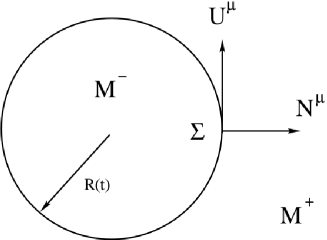
Figure 4.1: The spacetime is divided into two regions, the internal $M^{-}$ and external $M^{+}$, where $M^{-}=\left\{x^{\mu}:r<{\cal{R}}(t)\right\}$, and $M^{+}=\left\{x^{\mu}:r>{\cal{R}}(t)\right\}$. The surface $r={\cal{R}}(t)$ is denoted by $\Sigma$.

4.2.1 Preliminaries

We assume that the normal vector $\nabla\Phi$ to the hypersurface $\Sigma$ with components

$$\Phi_{,\lambda}=\delta_{\lambda}^{r}-\dot{\cal{R}}\delta^{t}_{\lambda},$$ (4.17)

$$\Phi^{,\lambda}=e^{-2\nu}(1-e^{2\mu}-\dot{\mathcal{R}}e^{\mu+\nu})\delta^{\lambda}_{r}+(e^{\mu-\nu}+\dot{\mathcal{R}})\delta_{t}^{\lambda},$$

is everywhere spacelike, i.e.

$$\Phi^{,\lambda}\Phi_{,\lambda}=e^{-2\nu}\bigl{[}1-(e^{\mu}+e^{\nu}\dot{\mathcal{R}})^{2}\bigr{]}>0.$$ (4.18)

This is the case if $\dot{\mathcal{R}}$ is small enough. We may then define the vector field $N=\nabla\Phi/\|\nabla\Phi\|_{g}$ in a neighborhood of $\Sigma$. The vector field $N$ should not be confused with the lapse function which in the present case is set to one, see Eq. (5.5). $N$ has length one, i.e. $N_{\lambda}N^{\lambda}=1$, and the restriction of $N$ to $\Sigma$ is the outward pointing unit normal vector field on $\Sigma$.

Let $H(\Phi)$ denote the Heaviside function defined by

$$H(\Phi)=\begin{cases}1,&\Phi>0,\\ \frac{1}{2},&\Phi=0,\\ 0,&\Phi<0,\end{cases}$$ (4.19)

and let $\delta(\Phi)$ denote the delta distribution with support on $\Sigma$. By definition, $\delta(\Phi)$ acts on a smooth test function $\varphi\in C^{\infty}(M)$ of compact support by

$$(\delta(\Phi),\varphi)=\int_{\Sigma}\varphi d\Sigma,$$ (4.20)

where $d\Sigma=\iota_{N}\text{Vol}_{g}$ is the volume three-form induced by $g$ on $\Sigma$ and $\iota_{N}$ denotes interior multiplication by $N$. The derivatives $\delta^{(n)}(\Phi)$, $n\geq 1$, of $\delta(\Phi)$ are defined in a standard way and the following relations are valid [119]:

$$\frac{\partial H(\Phi)}{\partial x^{\lambda}} = \frac{\partial\Phi}{\partial x^{\lambda}}\delta(\Phi),$$

$$\frac{\partial}{\partial x^{\lambda}}\delta^{(n)}(\Phi) = \frac{\partial\Phi}{\partial x^{\lambda}}\delta^{(n+1)}(\Phi),\qquad n=0,1,2,\dots,$$

$$\Phi\delta^{(n)}(\Phi) = -n\delta^{(n-1)}(\Phi),\qquad n=1,2,\dots.$$ (4.21)

If $f$ is a function defined in a neighborhood of $\Sigma$, we define the distribution $f\delta^{(n)}(\Phi)$ by letting it act on a test function $\varphi$ by

$$(f\delta^{(n)}(\Phi),\varphi)=(\delta^{(n)}(\Phi),f\varphi).$$ (4.22)

The product $f\delta(\Phi)$ is well defined whenever $f$ is $C^{0}$ and it depends only on the restriction $f|_{\Sigma}$ of $f$ to $\Sigma$. More generally, the product $f\delta^{(n)}(\Phi)$ is well defined provided that $f$ is $C^{n}$ and it depends only on the values of $f$ and its partial derivatives of order $\leq n$ evaluated on $\Sigma$.

Let $F$ be a distribution on $M$ of the form

$$F=F^{+}H(\Phi)+F^{-}[1-H(\Phi)]+\sum_{k=0}^{n}F^{Im(k)}\delta^{(k)}(\Phi),$$ (4.23)

where the $F_{n}$’s are functions defined in a neighborhood of $\Sigma$ while $F^{+}$ and $F^{-}$ are sufficiently smooth functions defined on $M^{+}$ and $M^{-}$ respectively. We define the function $F^{D}$ on $M$ by

$$F^{D}=F^{+}H(\Phi)+F^{-}[1-H(\Phi)],$$ (4.24)

and we define the jump $[F]^{-}$ of $F$ across $\Sigma$ by

$$[F]^{-}(x)=F^{+}(x)-F^{-}(x),\qquad x\in\Sigma.$$ (4.25)

We will also need the fact that the equation $F=0$ is equivalent to the equations

$$F^{\pm}(x)=0,\qquad x\in M^{\pm},$$ (4.26)

and

$$\sum_{k=0}^{j}(-1)^{k}\frac{(n-k)!j!}{(j-k)!}\frac{\partial^{j-k}}{\partial\Phi^{j-k}}F^{Im(n-k)}\bigg{|}_{\Sigma}=0,$$

$$\hskip 113.81102pt0\leq j\leq n,$$ (4.27)

where $\frac{\partial}{\partial\Phi}$ acts on a function $f$ by

$$\frac{\partial f}{\partial\Phi}=\frac{1}{\|\nabla\Phi\|_{g}}df\cdot N,$$ (4.28)

and, more generally, for any $j\geq 1$,

$$\frac{\partial^{j}f}{\partial\Phi^{j}}=\biggl{(}\frac{1}{\|\nabla\Phi\|_{g}}\iota_{N}d\biggr{)}^{j}f.$$ (4.29)

A proof of this fact is given at the end of the chapter.

For $n=3$, the conditions in (4.27) are

$$F^{Im(3)}|_{\Sigma}=0,$$

$$\biggl{(}3\frac{\partial F^{Im(3)}}{\partial\Phi}-F^{Im(2)}\biggr{)}\bigg{|}_{\Sigma}=0,$$

$$\biggl{(}3\frac{\partial^{2}F^{Im(3)}}{\partial\Phi^{2}}-2\frac{\partial F^{Im(2)}}{\partial\Phi}+F^{Im(1)}\biggr{)}\bigg{|}_{\Sigma}=0,$$ (4.30)

$$\biggl{(}\frac{\partial^{3}F^{Im(3)}}{\partial\Phi^{3}}-\frac{\partial^{2}F^{Im(2)}}{\partial\Phi^{2}}+\frac{\partial F^{Im(1)}}{\partial\Phi}-F^{Im(0)}\biggr{)}\bigg{|}_{\Sigma}=0.~{}~{}$$

Proof of Eqs. (4.26)–(4.27).

Let $F$ be given by (4.23). We will show that the equation $F=0$ is equivalent to the conditions (4.26) and (4.27). It is clear that the equation $F=0$ is equivalent to (4.26) together with the condition

$$\sum_{k=0}^{n}F^{Im(k)}\delta^{(k)}(\Phi)=0.$$ (4.31)

It remains to show that (4.31) is equivalent to (4.27).

Suppose first that (4.31) holds. Then, multiplying (4.31) by $\Phi^{n-j}$ and using the recursion relation (4.21) repeatedly, we find

$$G\delta^{(j)}(\Phi)=0,\qquad 0\leq j\leq n,$$ (4.32)

where the function $G$ is defined in a neighborhood of $\Sigma$ by

$$G(x)=\sum_{k=0}^{n}(-1)^{k}k!F^{Im(k)}(x)\Phi^{n-k}(x).$$ (4.33)

Equation (4.32) with $j=0$ implies that the restriction of $G$ to $\Sigma$ vanishes, i.e. $G|_{\Sigma}=0$. Equation (4.32) with $j=1$ then gives

$$0=G\delta^{\prime}(\Phi)=\frac{G}{\Phi}\Phi\delta^{\prime}(\Phi)=-\frac{G}{\Phi}\delta(\Phi)\quad\text{i.e.}\quad\frac{G}{\Phi}\Big{|}_{\Sigma}=0.$$

In terms of local coordinates $\{u^{j}\}$ such that $u^{1}=\Phi$ while the remaining coordinates $\{u^{j}\}_{j\geq 2}$ parametrize the level surfaces of $\Phi$, we have

$$0=\frac{G}{\Phi}\Big{|}_{\Sigma}=\frac{\partial G}{\partial\Phi}\bigg{|}_{\Phi=0}.$$

Thus, $G$ vanishes to the first order on $\Sigma$. Repeating the above procedure $n$ times, we infer that $G$ vanishes to the $n$th order on $\Sigma$:

$$\frac{G}{\Phi^{j}}\bigg{|}_{\Sigma}=0\quad\text{i.e.}\quad\frac{\partial^{j}G}{\partial\Phi^{j}}\bigg{|}_{\Phi=0}=0,\qquad 0\leq j\leq n.$$ (4.34)

The partial derivatives denoted in the local coordinates $(u^{j})$ by $\frac{\partial^{j}}{\partial\Phi^{j}}$ can be expressed invariantly as in (4.29). Substituting the expression (4.33) for $G$ into (4.34), we find

$$0 = \sum_{k=0}^{n}(-1)^{k}k!\sum_{r=0}^{j}{j\choose r}\frac{\partial^{j-r}F^{Im(k)}}{\partial\Phi^{j-r}}\frac{\partial^{r}\Phi^{n-k}}{\partial\Phi^{r}}\bigg{|}_{\Phi=0}$$

$$= \sum_{k=n-j}^{n}(-1)^{k}k!(n-k)!{j\choose n-k}\frac{\partial^{j-(n-k)}F^{Im(k)}}{\partial\Phi^{j-(n-k)}}\bigg{|}_{\Phi=0},$$

$$\hskip 113.81102pt\qquad 0\leq j\leq n.$$

Replacing $k$ by $n-k$, we find (4.27).

Conversely, if (4.27) holds, then tracing the above steps backwards, we infer that (4.32), and hence also (4.31), holds.

4.2.2 Distributional Metric Functions

The field equations (2.15)–(2.3) involve second-order derivatives of the metric coefficients with respect to $t$ and sixth-order derivatives with respect to $x^{i}$. Thus, one might require that the metric coefficients be $C^{1}$ with respect to $t$ and $C^{5}$ with respect to $x^{i}$, where $C^{n}$ indicates that the first $n$ derivatives exist and are continuous across the hypersurface $\Phi=0$. However, this assumption eliminates the important case of an infinitely thin shell of matter supported on $\Sigma$. Therefore, we will instead make weaker assumptions, so that a thin shell located on the hypersurface $\Phi=0$ is in general allowed, and consider the case without a thin shell only as a particular case of our general treatment to be provided below. In fact, we shall impose the minimal requirement that the corresponding problem be mathematically meaningful in terms of distribution theory. Then, in review of Eqs. (4.4)–(4.12), we find that the cases $\lambda=1$ and $\lambda\not=1$ have different dependencies on the derivatives of $\mu$. In particular, the term $\mu^{\prime}\mu^{\prime\prime}$ appears when $\lambda\not=1$. Thus, in the following we consider the two cases separately.

$\lambda=1.$

In this case, we assume that: (a) $\mu$ and $\nu$ are $C^{5}$ in each of the regions $M^{+}$ and $M^{-}$ up to the boundary $\Sigma$; (b) $\mu$ is $C^{0}$ across $\Sigma$; (c) $\nu$ is $C^{0}$ with respect to $t$ and $C^{2}$ with respect to $r$ across $\Sigma$.

The above regularity assumptions ensure that the mathematically ill-defined products $\delta(\Phi)^{2}$ and $\delta(\Phi)H(\Phi)$ do not appear in the field equations. Indeed, the terms in the field equations (4.4)–(4.12) that could lead to products of this type are

$${\mu^{\prime}}^{2},\;\;\dot{\mu}\mu^{\prime},\;\;\dot{\nu}^{2},\;\;{\nu^{\prime\prime}}^{2},\;\;\nu^{\prime\prime}\nu^{\prime\prime\prime}.$$ (4.35)

Our assumptions imply that these terms may contain $H(\Phi)^{2}$ but not $\delta(\Phi)^{2}$ or $\delta(\Phi)H(\Phi)$.

In order to compute the derivatives of $\mu$ and $\nu$, we note that

$$\mu = \mu^{D}=\mu^{+}H(\Phi)+\mu^{-}[1-H(\Phi)],$$

$$\nu = \nu^{D}=\nu^{+}H(\Phi)+\nu^{-}[1-H(\Phi)],$$ (4.36)

where the functions $\mu^{+}$ and $\nu^{+}$ are $C^{5}$ on $M^{+}$, while the functions $\mu^{-}$ and $\nu^{-}$ are $C^{5}$ on $M^{-}$. Let $V_{\Sigma}$ denote an open neighborhood of $\Sigma$. Let $\tilde{\mu}^{+}$ and $\tilde{\nu}^{+}$ denote $C^{5}$-extensions of $\mu^{+}$ and $\nu^{+}$ to $M^{+}\cup V_{\Sigma}$. Let $\tilde{\mu}^{-}$ and $\tilde{\nu}^{-}$ denote $C^{5}$-extensions of $\mu^{-}$ and $\nu^{-}$ to $M^{-}\cup V_{\Sigma}$. Then the functions

$$\hat{\mu}\equiv\tilde{\mu}^{+}-\tilde{\mu}^{-},\qquad\hat{\nu}\equiv\tilde{\nu}^{+}-\tilde{\nu}^{-},$$ (4.37)

are defined on $V_{\Sigma}$ and the following relations are valid on $\Sigma$ whenever $\alpha+\beta\leq 5$:

$$\hat{\mu}=[\mu]^{-},\quad\frac{\partial^{\alpha+\beta}}{\partial t^{\alpha}\partial r^{\beta}}\hat{\mu}=\biggl{[}\frac{\partial^{\alpha+\beta}}{\partial t^{\alpha}\partial r^{\beta}}\mu\biggr{]}^{-},$$ (4.38)

$$\hat{\nu}=[\nu]^{-},\quad\frac{\partial^{\alpha+\beta}}{\partial t^{\alpha}\partial r^{\beta}}\hat{\nu}=\biggl{[}\frac{\partial^{\alpha+\beta}}{\partial t^{\alpha}\partial r^{\beta}}\nu\biggr{]}^{-}.$$ (4.39)

Since $\mu$ is $C^{0}$ across $\Sigma$, we find

$$\mu_{,t} = (\mu_{,t})^{D},$$

$$\mu_{,r} = (\mu_{,r})^{D},$$

$$\mu_{,tr} = (\mu_{,tr})^{D}+\hat{\mu}_{,t}\delta(\Phi),$$

$$\mu_{,rt} = (\mu_{,rt})^{D}-\dot{\cal{R}}\hat{\mu}_{,r}\delta(\Phi),$$

$$\mu_{,rr} = (\mu_{,rr})^{D}+\hat{\mu}_{,r}\delta(\Phi).$$

$$\mu_{,rrr} = (\mu_{,rrr})^{D}+2\hat{\mu}_{,rr}\delta(\Phi)+\hat{\mu}_{,r}\delta^{\prime}(\Phi).$$ (4.40)

Since $\mu$ is $C^{0}$ across $\Sigma$, the derivatives of $\mu^{+}$ and $\mu^{-}$ in any direction tangential to $\Sigma$ must coincide when evaluated on $\Sigma$. In particular, since the vector $U$ defined by

$$U^{\lambda}\equiv\delta^{\lambda}_{t}+\dot{\cal{R}}\delta^{\lambda}_{r},$$ (4.41)

is tangential to $\Sigma$ (i.e. $U^{\lambda}N_{\lambda}=0$), we obtain

$$U^{\lambda}[\mu_{,\lambda}]^{-}=[\mu_{,t}]^{-}+\dot{\cal{R}}[\mu_{,r}]^{-}=0,$$

that is,

$$\hat{\mu}_{,t}=-\dot{\cal{R}}\hat{\mu}_{,r},$$ (4.42)

after Eq. (5.30) is taken into account. Then, from Eq. (4.40) one finds $\mu_{,tr}=\mu_{rt}$, as it is expected.

Similarly, since $\nu$ is $C^{0}$ across $\Sigma$, we also have

$$0=U^{\lambda}[\nu_{,\lambda}]^{-}=[\nu_{,t}]^{-}+\dot{\cal{R}}[\nu_{,r}]^{-}.$$ (4.43)

But $[\nu_{,r}]^{-}=0$, because $\nu$ is assumed to be $C^{2}$ with respect to $r$. Thus $[\nu_{,t}]^{-}=0$. Therefore, $\nu$ is in fact $C^{1}$ across $\Sigma$. The same argument applied to $\nu_{,t}$ and $\nu_{,r}$ now implies that $\nu$ is in fact $C^{2}$ across $\Sigma$. We find

$$\nu_{,t} = (\nu_{,t})^{D},$$

$$\nu_{,r} = (\nu_{,r})^{D},$$

$$\nu_{,rr} = (\nu_{,rr})^{D},$$

$$\nu^{(3)} = (\nu^{(3)})^{D},$$

$$\nu^{(4)} = (\nu^{(4)})^{D}+\hat{\nu}^{(3)}\delta(\Phi),$$

$$\nu^{(5)} = (\nu^{(5)})^{D}+2\hat{\nu}^{(4)}\delta(\Phi)+\hat{\nu}^{(3)}\delta^{\prime}(\Phi),$$ (4.44)

where $\nu^{(n)}\equiv\partial^{n}\nu/\partial r^{n}$. We emphasize that the expressions on the right-hand sides of (4.40) and (4.44) are independent of the extensions used to define $\hat{\mu}$ and $\hat{\nu}$ in (4.37), because the values of $\hat{\mu}$, $\hat{\nu}$, and their partial derivatives of order $\leq 5$ are uniquely prescribed on $\Sigma$ in view of (4.39).

The Junction Conditions.

We will find the junction conditions across $\Sigma$ by substituting the expressions (4.40) and (4.44) for the derivatives of $\mu$ and $\nu$ into the field equations (4.4)–(4.12).

Table 4.1: A list of all field equations for $\lambda=1$.

Variation		General	Spherically	Junction
w. r. t.	Name of equation	version	symmetric case	condition
lapse $N(t)$	Hamiltonian      constraint	(2.15)	(4.4)	(4.46)
shift $N^{i}$	Momentum        constraint	(2.17)	(4.1)	(4.47)
$\varphi$	-	(2.19)	(4.1)	(4.47)
gauge field $A$	-	(2.20)	(4.7)	(4.47)
metric $g_{ij}$	Dynamical        equations	(2.3)	(4.1) and (4.1)	(4.48) and (4.2.2)
-	Energy                    conservation law	(2.3)	(4.11)	(4.50)
-	Momentum        conservation law	(2.3)	(4.12)	(4.2.2)

Suppose that the energy density $\rho_{H}=-2J^{t}$ has the form

$$\rho_{H}=(\rho_{H})^{D}+\sum_{n=0}^{\infty}\rho_{H}^{Im(n)}\delta^{(n)}(\Phi),$$ (4.45)

where it is understood that only finitely many of the $\rho_{H}^{Im(n)}$’s are nonzero. Since, by (4.1),

$$\mathcal{L}_{K}=(\mathcal{L}_{K})^{D},\qquad\mathcal{L}_{V}=(\mathcal{L}_{V})^{D},$$

the Hamiltonian constraint (4.4) reads

$$\int_{r<\mathcal{R}(t)}\left(\mathcal{L}_{K}^{-}+\mathcal{L}_{V}^{-}+4\pi G\rho_{H}^{-}\right)e^{\nu}r^{2}dr$$

$$+\int_{r>\mathcal{R}(t)}\left({\cal{L}}_{K}^{+}+{\cal{L}}_{V}^{+}+4\pi G\rho_{H}^{+}\right)e^{\nu}r^{2}dr$$ (4.46)

$$+4\pi G\sum_{n=0}^{\infty}(-1)^{n}\frac{\partial^{n}}{\partial r^{n}}\bigg{|}_{r=\mathcal{R}(t)}\bigl{(}\rho_{H}^{Im(n)}e^{\nu}r^{2}\bigr{)}=0.$$

The left-hand sides of Eqs. (4.1), (4.1) and (4.7) have no supports on the hypersurface $r={\cal{R}}(t)$. Thus, these equations remain unchanged in the regions $M^{+}$ and $M^{-}$, while on the hypersurface $\Sigma$ they yield

$$v=v^{D},\qquad J_{\varphi}=(J_{\varphi})^{D},\qquad J_{A}=(J_{A})^{D}.$$ (4.47)

In fact, in order to avoid that the ill-defined product $H(\Phi)\delta(\Phi)$ arises from the term $J_{A}A^{\prime}$ in (4.12), we will assume that $J_{A}$ is $C^{0}$.

The gauge field $A$ has dimension $[A]=4$, so the action cannot contain terms like $A^{n}$ with $n\geq 2$, that is, it must be linear in $A$. We therefore assume that $A$ has the form

$$A(t,r) = A^{D}+\sum_{n=0}^{\infty}A^{Im(n)}\delta^{(n)}(\Phi).$$

It follows that

$$A_{,r} = (A_{,r})^{D}+\bigl{[}\hat{A}+A_{,r}^{Im(0)}\bigr{]}\delta(\Phi)+\sum_{n=1}^{\infty}\bigl{[}A_{,r}^{Im(n)}+A^{Im(n-1)}\bigr{]}\delta^{(n)}(\Phi),$$

$$A_{,rr} = (A_{,rr})^{D}+\bigl{[}2\hat{A}_{,r}+A_{,rr}^{Im(0)}\bigr{]}\delta(\Phi)+\bigl{[}\hat{A}+2A_{,r}^{Im(0)}+A_{,rr}^{Im(1)}\bigr{]}\delta^{\prime}(\Phi)$$

$$+\sum_{n=2}^{\infty}\bigl{[}A_{,rr}^{Im(n)}+2A_{,r}^{Im(n-1)}+A^{Im(n-2)}\bigr{]}\delta^{(n)}(\Phi).$$

Thus,

$$F_{rr}^{A} = \frac{2}{r}\biggl{\{}(A_{,r})^{D}+\nu_{,r}A^{D}+\bigl{[}\hat{A}+A_{,r}^{Im(0)}+\nu_{,r}A^{Im(0)}\bigr{]}\delta(\Phi)$$

$$+\sum_{n=1}^{\infty}\Bigl{[}\bigl{(}A_{,r}^{Im(n)}+A^{Im(n-1)}\bigr{)}\delta^{(n)}(\Phi)+\nu_{,r}A^{Im(n)}\delta^{(n)}(\Phi)\Bigr{]}\biggr{\}},$$

$$F_{\theta\theta}^{A} = (F_{\theta\theta}^{A})^{D}+\sum_{n=0}^{\infty}F_{\theta\theta}^{A,Im(n)}\delta^{(n)}(\Phi),$$

where

$$(F_{\theta\theta}^{A})^{D} = e^{-2\nu}\bigl{[}r^{2}(A_{,rr})^{D}-\nu_{,r}r^{2}(A_{,r})^{D}+r(A_{,r})^{D}+r\nu_{,r}A^{D}-(1-e^{2\nu})A^{D}\bigr{]},$$

$$F_{\theta\theta}^{A,Im(0)} = e^{-2\nu}\bigl{[}r^{2}(2\hat{A}_{,r}+A_{,rr}^{Im(0)})-r^{2}\nu_{,r}(\hat{A}+A_{,r}^{Im(0)})$$

$$+r(\hat{A}+A_{,r}^{Im(0)})+r\nu_{,r}A^{Im(0)}-(1-e^{2\nu})A^{Im(0)}\bigr{]},$$

$$F_{\theta\theta}^{A,Im(1)} = e^{-2\nu}\bigl{[}r^{2}(\hat{A}+2A_{,r}^{Im(0)}+A_{,rr}^{Im(1)})-r^{2}\nu_{,r}(A^{Im(0)}+A_{,r}^{Im(1)})$$

$$+r(A^{Im(0)}+A_{,r}^{Im(1)})+r\nu_{,r}A^{Im(1)}-(1-e^{2\nu})A^{Im(1)}\bigr{]},$$

$$F_{\theta\theta}^{A,Im(n)} = e^{-2\nu}\bigl{[}r^{2}\big{(}A^{Im(n-2)}+2A_{,r}^{Im(n-1)}+A_{,rr}^{Im(n)}\big{)}-r^{2}\nu_{,r}(A^{Im(n-1)}+A_{,r}^{Im(n)})$$

$$+r(A^{Im(n-1)}+A_{,r}^{Im(n)})+r\nu_{,r}A^{Im(n)}-(1-e^{2\nu})A^{Im(n)}\bigr{]},\;n\geq 2.$$

From Eq. (4.1) we find that the functions $\{F_{n}\}_{n=1}^{6}$ contain no delta functions whereas

$$(F_{7})_{rr} = (F_{7})_{rr}^{D}-\frac{16e^{-4\nu}}{r^{2}}\hat{\nu}^{(3)}\delta(\Phi),$$

$$(F_{8})_{rr} = (F_{8})_{rr}^{D}-\frac{6e^{-4\nu}}{r^{2}}\hat{\nu}^{(3)}\delta(\Phi),$$

$$(F_{7})_{\theta\theta} = (F_{7})_{\theta\theta}^{D}-8re^{-6\nu}\bigl{[}(2\hat{\nu}^{(4)}-16\nu_{,r}\hat{\nu}^{(3)})\delta(\Phi)+\hat{\nu}^{(3)}\delta^{\prime}(\Phi)\bigr{]},$$

$$(F_{8})_{\theta\theta} = (F_{8})_{\theta\theta}^{D}-3re^{-6\nu}\bigl{[}(2\hat{\nu}^{(4)}-16\nu_{,r}\hat{\nu}^{(3)})\delta(\Phi)+\hat{\nu}^{(3)}\delta^{\prime}(\Phi)\bigr{]}.$$

Thus, (2.3) gives

$$F_{rr} = (F_{rr})^{D}-(16g_{7}+6g_{8})\frac{e^{-4\nu}}{r^{2}\zeta^{4}}\hat{\nu}^{(3)}\delta(\Phi),$$

$$F_{\theta\theta} = (F_{\theta\theta})^{D}-(8g_{7}+3g_{8})\frac{re^{-6\nu}}{\zeta^{4}}\bigl{[}(2\hat{\nu}^{(4)}-16\nu_{,r}\hat{\nu}^{(3)})\delta(\Phi)+\hat{\nu}^{(3)}\delta^{\prime}(\Phi)\bigr{]}.$$

Writing $p_{r}$ in the form

$$p_{r}(t,r)=p_{r}^{D}+\sum_{n=0}^{\infty}p_{r}^{Im(n)}\delta^{(n)}(\Phi),$$

we find that Eq. (4.1) remains unchanged in the regions $M^{+}$ and $M^{-}$, while on the hypersurface $\Sigma$ it yields

$$\sum_{n=0}^{\infty} \biggl{\{}\frac{e^{2\nu}}{r}[e^{-2\nu}(1-2r\nu^{\prime})+\Lambda_{g}r^{2}-1]A^{Im(n)}$$ (4.48)

$$+r\Bigl{[}F_{rr}^{Im(n)}+F_{rr}^{AIm(n)}+8\pi Ge^{2\nu}p_{r}^{Im(n)}\Bigr{]}\biggr{\}}$$

$$~{}~{}~{}~{}~{}~{}~{}~{}~{}\times\delta^{(n)}(\Phi)=0.$$

Using (4.27), Eq. (4.48) can be rewritten as a hierarchy of scalar equations on $\Sigma$.

Similarly, Eq. (4.1) remains unchanged in the regions $M^{+}$ and $M^{-}$, while on the hypersurface $\Sigma$ it yields

$$r(\hat{\mu}_{,r}e^{2\mu}+\dot{\mathcal{R}}\hat{\mu}_{,r}e^{\nu+\mu})\delta(\Phi)$$

$$+\sum_{n=0}^{\infty}\biggl{\{}\frac{e^{2\nu}}{r}[e^{-2\nu}(1-2r\nu^{\prime})+\Lambda_{g}r^{2}-1]A^{Im(n)}$$

$$+\frac{e^{2\nu}}{r}\Bigl{[}F_{\theta\theta}^{Im(n)}+F_{\theta\theta}^{AIm(n)}+8\pi Gr^{2}p_{\theta}^{Im(n)}\Bigr{]}\biggr{\}}\delta^{(n)}(\Phi)=0.$$

Note that

$$\rho_{H,t} = (\rho_{H,t})^{D}+\bigl{[}\rho_{H,t}^{Im(0)}-\dot{\mathcal{R}}\hat{\rho}_{H}\bigr{]}\delta(\Phi)+\sum_{n=1}^{\infty}\bigl{(}\rho_{H,t}^{Im(n)}-\dot{\mathcal{R}}\rho_{H}^{Im(n-1)}\bigr{)}\delta^{(n)}(\Phi),$$

and, by (4.47),

$$v_{,t} = (v_{,t})^{D}-\dot{\mathcal{R}}\hat{v}\delta(\Phi).$$

Thus, in view of (4.47), the energy conservation law (4.11) takes the form

$$\int dr\,e^{\nu}r^{2}\Bigl{\{} (\rho_{H,t})^{D}+\bigl{[}\rho_{H,t}^{Im(0)}-\dot{\mathcal{R}}\hat{\rho}_{H}\bigr{]}\delta(\Phi)$$

$$+\sum_{n=1}^{\infty}\bigl{(}\rho_{H,t}^{Im(n)}-\dot{\mathcal{R}}\rho_{H}^{Im(n-1)}\bigr{)}\delta^{(n)}(\Phi)$$

$$+\biggl{(}(\rho_{H})^{D}+\sum_{n=0}^{\infty}\rho_{H}^{Im(n)}\delta^{(n)}(\Phi)$$

$$+4(p_{r})^{D}+4\sum_{n=0}^{\infty}p_{r}^{Im(n)}\delta^{(n)}(\Phi)\biggr{)}\nu_{,t}$$

$$+4((v_{,t})^{D}-\dot{\mathcal{R}}\hat{v}\delta(\Phi)-v^{D}\mu_{,t})$$

$$-2\bigl{(}(J_{A,t})^{D}+\nu_{,t}(J_{A})^{D}\bigr{)}\Bigr{\}}=0,$$

that is,

$$\biggl{(}\int_{r<\mathcal{R}(t)}+\int_{r>\mathcal{R}(t)}\biggr{)}e^{\mu}r^{2}\bigl{(}\rho_{H,t}+\nu_{,t}(\rho_{H}+4p_{r})$$

$$+4v_{,t}-4v\mu_{,t}-2(J_{A,t}+\nu_{,t}J_{A})\bigr{)}dr+\Bigl{[}e^{\nu}r^{2}\Bigl{(}\rho_{H,t}^{Im(0)}$$

$$-\dot{\mathcal{R}}\hat{\rho}_{H}+\nu_{,t}\bigl{(}\rho_{H}^{Im(0)}+4p_{r}^{Im(0)}\bigr{)}-4\dot{\mathcal{R}}\hat{v}\Bigr{)}\Bigr{]}\Big{|}_{r=\mathcal{R}(t)}$$

$$+\sum_{n=1}^{\infty}(-1)^{n}\frac{\partial^{n}}{\partial r^{n}}\bigg{|}_{r=\mathcal{R}(t)}\Bigl{[}e^{\nu}r^{2}\Bigl{(}\rho_{H,t}^{Im(n)}-\dot{\mathcal{R}}\rho_{H}^{Im(n-1)}$$

$$+\nu_{,t}\bigl{(}\rho_{H}^{Im(n)}+4p_{r}^{Im(n)}\bigr{)}\Bigr{)}\Bigr{]}=0.$$ (4.50)

The momentum conservation law (4.12) remains unchanged in $M^{+}$ and $M^{-}$ while on the hypersurface $\Sigma$ it yields

$$-\hat{v}\delta(\Phi)+\hat{p}_{r}\delta(\Phi)+\sum_{n=0}^{\infty}\bigl{[}(p_{r}^{Im(n)})_{,r}\delta^{(n)}(\Phi)+p_{r}^{Im(n)}\delta^{(n+1)}(\Phi)\bigr{]}$$

$$+\frac{2}{r}\sum_{n=0}^{\infty}(p_{r}^{Im(n)}-p_{\theta}^{Im(n)})\delta^{(n)}(\Phi)-\frac{1}{2}J_{A}\biggl{[}\bigl{(}\hat{A}+A_{,r}^{Im(0)}\bigr{)}\delta(\Phi)$$

$$+\sum_{n=1}^{\infty}\bigl{(}A_{,r}^{Im(n)}+A^{Im(n-1)}\bigr{)}\delta^{(n)}(\Phi)\biggr{]}+e^{\nu-\mu}\dot{\mathcal{R}}\hat{v}\delta(\Phi)=0,$$

where we have used that

$$p_{r}^{\prime}=\hat{p}_{r}\delta(\Phi)+\sum_{n=0}^{\infty}\bigl{[}(p_{r}^{Im(n)})_{,r}\delta^{(n)}(\Phi)+p_{r}^{Im(n)}\delta^{(n+1)}(\Phi)\bigr{]}.$$

This completes the general description of the junction conditions for the case $\lambda=1$, which are summarized in Table 1.

$\lambda\not=1.$

In this case, the nonlinear terms

$${\mu^{\prime}}^{2},\;\;\dot{\mu}\mu^{\prime},\;\;\mu^{\prime}\mu^{\prime\prime},\;\;\dot{\nu}^{2},\;\;{\nu^{\prime\prime}}^{2},\;\;\nu^{\prime\prime}\nu^{\prime\prime\prime},$$ (4.51)

appear in the field equations (4.4)–(4.12). Thus, to ensure these field equations are well-defined, we assume that: (a) $\mu$ and $\nu$ are $C^{5}$ in each of the regions $M^{+}$ and $M^{-}$ up to the boundary $\Sigma$; (b) $\mu$ is $C^{0}$ with respect to $t$ and $C^{1}$ with respect to $r$ across $\Sigma$; (c) $\nu$ is $C^{0}$ with respect to $t$ and $C^{2}$ with respect to $r$ across $\Sigma$.

The same argument as above shows that $\nu$ is $C^{2}$ and that $\mu$ is $C^{1}$ across $\Sigma$. Equations (4.40) and (4.44) for the derivatives of $\mu$ and $\nu$ are still valid, but since $\mu$ now is $C^{1}$, we have $\hat{\mu}_{,t}=\hat{\mu}_{,r}=0$. It follows that all the junction conditions (4.46)–(4.2.2) remain unchanged, except that the presence of the term $\mu^{\prime\prime\prime}$ in (4.1) implies that the expression for $J_{\varphi}$ now may include a delta function:

$$J_{\varphi}=(J_{\varphi})^{D}+(1-\lambda)\frac{e^{\mu-3\nu}}{4\pi G}\hat{\mu}_{,rr}\delta(\Phi).$$ (4.52)

In what follows, we will consider some specific models of gravitational collapse for which the spacetime inside the collapsing sphere is described by the Friedman-Lemaitre-Robertson-Walker (FLRW) universe.

4.3 Gravitational Collapse of Homogeneous and Isotropic Perfect Fluid

In this section, we consider the gravitational collapse of a spherical cloud consisting of a homogeneous and isotropic perfect fluid described by the FLRW universe. Gravitational collapse of a homogeneous and isotropic dust fluid filled in the whole space-time was considered in [120], using a method proposed in [121]:

$$ds^{2}=-d\bar{t}^{2}+a^{2}(\bar{t})\bigg{(}\frac{d\bar{r}^{2}}{1-k\bar{r}^{2}}+\bar{r}^{2}d^{2}\Omega\biggr{)},$$

where $k=0,\pm 1$. Letting $r=a(\bar{t})\bar{r},\;t=\bar{t}$, the corresponding ADM variables take the form (5.5) with $N^{-}=1$, and

$$\nu^{-}(t,r) = -\frac{1}{2}\ln\biggl{(}1-k\frac{r^{2}}{a^{2}(t)}\biggr{)},$$

$$\mu^{-}(t,r) = \ln\biggl{(}\frac{-\dot{a}(t)r}{\sqrt{a^{2}(t)-kr^{2}}}\biggr{)},$$ (4.53)

where $\dot{a}\leq 0$ for a collapsing cloud. For a perfect fluid, we assume that

$$p_{\theta}^{-}=p_{r}^{-}=p^{-}(t),\;\;\;v=0.$$ (4.54)

We anticipate that the junction condition for $\nu$ requires $k=0$. Then, we find that

$$\nu^{-}(t,r)=0,\qquad\mu^{-}(t,r)=\ln\big{(}{-rH}\big{)},\quad(k=0),\quad$$ (4.55)

where $H\equiv\dot{a}(t)/a(t)$, and that

$$\mathcal{L}_{K}^{-}={3(1-3\lambda)H^{2}},\;\;\;\mathcal{L}_{V}^{-}=2\Lambda,$$

$$\mathcal{L}_{\varphi}^{-}=\mathcal{L}_{\lambda}^{-}=0,\;\;\;\mathcal{L}_{A}^{-}=2\Lambda_{g}A^{-}.$$ (4.56)

It is easy to verify that the momentum constraint (4.1) is satisfied, whereas the equations (4.1) and (4.7) obtained by variation with respect to $\varphi$ and $A$ respectively, reduce to

$${3\Lambda_{g}H}+8\pi GJ_{\varphi}^{-} = 0,$$ (4.57)

$$4\pi GJ_{A}^{-}+\Lambda_{g} = 0.$$

Since $\nu^{-}=0$, we have $F_{ij}^{-}=-\Lambda g_{ij}^{-}$, and the first dynamical equation (4.1) reduces to the condition

$$\frac{4}{r}a^{2}A^{-}_{,r}+2a^{2}\Lambda_{g}{A^{-}}+2(3\lambda-1)a\ddot{a}+(3\lambda-1)\dot{a}^{2}+2a^{2}(8\pi Gp^{-}-\Lambda)=0.$$

If this condition is satisfied the second dynamical equation (4.1) also holds provided that $A^{-}_{,r}-rA^{-}_{,rr}=0.$ On the other hand, the momentum conservation law (4.12) reduces to $J_{A}^{-}A^{-}_{,r}=0.$ We conclude that the general solution when $k=0$ is given by

$$J_{\varphi}^{-}=-\frac{3\Lambda_{g}H}{8\pi G},\quad J_{A}^{-}=-\frac{\Lambda_{g}}{4\pi G},$$ (4.58)

with $A^{-}=A^{-}(t)$ being given by

$$\Lambda_{g}A^{-}+(3\lambda-1)\left(\frac{\ddot{a}}{a}+\frac{H^{2}}{2}\right)-\Lambda=-8\pi Gp^{-}.~{}~{}~{}~{}$$ (4.59)

In the rest of this section, we consider only the case where $\Lambda_{g}=0$. Then, Eq. (4.58) yields

$$J_{A}^{-}=J_{\varphi}^{-}=0,$$ (4.60)

for which Eq. (4.59) shows that now $A^{-}(t)$ is an arbitrary function of $t$, and $a(t)$ is given by

$$(3\lambda-1)\left(\frac{\ddot{a}}{a}+\frac{H^{2}}{2}\right)-\Lambda=-8\pi Gp^{-}.$$ (4.61)

It is interesting to note that, since the Hamiltonian constraint is global, there is no analog of the Friedman equation in the current situation. This is in contrast to the case of HL cosmology [76], where a Friedman-like equation still exists, because of the homogeneity and isotropy of the whole universe. Although there is no analog of the Birkhoff theorem in HL theory, so that the spacetime outside the collapsing cloud can be either static or dynamical, we assume in this chapter that the exterior solution is a static spherically symmetric vacuum spacetime. We also assume that the value of $\Lambda_{g}$ is the same in the exterior and interior regions, i.e.

$$\Lambda_{g}^{+}=\Lambda_{g}^{-}=0.$$ (4.62)

It is convenient to consider the cases $\lambda=1$ and $\lambda\not=1$ separately.

4.3.1 Gravitational Collapse with $\lambda=1$

We first consider the case of $\lambda=1$. In this case, the static spherically symmetric exterior vacuum solution has the form  [78]

$$\mu^{+}=\mu^{+}(r)=\frac{1}{2}\ln\biggl{(}\frac{2m^{+}}{r}+\frac{1}{3}\Lambda r^{2}-2A^{+}(r)+\frac{2}{r}\int_{r_{0}}^{r}A^{+}(r^{\prime})dr^{\prime}\biggr{)},$$

$$\nu^{+}=0,$$ (4.63)

for which we find that

$$\mathcal{L}_{K}^{+}=\frac{4}{r}A^{+}_{,r}-2\Lambda,\quad\mathcal{L}_{V}^{+}=2\Lambda,\quad\mathcal{L}_{A}^{+}=0,$$

$$v^{+}=J_{A}^{+}=J_{\varphi}^{+}=\rho_{H}^{+}=0,$$ (4.64)

where $m^{+}$, $r_{0}$ are constants and $A^{+}=A^{+}(r)$ is a function of $r$ only, yet to be determined.

As mentioned previously, the condition that $\nu$ be continuous across $\Sigma$ implies that $k=0$. We let the interior solution be of the form (4.55), and assume that the thin shell of matter separating the interior and exterior solutions is such that

$$p=p_{r}^{-},\quad v=0,\quad J_{\varphi}=J_{\varphi}^{Im(0)}\delta(\Phi),$$

$$p_{\theta}=p_{\theta}^{-}+p_{\theta}^{Im(0)}\delta(\Phi),\quad\rho_{H}=\rho_{H}^{-}+\rho_{H}^{Im(0)}\delta(\Phi),\quad$$

$$A=A^{D}+A^{Im(0)}\delta(\Phi),\quad J_{A}=0,$$ (4.65)

where $\rho^{+}_{H}=J_{\varphi}^{\pm}=p_{\theta}^{+}=p_{r}^{+}=0$.

Proposition 4.1.

For the spacetime defined by (4.55), (4.61), (4.3.1), the six junction conditions (4.46)–(4.2.2) reduce to the following six conditions:

$$\left(-6H^{2}+2\Lambda+4\pi G\rho_{H}^{-}(t)\right)\frac{\mathcal{R}(t)^{3}}{3}+4\int_{\mathcal{R}(t)}^{\infty}A_{,r}^{+}rdr+4\pi G\rho_{H}^{Im(0)}r^{2}\Big{|}_{r=\mathcal{R}(t)}=0,$$ (4.66)

$$J_{\varphi}^{Im(0)}=0,$$ (4.67)

$$\text{$A(t,r)$ is continuous across $\Sigma$},$$ (4.68)

$$A_{,t}^{-}=\mathcal{R}\biggl{(}\frac{\Lambda}{2}-H^{2}\biggr{)}(\dot{\mathcal{R}}-H\mathcal{R})-8\pi Gp_{\theta}^{Im(0)}H\mathcal{R},$$ (4.69)

$$\rho_{H}^{Im(0)}(t,\mathcal{R}(t))=e^{-\int_{0}^{t}\frac{2\dot{\mathcal{R}}(\tau)}{\mathcal{R}(\tau)}d\tau}\biggl{[}\rho_{H}^{Im(0)}(0,\mathcal{R}(0))+\int_{0}^{t}e^{\int_{0}^{s}\frac{2\dot{\mathcal{R}}(\tau)}{\mathcal{R}(\tau)}d\tau}\biggl{(}\frac{1}{4}H(s)\mathcal{R}(s)^{2}\rho_{H,t}^{-}(s)$$

$$~{}~{}~{}~{}~{}~{}~{}~{}~{}~{}~{}~{}~{}~{}~{}~{}~{}~{}~{}~{}~{}~{}~{}-\dot{\mathcal{R}}(s)\rho_{H}^{-}(s)\biggr{)}ds\biggr{]},$$ (4.70)

$$\text{$rp+2p_{\theta}^{Im(0)}=0$ on $\Sigma$}.$$ (4.71)

Moreover, the condition that $\mu$ be continuous across $\Sigma$ implies that

$$A^{-}_{,t}=\frac{\Lambda-3H^{2}}{2}\mathcal{R}\dot{\mathcal{R}}-HH_{,t}\mathcal{R}^{2}.$$ (4.72)

Proof.  For the spacetime defined by (4.3.1)–(4.65), condition (4.46) reduces to

$$\left(-6H(t)^{2}+2\Lambda+4\pi G\rho_{H}^{-}(t)\right)\int_{0}^{\mathcal{R}(t)}r^{2}dr+4\int_{\mathcal{R}(t)}^{\infty}A_{,r}^{+}rdr+4\pi G\rho_{H}^{Im(0)}r^{2}\Big{|}_{r=\mathcal{R}(t)}=0,$$

which yields (4.66). Moreover, condition (4.47) reduces immediately to (4.67).

Conditions (4.48) and (4.2.2) reduce to

$$F_{rr}^{AIm(0)}\delta(\Phi)+F_{rr}^{AIm(1)}\delta^{\prime}(\Phi)=0,$$ (4.73)

and

$$r(\hat{\mu}_{,r}e^{2\mu}+\dot{\mathcal{R}}\hat{\mu}_{,r}e^{\mu})\delta(\Phi)$$

$$+\frac{1}{r}F_{\theta\theta}^{AIm(0)}\delta(\Phi)+\frac{1}{r}F_{\theta\theta}^{AIm(1)}\delta^{\prime}(\Phi)$$

$$+\frac{1}{r}F_{\theta\theta}^{AIm(2)}\delta^{\prime\prime}(\Phi)+8\pi Grp_{\theta}^{Im(0)}\delta(\Phi)=0,$$ (4.74)

respectively, where we have used that

$$F_{rr}=(F_{rr})^{D},\qquad F_{\theta\theta}=(F_{\theta\theta})^{D}.$$ (4.75)

Now

$$F_{rr}^{A} = \frac{2}{r}\biggl{\{}(A_{,r})^{D}+\bigl{[}\hat{A}+A_{,r}^{Im(0)}\bigr{]}\delta(\Phi)+A^{Im(0)}\delta^{\prime}(\Phi)\biggr{\}},$$

$$F_{\theta\theta}^{A} = (F_{\theta\theta}^{A})^{D}+\sum_{n=0}^{2}F_{\theta\theta}^{A,Im(n)}\delta^{(n)}(\Phi),$$ (4.76)

where

$$(F_{\theta\theta}^{A})^{D} = r^{2}(A_{,rr})^{D}+r(A_{,r})^{D},$$

$$F_{\theta\theta}^{A,Im(0)} = r^{2}(2\hat{A}_{,r}+A_{,rr}^{Im(0)})+r(\hat{A}+A_{,r}^{Im(0)}),$$

$$F_{\theta\theta}^{A,Im(1)} = r^{2}(\hat{A}+2A_{,r}^{Im(0)})+rA^{Im(0)},$$

$$F_{\theta\theta}^{A,Im(2)} = r^{2}A^{Im(0)}.$$

Thus, equation (4.73) can be written as

$$\bigl{[}\hat{A}+A_{,r}^{Im(0)}\bigr{]}\delta(\Phi)+A^{Im(0)}\delta^{\prime}(\Phi)=0.$$ (4.77)

Thus, by (4.30), $A^{Im(0)}|_{\Sigma}=0$. Hence, $A^{Im(0)}\delta(\Phi)=0$ which gives

$$0=(A^{Im(0)}\delta(\Phi))_{,r}=A_{,r}^{Im(0)}\delta(\Phi)+A^{Im(0)}\delta^{\prime}(\Phi).$$

Equation (4.77) then gives $\hat{A}|_{\Sigma}=0$ so that in fact $A$ is continuous across $\Sigma$, which proves (4.68). Equation (4.74) can now be written as

$$\Bigl{[}\hat{\mu}_{,r}(e^{2\mu}+\dot{\mathcal{R}}e^{\mu})+2\hat{A}_{,r}+8\pi Gp_{\theta}^{Im(0)}\Bigr{]}\delta(\Phi)+\hat{A}\delta^{\prime}(\Phi)=0.$$

In view of (4.30) this yields

$$\hat{\mu}_{,r}(e^{2\mu}+\dot{\mathcal{R}}e^{\mu})+2\hat{A}_{,r}+8\pi Gp_{\theta}^{Im(0)}=\frac{\partial\hat{A}}{\partial\Phi}\;\;\text{ on $\Sigma$}.\qquad$$ (4.78)

Now observe that if a function $f(t,r)$ is $C^{0}$ across $\Sigma$, then

$$\frac{\partial\hat{f}}{\partial\Phi}=\frac{\partial\hat{f}}{\partial r}\;\text{ on $\Sigma$}.$$ (4.79)

Indeed, the continuity of $f$ implies that the derivative of $\hat{f}$ in any direction tangential to $\Sigma$ must vanish when evaluated on $\Sigma$; thus $\hat{f}_{,t}+\dot{\cal{R}}\hat{f}_{,r}=0$ on $\Sigma$. A computation using (4.17), (5.4.1), and (4.28) now gives (4.79).

On the other hand, since

$$\mu_{,r}^{+}=\frac{1}{2}(\Lambda r-2A_{,r}^{+})e^{-2\mu^{+}},\qquad\mu_{,r}^{-}=\frac{1}{r},$$

we find

$$\hat{\mu}_{,r}=\frac{1}{2}(\Lambda r-2A_{,r}^{+})e^{-2\mu^{+}}-\frac{1}{r}.$$ (4.80)

Inserting the equations (4.79) and (4.80) into (4.78), we find

$$\biggl{(}\frac{1}{2}(\Lambda r-2A_{,r}^{+})e^{-2\mu}-\frac{1}{r}\biggr{)}(e^{2\mu}+\dot{\mathcal{R}}e^{\mu})+\hat{A}_{,r}$$

$$\qquad+8\pi Gp_{\theta}^{Im(0)}=0\text{ on $\Sigma$.}$$

Since $\hat{A}_{,r}=A_{,r}^{+}=A_{,t}^{-}\dot{\mathcal{R}}^{-1}$, simplification yields (4.69).

Condition (4.50) reduces to

$$\int_{0}^{\mathcal{R}(t)}e^{\mu}r^{2}\rho_{H,t}^{-}dr+r^{2}\Bigl{[}\rho_{H,t}^{Im(0)}-\dot{\mathcal{R}}\hat{\rho}_{H}\Bigr{]}\Big{|}_{r=\mathcal{R}(t)}+\frac{\partial}{\partial r}\bigg{|}_{r=\mathcal{R}(t)}\Bigl{[}r^{2}\dot{\mathcal{R}}\rho_{H}^{Im(0)}\Bigr{]}=0.$$

That is,

$$-\frac{\dot{a}(t)\rho_{H,t}^{-}(t)}{a(t)}\int_{0}^{\mathcal{R}(t)}r^{3}dr+\mathcal{R}(t)^{2}\Bigl{[}\rho_{H,t}^{Im(0)}(t,\mathcal{R}(t))+\dot{\mathcal{R}}(t)\rho_{H}^{-}(t)\Bigr{]}$$

$$+2\mathcal{R}(t)\dot{\mathcal{R}}(t)\rho_{H}^{Im(0)}(t,\mathcal{R}(t))+\mathcal{R}(t)^{2}\dot{\mathcal{R}}(t)\rho_{H,r}^{Im(0)}(t,\mathcal{R}(t))=0.$$

Consequently,

$$-\frac{H(t)\rho_{H,t}^{-}(t)\mathcal{R}(t)^{2}}{4}+\frac{d}{dt}\Bigl{[}\rho_{H}^{Im(0)}(t,\mathcal{R}(t))\Bigr{]}+2\frac{\dot{\mathcal{R}}(t)}{\mathcal{R}(t)}\rho_{H}^{Im(0)}(t,\mathcal{R}(t))+\dot{\mathcal{R}}(t)\rho_{H}^{-}(t)=0.$$

Solving this differential equation for $\rho_{H}^{Im(0)}$, we find (4.71).

Condition (4.2.2) reduces to

$$\left(p+\frac{2}{r}p_{\theta}^{Im(0)}\right)\delta(\Phi)=0.$$

This yields (4.71).

Finally, the condition that $\mu$ be continuous across $\Sigma$ can be written as

$$\frac{2m^{+}}{\mathcal{R}(t)}+\frac{1}{3}\Lambda\mathcal{R}(t)^{2}-2A^{+}(\mathcal{R}(t))+\frac{2}{\mathcal{R}(t)}\int_{r_{0}}^{\mathcal{R}(t)}A^{+}(r^{\prime})dr^{\prime}=H^{2}\mathcal{R}^{2}.$$ (4.82)

Since $A$ is continuous across $\Sigma$, we have $A^{+}(\mathcal{R}(t))=A^{-}(t)$. Hence, multiplying (4.82) by $\mathcal{R}$ and then differentiating with respect to $t$, we find

$$\Lambda\mathcal{R}^{2}\dot{\mathcal{R}}-2A^{-}_{,t}\mathcal{R}=2HH_{,t}\mathcal{R}^{3}+3H^{2}\mathcal{R}^{2}\dot{\mathcal{R}}.$$

Solving this equation for $A^{-}_{,t}$, we find (4.72). $\Box$

The conditions (4.69) and (4.72) imply that

$$\biggl{(}\frac{\Lambda}{2}-H^{2}\biggr{)}(\dot{\mathcal{R}}-H\mathcal{R})-8\pi Gp_{\theta}^{Im(0)}H=\frac{\Lambda-3H^{2}}{2}\dot{\mathcal{R}}-HH_{,t}\mathcal{R},$$ (4.83)

i.e.

$$H\dot{\mathcal{R}}+(2H^{2}+2H_{,t}-\Lambda)\mathcal{R}-16\pi Gp_{\theta}^{Im(0)}=0.$$

Solving this equation for $\mathcal{R}(t)$ we find the following equation which expresses $\mathcal{R}(t)$ in terms of $H(t)$ and the pressure $p_{\theta}^{Im(0)}$ on the shell:

$$\mathcal{R}(t) = e^{-\int_{0}^{t}I(s)ds}\biggl{\{}\mathcal{R}(0)+16\pi G\int_{0}^{t}e^{\int_{0}^{s}I(\tau)d\tau}\frac{p_{\theta}^{Im(0)}(s,\mathcal{R}(s))}{H(s)}ds\biggr{\}},\qquad\quad$$ (4.84)

where $I(t)$ is defined by

$$I=2H+\frac{2H_{,t}}{H}-\frac{\Lambda}{H}.$$ (4.85)

4.3.2 Dust Collapse with $\lambda=1$

Suppose now that the perfect fluid in the interior region consists of dust, i.e.

$$p_{r}^{-}=p^{-}_{\theta}=0.$$ (4.86)

Then, the condition (4.71) implies that

$$p_{\theta}^{Im(0)}=0.$$ (4.87)

Solving equation (4.61) for $a(t)$ we find

$$a(t)=\begin{cases}a_{0}\cosh^{\frac{2}{3}}\biggl{(}\frac{\sqrt{3\Lambda}}{2}(t-t_{0})\biggr{)},&\Lambda\not=0,\\ a_{0}(t_{0}-t)^{2/3},&\Lambda=0,\\ \end{cases}$$ (4.88)

where $a_{0}$ and $t_{0}$ are constants. In the following, let us consider the cases $\Lambda\not=0$ and $\Lambda=0$, separately.

$\Lambda>0.$

In this case, substituting the expression for $a(t)$ into (4.85) we obtain

$$I(t)=\sqrt{\frac{\Lambda}{3}}\tanh\biggl{(}\frac{\sqrt{3\Lambda}}{2}(t_{0}-t)\biggr{)},$$

and then (4.84) yields

$$\mathcal{R}(t)=\mathcal{R}_{0}\cosh^{\frac{2}{3}}\biggl{(}\frac{\sqrt{3\Lambda}}{2}(t_{0}-t)\biggr{)},$$ (4.89)

where $\mathcal{R}_{0}$ is a constant. Condition (4.72) now implies that $A^{-}_{,t}=0$, i.e. $A^{-}(t)=A_{0}$ for some constant $A_{0}$. Then, by (4.68), $A^{+}(\mathcal{R}(t))=A_{0}$. That is, $A^{+}(r)=A_{0}$ for all $r$ such that $r=\mathcal{R}(t)$ for some $t$. Hence, the form of (4.89) implies that $A^{+}=A_{0}$ for all $(t,r)$ in the exterior region. This gives

$$A(t,r)=A_{0}.$$ (4.90)

Condition (4.66) now implies

$$\rho_{H}^{Im(0)}(t,\mathcal{R}(t))=-\frac{(-6H^{2}+2\Lambda+4\pi G\rho_{H}^{-}(t))\mathcal{R}(t)}{12\pi G}$$

$$=-\mathcal{R}_{0}\frac{\Lambda+\pi G[1+\cosh(\sqrt{3\Lambda}(t_{0}-t))]\rho_{H}^{-}(t)}{6\pi G\cosh^{\frac{4}{3}}(\frac{\sqrt{3\Lambda}}{2}(t_{0}-t))}.$$ (4.91)

Substituting this into condition (4.71), or its equivalent form (4.3.1), we infer that $\rho_{H}^{-}(t)$ satisfies:

$$-\frac{\mathcal{R}_{0}}{12}\cosh^{\frac{1}{3}}\biggl{(}\frac{\sqrt{3\Lambda}}{2}(t_{0}-t)\biggr{)}\biggl{\{}4\cosh^{\frac{1}{3}}\biggl{(}\frac{\sqrt{3\Lambda}}{2}(t_{0}-t)\biggr{)}$$

$$-\mathcal{R}_{0}\sqrt{3\Lambda}\sinh\biggl{(}\frac{\sqrt{3\Lambda}}{2}(t_{0}-t)\biggr{)}\biggr{\}}\rho_{H,t}^{-}(t)=0,$$

i.e.

$$\rho_{H}^{-}(t)=\rho_{H}^{(0)},$$ (4.92)

where $\rho_{H}^{(0)}$ is a constant. All the conditions of Proposition 4.1 are now satisfied. It only remains to consider the condition that $\mu$ be continuous across $\Sigma$. This condition reduces to

$$0 = \frac{2m^{+}}{\mathcal{R}}+\frac{1}{3}\Lambda\mathcal{R}^{2}-2A_{0}+\frac{2}{\mathcal{R}}A_{0}(\mathcal{R}-r_{0})-H^{2}\mathcal{R}^{2}$$

$$= \frac{6m^{+}-6A_{0}r_{0}+\mathcal{R}_{0}^{3}\Lambda}{3\mathcal{R}_{0}\cosh^{2/3}(\frac{\sqrt{3\Lambda}}{2}(t_{0}-t))}.$$

That is, the parameter $r_{0}$ is fixed by

$$r_{0}=\frac{6m^{+}+\mathcal{R}_{0}^{3}\Lambda}{6A_{0}}.$$ (4.93)

This implies that

$$\mu^{+}=\frac{1}{2}\ln\biggl{(}\frac{\Lambda r^{2}}{3}-\frac{\Lambda\mathcal{R}_{0}^{3}}{3r}\biggr{)}.$$ (4.94)

Since all the field equations and junction conditions are now satisfied we have proved the following result.

Proposition 4.2.

Hořava-Lifshitz gravity admits the following explicit solution when $\lambda=1$ and $\Lambda>0$:

$$\mu^{+}=\frac{1}{2}\ln\biggl{(}\frac{\Lambda r^{2}}{3}-\frac{{\cal{R}}_{0}^{3}\Lambda}{3r}\biggr{)},\quad\mu^{-}=\ln\big{(}-H(t)r\big{)},$$

$$\nu=0,\quad H(t)=-\sqrt{\frac{\Lambda}{3}}\tanh\biggl{(}\frac{\sqrt{3\Lambda}}{2}(t_{0}-t)\biggr{)},$$

$$\mathcal{R}(t)=\mathcal{R}_{0}\cosh^{\frac{2}{3}}\biggl{(}\frac{\sqrt{3\Lambda}}{2}(t_{0}-t)\biggr{)},$$ (4.95)

$$p_{r}=p_{\theta}=0,\quad\rho_{H}^{-}(t)=\rho_{H}^{(0)},\quad A(t,r)=A_{0},$$

$$\text{$\rho_{H}^{Im(0)}$ is given by (\ref{rhoHIm0dust})},$$

where $t_{0}$, $\mathcal{R}_{0}$, $A_{0}$, and $\rho_{H}^{(0)}$ are constants and $M_{+}\equiv-\Lambda{\cal{R}}_{0}^{3}/6$.

For $t<t_{0}$ the dust cloud is contracting. As $t\rightarrow t_{0}$, the radius of the dust sphere approaches its minimal value of $\mathcal{R}=\mathcal{R}_{0}$ at $t=t_{0}$, and the function $e^{\mu^{+}}$ approaches zero:

$$\lim_{t\rightarrow t_{0}}\mathcal{R}(t)=\mathcal{R}_{0},\qquad\lim_{t\rightarrow t_{0}}e^{\mu^{+}(t)}=0,$$

as shown schematically in Fig. 4.2. After the star collapses to this point, it is not clear how spacetime evolutes, because $\mu_{+}$ becomes unbounded as one can see from Eq. (4.2), for which the extrinsic scalar $K^{+}$,

$$K^{+}(r)=e^{\mu^{+}(r)}\left({\mu^{+}_{,r}(r)}+\frac{2}{r}\right),$$ (4.96)

also becomes unbounded, which indicates the existence of a scalar singularity at this point [122]. However, such a singularity is weak. In particular, the corresponding four-dimensional Ricci scalar remains finite, ${}^{(4)}R=4\Lambda$. Thus, it is not clear whether the spacetime across this point is extendible or not.

In addition, Eq. (4.91) shows that $\rho_{H}^{Im(0)}$ and $\rho_{H}^{-}$ cannot both be positive. To understand this, letting $M=-\Lambda\mathcal{R}_{0}^{3}/6$ we can write $\mu^{+}$ in the form

$$\mu^{+}=\frac{1}{2}\ln\biggl{(}\frac{2M}{r}+\frac{\Lambda r^{2}}{3}\biggr{)}.$$ (4.97)

However, this is nothing but the Schwarzschild-de Sitter solution with mass $M$ and a cosmological constant $\Lambda$, where $M$ is negative.

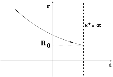
Figure 4.2: The evolution of the surface of the collapsing star for $\lambda=1$ and $\Lambda>0$, given by Eq. (4.2). At the moment $t=t_{0}$, the star collapses to its minimal radius ${\cal{R}}(t_{0})={\cal{R}}_{0}$, at which the extrinsic curvature $K^{+}$ becomes unbounded, while the four-dimensional Ricci scalar remains finite.

$\Lambda<0.$

In this case, substituting the expression for $a(t)$ into (4.85) we obtain

$$I(t)=\sqrt{\frac{|\Lambda|}{3}}\tan\biggl{(}\frac{\sqrt{3|\Lambda|}}{2}(t-t_{0})\biggr{)},$$

and then (4.84) yields

$$\mathcal{R}(t)=\mathcal{R}_{0}\cos^{\frac{2}{3}}\biggl{(}\frac{\sqrt{3|\Lambda|}}{2}(t-t_{0})\biggr{)},$$ (4.98)

where $\mathcal{R}_{0}$ is another constant. Condition (4.72) now implies that $A^{-}_{,t}=0$, i.e. $A^{-}(t)=A_{0}$ for some constant $A_{0}$. Then, by (4.68), $A^{+}(\mathcal{R}(t))=A_{0}$. That is, $A^{+}(r)=A_{0}$ for all $r$ such that $r=\mathcal{R}(t)$ for some $t$. We will assume that $A^{+}=A_{0}$ for all $(t,r)$ in the exterior region, i.e. $A(t,r)=A_{0}.$ Condition (4.66) now implies

$$\rho_{H}^{Im(0)}(t,\mathcal{R}(t))=-\frac{(-6H^{2}+2\Lambda+4\pi G\rho_{H}^{-}(t))\mathcal{R}(t)}{12\pi G}$$

$$=\mathcal{R}_{0}\frac{|\Lambda|-\pi G[1+\cos(\sqrt{3|\Lambda|}(t-t_{0}))]\rho_{H}^{-}(t)}{6\pi G\cos^{\frac{4}{3}}(\frac{\sqrt{3|\Lambda|}}{2}(t-t_{0}))}.$$ (4.99)

Substituting this into condition (4.71), or its equivalent form (4.3.1), we infer that $\rho_{H}^{-}(t)$ satisfies

$$\rho_{H}^{-}(t)=\rho_{H}^{(0)},$$ (4.100)

where $\rho_{H}^{(0)}$ is a constant. All the conditions of Proposition 4.1 are now satisfied, while the condition that $\mu$ be continuous across $\Sigma$ reduces to

$$0 = \frac{2m^{+}}{\mathcal{R}}+\frac{1}{3}\Lambda\mathcal{R}^{2}-2A_{0}+\frac{2}{\mathcal{R}}A_{0}(\mathcal{R}-r_{0})-H^{2}\mathcal{R}^{2}$$

$$= \frac{6m^{+}-6A_{0}r_{0}+\mathcal{R}_{0}^{3}\Lambda}{3\mathcal{R}_{0}\cos^{2/3}(\frac{\sqrt{3|\Lambda|}}{2}(t-t_{0}))}.$$

Thus, the parameter $r_{0}$ is fixed by

$$r_{0}=\frac{6m^{+}+\mathcal{R}_{0}^{3}\Lambda}{6A_{0}}.$$ (4.101)

This implies that

$$\mu^{+}=\frac{1}{2}\ln\biggl{(}\frac{2M}{r}-\frac{|\Lambda|}{3}r^{2}\biggr{)},$$ (4.102)

where $M\equiv|\Lambda|\mathcal{R}_{0}^{3}/6$. Clearly, this corresponds to the Schwarzschild-anti-de Sitter solution. For $\mu^{+}$ to be real, we must assume that $r\leq{\cal{R}}_{0}$. Similar to the last case, the extrinsic curvature $K^{+}$ at $r={\cal{R}}_{0}$ becomes unbounded, while the four-dimensional Ricci scalar ${}^{(4)}R$ remains constant. Thus, in this case it is also not clear whether or not the spacetime is extendible cross $r={\cal{R}}_{0}$.

In any case, all the field equations and junction conditions are now satisfied for $r\leq{\cal{R}}_{0}$, and we have proved the following result.

Proposition 4.3.

Hořava-Lifshitz gravity admits the following explicit solution when $\lambda=1$ and $\Lambda<0$:

$$\mu^{+}=\frac{1}{2}\ln\biggl{(}\frac{|\Lambda|}{3r}(\mathcal{R}_{0}^{3}-r^{3})\biggr{)},\quad\mu^{-}=\ln(-H(t)r),$$

$$\nu=0,\quad H(t)=-\sqrt{\frac{|\Lambda|}{3}}\tan\biggl{(}\frac{\sqrt{3|\Lambda|}}{2}(t-t_{0})\biggr{)},$$

$$\mathcal{R}(t)=\mathcal{R}_{0}\cos^{\frac{2}{3}}\biggl{(}\frac{\sqrt{3|\Lambda|}}{2}(t-t_{0})\biggr{)},$$ (4.103)

$$p_{r}=p_{\theta}=0,\quad\rho_{H}^{-}(t)=\rho_{H}^{(0)},\quad A(t,r)=A_{0},$$

$$\text{$\rho_{H}^{Im(0)}$ is given by (\ref{rhoHIm0dust2})},$$

where $t_{0}$, $\mathcal{R}_{0}$, $A_{0}$, and $\rho_{H}^{(0)}$ are constants.

The evolution of the surface of the collapsing star is illustrated in Fig. 4.3. The collapse starts at an initial time $t_{i}\leq t_{0}$, and at time $t=t_{s}$, the star collapses to a central singularity at which we have $\mathcal{R}(t_{s})=0$, where $t_{s}\equiv t_{0}+\pi/\sqrt{3|\Lambda|}$. Equation (4.99) shows that now both $\rho_{H}^{Im(0)}$ and $\rho_{H}^{-}$ can be positive, provided that $|\Lambda|>2\pi G\rho_{H}^{(0)}.$

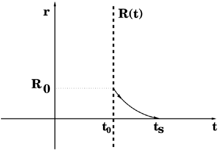
Figure 4.3: The evolution of the surface of the collapsing star for $\lambda=1$ and $\Lambda<0$, given by Eq. (4.3). The star starts to collapse at a time $t=t_{i}\geq t_{0}$. At the later time $t=t_{s}$, at which ${\cal{R}}(t_{s})=0$, the star collapses and a central singularity is formed.

$\Lambda=0.$

In this case, substituting the expression (4.88) for $a(t)$ into (4.85) we obtain

$$I(t)=\frac{2}{3(t_{0}-t)},$$

and then (4.84) yields

$$\mathcal{R}(t)=\mathcal{R}_{0}(t_{0}-t)^{\frac{2}{3}},$$ (4.104)

where $\mathcal{R}_{0}$ is a constant. Condition (4.72) now implies that $A^{-}_{,t}=0$, i.e. $A^{-}(t)=A_{0}$ for some constant $A_{0}$. Then, by (4.68), $A^{+}(\mathcal{R}(t))=A_{0}$. That is, $A^{+}(r)=A_{0}$ for all $r$ such that $r=\mathcal{R}(t)$ for some $t$. Hence (4.104) implies that $A^{+}=A_{0}$ for all $(t,r)$ in the exterior region. Thus, in the present case we also have $A(t,r)=A_{0}.$ Condition (4.66) now implies

$$\rho_{H}^{Im(0)}(t,\mathcal{R}(t))=-\frac{(-6H^{2}+4\pi G\rho_{H}^{-}(t))\mathcal{R}(t)}{12\pi G}$$

$$=\mathcal{R}_{0}\frac{2-3G\pi(t_{0}-t)^{2}\rho_{H}^{-}(t)}{9G\pi(t_{0}-t)^{4/3}}.$$

Substituting this into condition (4.71), or its equivalent form (4.3.1), we infer that

$$\rho_{H}^{-}(t)=\rho_{H}^{(0)},$$ (4.105)

where $\rho_{H}^{(0)}$ is a constant. All the conditions of Proposition 4.1 are now satisfied, and the condition that $\mu$ be continuous across $\Sigma$ becomes

$$0 = \frac{2m^{+}}{\mathcal{R}}-2A_{0}+\frac{2}{\mathcal{R}}A_{0}(\mathcal{R}-r_{0})-H^{2}\mathcal{R}^{2}$$

$$= 2\frac{9m^{+}-9A_{0}r_{0}-2\mathcal{R}_{0}^{3}}{9\mathcal{R}(t)}.$$

Hence, the parameter $r_{0}$ is fixed to

$$r_{0}=\frac{9m^{+}-2\mathcal{R}_{0}^{3}}{9A_{0}},$$ (4.106)

which implies that

$$\mu^{+}=\frac{1}{2}\ln\biggl{(}\frac{r_{g}}{r}\biggr{)},\;\;\nu^{+}=0,\;\;N^{+}=1,$$ (4.107)

where $r_{g}\equiv 4\mathcal{R}_{0}^{3}/9$. This is nothing but is the Schwarzschild solution written in the Painlevé-Gullstrand coordinates [97]. All the field equations and junction conditions are satisfied, so we have proved the following result.

Proposition 4.4.

Hořava-Lifshitz gravity admits the following explicit solution when $\lambda=1$ and $\Lambda=0$:

$$\mu^{+}=\frac{1}{2}\ln\biggl{(}\frac{r_{g}}{r}\biggr{)},\quad\mu^{-}=\ln\big{(}-H(t)r\big{)},$$

$$\nu=0,\quad H(t)=-\frac{2}{3(t_{0}-t)},$$

$$\mathcal{R}(t)=\mathcal{R}_{0}(t_{0}-t)^{\frac{2}{3}},$$ (4.108)

$$p_{r}=p_{\theta}=0,\quad\rho_{H}^{-}(t)=\rho_{H}^{(0)},\quad A(t,r)=A_{0},$$

$$\rho_{H}^{Im(0)}=\mathcal{R}_{0}\frac{2-3G\pi(t_{0}-t)^{2}\rho_{H}^{(0)}}{9G\pi(t_{0}-t)^{4/3}},$$

where $t_{0}$, $\mathcal{R}_{0}$, $A_{0}$, and $\rho_{H}^{(0)}$ are constants.

The evolution of the surface of the collapsing star is shown in Fig. 4.4. The star begins to collapse at the moment $t_{i}$ with a radius $\mathcal{R}_{i}[\equiv\mathcal{R}(t_{i})]$ until the moment $t=t_{0}$, at which we have ${\cal{R}}(t_{0})=0$ and a central singularity is formed. The spacetime outside of the star is given by the Schwarzschild solution. Thus, as in GR, the Schwarzschild spacetime can be formed by the collapse of a homogeneous and isotropic dust perfect fluid [108]. We note that $\rho_{H}^{Im(0)}>0$ for

$$t_{0}-\sqrt{\frac{2}{3G\pi\rho_{H}^{(0)}}}<t<t_{0}.$$

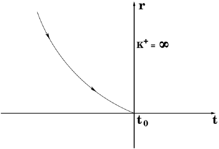
Figure 4.4: The evolution of the surface of the collapsing star for $\lambda=1$ and $\Lambda=0$, given by Eq. (4.4). At the moment $t=t_{i}\leq t_{0}$, the star starts to collapse until the moment $t=t_{0}$, at which we have ${\cal{R}}(t_{0})=0$, whereby a central singularity is formed.

4.3.3 Gravitational Collapse with $\lambda\not=1$

We now consider the case of $\lambda\neq 1$. For an exterior static spherically symmetric vacuum spacetime with $\lambda\neq 1$ and $\Lambda_{g}=0$, equation (4.7) implies that

$$\nu^{+}=-\frac{1}{2}\ln\biggl{(}1-\frac{2B}{r}\biggr{)},$$ (4.109)

where $B$ is a constant. On the other hand, for the interior FLRW region, we have

$$\nu^{-}=-\frac{1}{2}\ln\biggl{(}1-k\frac{r^{2}}{a^{2}(t)}\biggr{)}.$$ (4.110)

Hence, the condition $\nu_{,t}^{+}=\nu_{,t}^{-}$ on $\Sigma$ implies that $0=k\mathcal{R}(t)^{2}.$ Consequently, in order for a solution with $\mathcal{R}(t)\neq 0$ to exist, we must have $k=0$. The conditions that $\nu$ and $\nu_{,r}$ be continuous across $\Sigma$ then reduce to ${2B}/{\mathcal{R}(t)}=0$. Thus, in order for a nontrivial solution to exist we must have $k=B=0$. Thus, we have

$$\nu^{-}=\nu^{+}=0,\qquad\mu^{-}=\ln\big{(}{-rH}\big{)}.$$ (4.111)

On the other hand, since $\lambda\neq 1$, the momentum constraint (4.1) yields

$$\mu^{+}(r)=\ln\biggl{(}C_{1}r+\frac{C_{2}}{r^{2}}\biggr{)},$$ (4.112)

where $C_{1}$ and $C_{2}$ are constants. The field equations (4.1)–(4.1) are then satisfied provided that

$$A^{+}(r)=A_{0}^{+}-\frac{3C_{2}^{2}}{8r^{4}}+\frac{3(1-3\lambda)C_{1}^{2}+2\Lambda}{8}r^{2},$$ (4.113)

where $A_{0}^{+}$ is a constant. It is interesting to note that this class of solutions was first found in [81] in the IR limit. However, since the restriction of the spacetime to the leaves $t=$ constant is flat, we have $R_{ij}=0$, and the higher-order derivative terms of $R_{ij}$ vanish identically, so they are also solutions of the full theory. Moreover, since

$$\mu_{,r}^{+}=\frac{C_{1}r^{3}-2C_{2}}{C_{1}r^{4}+C_{2}r},\qquad\mu_{,r}^{-}=\frac{1}{r},$$

we find

$$\hat{\mu}_{,r}=\frac{-3C_{2}}{C_{1}r^{4}+C_{2}r}.$$ (4.114)

Thus, the requirement that $\mu$ is $C^{1}$ implies that $C_{2}=0$. The continuity of $\mu$ then requires that $H(t)=-C_{1}$ is a constant and so

$$a(t)=a_{0}e^{-C_{1}t}.$$

It follows that $\mu$ is smooth across $\Sigma$. Note also that the asymptotical-flatness condition requires $C_{1}=0$. However, in the following we leave the possibility of $C_{1}\neq 0$ open.

We find that

$$\mathcal{L}_{K}^{+}=3C_{1}^{2}(1-3\lambda),\quad\mathcal{L}_{V}^{+}=2\Lambda,\quad\mathcal{L}_{A}^{+}=0,$$

$$v^{+}=0,\quad J_{A}^{+}=0,\quad J_{\varphi}^{+}=0,\quad\rho_{H}^{+}=0.$$ (4.115)

In order for the integral over the exterior region in the Hamiltonian constraint (4.46) to converge, we also need to assume that

$$3C_{1}^{2}(1-3\lambda)+2\Lambda=0.$$ (4.116)

Thus, $A^{+}(r)=A_{0}^{+}$ is a constant and equation (4.61) implies that $p^{-}(t)=0$, that is, the perfect fluid in the interior region consists of dust.

Similar to the case with $\lambda=1$, the interior solution is still of the form (4.60), i.e.

$$J_{A}^{-}=J_{\varphi}^{-}=0,\quad A^{-}=A^{-}(t).$$

In view of (4.56), we have

$$\mathcal{L}_{\varphi}^{-}=0,\qquad\mathcal{L}_{\lambda}^{-}=0,\qquad\mathcal{L}_{K}^{-}=3(1-3\lambda)H^{2},$$

$$\mathcal{L}_{V}^{-}=2\Lambda,\qquad\mathcal{L}_{A}^{-}=0,\qquad v^{-}=0.$$ (4.117)

We assume that the thin shell of matter separating the interior and exterior solutions is such that

$$p_{r}=0,\quad v=0,\quad J_{\varphi}=J_{\varphi}^{Im(0)}\delta(\Phi),$$

$$p_{\theta}=p_{\theta}^{Im(0)}\delta(\Phi),\quad\rho_{H}=\rho_{H}^{-}+\rho_{H}^{Im(0)}\delta(\Phi),\qquad$$

$$A=A^{D}+A^{Im(0)}\delta(\Phi),\quad J_{A}=0,\quad\mathcal{L}_{A}=\mathcal{L}_{A}^{-},$$ (4.118)

with $\rho_{H}^{-}=\rho_{H}^{-}(t)$.

Proposition 4.5.

For the spacetime defined by (4.111)–(4.118), the six junction conditions (4.46)–(4.2.2) reduce to the following six conditions:

$$\rho_{H}^{-}(t)\frac{\mathcal{R}(t)}{3}+\rho_{H}^{Im(0)}(t,\mathcal{R}(t))=0,$$ (4.119)

$$J_{\varphi}^{Im(0)}=0,$$ (4.120)

$$\text{$A(t,r)=A_{0}$ is a constant},$$ (4.121)

$$p_{\theta}^{Im(0)}=0\text{ on $\Sigma$,}$$ (4.122)

$$\frac{d}{dt}\Bigl{[}\rho_{H}^{Im(0)}(t,\mathcal{R}(t))\Bigr{]}+2\frac{\dot{\mathcal{R}}(t)}{\mathcal{R}(t)}\rho_{H}^{Im(0)}(t,\mathcal{R}(t))$$

$$+\dot{\mathcal{R}}(t)\rho_{H}^{-}(t)+\frac{C_{1}\rho_{H,t}^{-}(t)\mathcal{R}(t)^{2}}{4}=0.$$ (4.123)

Proof.  For the spacetime defined by (4.111)–(4.118), condition (4.46) reduces to

$$\left(3(1-3\lambda)C_{1}^{2}+2\Lambda+4\pi G\rho_{H}^{-}(t)\right)\int_{0}^{\mathcal{R}(t)}r^{2}dr$$

$$+\int_{\mathcal{R}(t)}^{\infty}\biggl{(}3C_{1}^{2}(1-3\lambda)+2\Lambda\biggr{)}r^{2}dr$$

$$+4\pi G\rho_{H}^{Im(0)}r^{2}\Big{|}_{r=\mathcal{R}(t)}=0,$$

which, in view of (4.116), yields (4.119). Moreover, equation (4.52) reduces to (4.120).

The functions $F$ and $F^{A}$ are given by (4.75)–(4.76) also for $\lambda\neq 1$. Hence, condition (4.48) implies that $A$ is continuous across $\Sigma$ just like in the case of $\lambda=1$. Since $A^{+}=A_{0}^{+}$ is constant and $A^{-}(t)$ is independent of $r$, this gives (4.121). Condition (4.2.2) then reduces to

$$\frac{1}{r}F_{\theta\theta}^{AIm(0)}\delta(\Phi)+\frac{1}{r}F_{\theta\theta}^{AIm(1)}\delta^{\prime}(\Phi)$$

$$+\frac{1}{r}F_{\theta\theta}^{AIm(2)}\delta^{\prime\prime}(\Phi)+8\pi Grp_{\theta}^{Im(0)}\delta(\Phi)=0.$$

Since $A$ is a constant, this yields (4.122).

Conditions (4.50) and (4.2.2) reduce to (4.123) and (4.122). $\Box$

Conditions (4.119) and (4.123) imply that

$$\dot{\rho}_{H}^{-}(t)\mathcal{R}(t)\bigg{(}\frac{C_{1}}{4}\mathcal{R}(t)-\frac{1}{3}\bigg{)}=0.$$

Excluding the case of no collapse where $\mathcal{R}(t)$ is a constant, it follows that $\rho_{H}^{-}$ must be a constant. If this is the case, then the junction conditions are satisfied provided that $\rho_{H}^{Im(0)}(t,\mathcal{R}(t))=-\rho_{H}^{-}\mathcal{R}(t)/3$.

In summary, in the case $\lambda\not=1$ a static spherical spacetime can be produced by gravitational collapse of a homogeneous and isotropic dust fluid. However, the space-time outside of such a fluid is not asymptotically flat, as one can see from Eqs. (4.111) and (4.112) with $C_{2}=0$.

4.4 Conclusions

In this chapter, we have studied gravitational collapse of a spherical cloud of fluid with a finite radius in the framework of the nonrelativistic general covariant theory of HL gravity with the projectability condition and an arbitrary coupling constant $\lambda$. Using distribution theory, we have developed the general junction conditions for such a collapsing spherical body, under the minimal requirement that the junctions should be mathematically meaningful in the sense of generalized functions. The general junction conditions have been summarized in Table I.

As one of the simplest applications, we have studied a collapsing star that is made of a homogeneous and isotropic perfect fluid, while the external region is described by a stationary spacetime. We have found that the problem reduces to the matching of six independent conditions that the Arnowitt-Deser-Misner variables ($N,N^{i},g_{ij}$) and the gauge field $A$ and Newtonian prepotential $\varphi$ must satisfy.

For the case of a homogeneous and isotropic dust fluid (a perfect fluid with vanishing pressure), we have found explicitly the space-time outside of the collapsing sphere. In particular, in the case $\lambda=1$, the external spacetimes are described by the Schwarzschild (anti-) de Sitter solutions, written in Painlevé-Gullstrand coordinates [97]. It is remarkable that the collapse of a homogeneous and isotropic dust to a Schwarzschild black hole, studied by Oppenheimer and Snyder in General Relativity more than 80 years ago [110], is a particular case. However, there are fundamental differences. First, in General Relativity a thin shell does not necessarily appear on the surface of the collapsing sphere [110], while in the current case we have shown that such a thin shell must exist, in General Relativity, because of the local conservation of energy of the collapsing body, the energy density of the dust fluid is inversely proportional to the cube of the radius of the fluid, while in the current case it remains a constant, as the conservation law is global [cf. Eq. (2.15)] and the energy of the collapsing star is not necessarily conserved locally.

In the case $\lambda\not=1$, the space-time outside of the homogeneous and isotropic dust fluid is described by Eqs. (4.111) and (4.112) with $C_{2}=0$. It is clear that such a space-time is not asymptotically flat. Therefore, in this case to obtain an asymptotically flat space-time outside of a collapsing dust fluid, it must not be homogeneous and/or isotropic.

From the above simple examples, one can already see the significant differences between the HL theory and General Relativity in the strong gravitational field regime. Therefore, it is very interesting to study gravitational collapse of more general fluids, such as perfect fluids with different equations of state, or anisotropic fluids with or without heat flows. Particular attention should be paid to the roles that the equation of state and heat flows might play. It would be extremely interesting to study the implications for black hole physics, or more generally for (observational) astrophysics and cosmology [108]. Since the general formulas have been already laid down in this chapter, we expect that such studies can be carried out easily.

As emphasized previously, our treatment of the junction conditions of a collapsing star presented in this chapter can be easily generalized to other versions of Hořava-Lifshitz gravity or, more generally, to any model of a higher-order derivative gravity theory.

Chapter 5 Global Structure of Spacetime

This chapter published as: J. Greenwald, J. Lenells, J. X. Lu, V. H. Satheeshkumar and A. Wang, “Black holes and global structures of spherical spacetimes in Hořava-Lifshitz Theory,” Phys. Rev. D 84, 084040 (2011).

5.1 Introduction

In the HL theory, due to the breaking of the general covariance, the dispersion relations of particles usually contain high order momentum terms [123, 124, 125, 126, 127],

$$\omega_{k}^{2}=m^{2}+k^{2}\left(1+\sum^{z-1}_{n=1}{\lambda_{n}\left(\frac{k}{M_{n}}\right)^{2n}}\right),$$ (5.1)

for which the group velocity is given by [128]

$$v_{k}=\frac{k}{\omega}\left(1+\sum^{z-1}_{n=1}{(n+1)\lambda_{n}\left(\frac{k}{M_{n}}\right)^{2n}}\right).$$ (5.2)

As an immediate result, the speed of light becomes unbounded in the UV. This makes the causal structure of the spacetimes quite different from that given in GR, where the light cone of a given point $p$ plays a fundamental role in determining the causal relationship of $p$ to other events [cf. Fig. 5.1]. However, once the general covariance is broken, the causal structure will be dramatically changed. For example, in the Newtonian theory, time is absolute and the speeds of signals are not limited. Then, the causal structure of a given point $p$ is uniquely determined by the time difference, $\Delta{t}\equiv t_{p}-t_{q}$, between the two events. In particular, if $\Delta{t}>0$, the event $q$ is to the past of $p$; if $\Delta{t}<0$, it is to the future; and if $\Delta{t}=0$, the two events are simultaneous.

Figure 5.1: (a) The light cone of the event $p$ in special relativity. (b) The causal structure of the point $p$ in Newtonian theory.

Another consequence of the breaking of the general covariance is that free particles now do not follow geodesics. This immediately makes all the definitions of black holes given in General Relativity invalid [129, 130, 131, 132]. To provide a proper definition of black holes, anisotropic conformal boundaries [133] and kinematics of particles  [134] have been studied within the HL framework. In this chapter, we shall adopt the approach of Kiritsis and Kofinas (KK) [135], where a horizon is defined as the infinitely redshifted 2-dimensional (closed) surface of massless test particles. Clearly, such a definition reduces to that given in General Relativity when the dispersion relation is relativistic [Where $\lambda_{n}=0$, as shown in Eq. (5.1).].

It should be noted that black holes in the HL theory with or without the projectability condition have been extensively studied, mainly using the definition borrowed directly from GR. In this chapter, we shall show explicitly how these definitions are changed by considering some particular examples, found in the HMT set up with $\lambda=1$.

Another interesting approach is the equivalence between the HL theory (without the projectability condition) and the Einstein-aether theory in the IR  [136], where the former is equivalent to the latter for the case where the aether vector field $u_{\mu}$ is hypersurface-orthogonal. In the spherically symmetric case, this is not a restriction as the aether field $u_{\mu}$ now is always hypersurface-orthogonal. From such studies one already sees the difficulties to define black holes, because of the fact that different modes may have different velocities even in the IR. In [136], black holes are defined to possess both a metric horizon and a spin-0 mode horizon. Since the equivalence holds only in the IR, it is still unclear how to extend such definitions to high energy scales, where high order curvature terms become important.

5.2 Black Holes in HL Theory

Kristis and Kofinas (KK) considered a scalar field with a given dispersion relation $F(\zeta)$  [135]. In the geometrical optical approximations, $\zeta$ is given by $\zeta=g_{ij}k^{i}k^{j}$, where $k_{i}$ denotes the 3-momentum of the corresponding spin-0 particle. With this approximation, the trajectory of a test particle is given by

$$S_{p} \equiv \int_{0}^{1}{{\cal{L}}_{p}d\tau}$$ (5.3)

$$= \frac{1}{2}\int_{0}^{1}{d\tau\Bigg{\{}\frac{c^{2}N^{2}}{e}\dot{t}^{2}+e\Big{[}F(\zeta)-2\zeta F^{\prime}(\zeta)\Big{]}\Bigg{\}}},~{}~{}~{}~{}$$

where $e$ is a one-dimensional einbein, and $\zeta$ is now considered as a functional of $t,x^{i},\dot{t},\dot{x}^{i}$ and $e$, given by the relation,

$$\zeta\;[F^{\prime}(\zeta)]^{2}=\frac{1}{e^{2}}g_{ij}\big{(}\dot{x}^{i}+N^{i}\dot{t}\big{)}\big{(}\dot{x}^{j}+N^{j}\dot{t}\big{)},$$ (5.4)

with $\dot{t}\equiv dt/d\tau$, etc. For detail, we refer readers to [135].

It should be noted that KK obtained the above action starting from a scalar field. So, strictly speaking, it is valid only for spin-0 test particles. However, what is really important in their derivations is the dispersion relationship $F(\zeta)$. As shown in [137], a spin-2 particle has a similar dispersion relation. It is expected that a spin-1 test particle, such as photons, should have a similar dispersion relation too [128, 135]. Therefore, in the rest of this chapter and without proof, we simply consider the action (5.3) to describe all massless test particles.

Spherically symmetric static spacetimes in the framework of the HMT setup were studied systematically in [79, 78], and the metric for static spherically symmetric spacetimes that preserve the form of Eq. (2.2) with the projectability condition can be cast in the form [103] given below. Note the slight difference between the $g_{tr}$ term defined here and the one defined in [103, 78].

$$ds^{2}=-c^{2}dt^{2}+e^{2\nu}\left(dr+e^{\mu-\nu}cdt\right)^{2}+r^{2}d^{2}\Omega,$$ (5.5)

where $d^{2}\Omega=d\theta^{2}+\sin^{2}\theta d\phi^{2}$, and

$$\mu=\mu(r),\;\;\;\nu=\nu(r),\;\;\;N^{i}=\left\{ce^{\mu-\nu},0,0\right\}.$$ (5.6)

The corresponding timelike Killing vector is $\xi=\partial_{t}$, and the diagonal case $N^{r}=0$ corresponds to $\mu=-\infty$.

However, to study black hole solutions in a more general case, in this (and only in this) section, we also consider the case without projectability condition, and write the metric as,

$$ds^{2}=-N^{2}c^{2}dt^{2}+\frac{1}{f}\left(dr+N^{r}cdt\right)^{2}+r^{2}d^{2}\Omega.$$ (5.7)

where $N,\;f$ and $N^{r}$ are all functions of $r$. Without loss of generality, in the rest of the chapter we shall set $c=1$, which is equivalent to the coordinate transformations $x_{0}=ct,\;\bar{N}^{r}=N^{r}/c$. Taking

$$F(\zeta)=\zeta^{n},\;(n=1,2,...),$$ (5.8)

Eq. (5.4) yields,

$$\zeta=\left(\frac{\dot{r}+N^{r}\dot{t}}{ne\sqrt{f}}\right)^{{2}/{(2n-1)}}\equiv\left(\frac{{\cal{D}}}{e^{2}}\right)^{{1}/{(2n-1)}}.$$ (5.9)

Inserting this into Eq. (5.3), we find that, for radially moving particles, ${\cal{L}}_{p}$ is given by

$${\cal{L}}_{p}=\frac{N^{2}}{2e}\dot{t}^{2}+\frac{1}{2}\big{(}1-2n\big{)}e^{1/(1-2n)}{\cal{D}}^{{n}/{(2n-1)}}.$$ (5.10)

Then, from the equation $\delta{\cal{L}}_{p}/\delta{e}=0$ we obtain

$$N^{2}\dot{t}^{2}-e^{2(n-1)/(2n-1)}{\cal{D}}^{{n}/{(2n-1)}}=0.$$ (5.11)

On the other hand, since $\delta{\cal{L}}_{p}/\delta{t}=0$, the Euler-Lagrange equation,

$$\frac{\delta{\cal{L}}_{p}}{\delta{t}}-\frac{1}{d\tau}\left(\frac{\delta{\cal{L}}_{p}}{\delta{\dot{t}}}\right)=0,$$

yields

$$N^{2}\dot{t}-e^{2(n-1)/(2n-1)}\frac{N^{r}}{\sqrt{f}}{\cal{D}}^{{1}/{[2(2n-1)]}}=eE,$$ (5.12)

where $E$ is an integration constant, representing the total energy of the test particle.

To solve Eqs. (5.11) and (5.12), we first consider the case $n=1$, which corresponds to the relativistic dispersion relation. From such considerations, we shall see how to generalize the definition of black holes given in General Relativity to the HL theory where $n$ is generically different from 1, as required by the renormalizability condition in the UV.

5.2.1 $n=1$

In this case, Eqs. (5.11) and (5.12) reduce, respectively, to,

$$N^{2}\dot{t}^{2}-{\cal{D}} = 0,$$ (5.13)

$$N^{2}\dot{t}-{N^{r}}\sqrt{\frac{\cal{D}}{f}} = eE.$$ (5.14)

Eq. (5.13) simply tells us that now the particle moves along null geodesics. The above equations can be easily solved according to whether $N^{r}$ vanishes or not.

$N^{r}=0.$

When $N^{r}=0$, from Eq. (5.13) we find

$$dt=\pm\frac{dr}{N\sqrt{f}},$$ (5.15)

where “+” (“$-$”) corresponds to out-going (in-going) light rays. If $f$ has an a-th order zero and $N^{2}$ a b-th order zero at a surface, say, $r=r_{g}$, that is,

$$f=f_{0}(r)(r-r_{g})^{a},\;\;\;N=N_{0}(r)(r-r_{g})^{b/2},$$ (5.16)

where $N_{0}(r_{g})\not=0$ and $f_{0}(r_{g})\not=0$, then from the above equations we find that in the neighborhood of $r=r_{g}$,

$$t\simeq t_{0}\pm\frac{1}{N_{0}\sqrt{f_{0}}}\begin{cases}\frac{2}{2-(a+b)}(r-r_{g})^{1-(a+b)/2},&a+b\not=2,\\ \ln\left|r-r_{g}\right|,&a+b=2.\\ \end{cases}$$ (5.17)

Therefore, when

$$a+b\geq 2,\;(n=1),$$ (5.18)

$t$ becomes unbounded, as $r\rightarrow r_{g}$, at which the light rays are infinitely redshifted. This indicates that an event horizon might exist at $r=r_{g}$, provided that the spacetime has no curvature singularity there. A simple example is the Schwarzschild solution, $N^{2}=f=(r-r_{g})/r$, which is also a solution of the HL theory without the projectability condition, but with the detailed balance condition softly broken [138], and for which we have $a=b=1$. Clearly, it satisfies the above condition with the equality, so $r=r_{g}$ indeed defines a horizon.

$N^{r}\not=0.$

When $N^{r}\not=0$, Eq. (5.13) yields

$$t=t_{0}+\int{\frac{\epsilon dr}{N\sqrt{f}-\epsilon N^{r}}},$$ (5.19)

where $\epsilon=+1\;(\epsilon=-1)$ corresponds to out-going (in-going) light rays. If

$$H(r)\equiv N\sqrt{f}-\epsilon N^{r},$$ (5.20)

has $\delta$-th order zero at $r_{g}$,

$$H(r)=H_{0}(r)(r-r_{g})^{\delta},$$ (5.21)

with $H_{0}(r_{g})\not=0$, we find that in the neighborhood $r=r_{g}$ Eq. (5.19) yields

$$t=t_{0}+\frac{\epsilon}{H_{0}(r_{g})}\begin{cases}\frac{1}{1-\delta}(r-r_{g})^{1-\delta},&\delta\not=1,\\ \ln(r-r_{g}),&\delta=1.\\ \end{cases}$$ (5.22)

Clearly, when

$$\delta\geq 1,(n=1),$$ (5.23)

$|t|$ becomes unbounded as $r\rightarrow r_{g}$, and an event horizon might exist.

The Schwarzschild solution in the Painlevé-Gullstrand coordinates  [97] is given by

$$N_{Sch}^{2}=f_{Sch}=1,\;\;\;N_{Sch}^{r}=\epsilon_{1}\sqrt{\frac{r_{g}}{r}},$$ (5.24)

where $\epsilon_{1}=\pm 1$. As shown in [79, 78], this is also a vacuum solution of the HL theory in the HMT setup [73]. Then, we find that $H(r)=1-\epsilon_{1}\epsilon\sqrt{r_{g}/r}$. Thus, for the solution with $\epsilon_{1}=+1$, the time of the out-going null rays, measured by asymptotically flat observers, becomes unbounded at $r_{g}$, and for the solution with $\epsilon_{1}=-1$, the time of the in-going null rays becomes unbounded. Therefore, an event horizon is indicated to exist at $r=r_{g}$ in both cases.

In review of the above, KK generalized the notion of black holes defined in General Relativity to the case of a non-standard dispersion relation [135]. In summary, a horizon is defined as a surface on which light rays are infinitely redshifted. It should be noted that this redshift should be understood as measured by asymptotically flat observers at $N(r\gg r_{g})\simeq 1$ and $N^{r}(r\gg r_{g})\simeq 0$, with $r$ being the geometric radius, $r=\sqrt{A/4\pi}$, of the 2-sphere: $t,r=$ constants, where $A$ denotes the area of the 2-sphere.

5.2.2 $n\geq 2$

In this case, eliminating $e$ from Eqs. (5.11) and (5.12) we find that

$$X^{n}-p(r)X-q(r,E)=0,$$ (5.25)

where

$$X \equiv \left(\frac{\sqrt{\cal{D}}}{\dot{t}}\right)^{1/(n-1)}=\left(\frac{\left|r^{\prime}+N^{r}\right|}{n\sqrt{f}}\right)^{1/(n-1)},$$

$$p(r) \equiv \frac{N^{r}}{\sqrt{f}},\;\;\;q(r,E)\equiv EN^{1/(n-1)},$$ (5.26)

with $r^{\prime}\equiv\dot{r}/\dot{t}=dr/dt$. To solve the above equation, again it is found convenient to consider the cases $N^{r}=0$ and $N^{r}\not=0$ separately.

$N^{r}=0.$

When $N^{r}=0$, Eq. (5.25) has the solution,

$$t=t_{0}+\epsilon\int{\frac{dr}{nE^{(n-1)/n}\sqrt{f}N^{1/n}}},$$ (5.27)

where $\epsilon=+1$ corresponds to outgoing rays, and $\epsilon=-1$ to ingoing rays. Thus, if $f$ has an a-th order zero and $N^{2}$ a b-th order zero at $r=r_{g}$, as given by Eq. (5.16), we have $\sqrt{f}N^{1/n}\sim(r-r_{g})^{(a+b/n)/2}$. Then, from the above, we find that the time $t$, measured by asymptotically flat observers, becomes infinitely large at $r=r_{g}$, provided that  [135]

$$a+\frac{b}{n}\geq 2.$$ (5.28)

For the solutions with the projectability condition ($N=1,\;b=0$), this is possible only when $a\geq 2$.

Considering again the Schwarzschild solution, $N^{2}=f=(r-r_{g})/r$, one finds that this does not satisfy the condition (5.28) with $n\geq 2$. Therefore, the Schwarzschild black hole in General Relativity is no longer a black hole in the HL theory, because of the non-relativistic dispersion relations (5.1). This is expected, since even in General Relativity when quantum effects are taken into account, such as the Hawking radiation, classical black holes are no longer black.

$N^{r}\not=0.$

In this case, let us consider an ingoing ray ${r}^{\prime}<0$. Suppose there is a horizon located at $r=r_{H}$. Then $r^{\prime}(r)\simeq 0$ as we approach the horizon. Thus, if $N^{r}>0$ and bounded away from zero, $(r^{\prime}+N^{r})$ will also be positive, when the ray is sufficiently near the horizon. Conversely, if $N^{r}<0$ and bounded away from zero, then $(r^{\prime}+N^{r})$ will be negative sufficiently near the horizon. Defining $H$ by $H(r,E)\equiv r^{\prime}$, we find that for an ingoing ray near the horizon we have,

$$t=t_{0}+\int\frac{dr}{H(r,E)},$$ (5.29)

$$H(r,E)=\epsilon n\sqrt{f}X^{n-1}-N^{r},$$ (5.30)

where

$$\epsilon=\begin{cases}1,&N^{r}>0,\\ -1,&N^{r}<0.\\ \end{cases}$$ (5.31)

Dividing (5.25) by $X$ and solving for $X^{n-1}$, we obtain

$$X^{n-1}=\frac{N^{r}}{\sqrt{f}}+\frac{EN^{\frac{1}{n-1}}}{X}.$$

Substituting this into (5.30), we find,

$$H=(\epsilon n-1)N^{r}+\epsilon n\sqrt{f}\frac{EN^{\frac{1}{n-1}}}{X}.$$ (5.32)

It follows that if $H$ has a zero at $r=r_{H}$, then

$$X|_{r=r_{H}}=-\frac{\epsilon n\sqrt{f}EN^{\frac{1}{n-1}}}{(\epsilon n-1)N^{r}}.$$ (5.33)

The expression on the rhs is positive (negative) for $\epsilon=-1$ ($\epsilon=1$). Thus, $H$ can have a zero only if $\epsilon=-1$. Thus, we will henceforth consider only this case. Differentiation of (5.32) with respect to $r$ yields

$$H^{\prime}(r)=-(n+1)N^{r^{\prime}}-n\sqrt{f}\frac{EN^{\frac{1}{n-1}-1}}{(n-1)X}N^{\prime}-n\frac{EN^{\frac{1}{n-1}}}{2\sqrt{f}X}f^{\prime}+n\sqrt{f}\frac{EN^{\frac{1}{n-1}}}{X^{2}}X^{\prime}.~{}~{}~{}~{}$$ (5.34)

On the other hand, differentiation of (5.25) with respect to $r$ yields

$$X^{\prime}(r)=\frac{1}{nX^{n-1}-\frac{N^{r}}{\sqrt{f}}}\left[\left(\frac{1}{\sqrt{f}}\frac{dN^{r}}{dr}-\frac{N^{r}}{2f^{3/2}}\frac{df}{dr}\right)X+\frac{EN^{\frac{1}{n-1}-1}}{n-1}\frac{dN}{dr}\right].$$ (5.35)

Substituting the above into Eq. (5.34), we find that

$$H^{\prime}(r)\bigg{|}_{r=r_{H}}=-\frac{n+1}{2}\Biggl{(}\frac{H_{1}}{H_{2}}-\frac{N^{r}f^{\prime}}{f}+\frac{2N^{r}N^{\prime}}{N-nN}+2N^{r^{\prime}}\Biggr{)},$$ (5.36)

where

$$H_{1}\equiv 2E(n+1)fN^{r}N^{\prime}+E(n-1)nN\left(N^{r}f^{\prime}-2fN^{r^{\prime}}\right),$$

$$H_{2}\equiv(n-1)nfN\Bigg{[}E+(n+1)N^{\frac{1}{1-n}}\left(\frac{En\sqrt{f}N^{\frac{1}{n-1}}}{(-n-1)N^{r}}\right)^{n}\Bigg{]}.$$ (5.37)

If $H$ has a zero of order $\delta>0$ at $r_{H}$, we can write it in the form,

$$H(r)=H_{0}(r_{H})(r-r_{H})^{\delta}+\cdots,$$ (5.38)

as $r\to r_{H}$, where $H_{0}(r_{H})\neq 0$. Therefore,

$$H^{\prime}(r)\bigg{|}_{r=r_{H}}=\begin{cases}0,&\delta>1,\\ H_{0}(r_{H}),&\delta=1,\\ \pm\infty,&0<\delta<1.\end{cases}$$ (5.39)

Now $t\to\infty$ as $r\rightarrow r_{H}^{+}$ if and only if

$$\delta\geq 1,$$ (5.40)

which happens if and only if ${dH}/{dr}\big{|}_{r=r_{H}}$ is finite. This gives an explicit condition on $f,N,N^{r},E,n$ for the blow-up of $t$ at $r_{H}$.

It should be noted that $r_{H}$ usually depends on the energy $E$ of the test particles, as can be seen from the above and specific examples considered below.

Case $n=2$: In this case, we have

$$H^{\prime}(r)\bigg{|}_{r=r_{H}}=\frac{H_{3}}{2N\left[4EfN+3(N^{r})^{2}\right]},$$ (5.41)

where

$$H_{3}\equiv 3\left[4EN^{2}\left(N^{r}f^{\prime}-2fN^{r^{\prime}}\right)+8EfNN^{r}N^{\prime}\right.-3(N^{r})^{3}N^{\prime}\Big{]},(n=2).$$ (5.42)

Again, for the Schwarzschild solution (5.24), we have

$$X(r) = \frac{1}{2}\left(-\sqrt{\frac{r_{g}}{r}}+\frac{\sqrt{4Er+r_{g}}}{\sqrt{r}}\right),$$

$$H(r) = \frac{-3\sqrt{r_{g}(4Er+r_{g})}+4Er+3r_{g}}{\sqrt{rr_{g}}-\sqrt{r(4Er+r_{g})}},$$ (5.43)

so that $H(r)=0$ has the solution,

$$r_{H}=\frac{3r_{g}}{4E},\;(n=2),$$ (5.44)

at which we have

$$H^{\prime}(r_{H})=-\frac{2E^{3/2}}{\sqrt{3}r_{g}}.$$ (5.45)

Then, according to Eq. (5.39), we have $\delta=1$, i.e., $t$ diverges logarithmically as $r\rightarrow r_{H}^{+}$. Therefore, in this case there does exist a horizon. But, the location of it depends on the energy $E$ of the test particle, and approaches zero when $E\gg r_{g}$. This is understandable, as the speed of light is unbounded in the UV, and in principle the singularity located at $r=0$ can be seen by asymptotically flat observers, as long as the light rays sent by the observers have sufficiently high energies.

Case $n=3$: In this case, we have

$$X^{3}-p(r)X-q(r,E)=0.$$ (5.46)

Assuming that $H(r)=0$ has a real and positive root $r_{H}$, we find that

$$H^{\prime}(r)\bigg{|}_{r=r_{H}}=\frac{H_{4}}{3N\left(27E^{2}f^{3/2}N-16(N^{r})^{3}\right)},$$ (5.47)

where

$$H_{4}\equiv 162E^{2}\sqrt{f}N^{2}N^{r}f^{\prime}+32(N^{r})^{4}N^{\prime}-162E^{2}f^{3/2}N\left(2NN^{r^{\prime}}-N^{r}N^{\prime}\right).$$ (5.48)

For the Schwarzschild solution (5.24), we have $p(r)=-\sqrt{r_{g}/r}$ and $q(r,E)=E$. Then, we find that

$$X^{3}+\sqrt{\frac{r_{g}}{r}}X-E=0,$$ (5.49)

$$H(r)=4\sqrt{\frac{r_{g}}{r}}-\frac{3E}{X},$$ (5.50)

from which we find that $H(r)=0$ has a solution,

$$r_{H}=r_{g}\left(\frac{16}{27E^{2}}\right)^{2/3},\;(n=3),$$ (5.51)

which also depends on $E$, and approaches zero as $E\rightarrow\infty$. Substituting $r_{H}$ into Eq. (5.47), we find $H^{\prime}(r_{H})=-27E^{2}/(16r_{g})$. That is, the hypersurface $r=r_{H}$ is also an observer-dependent horizon in the case $n=3$, and the radius of the horizon is inversely proportional to the energy of the test particle. For $E\gg r_{g}$, we have $r_{H}\simeq 0$.

Another (simpler) consideration for the existence of the horizon is given as follows: First, from Eq. (5.2.2) we find that

$$X=\left(\frac{|r^{\prime}+N^{r}|}{n\sqrt{f}}\right)^{1/(n-1)}\simeq\left(\frac{\epsilon N^{r}}{n\sqrt{f}}\right)^{1/(n-1)}\times\left(1+\frac{H}{(n-1)N^{r}}\right),$$ (5.52)

for $r\simeq r_{H}$. Inserting it into Eq. (5.32), we have, to leading order,

$$\left(1+\frac{EN^{1/(n-1)}}{(n-1)\left(\frac{\epsilon N^{r}}{n\sqrt{f}}\right)^{n/(n-1)}}\right)H(r,E)=(\epsilon n-1)N^{r}\left(1+\frac{EN^{1/(n-1)}}{(\epsilon n-1)\left(\frac{\epsilon N^{r}}{n\sqrt{f}}\right)^{n/(n-1)}}\right).$$ (5.53)

Then, we obtain

$$\left.\frac{EN^{1/(n-1)}}{(n+1)\left(\frac{-N^{r}}{n\sqrt{f}}\right)^{n/(n-1)}}\right|_{r=r_{H}}=1.$$ (5.54)

Given this, we can further simplify Eq. (5.53) to,

$$\frac{2n}{n-1}H(r,E)=-(n+1)N^{r}(r_{H})\left(1-\frac{EN^{1/(n-1)}(r)}{(n+1)\left(\frac{-N^{r}(r)}{n\sqrt{f(r)}}\right)^{n/(n-1)}}\right).~{}~{}~{}~{}~{}~{}~{}~{}~{}~{}$$ (5.55)

Then, using Eq. (5.38), we have the following constraint for $N,N^{r},f$ to satisfy so that a horizon can indeed exist,

$$\frac{EN^{1/(n-1)}(r)}{(n+1)\left(\frac{-N^{r}(r)}{n\sqrt{f(r)}}\right)^{n/(n-1)}}=1+\frac{2nH_{0}(r_{H})}{(n^{2}-1)N^{r}(r_{H})}(r-r_{H})^{\delta}+\cdots.~{}~{}~{}~{}~{}~{}~{}~{}$$ (5.56)

This equation can be first used to determine $r_{H}$ and then $\delta$, once $N,\;N^{r}$ and $f$ are given. To illustrate how to use it, let us consider the Schwarzschild metric (5.24). For $n=2$, $r_{H}$ can be obtained simply from the above, and is given exactly by Eq. (5.44), for which we have

$$\frac{EN^{1/(n-1)}(r)}{(n+1)\left(\frac{-N^{r}(r)}{n\sqrt{f(r)}}\right)^{n/(n-1)}}\simeq 1+\frac{r-r_{H}}{r_{H}},~{}~{}~{}~{}~{}$$ (5.57)

that is, $\delta=1$.

For $n=3$, from Eq. (5.54) we find that $r_{H}$ is given by Eq. (5.51), and

$$\frac{EN^{1/(n-1)}(r)}{(n+1)\left(\frac{-N^{r}(r)}{n\sqrt{f(r)}}\right)^{n/(n-1)}}=\frac{3^{3/2}Er^{3/4}}{4r_{g}^{3/4}}\simeq 1+\frac{3}{4r_{H}}(r-r_{H})+\cdots.$$ (5.58)

Therefore, in this case we have $\delta=1$ too.

It should be noted that in the above analysis, we assumed that $F(\zeta)=\zeta^{n}$. In more realistic models, the dispersion relation is a polynomial of $\zeta$, as shown by Eq. (5.1), or more specifically,

$$F(\zeta)=\zeta+\frac{\zeta^{2}}{M^{2}_{A}}+\frac{\zeta^{4}}{M^{4}_{B}}+...,$$ (5.59)

where $M_{A}$ and $M_{B}$ are the energy scales, which can be significantly different from the Planck one [139]. Therefore, for observers in low energy scales, where $\zeta\ll M_{A},M_{B}$, the first term dominates, and some solutions, including the Schwarzschild solution, look like black holes, as shown in the case $n=1$. But, for observers with high energies, those solutions may not be black holes any longer. Even if they are, their horizons in general are observer-dependent, as shown in the cases $n=2$ and $n=3$ explicitly for the Schwarzschild solution. To illustrate the main properties of the dispersion relation (5.59), we shall consider the case where only the first two terms are important.

5.2.3 Trajectories of Test Particles with the Dispersion Relation $F(\zeta)=\zeta+{\zeta^{2}}/{M^{2}_{A}}$

For the sake of simplicity, we restrict ourselves to the case $N^{r}=0$. Substituting

$$F(\zeta)=\zeta+\frac{\zeta^{2}}{M^{2}_{A}},$$ (5.60)

into Eq. (5.4), we find

$$\zeta\left(1+\frac{2\zeta}{M_{A}^{2}}\right)^{2}=\frac{\dot{r}^{2}}{e^{2}f}.$$ (5.61)

Solving this equation directly for $\zeta$ yields a very complicated expression, and it is not clear how to proceed along this direction. Instead, we note that our goal is to find the analog of equation (5.11), i.e. of the equation $\delta\mathcal{L}_{p}/\delta e=0$, where

$$\mathcal{L}_{p} = \frac{1}{2}\left(\frac{N^{2}}{e}\dot{t}^{2}+e\Big{[}F(\zeta)-2\zeta F^{\prime}(\zeta)\Big{]}\right)$$ (5.62)

$$= \frac{1}{2}\left(\frac{N^{2}}{e}\dot{t}^{2}-e\left[\zeta+\frac{3\zeta^{2}}{M_{A}^{2}}\right]\right).$$

Thus, we will first calculate $\delta\zeta/\delta e$, implicitly by applying $\delta/\delta e$ to both sides of (5.61), which yields,

$$\frac{\delta\zeta}{\delta e}=-\frac{2M_{A}^{4}\dot{r}^{2}}{e^{3}f(M_{A}^{4}+8M_{A}^{2}\zeta+12\zeta^{2})}.$$ (5.63)

Substituting this into the expression

$$\frac{\delta\mathcal{L}_{p}}{\delta e}=\frac{1}{2}\left(-\frac{N^{2}}{e^{2}}\dot{t}^{2}-\left[\zeta+\frac{3\zeta^{2}}{M_{A}^{2}}\right]-e\left[\frac{\delta\zeta}{\delta e}+\frac{6\zeta}{M_{A}^{2}}\frac{\delta\zeta}{\delta e}\right]\right),$$

we find the following analog of equation (5.11),

$$\zeta\left(e^{2}M_{A}^{2}+2N^{2}\dot{t}^{2}\right)+5e^{2}\zeta^{2}+\frac{6e^{2}\zeta^{3}}{M_{A}^{2}}+M_{A}^{2}\left(N^{2}\dot{t}^{2}-\frac{2\dot{r}^{2}}{f}\right)=0,$$ (5.64)

where $\zeta$ is given implicitly by Eq. (5.61). Note that in the limit $M_{A}\rightarrow\infty$, the above equation reduces precisely to Eq. (5.11) for $F(\zeta)=\zeta$ and $N^{r}=0$, as expected.

On the other hand, the analog of Eq. (5.12) is simply

$$N^{2}\dot{t}=eE.$$ (5.65)

Using Eqs. (5.61) and (5.65) to eliminate $\dot{r}$ and $\dot{t}$ from Eq. (5.64), we find,

$$\frac{\delta\mathcal{L}_{p}}{\delta e}=\frac{1}{2}\left(\zeta+\frac{\zeta^{2}}{M_{A}^{2}}-\frac{E^{2}}{N^{2}}\right)=0.$$

In the limit $M_{A}\to\infty$, this equation reduces to $\zeta-\frac{E^{2}}{N^{2}}=0,$ which is again consistent with the case $F(\zeta)=\zeta$. Solving this equation for $\zeta$, we infer that

$$\zeta=-\frac{M_{A}^{2}}{2}+\frac{M_{A}}{2N}\sqrt{4E^{2}+M_{A}^{2}N^{2}}.$$

Substitution of this expression into Eq. (5.64) yields

$$\frac{M_{A}\left(N^{2}\left(\frac{2\dot{r}^{2}}{e^{2}f}+M_{A}^{2}\right)+4E^{2}\right)}{N\sqrt{4E^{2}+M_{A}^{2}N^{2}}}-\frac{N^{2}\dot{t}^{2}}{e^{2}}-\frac{3E^{2}}{N^{2}}-M_{A}^{2}=0.$$ (5.66)

Replacing $e$ by $N^{2}\dot{t}/E$ and then solving the resulting equation for $\dot{r}/\dot{t}$, we find

$$\frac{\dot{r}^{2}}{\dot{t}^{2}}=\frac{fN\left(4E^{2}+M_{A}^{2}N^{2}\right)\left(\sqrt{4E^{2}+M_{A}^{2}N^{2}}-M_{A}N\right)}{2E^{2}M_{A}}.$$

In the limit $M_{A}\to\infty$, this equation becomes $\frac{\dot{r}^{2}}{\dot{t}^{2}}=fN^{2},$ which is again consistent with the case $F(\zeta)=\zeta$. Thus, the trajectory is given by

$$t=t_{0}+\int\frac{dr}{H(r,E)},$$ (5.67)

where

$$H(r,E) = \sqrt{\frac{fN\left(4E^{2}+M_{A}^{2}N^{2}\right)}{2E^{2}M_{A}}}\sqrt{\sqrt{4E^{2}+M_{A}^{2}N^{2}}-M_{A}N}.$$ (5.68)

As an example, let us consider the Schwarzschild solution, $N^{2}=f=1-r_{g}/{r}$, for which we find

$$H=2\sqrt{\frac{E}{M_{A}r_{g}^{3/2}}}(r-r_{g})^{3/4}+{\cal{O}}\Big{(}(r-r_{g})^{5/4}\Big{)},$$

as $r\to r_{g}$, so that $t$ remains finite. On the other hand, as $M_{A}\to\infty$,

$$H=\frac{r-r_{g}}{r_{g}}+\frac{3E^{2}}{2M_{A}^{2}}+{\cal{O}}\left(\frac{1}{M_{A}^{4}}\right).$$

Thus, if we take the limit $M_{A}\to\infty$ before letting the trajectory approach $r_{g}$, then $t$ will blow up logarithmically as $r\to r_{g}$. As a result, a horizon exists in this limit.

More generally, if $f$ has an $a$th order zero and $N^{2}$ has a $b$th order zero at $r=r_{g}$, as given in Eq. (5.16), then, we find that

$$H=2\sqrt{\frac{Ef_{0}(r_{g})N_{0}(r_{g})}{M_{A}}}(r-r_{g})^{\frac{a}{2}+\frac{b}{4}}+{\cal{O}}\left((r-r_{g})^{\frac{a}{2}+\frac{3b}{4}}\right),$$

as $r\to r_{g}$. It follows that

$$t \simeq t_{0}+\frac{1}{2\sqrt{\frac{Ef_{0}(r_{g})N_{0}(r_{g})}{M_{A}}}}\begin{cases}\frac{(r-r_{g})^{1-\frac{a}{2}-\frac{b}{4}}}{1-\frac{a}{2}-\frac{b}{4}},&\frac{a}{2}+\frac{b}{4}\neq 1,\\ \ln(r-r_{g}),&\frac{a}{2}+\frac{b}{4}=1.\\ \end{cases}$$ (5.69)

Therefore, $t$ blows up as $r\to r_{g}$, if and only if

$$a+\frac{b}{2}\geq 2,$$ (5.70)

which is exactly Eq. (5.28) for $n=2$, as expected.

5.3 Vacuum Solutions with $N^{r}=0$

When $N^{r}=0$, the vacuum equations with $J^{t}=v=p_{r}=p_{\theta}=J_{A}=J_{\varphi}=0$ yield the following most general solutions [78],

$$f(r)=1+\frac{C}{r}-\frac{1}{3}\Lambda_{g}r^{2},\;\;\;N=1,\;\;\;N^{r}=0=\varphi,$$ (5.71)

with the Hamiltonian constraint

$$\int{{\cal{L}}_{V}e^{\nu}r^{2}dr}=0,$$ (5.72)

where ${\cal{L}}_{V}={\cal{L}}_{V}(r,\Lambda_{g},C,g_{s})$, as defined in Eq. (2.13).

The gauge field $A$ must satisfy the equations,

$$A^{\prime}+A\nu^{\prime}+\frac{1}{2}rF_{rr}=0,$$ (5.73)

$$r^{2}\big{(}A^{\prime\prime}-\nu^{\prime}A^{\prime}\big{)}+r\big{(}A^{\prime}+\nu^{\prime}A\big{)}-A\big{(}1-e^{2\nu}\big{)}$$

$$~{}~{}~{}~{}~{}~{}~{}~{}~{}~{}~{}~{}~{}~{}~{}~{}~{}~{}~{}+e^{2\nu}F_{\theta\theta}=0,$$ (5.74)

where $F_{ij}$ is given by Eqs. (2.3) and (2.3). Then, from Eq. (5.73) we find that

$$A=A_{0}e^{-\nu}-\frac{1}{2}e^{-\nu}\int^{r}{r^{\prime}e^{\nu(r^{\prime})}F_{rr}(r^{\prime})dr^{\prime}},$$ (5.75)

where $A_{0}$ is an integration constant. The solutions with $\Lambda_{g}=0$ were first studied in [73, 79].

Since now we have $N=1$ and $b=0$, Eq. (5.28) shows that a horizon exists only when $a\geq 2$. It can be shown that for the solutions given by Eq. (5.71), this is impossible for any chosen $C$ and $\Lambda_{g}$. Therefore, it is concluded that the solutions given by Eq. (5.71) do not represent black holes.

However, in some cases $f(r)=0$ does have a real and positive root. So, there indeed exists some kind of coordinate singularities, and to obtain a maximally (geodesically) complete spacetime, some kind of extensions are needed. Because of the breaking of the general covariance and the restricted diffeomorphism (2.2), it is not clear if this requirement is still applicable here in the HL theory. Even if it is not, some kind of extensions still seems needed. Such extensions are also needed in order to determine the range of $r$, from which the Hamiltonian constraint (5.72) can be carried out. Once this constraint is satisfied, one can integrate Eq. (5.75) to obtain the gauge field $A$. To this end, we divide the solutions into the cases: $(i)\;C=\Lambda_{g}=0,\;(ii)\;C\not=0,\;\Lambda_{g}=0,\;(iii)\;C=0,\;\Lambda_{g}\not=0$, and $(iv)\;C\not=0,\;\Lambda_{g}\not=0$. The first case is trivial, and it corresponds to the Minkowski spacetime with $\nu=\Lambda=0$ and $A=A_{0}$. Thus, in the following we shall consider only the last three cases.

5.3.1 $C\not=0,\;\;\;\Lambda_{g}=0$

In this case the metric takes the form

$$ds^{2}=-dt^{2}+\frac{dr^{2}}{1+\frac{C}{r}}+r^{2}d^{2}\Omega,$$ (5.76)

from which we find that

$${\cal{L}}_{V} = 2\Lambda+\frac{3g_{3}C^{2}}{2\zeta^{2}r^{6}}+\frac{3g_{6}C^{3}}{4\zeta^{4}r^{9}}+\frac{45g_{8}C^{2}}{2\zeta^{4}r^{8}}\left(1+\frac{C}{r}\right),$$ (5.77)

where $\Lambda=g_{0}\zeta^{2}/2$. To consider the Hamiltonian constraint (5.72), we need to further distinguish the cases $C>0$ and $C<0$.

$C>0.$

When $C>0$, the metric (5.76) is singular only at $r=0$, so the solution covers the whole spacetime $r\in(0,\infty)$. The singularity at the center is a curvature one  [122], as it can be seen from the expressions,

$$R^{ij}R_{ij} = \frac{3C^{2}}{2r^{6}},$$

$$R^{i}_{j}R^{j}_{k}R^{k}_{i} = -\frac{3C^{3}}{4r^{9}},$$

$$\left(\nabla_{i}R_{jk}\right)\left(\nabla^{i}R^{jk}\right) = \frac{45C^{2}}{2r^{8}}\left(1+\frac{C}{r}\right).$$ (5.78)

Since event horizons do not exist for $C>0$, this singularity is also naked. Inserting it into Eq. (5.72), we find that the Hamiltonian constraint is satisfied only when

$$\Lambda=g_{3}=g_{6}=g_{8}=0.$$ (5.79)

Considering Eq. (2.3), we find that $F_{ij}$ now has only two non-vanishing terms, given by

$$F_{ij}=-\left(F_{1}\right)_{ij}+\frac{g_{5}}{\zeta^{4}}\left(F_{5}\right)_{ij}.$$ (5.80)

Substituting it into Eqs. (5.73) and (5.3), we obtain

$$A=1+A_{0}\sqrt{1+\frac{C}{r}},\;\;\;g_{5}=0.$$ (5.81)

It should be noted that the above solution holds not only in the infrared (IR) regime but also in the UV.

To study the global structure of the spacetime, let us first introduce a new radial coordinate $r^{*}$ via the relation

$$r^{*}\equiv\int{\frac{dr}{\sqrt{1+\frac{C}{r}}}}=-\frac{C}{2}\ln\frac{\left(\sqrt{r+C}+\sqrt{r}\right)^{2}}{C}+\sqrt{r(r+C)}=\begin{cases}0,&r=0,\\ \infty,&r=\infty.\end{cases}$$ (5.82)

In terms of $r^{*}$ the metric takes the form,

$$ds^{2}=-dt^{2}+{dr^{*}}^{2}+r^{2}(r^{*})d^{2}\Omega.$$ (5.83)

Then, one might introduce the two double null coordinates $u$ and $v$ via the relations,

$$u=\tan^{-1}(t+r^{*}),\;\;\;v=\tan^{-1}(t-r^{*}),$$ (5.84)

so that the metric finally takes the form,

$$ds^{2}=-\frac{dudv}{\cos^{2}u\cos^{2}v}+r^{2}(u,v)d^{2}\Omega,$$ (5.85)

where $-\pi/2\leq u,v\leq\pi/2$. The corresponding Penrose diagram is given by Fig. 5.2.

Figure 5.2: The Penrose diagram for $N^{r}=0,\;C>0$ and $\Lambda_{g}=0$. The double vertical solid lines represent the center ($r=0$), at which the spacetime is singular. This singularity is clearly naked. Note that the restricted diffeomorphisms (2.2) do not allow for the transformations needed in order to draw Penrose diagrams. Therefore, these diagrams cannot be used to study the global structures of spacetimes in the HL theory but are included only for comparison.

However, the coordinate transformations (5.84) are not allowed by the foliation preserving diffeomorphisms Diff($M,\;{\cal{F}}$) of Eq. (2.2). So, in the HL theory the restricted diffeomorphisms do not permit Penrose diagrams. In addition, due to the breaking of the general covariance, even if one were allowed to do so, the causal structure of the spacetime cannot be studied in terms of it, as shown explicitly in the previous sections for the Newtonian theory.

Allowed are the coordinate transformations

$$t=\tan{\bar{t}},\;\;\;r^{*}=\tan{\bar{r}^{*}},$$ (5.86)

where $-\pi/2\leq\bar{t}\leq\pi/2$ and $0\leq\bar{r}^{*}\leq\pi/2$. Then, the global structure of the spacetime is given by Fig. 5.3.

Figure 5.3: The global structure of the spacetime in the ($\bar{t},\;\bar{r}^{*}$)-plane for $N^{r}=0,\;C>0$ and $\Lambda_{g}=0$. The double vertical solid lines represent the center ($r=0$), at which the spacetime is singular. The vertical line $AB$ represents the spatial infinity $r=\infty$, while the horizontal line $i^{+}A\;(i^{-}B)$ is the line where $t=\infty\;(t=-\infty)$. The lines $t=$ constant are the straight lines parallel to $OC$, while the ones $r=$ constant are the straight lines parallel to $i^{-}i^{+}$. The lines $BP,BO,BQ,PA,OA$ and $QA$ represent the radial null geodesics.

$C<0.$

In this case, setting $C=-2M<0$, the corresponding metric reads,

$$ds^{2}=-dt^{2}+\left(1-\frac{2M}{r}\right)^{-1}dr^{2}+r^{2}d^{2}\Omega.$$ (5.87)

This is the solution first found in [73], in which it was argued that the relativistic lapse function should be ${\cal{N}}=N-A$ in the IR. It is not clear how to then relate ${\cal{N}}$ to $N$ and $A$ in other regimes. Instead, in this paper we shall simply take the point of view that $A$ and $\varphi$ are just gravitational gauge fields, and their effects on the spacetime itself occur only through the field equations [78]. With the above arguments, we can consider the solution valid in any regimes, including the IR and UV.

Let us first note that the metric (5.76) is asymptotically flat and singular at both $r=0$ and $r=2M$. The singularity at $r=0$ is a curvature one, as can be seen from Eq. (5.3.1), but the one at $r=2M$ is more peculiar. In particular, in the region $r<2M$ both $t$ and $r$ are timelike, in contrast to General Relativity where $t$ and $r$ exchange their roles across $r=2M$. All the above indicate that the nature of the singularity at $r=2M$ now is different. In fact, as to be shown explicitly below, the region $r<2M$ actually is not part of the spacetime.

To see this closely, let us first consider the radial timelike geodesics. It can be shown that they are given by,

$$t = E\tau+t_{0},$$

$$\tau = \pm\frac{1}{\sqrt{E^{2}-1}}\Bigg{\{}M\ln\Big{[}(r-M)+\sqrt{r(r-2M)}\Big{]}-\sqrt{r(r-2M)}\Bigg{\}}+\tau_{0},$$ (5.88)

where $E$ is an integration constant, and $\tau$ denotes the proper time. The constant $\tau_{0}$ is chosen so that $\tau(r_{0})=0$ at the initial position of the test particle, $r=r_{0}>2M$. The “+” (“-”) sign corresponds to the out-going (in-going) radial geodesics. It is clear that, starting at any given finite radius $r_{0}$, observers that follow the null geodesics will arrive at $r=2M$ within a finite proper time. As shown in the last section, massless test particles in the HL theory do not follow null geodesics, because of the non-relativistic dispersion relations (5.1). In other words, in the HL theory particles that follow the null geodesics are not massless and even may not be test particles. Setting

$$e^{\alpha}_{(0)}\equiv\frac{dx^{\alpha}}{d\tau}=\left(E,-\sqrt{(E^{2}-1)f},0,0\right),$$ (5.89)

where $f\equiv 1-2M/r$, we find that the spacelike unit vectors,

$$e^{\alpha}_{(1)} = \left(\sqrt{E^{2}-1},-E\sqrt{f},0,0\right),$$

$$e^{\alpha}_{(2)} = \frac{1}{r}\left(0,0,1,0\right),$$

$$e^{\alpha}_{(3)} = \frac{1}{r\sin\theta}\left(0,0,0,1\right),$$ (5.90)

together with $e^{\alpha}_{(0)}$ form a freely-falling frame,

$$e^{\alpha}_{(a)}e_{\alpha\;(b)}=\eta_{ab},\;\;\;e^{\alpha}_{(0)}D_{\alpha}e^{\beta}_{(a)}=0,$$ (5.91)

where $D_{\alpha}$ denotes the 4D covariant derivatives, and $\eta_{ab}$ is the 4D Minkowski metric with $a,b,=0,...,3$. Then, from the geodesic deviations,

$$\frac{D^{2}\eta^{a}}{D\tau^{2}}+{\cal{K}}^{a}_{b}\eta^{b}=0,$$ (5.92)

where ${\cal{K}}_{ab}\equiv-R_{\sigma\alpha\beta\gamma}e^{\sigma}_{(a)}e^{\alpha}_{(0)}e^{\beta}_{(0)}e^{\gamma}_{(b)}$ denotes the tidal forces exerting on the observers, we find that in the present case ${\cal{K}}_{ab}$ is given by

$${\cal{K}}_{ab}=-\frac{(E^{2}-1)M}{r^{3}}\left(\delta^{2}_{a}\delta^{2}_{b}+\delta^{2}_{a}\delta^{3}_{b}\right).$$ (5.93)

Clearly, ${\cal{K}}_{ab}$ is finite at $r=2M$. All the above considerations indicate that the singularity at $r=2M$ is a coordinate one, and to have a (geodesically) complete spacetime, extension beyond this surface is needed. However, unlike that in GR, any extension must be restricted to the Diff($M,\;{\cal{F}}$) of Eq. (2.2). Otherwise, the resulting solutions do not satisfy the field equations. Explicit examples of this kind were given in [122].

In [73], the isotropic coordinate $\rho$ was introduced,

$$r=\rho\left(1+\frac{M}{2\rho}\right)^{2},$$ (5.94)

in terms of which the metric (5.76) takes the form,

$$ds^{2}=-dt^{2}+\left(1+\frac{M}{2\rho}\right)^{4}\Big{(}d\rho^{2}+\rho^{2}d^{2}\Omega\Big{)},$$ (5.95)

which is non-singular for $\rho>0$. However, this cannot be considered as an extension to the region $r<2M$, as now the geometrical radius $r$ is still restricted to $r\in(2M,\infty)$ for $\rho>0$, as shown by Curve (a) in Fig. 5.4. Instead, it connects two asymptotic regions, where $r=2M$ acts as a throat, a situation quite similar to the Einstein-Rosen bridge [140]. However, a fundamental difference of the metric (5.95) from the corresponding one in General Relativity is that it is not singular for any $\rho\in(0,\infty)$, while in General Relativity the metric still has a coordinate singularity at $\rho=M/2$ (or $r=2M$) [140]. Therefore, in the HL theory Eq. (5.95) already represents an extension of the metric (5.76) beyond the surface $r=2M$. Since this extension is analytical, it is unique. It is remarkable to note that in this extension the metric has the correct signature.

It should be noted that the Einstein-Rosen bridge is not stable in General Relativity  [140]. Therefore, it would be very interesting to know if this is still the case in the HL theory.

Figure 5.4: The function $r$ defined: (a) by Eq. (5.94); and (b) by Eq. (5.101).

To study its global structure, we introduce the coordinate $r^{*}$ by

$$r^{*} \equiv \int{\left(1+\frac{M}{2\rho}\right)^{2}d\rho}=M\ln\left(\frac{2\rho}{M}\right)$$ (5.96)

$$+\rho\left(1-\frac{M^{2}}{4\rho^{2}}\right)=\begin{cases}-\infty,&\rho=0,\\ \infty,&\rho=\infty.\\ \end{cases}$$

Then, in terms of $r^{*}$ the metric can be also cast in the form of Eq. (5.83). Following what was done in that case, one can see that the global structure of the spacetime is given by Fig. 5.5.

To compare it with that given in GR, the corresponding Penrose diagram is presented in Fig. 5.6, although it is forbidden in the HL theory by the foliation-preserving diffeomorphisms Diff($M,\;{\cal{F}}$) of Eq. (2.2), as mentioned above.

Figure 5.5: The global structure of the spacetime for $N^{r}=0,\;C=-2M<0$ and $\Lambda_{g}=0$. The vertical line $i^{+}i^{-}$ represents the Einstein-Rosen throat ($r=r_{g}\equiv 2M$), which is non-singular and connects the two asymptotically-flat regions $I$ and $I^{\prime}$. The horizontal line $AB\;(CD)$ is the line where $t=-\infty\;(\infty)$, while the vertical lines $CA$ and $DB$ are the lines where $r=\infty$. The lines $t=$ constant are the straight lines parallel to $i^{0}i^{0}$, while the ones $r=$ constant are the straight lines parallel to $i^{-}i^{+}$. The curved dotted lines $AD$ and $BC$, as well as the solid straight lines $AD$ and $BC$, are the radial null geodesics.

Figure 5.6: The Penrose diagram for $N^{r}=0,\;C=-2M<0$ and $\Lambda_{g}=0$. The straight lines $i^{+}i^{0}$ represent the future null infinities at which we have $r=\infty$ and $t=\infty$, while the ones $i^{-}i^{0}$ represent the past null infinities where $r=\infty$ and $t=-\infty$. The vertical line $i^{+}i^{-}$ represents the Einstein-Rosen throat ($r=2M$), which is non-singular and connects the two asymptotically-flat regions.

It is interesting to see which kind of matter fields can give rise to such a spacetime in GR. To this purpose, we first calculate the corresponding 4-dimensional Einstein tensor,

$${}^{(4)}G_{\mu\nu}=\frac{2M}{r^{3}f}\delta^{r}_{\mu}\delta^{r}_{\nu}-\frac{M}{r}\left(\delta^{\theta}_{\mu}\delta^{\theta}_{\nu}+\sin^{2}\theta\delta^{\phi}_{\mu}\delta^{\phi}_{\nu}\right),$$ (5.97)

which corresponds to an anisotropic fluid, $T^{GR}_{\mu\nu}=\rho^{GR}u_{\mu}u_{\nu}+p^{GR}_{r}r_{\mu}r_{\nu}+p^{GR}_{\theta}\left(\delta^{\theta}_{\mu}\delta^{\theta}_{\nu}+\sin^{2}\theta\delta^{\phi}_{\mu}\delta^{\phi}_{\nu}\right)$, with $\rho^{GR}=0,\;p^{GR}_{r}=M/(4\pi Gr^{3})$ and $p^{GR}_{\theta}=-Mr/(8\pi G)$, where $u_{\mu}=\delta^{t}_{\mu}$ and $r_{\mu}=f^{-1/2}\delta^{r}_{\mu}$. Clearly, such a fluid does not satisfy any of the energy conditions [129]. In particular, when $r\gg 1$ the tangential pressure becomes unbounded from below, while the radial pressure vanishes. Such a fluid is usually considered as non-physical in GR. However, in the current setup the spacetime is vacuum, and one cannot eliminate it by simply considering the energy conditions. Then, if the configuration is stable, one can use it to construct time-machines [141].

Inserting Eq. (5.77) into Eq. (5.72), and considering the fact that the range of $r$ now is $r\in(2M,\infty)$, we find that the Hamiltonian constraint is satisfied, provided that

$$\Lambda=0,\;\;\;20\big{(}g_{6}-3g_{8}\big{)}-{231}g_{3}\zeta^{2}M^{2}=0.$$ (5.98)

Then, Eqs. (5.73) and (5.3) have the solution,

$$A = 1+A_{0}\sqrt{1-\frac{2M}{r}}+\frac{g_{3}}{40\zeta^{2}M^{2}r^{6}}\Big{[}16\big{(}r-M\big{)}r^{5}$$

$$-8M^{2}\big{(}r+M\big{)}r^{3}-3M^{3}\big{(}5r^{2}+7Mr+1050M^{2}\big{)}\Big{]},$$

$$g_{5} = g_{8}=0.$$ (5.99)

It is interesting to note that, replacing $\rho$ by $-y$ we find that in terms of $y$ metric (5.95) takes the form,

$$ds^{2}=-dt^{2}+\left(1-\frac{M}{2y}\right)^{4}\Big{(}dy^{2}+y^{2}d^{2}\Omega\Big{)},$$ (5.100)

from which we can see that the geometrical radius now is given by

$$r=y\left(1-\frac{M}{2y}\right)^{2}.$$ (5.101)

Clearly, the whole region $0\leq r<\infty$ now is mapped to $0<y\leq M/2$, as shown by Curve (b) in Fig. 5.4. Metric (5.100) can be also obtained from metric (5.95) by the replacement, $M\rightarrow-M$ and $\rho\rightarrow y$. So, it must correspond to the case $C>0$, i.e., the one with a negative mass, described in the previous sub-case.

5.3.2 $C=0,\;\;\;\Lambda_{g}\not=0$

We have

$$\nu=-\frac{1}{2}\ln\left(1-\frac{1}{3}\Lambda_{g}r^{2}\right),$$ (5.102)

for which we find that

$${\cal{L}}_{V} = 2\big{(}\Lambda-\Lambda_{g}\big{)}+\frac{4(3g_{2}+g_{3})}{3\zeta^{2}}\Lambda^{2}_{g}+\frac{8(9g_{4}+3g_{5}+g_{6})}{9\zeta^{4}}\Lambda^{3}_{g},$$

$$F_{ij} = \frac{g_{ij}}{9\zeta^{4}}\Big{[}3\zeta^{4}\big{(}\Lambda_{g}-3\Lambda\big{)}+2\zeta^{2}\big{(}3g_{2}+g_{3}\big{)}\Lambda_{g}^{2}+4\big{(}9g_{4}+3g_{5}+g_{6}\big{)}\Lambda_{g}^{3}\Big{]}.$$ (5.103)

To study the solutions further, we consider the cases $\Lambda_{g}>0$ and $\Lambda_{g}<0$, separately.

$\Lambda_{g}<0.$

In this case, defining $r_{g}\equiv\sqrt{{3}/{\left|\Lambda_{g}\right|}}$, we find that the corresponding metric takes the form,

$$ds^{2}=-d{t}^{2}+\frac{dr^{2}}{1+\left(\frac{r}{r_{g}}\right)^{2}}+r^{2}d^{2}\Omega,$$ (5.104)

which shows that the metric is not singular except at $r=0$. But, it can be shown that this is a coordinate singularity. Setting

$$r^{*} \equiv \int{\frac{dr}{\sqrt{1+\left(\frac{r}{r_{g}}\right)^{2}}}}$$ (5.105)

$$= r_{g}\ln\left\{\frac{r}{r_{g}}+\sqrt{1+\left(\frac{r}{r_{g}}\right)^{2}}\right\},$$

one can cast the metric (5.104) exactly in the form of Eq. (5.83). Then, its global structure is that of Fig. 5.3, and the corresponding Penrose diagram is given by Fig. 5.2, but now the center $r=0$ is free of any spacetime singularity. Thus, the range of $r$ now is $r\in[0,\;\infty)$. We then find that the Hamiltonian constraint (5.72) is satisfied, provided that ${\cal{L}}_{V}=0$, i.e.,

$$\Lambda\zeta^{4}r_{g}^{6}+6\big{(}3g_{2}+g_{3}\big{)}\zeta^{2}r_{g}^{2}-12\big{(}9g_{4}+3g_{5}+g_{6}\big{)}=-3\zeta^{4}r_{g}^{4}.$$ (5.106)

Inserting the above into Eqs. (5.73) and (5.3), we obtain the solution,

$$A=A_{0}\sqrt{1+\left(\frac{r}{r_{g}}\right)^{2}}+A_{1},$$ (5.107)

where $A_{1}$ is a constant, given by

$$A_{1}\equiv 1-\Lambda r_{g}^{2}-\frac{3-3g_{2}-g_{3}}{\zeta^{2}r^{2}_{g}}.$$ (5.108)

$\Lambda_{g}>0.$

In this case, the corresponding metric takes the form,

$$ds^{2}=-dt^{2}+\frac{dr^{2}}{1-\left(\frac{r}{r_{g}}\right)^{2}}+r^{2}d^{2}\Omega.$$ (5.109)

Clearly, the metric has wrong signature in the region $r>r_{g}$. In fact, the hypersurface $r=r_{g}$ already represents the geometrical boundary of the spacetime, and any extension beyond it is not needed. To see this clearly, we first introduce the coordinate $r^{*}$ via the relation,

$$r^{*}\equiv\int{\frac{dr}{\sqrt{1-\left(\frac{r}{r_{g}}\right)^{2}}}}=r_{g}\arcsin\left(\frac{r}{r_{g}}\right).$$ (5.110)

Then, in terms of $r^{*}$ the corresponding metric can be cast in the form $ds^{2}=r_{g}^{2}d\bar{s}^{2}$, where

$$d\bar{s}^{2}=-d\bar{t}^{2}+dx^{2}+\sin^{2}xd^{2}\Omega,$$ (5.111)

with $\bar{t}=t/r_{g},\;x=r^{*}/r_{g}$. But, this is exactly the homogeneous and isotropic Einstein static universe, which is geodesically complete for $-\infty<\bar{t}<\infty,\;0\leq x\leq\pi,\;0\leq\theta\leq\pi$ and $0\leq\phi\leq 2\pi$, with an $R\times{S^{3}}$ topology [129]. Then, it is easy to see that its global structure is given by Fig. 5.3, but now the vertical line $i^{-}i^{+}$ is free of spacetime singularity, and the line $AB$ is the one where $r=r_{g}$ (or $x=\pi$). The corresponding Penrose diagram is given by Fig. 5.7.

Figure 5.7: The Penrose diagram for $N^{r}=0,\;C=0$ and $\Lambda_{g}>0$, which is the Einstein static universe. The curves $i^{-}i^{0}$ and $i^{+}i^{0}$ are, respectively, the lines where $t=-\infty,\;x=\pi$, and $t=+\infty,\;x=\pi$.

Therefore, in this case the range of $r$ is $r\in[0,\;r_{g}]$. Then, the Hamiltonian constraint (5.72) requires,

$$\Lambda\zeta^{4}r_{g}^{6}+6\big{(}3g_{2}+g_{3}\big{)}\zeta^{2}r_{g}^{2}+12\big{(}9g_{4}+3g_{5}+g_{6}\big{)}=3\zeta^{4}r_{g}^{4}.$$ (5.112)

Hence, Eqs. (5.73) and (5.3) have the solution,

$$A=A_{0}\sqrt{1-\left(\frac{r}{r_{g}}\right)^{2}}+A_{2},$$ (5.113)

where $A_{2}$ is another integration constant, given by

$$A_{2}\equiv 1+\Lambda r_{g}^{2}+\frac{3-3g_{2}-g_{3}}{\zeta^{2}r^{2}_{g}}.$$ (5.114)

It should be noted that in General Relativity the Einstein static universe is obtained by the exact balance between the gravitational attraction of matter ($\rho_{m}=\rho_{c},\;p_{m}=0$) and the cosmic repulsion ($\Lambda=\Lambda_{c}$), where $\Lambda_{c}=4\pi G\rho_{c}$. As a result, the configuration is not stable against small perturbations [142]. However, in the present case since the spacetime is vacuum, Eq. (5.112) suggests that the balance is made by the attraction of the high-order curvature derivatives and the cosmic repulsion, produced by both $\Lambda$ and $\Lambda_{g}$. Then, it would be very interesting to know whether it is stable or not in the current setup.

5.3.3 $C\not=0,\;\;\;\Lambda_{g}\not=0$

When $\Lambda_{g},\ C\not=0$, we find that

$$R^{ij}R_{ij}=\frac{9C^{2}+8\Lambda_{g}^{2}r^{6}}{6r^{6}},$$

$$R^{i}_{j}R^{j}_{k}R^{k}_{i}=\frac{1}{36r^{9}}\Big{(}27C^{3}+108\Lambda_{g}C^{2}r^{3}+32\Lambda_{g}^{3}r^{9}\Big{)},$$

$$\left(\nabla_{i}R_{jk}\right)\left(\nabla^{i}R^{jk}\right)=\frac{45C^{2}}{2r^{8}}\Bigg{(}1+\frac{C}{r}-\frac{1}{3}\Lambda_{g}r^{2}\Bigg{)},~{}~{}~{}~{}~{}~{}$$ (5.115)

from which one can see that the spacetime is singular at $r=0$. Moreover, we find from (2.3) that

$$F_{rr} = \frac{1}{36r^{8}\zeta^{4}F(r)}\biggl{\{}-27C^{3}(22g_{5}+25g_{6}-20g_{8})-81C^{2}r(8g_{5}+9g_{6}-7g_{8})$$ (5.116)

$$-9C^{2}r^{3}\Bigl{[}\Lambda_{g}(-26g_{5}-30g_{6}+25g_{8})+\zeta^{2}g_{3}\Bigr{]}$$

$$+12Cr^{6}\Bigl{[}-3\zeta^{4}+\Lambda_{g}\zeta^{2}(12g_{2}+5g_{3})+\Lambda_{g}^{2}(36g_{4}+14g_{5}+6g_{6}-g_{8})\Bigr{]}$$

$$+4r^{9}\Bigl{[}-3\zeta^{4}(3\Lambda-\Lambda_{g})+2\zeta^{2}\Lambda_{g}^{2}(3g_{2}+g_{3})+4\Lambda_{g}^{3}(9g_{4}+3g_{5}+g_{6})\Bigr{]}\biggr{\}},$$

where the third-order polynomial $F(r)$ is defined by

$$F(r)=C+r-\frac{\Lambda_{g}}{3}r^{3}\qquad\text{i.e.}\qquad e^{2\nu}=\frac{r}{F(r)}.$$

The function $\mathcal{L}_{V}$ is given by

$$\mathcal{L}_{V}=\frac{\alpha+\beta r+\gamma r^{3}+\delta r^{9}}{36r^{9}\zeta^{4}},$$ (5.117)

where

$$\alpha = 27C^{3}g_{6}+810C^{3}g_{8},$$

$$\beta = 810C^{2}g_{8},$$

$$\gamma = 108C^{2}g_{5}\Lambda_{g}+108C^{2}g_{6}\Lambda_{g}-270C^{2}g_{8}\Lambda_{g}+54C^{2}g_{3}\zeta^{2},$$

$$\delta = 144g_{2}\zeta^{2}\Lambda_{g}^{2}+288g_{4}\Lambda_{g}^{3}+96g_{5}\Lambda_{g}^{3}+32g_{6}\Lambda_{g}^{3}+48g_{3}\zeta^{2}\Lambda_{g}^{2}+72\zeta^{4}\Lambda-72\zeta^{4}\Lambda_{g}.$$

All the quantities in (5.3.3) are finite for any $r\neq 0$. On the other hand, from Eq. (5.71) one can see that the metric coefficient $g_{rr}$ could become singular at some points. To study the nature of these singularities, we distinguish the four cases, $C>0,\;\Lambda_{g}>0$; $C>0,\;\Lambda_{g}<0$; $C<0,\;\Lambda_{g}>0$; and $C<0,\;\Lambda_{g}<0$.

$C>0,\;\Lambda_{g}>0.$

In this case, the polynomial $F(r)$ has exactly one real positive root at, say, $r=r_{g}(C,\Lambda_{g})>0$, as shown in Fig. 5.8. We find that

$$e^{2\nu}=\frac{r}{D(r)(r_{g}-r)},$$ (5.118)

where $D(r)\equiv\Lambda_{g}(r^{2}+r_{g}r+d)/3$, $d=r_{g}^{2}-3/\Lambda_{g}$, and $D(r)>0$ for all $r>0$. Introducing the coordinate $x$ via the relation

$$x=\int{\frac{dr}{2\sqrt{r_{g}-r}}}=-\sqrt{r_{g}-r},$$ (5.119)

or, inversely, $r=r_{g}-x^{2}$, the corresponding metric in terms of $x$ takes the form

$$ds^{2}=-dt^{2}+\frac{4(r_{g}-x^{2})}{D(x)}d^{2}{x}+\big{(}r_{g}-x^{2}\big{)}^{2}d^{2}\Omega,$$ (5.120)

where $D(x)=\Lambda_{g}(x^{4}-3r_{g}x^{2}+3r_{g}^{2}-3/\Lambda_{g})/3>0$ for $|x|<\sqrt{r_{g}}$. Clearly, the coordinate singularity at $r=r_{g}$ (or $x=0$) now is removed, and the metric is well defined for $|x|<\sqrt{r_{g}}$. At the points, $x=\pm\sqrt{r_{g}}$ (or $r=0$), the spacetime is singular, as shown by Eq. (5.3.3). Thus, in the present case the spacetime is restricted to the region $|x|<\sqrt{r_{g}}$, $-\infty<t<\infty$ in the ($t,x$)-plane, with the two spacetime singularities located at $x=\pm\sqrt{r_{g}}$ as its boundaries. The global structure of the spacetime and the corresponding Penrose diagram are shown in Fig. 5.9.

The change of variables (5.119) can be understood by considering the one-form

$$e^{\nu}dr=\frac{\sqrt{r}dr}{\sqrt{D(r)(r_{g}-r)}}.$$

Even though the denominator of the right-hand side vanishes at $r=r_{g}$, we can turn $e^{\nu}dr$ into a nonsingular one-form by introducing a Riemann surface. Indeed, if we promote $r$ to a complex variable and define the genus $1$ Riemann surface $\Sigma$ as the two-sheeted cover of the complex $r$-plane obtained by introducing two branch cuts along the intervals $[0,r_{g}]$ and $[r_{1},r_{2}]$, where $r_{1}$ and $r_{2}$ are the two (possibly complex) zeros of $D(r)$, $e^{\nu}dr$ is a holomorphic one-form on $\Sigma$. Letting $(0,r_{g}]_{1}$ and $(0,r_{g}]_{2}$ denote the covers of the interval $(0,r_{g}]$ in the first and second sheets of $\Sigma$, respectively, the spacetime consists of points $(r,\theta,\phi,t)$ with $r\in(0,r_{g}]_{1}\cup(0,r_{g}]_{2}$. The variable $x=-\sqrt{r_{g}-r}$ introduced in (5.119) is analytic near the branch point at $r=r_{g}$ and $r\in(0,r_{g}]_{1}\cup(0,r_{g}]_{2}$ corresponds to $x\in(-\sqrt{r_{g}},\sqrt{r_{g}})$. We can fix the definition of $x$ by choosing the branch of the square root so that, say, $x\geq 0$ for $r\in(0,r_{g}]_{1}$. Thus, in terms of the variable $x$, the spacetime manifold can be covered by a single global chart (no double cover is necessary) and the metric $ds^{2}$, which involves the square of the differential $e^{\nu}dr$, is manifestly nonsingular at $r=r_{g}$. In particular, the metric of the extended spacetime is analytic, which ensures that the extension is unique.

Figure 5.8: The function $F(r)\equiv re^{-2\nu}$ for $N^{r}=0,\;C>0$ and $\Lambda_{g}>0$, where $r_{m}=1/\sqrt{\Lambda_{g}}$.

Figure 5.9: (a) The spacetime in the ($t,x$)-plane, where $x_{0}\equiv\sqrt{r_{g}}$. (b) The Penrose diagram for $N^{r}=0,\;C>0,\;\Lambda_{g}>0$. The curves $i^{-}i^{+}$ are the lines where $r=0$, at which the spacetime is singular. The straight line $i^{-}i^{+}$ represents the surface $r=r_{g}$.

The Hamiltonian constraint is

$$\int_{0}^{r_{g}}\mathcal{L}_{V}e^{\nu}r^{2}dr=0.$$ (5.121)

Indeed, the Hamiltonian constraint (2.15) should be interpreted as

$$\int\mathcal{L}_{V}\text{Vol}_{g}=0,$$ (5.122)

where $\text{Vol}_{g}$ is the volume form induced by the metric $g_{ij}$ and the integration extends over a spatial slice of the spacetime. Using the variables $(r,\theta,\phi)$, we have

$$\text{Vol}_{g}=e^{\nu}r^{2}\sin\theta drd\theta d\phi,$$

and the integration extends over $\theta\in[0,\pi]$, $\phi\in[0,2\pi]$, and $r\in[0,r_{g}]_{1}\cup[0,r_{g}]_{2}$. By symmetry, the contributions from the sets where $r\in[0,r_{g}]_{1}$ and $r\in[0,r_{g}]_{2}$ are equal. Since each contribution is proportional to the left-hand side of (5.121), the constraint reduces to (5.121).

In view of (5.117), the constraint (5.121) becomes

$$\int_{0}^{r_{g}}\frac{\alpha+\beta r+\gamma r^{3}+\delta r^{9}}{36r^{7}\zeta^{4}\sqrt{F(r)}}\sqrt{r}dr=0.$$ (5.123)

Denoting the integrand in (5.123) by $I(r)$, we see that $|I(r)|$ is bounded by a constant times $1/\sqrt{r_{g}-r}$ as $r\rightarrow r_{g}$. Thus, the integral converges near $r_{g}$. On the other hand, as $r\rightarrow 0$,

$$I(r)=\frac{\alpha}{36r^{\frac{13}{2}}\zeta^{4}\sqrt{C}}+O\left(\frac{1}{r^{\frac{11}{2}}}\right),$$

so that (5.123) can only be satisfied if $\alpha=0$. Using similar arguments, we infer that the coefficients $\beta,\gamma$, $\delta$ must also vanish, i.e.,

$$\alpha=\beta=\gamma=\delta=0.$$

Solving these equations, we conclude that the Hamiltonian constraint is satisfied if and only if the $g_{j}$’s satisfy the following four conditions:

$$g_{4}=\frac{\zeta^{4}(\Lambda_{g}-\Lambda)-2g_{2}\zeta^{2}\Lambda_{g}^{2}}{4\Lambda_{g}^{3}},$$ (5.124)

$$g_{5}=-\frac{g_{3}\zeta^{2}}{2\Lambda_{g}},\qquad g_{6}=0,\qquad g_{8}=0.$$

Using the conditions (5.124) in the expression (5.116) for $F_{rr}$, we find that Eqs. (5.73) and (5.3) have the solution

$$A(r)=-\frac{\sqrt{F(r)}}{2\sqrt{r}}\int_{r_{0}}^{r}\frac{F_{rr}(r^{\prime})(r^{\prime})^{3/2}dr^{\prime}}{\sqrt{F(r^{\prime})}},$$ (5.125)

where

$$F_{rr}= \;-\frac{1}{36r^{8}\zeta^{2}\Lambda_{g}F(r)}\Bigg{\{}-297C^{3}g_{3}-324C^{2}rg_{3}+126C^{2}r^{3}\Lambda_{g}g_{3}$$ (5.126)

$$+12Cr^{6}\Big{[}2\Lambda_{g}^{2}(3g_{2}+g_{3})+\zeta^{2}(9\Lambda-6\Lambda_{g})\Big{]}$$

$$+8r^{9}\Lambda_{g}\Big{[}2\Lambda_{g}^{2}(3g_{2}+g_{3})+\zeta^{2}(9\Lambda-6\Lambda_{g})\Big{]}\Bigg{\}},$$

and $r_{0}\in(0,r_{g})$ is a constant. The integrand in (5.125) is smooth for $0<r<r_{g}$. Thus, $A(r)$ is a smooth function of $r\in(0,r_{g})$. Unless $g_{3}=0$, the integral diverges as $r\rightarrow 0$, so that $A(r)$ has a singularity at $r=0$. As $r\rightarrow r_{g}$, the integrand is bounded by $\text{const}\times(r_{g}-r)^{-3/2}$. This implies that $A(r)$ is bounded as $r\rightarrow r_{g}$. In fact, viewed as a function on the Riemann surface $\Sigma$, $A(r)$ is analytic near $r=r_{g}$. This follows since the integrand in (5.125) is a meromorphic one-form with a pole of at most second order at $r=r_{g}$. Thus, the integral has a pole of at most order one at $r_{g}$, which is cancelled by the simple zero of the prefactor $\sqrt{F(r)}=\sqrt{D(r)(r_{g}-r)}$. In conclusion, the gauge field $A$ given by (5.125) is a smooth function everywhere on the extended spacetime away from the singularity at $r=0$.

$C>0,\;\Lambda_{g}<0.$

In this case, $F(r)>0$ for $r>0$ and the metric coefficient $g_{rr}$ is positive and non-singular except at the point $r=0$, at which a naked spacetime singularity appears. The corresponding Penrose diagram is given by Fig. 5.2 with $r\in(0,\infty)$. The Hamiltonian constraint (5.72) requires that

$$\int_{0}^{\infty}\mathcal{L}_{V}e^{\nu}r^{2}dr=0.$$ (5.127)

As in the previous subsection, this constraint is equivalent to the conditions given in (5.124).

The function $A(r)$ is again given by the formulas (5.125)-(5.126) and is a smooth function of $r\in(0,\infty)$. As $r\to\infty$, the absolute value of the integrand is bounded by $\text{constant}\times r^{-2}$. Thus, choosing $r_{0}=\infty$ in (5.125), we find that $A(r)$ is bounded as $r\to\infty$. Unless $g_{3}=0$, the integral diverges as $r\to 0$, so that $A(r)$ has a singularity at $r=0$.

$C<0,\;\Lambda_{g}>0.$

In this case, if $\Lambda_{g}>4/(9C^{2})$, $e^{2\nu}=r/F(r)$ is strictly negative for all $r>0$, so that, in addition to $t$, the coordinate $r$ is also timelike. The physics of such a spacetime is unclear, if there is any. Therefore, in the following we consider only the case

$$0<\Lambda_{g}<\frac{4}{9C^{2}}.$$ (5.128)

Then, we find that $F(r)$ is positive only for $0<r_{-}<r<r_{+}$, where $r_{\pm}(\Lambda_{g},C)$ are the two positive roots of $F(r)=0$, as shown in Fig. 5.10. We write $e^{2\nu}$ as

$$e^{2\nu}=\frac{r}{(r+r_{0})(r-r_{-})(r_{+}-r)},$$ (5.129)

where $r_{0}(\Lambda_{g},C)>0$. To extend the solution beyond $r=r_{\pm}$, we shall first consider the extension beyond $r=r_{-}$. Such an extension can be obtained via

$$x=\int{\frac{dr}{2\sqrt{r-r_{-}}}}=\sqrt{r-r_{-}},$$ (5.130)

or inversely, $r=x^{2}+r_{-}$. Since $r<r_{+}$, we find that $-x_{0}<x<x_{0}$ with $x_{0}\equiv\sqrt{r_{+}-r_{-}}$. It can be seen that the coordinate singularity at $r=r_{-}$ disappears, and the extended region is given by $|x|<x_{0}$, as shown by Fig. 5.11 (a).

To extend the solution beyond $r_{+}$, we introduce $x$ via the relation

$$r=r_{+}-(x\mp x_{0})^{2},$$ (5.131)

where the “$-$” sign applies when $x>x_{0}$ and the “$+$” sign applies when $x<-x_{0}$. Fig. 5.11 (b) shows the graph of $r$ as a function of $x$. From Fig. 5.11 we can see that the extension along both the positive and the negative directions of $x$ need to continue in order to have a maximal spacetime. This can be done by repeating the above process infinitely many times, so finally the whole ($t,x$)-plane is covered by an infinite number of finite strips, in each of which we have $r_{-}\leq r\leq r_{+}$. The global structure is that of Fig. 5.12 and the corresponding Penrose diagram is given by Fig. 5.13. Thus, in this case we have $r\in[r_{-},r_{+}]$.

Figure 5.10: The function $F(r)=re^{-2\nu}$ for $C<0$ and $\Lambda_{g}>0$, where $r_{m}\equiv 1/\sqrt{\Lambda_{g}}$. $F(r)=0$ has two positive roots $r_{\pm}$ only for $\Lambda_{g}<{4}/{(9C^{2})}$. When $\Lambda_{g}\geq{4}/{(9C^{2})}$, $F(r)$ is always non-positive for any $r>0$.

Figure 5.11: (a) The function $r$ vs $x$ given by Eq. (5.130), where $x_{0}\equiv\sqrt{r_{+}-r_{-}}$. (b) The function $r$ vs $x$ given by Eq. (5.131), where $x_{1}\equiv x_{0}+\sqrt{x_{0}}$.

Figure 5.12: The global structure of the spacetime for $C<0,\;\Lambda_{g}>0$ and $\Lambda_{g}<4/(9C^{2})$. The vertical line $i^{+}i^{-}$ is the one where $r=r_{-}$, and the ones $AC$ and $BD$ represent the lines where $r=r_{+}$, while on the lines $EG$ and $FH$ we have $r=r_{-}$. The spacetime repeats itself infinitely many times in both directions of the $x$-axis.

Figure 5.13: The Penrose diagram for $C<0,\;\Lambda_{g}>0$ and $\Lambda_{g}<4/(9C^{2})$.

The Hamiltonian constraint (5.72) requires that

$$\int_{r_{-}}^{r_{+}}\frac{\alpha+\beta r+\gamma r^{3}+\delta r^{9}}{36r^{7}\zeta^{4}\sqrt{F(r)}}\sqrt{r}dr=0.$$ (5.132)

Geometrically, this condition can be understood by introducing a Riemann surface $\Sigma$ as a double cover of the complex $r$-plane with two branch cuts along $[r_{-},r_{+}]$ and $[-r_{0},0]$. The integrand in (5.132) is a one-form $\omega$ on $\Sigma$ which is holomorphic in a neighborhood of the closed curve $a_{1}\equiv[r_{-},r_{+}]_{1}\cup[r_{+},r_{-}]_{2}$. Topologically, the elliptic curve $\Sigma$ is a torus, $a_{1}$ is a nontrivial cycle, and the condition (5.132) states that the integral of $\omega$ along the cycle $a_{1}$ vanishes. This imposes a constraint on the coefficients $\alpha,\beta,\gamma,\delta$, which translates into a condition on the $g_{j}$’s involving elliptic integrals. Assuming this condition to hold, the function $A(r)$ is given by (5.125) with $r_{0}\in(r_{-},r_{+})$ and $F_{rr}$ as in (5.116).

$C<0,\;\Lambda_{g}<0.$

In this case, the function $F(r)=re^{-2\nu}$ is positive only for $r>r_{g}$, as shown in Fig. 5.14. Thus, $e^{2\nu}$ can be written in the form,

$$e^{2\nu}=\frac{r}{D(r)(r-r_{g})},$$ (5.133)

where $D(r)>0$ for $r>0$. The extension can be carried out by introducing a new coordinate $x$ via the relation,

$$r=x^{2}+r_{g}.$$ (5.134)

In terms of $x$ the coordinate singularity at $r=r_{g}$ disappears, and the extended spacetime is given by $-\infty<t,x<\infty$ in the ($t,x$)-plane. Its global structure is given by Fig. 5.5, while the corresponding Penrose diagram is given by Fig. 5.6. Thus, in this case the range of $r$ is $r\in[r_{g},\infty)$.

The Hamiltonian constraint (5.72) requires that

$$\int_{r_{g}}^{\infty}\frac{\alpha+\beta r+\gamma r^{3}+\delta r^{9}}{36r^{7}\zeta^{4}\sqrt{F(r)}}\sqrt{r}dr=0.$$

The behavior of the integrand as $r\to\infty$ implies that

$$\alpha=\beta=\gamma=\delta=0,$$

so that the constraint reduces to (5.124) and the function $A(r)$ is given by (5.125)-(5.126), which is not singular everywhere in the extended spacetime.

Figure 5.14: The function $F(r)=re^{-2\nu}$ for $C<0$ and $\Lambda_{g}<0$, where $r_{g}$ is the only positive root of $F(r)=0$.

5.4 Vacuum Solutions with $N^{r}\not=0$

When $N^{r}\not=0$, the vacuum solutions are given by  [78],

$$ds^{2}=-dt^{2}+e^{2\nu}\left(dr+e^{\mu-\nu}dt\right)^{2}+r^{2}d^{2}\Omega,$$ (5.135)

with

$$\mu = \frac{1}{2}\ln\Bigg{(}\frac{2m}{r}+\frac{1}{3}\Lambda r^{2}-2A(r)+\frac{2}{r}\int^{r}{A(r^{\prime})dr^{\prime}}\Bigg{)},$$

$$\nu = \varphi=\Lambda_{g}=0,$$ (5.136)

where the gauge field $A$ must satisfy the Hamiltonian constraint,

$$\int_{0}^{\infty}{rA^{\prime}(r)dr}=0.$$ (5.137)

Otherwise, it is free. However, as shown in [78], the solar system tests seem uniquely to choose the Schwarzschild solution $A=0$. Therefore, in the following we shall consider only this case,

$$\mu = \frac{1}{2}\ln\Bigg{(}\frac{2m}{r}+\frac{1}{3}\Lambda r^{2}\Bigg{)},$$

$$\nu = \varphi=\Lambda_{g}=A=0.$$ (5.138)

It should be noted that if $(N,\nu,N^{r})$ is a solution of the vacuum equations, so is $(N,\nu,-N^{r})$. The latter can be easily obtained by the replacement $t\rightarrow-t$. With such changes, we have $K_{ij}\rightarrow-K_{ij}$ (in the static case). Clearly, these do not affect the singularity behavior. We then obtain [122, 103] ,

$$R_{ij} = 0,$$

$$K = \epsilon_{1}\sqrt{\frac{3}{r^{3}\left(6m+\Lambda r^{3}\right)}}\;\left(3m+\Lambda r^{3}\right),$$

$$K_{ij}K^{ij} = \frac{27m^{2}+6m\Lambda r^{3}+\Lambda^{2}r^{6}}{r^{3}\left(6m+\Lambda r^{3}\right)},$$ (5.139)

where $\epsilon_{1}(=\pm 1)$ originates from the expression $N^{r}=\epsilon_{1}e^{\mu}$, obtained by the replacement $t\rightarrow-t$, as mentioned above. To further study the above solutions, let us consider the cases (1) $\;m=0,\Lambda\not=0$; (2) $\;m\not=0,\Lambda=0$; and (3) $\;m\not=0,\Lambda\not=0$ separately. We shall assume that $m\geq 0$, while $\Lambda$ can take any values.

5.4.1 $m=0,\;\;\;\Lambda\not=0$

In this case, only $\Lambda>0$ is allowed [78], as can be seen from Eq. (5.4). That implies that the anti-de Sitter spacetime cannot be written in the static form of Eq. (5.5) with the projectability condition. Then, we have $N^{2}=f=1,\;N^{r}=\epsilon_{1}{r}/{\ell}$, or

$$ds^{2}=-dt^{2}+\left(dr+\epsilon_{1}\frac{r}{\ell}dt\right)^{2}+r^{2}d^{2}\Omega,$$ (5.140)

where $\ell\equiv\sqrt{3/|\Lambda|}$. Without loss of generality, we shall consider only the case $\epsilon_{1}=-1$, as the case $\epsilon_{1}=1$ can be simply obtained from the one $\epsilon_{1}=-1$ by inverting the time coordinate. In terms of $N,N^{i},g_{ij}$ or their inverses, $N_{i},g^{ij}$, the metric is non-singular, except for the trivial $r=0$ and $\theta=0,\pi$. In addition, from Eq. (5.4) we also find that

$$K=-\sqrt{2\Lambda},\;\;\;K_{ij}K^{ij}=\Lambda,\;(m=0).$$ (5.141)

On the other hand, in terms of the 4-dimensional metric, $g_{\mu\nu}$ and $g^{\mu\nu}$, it is not singular either, as one can see from the expressions,

$$\left({}^{(4)}g_{\mu\nu}\right) = \left(\begin{matrix}-\frac{\ell^{2}-r^{2}}{\ell^{2}},&-\frac{r}{\ell}\delta^{r}_{i}\\ -\frac{r}{\ell}\delta^{r}_{i},&g_{ij}\end{matrix}\right),$$

$$\left({}^{(4)}g^{\mu\nu}\right) = \left(\begin{matrix}-1,&-\frac{r}{\ell}\delta_{r}^{i}\\ -\frac{r}{\ell}\delta_{r}^{i},&g^{ij}-\frac{r^{2}}{\ell^{2}}\delta_{r}^{i}\delta_{r}^{j}\\ \end{matrix}\right),$$ (5.142)

although the nature of the radial coordinate does change,

$$g^{\mu\nu}r_{,\mu}r_{,\nu}=1-\frac{r^{2}}{\ell^{2}}=\begin{cases}{\mbox{ timelike}},&r>\ell,\\ {\mbox{ null}},&r=\ell,\\ {\mbox{ spacelike}},&r<\ell.\\ \end{cases}$$ (5.143)

To study the solution further in the HL theory, we consider two different regimes, $E\ll M_{*}$ and $E\gg M_{*}$, where $M_{*}={\mbox{min.}}\left\{M_{A},\;M_{B},...\right\}$ and $M_{n}$’s are the energy scales appearing in the dispersion relation (5.59).

$E\ll M_{*}.$

When the energy $E$ of the test particle is much less than $M_{*}$, from Eq. (5.59) one can see that $F(\zeta)\simeq\zeta$. This corresponds to the relativistic case (n = 1). Then, for the ingoing test particles ($\epsilon=-1$), we have

$$H=N\sqrt{f}+N^{r}=\frac{\ell-r}{\ell}.$$ (5.144)

Thus, the hypersurface $r=\ell$ is indeed a horizon. In fact, it represents a cosmological horizon, as first found in General Relativity [143].

However, because of the restricted diffeomorphisms (2.2), it is very interesting to see the global structure of the de Sitter spacetime in the HL theory. To this purpose, let us consider the coordinate transformations,

$$t^{\prime}=\ell e^{-t/\ell},\;\;\;r^{\prime}=re^{-t/\ell},$$ (5.145)

in terms of which the corresponding metric takes the form,

$$ds^{2} = -d{t}^{2}+e^{2{t}/\ell}\left(dr^{\prime 2}+r^{\prime 2}d^{2}\Omega\right).$$ (5.146)

$$= \left(\frac{\ell}{t^{\prime}}\right)^{2}\left(-dt^{\prime 2}+dr^{\prime 2}+r^{\prime 2}d^{2}\Omega\right).$$

From Eq. (5.145) we can see that the whole $(t,r)$-plane, $-\infty<t<\infty,\;r\geq 0$, is mapped to the region $t^{\prime},\;r^{\prime}\geq 0$. However, the metric now becomes singular at $t^{\prime}=0,\infty$ (or $t=\pm\infty$). To see the nature of these singularities, one may recall the 5-dimensional embedding of the de Sitter spacetime in General Relativity [129], from which we find that in terms of the 5-dimensional coordinates $v$ and $w$, $t^{\prime}$ is given by $t^{\prime}=\ell^{2}/(v+w)$. Therefore, $t^{\prime}\geq 0$ corresponds to $v+w\geq 0$. Thus, the region $t^{\prime},\;r^{\prime}\geq 0$ only represents the half hyperboloid $v+w\geq 0$, as shown by Fig. 16 (ii) in [129]. In particular, $t^{\prime}=0$ represents the boundary of the spacelike infinity, so extension beyond this surface may not be needed. Although the extension given in [129] in terms of the static Einstein universe coordinates $(\bar{t},\bar{\chi},\bar{\theta},\bar{\phi})$ is forbidden here by the restricted diffeomorphisms (2.2), as that extension requires,

$$t=\ell\ln\left[\cosh\left(\frac{\bar{t}}{\ell}\right)\cos(\bar{\chi})+\sinh\left(\frac{\bar{t}}{\ell}\right)\right],$$

the extension across $t^{\prime}=\infty$ (or $v+w=0^{+}$) seems necessary.

Another way to see the need of an extension beyond $t^{\prime}=0$ is that the metric (5.146) is well-defined for $t^{\prime}<0$. So, one may simply take $-\infty<t^{\prime}<\infty$. But, this cannot be considered as an extension, as the metric (5.146) is singular at $t^{\prime}=0$, and the two regions $t^{\prime}>0$ and $t^{\prime}<0$ are not smoothly connected in the $t^{\prime},r^{\prime}$-coordinates. In this sense, a proper extension is still needed. However, due to the restricted diffeomorphisms (2.2), it is not clear if such extensions exist or not. Fig. 5.15 shows the global structure of the region $t^{\prime}\geq 0$, which is quite different from its corresponding Penrose diagram [143].

Figure 5.15: The global structure of the de Sitter solution $N^{2}=f=1,\;N^{r}=-\sqrt{r/\ell}$ in the HL theory with the restricted diffeomorphisms (2.2) for the region $t^{\prime}\geq 0$. The horizontal line $AB$ corresponds to $t^{\prime}=\infty$ (or $t=-\infty$), while the vertical line $BD$ to $r^{\prime}=\infty$ (or $r=\infty$).

$E\gg M_{*}.$

When the energy $E$ of the test particle is greater than $M_{*}$, from Eq. (5.59) one can see that high order momentum terms become important, and $F(\zeta)\simeq\zeta^{n},\;(n\geq 2)$. For the sake of simplicity, we consider the case with $n=2$ only. Then, from Eqs. (5.25) and (5.30) we find that

$$X = \frac{2\ell E}{\sqrt{r^{2}+4\ell^{2}E}+r},$$

$$H = \frac{r}{\ell}-\frac{4\ell E}{\sqrt{r^{2}+4\ell^{2}E}+r}.$$ (5.147)

Thus, $H(r,E)=0$ has only one real root,

$$r_{H}=\left(\frac{4\ell^{2}E}{3}\right)^{1/2},$$ (5.148)

at which we find that

$$H(r_{H},E)=\frac{12\ell E}{4\ell^{2}E+3r^{2}_{H}}>0.$$ (5.149)

Eqs. (5.39) and (5.40) then tell us that the surface $r=r_{H}$ is a horizon for a test particle with energy $E$. It should be noted that, in contrast to the Schwarzschild case [cf. Eq. (5.44)], $r_{H}$ now is proportional to $E$, that is, the higher the energy of the test particle, the lager the radius of the horizon. To understand this, let us consider the acceleration of a test particle with its four-velocity $u_{\lambda}=-\delta^{t}_{r}$, located on a surface $r$. Then, we find that

$$a_{\mu}\equiv u_{\mu;\lambda}u^{\lambda}=\begin{cases}-\frac{m}{r^{2}}\delta^{r}_{\mu},&Schwarzschild,\\ \frac{r}{\ell^{2}}\delta^{r}_{\mu},&deSitter.\\ \end{cases}$$ (5.150)

That is, for the Schwarzschild solution, the test particle feels an attractive force, while for the de Sitter solution, it feels a repulsive one. Because of this difference, in the de Sitter spacetime $r_{H}$ is proportional to $E$, in contrast to the Schwarzschild one, where it is inversely proportional to $E$, as shown explicitly in Eq. (5.44).

5.4.2 $m>0,\;\;\;\Lambda=0$

When $\Lambda=0$ and $m>0$, it is the Schwarzschild solution. In particular, in the IR, the surface $r=2m$ represents a horizon, while for high energy particles, the radius of the horizon is energy-dependent, as explicitly given by Eq. (5.44) for $n=2$. So, we shall not repeat these studies, but simply note that now the solution takes the form,

$$ds^{2}=-dt^{2}+\left(dr-\sqrt{\frac{2m}{r}}dt\right)^{2}+r^{2}d\Omega^{2},$$ (5.151)

which is singular only at $r=0$, as can be seen from Eq. (5.4). So, it already represents a maximal spacetime in the HL theory.

It is interesting to note that the above metric covers only half of the maximally extended spacetime given in GR. This can be seen easily by introducing the coordinate $\tau$ [103],

$$\tau \equiv t-\int{\frac{\sqrt{2mr}}{r-2m}dr}$$ (5.152)

$$= t-2\sqrt{2mr}-2m\ln\left(\frac{r-2m}{\left(\sqrt{r}+\sqrt{2m}\right)^{2}}\right),~{}~{}~{}$$

in terms of which, the solution takes the standard Schwarzschild form, $ds^{2}=-f(r)d\tau^{2}+f^{-1}(r)dr^{2}+r^{2}d\Omega^{2}$ with $f(r)=1-2m/r$. Of course, the above transformations are forbidden by Eq. (2.2).

5.4.3 $m>0,\;\;\;\Lambda\not=0$

In this case, it is convenient to further distinguish the two subcases $\Lambda>0$ and $\Lambda<0$.

$\Lambda>0.$

In this case, the metric takes the form,

$$ds^{2}=-dt^{2}+\left(dr-\sqrt{\frac{2m}{r}+\frac{r^{2}}{\ell^{2}}}\;dt\right)^{2}+r^{2}d\Omega^{2}.$$ (5.153)

When $E\ll M_{*}$, as in the last case the dispersion relation becomes relativistic, and $F(\zeta)\simeq\zeta$, for which we have $n=1$. Then, we find that

$$H(r) = 1+N^{r}=1-\sqrt{\frac{2m}{r}+\frac{r^{2}}{\ell^{2}}}$$ (5.154)

$$= \frac{F(r)}{\ell^{2}\left(1+\sqrt{\frac{2m}{r}+\frac{r^{2}}{\ell^{2}}}\right)},$$

but now $F(r)\equiv-\left(r^{3}-\ell^{2}r+2m\ell^{2}\right)$. Clearly, $F(r)$ has one maximum and one minimum, respectively, at $r=\pm r_{m}$, where $r_{m}=\ell/\sqrt{3}$ and $F(r_{m})=-2\ell^{2}(m-1/(3\sqrt{\Lambda})$, as shown in Fig. 5.10. Thus, when $m^{2}>1/(9\Lambda^{2})$, $H(r)=0$ has no real positive root, and a horizon does not exist even in the IR. Therefore, the singularity at $r=0$ is naked. When $m^{2}<1/(9\Lambda^{2})$, $H(r)=0$ has two real and positive roots, $r_{\pm},\;(r_{+}>r_{-})$, where $r=r_{+}$ is often referred to as the cosmological horizon and $r=r_{-}$ the black hole event horizon [143]. When $m^{2}=1/(9\Lambda^{2})$, the two horizons coincide. In GR, the corresponding Penrose diagrams were given in [143]. However, as argued above, in the HL theory these diagrams are not allowed, as they are obtained by coordinate transformations that violate the restricted diffeomorphisms (2.2). Nevertheless, since the metric is not singular in the current form, it already represents a maximal spacetime.

When $E\gg M_{*}$, the high momentum terms dominate, and for $n=2$, we find that

$$X(r) = \frac{2E}{\sqrt{\frac{2m}{r}+\frac{r^{2}}{\ell^{2}}+4E}+\sqrt{\frac{2m}{r}+\frac{r^{2}}{\ell^{2}}}},$$

$$H(r) = \sqrt{\frac{2m}{r}+\frac{r^{2}}{\ell^{2}}}-2X=\frac{F(r)}{\Delta(r)},$$ (5.155)

where $\Delta(r)>0$ for any $r\in(0,\infty)$, and $F(r)\equiv r^{3}-4E\ell^{2}r/3+2m\ell^{2}$. It can be shown that when $m^{2}>8\ell E^{3/2}/27$, $H(r)=0$ has no real and positive roots. Thus, in this case there are no horizons, and the singularity at $r=0$ must be naked. When $m^{2}<8\ell E^{3/2}/27$, $H(r)=0$ has two real and positive roots, say, $r_{1,2}\;(r_{2}>r_{1})$, but now $r_{1,2}=r_{1,2}(E,m,\ell)$. Thus, in this case there also exists two horizons, but each of them depends on $E$. When $m^{2}=8\ell E^{3/2}/27$, we have $r_{1}=r_{2}$, and the two horizons coincide.

$\Lambda<0.$

In this case, the metric takes the form,

$$ds^{2}=-dt^{2}+\left(dr-\sqrt{\frac{2m}{r}-\frac{r^{2}}{\ell^{2}}}\;dt\right)^{2}+r^{2}d\Omega^{2},$$ (5.156)

where $\ell\equiv\sqrt{3/|\Lambda|}$. Then, from Eq. (5.4), it can be seen that the spacetime is singular at $r_{s}\equiv(2m\ell^{2})^{1/3}$ [122]. This is different from GR, in which the only singularity of the anti-de Sitter Schwarzschild solution is at $r=0$.

When $E\ll M_{*}$, as in the last case the dispersion relation becomes relativistic. Then, we find that

$$H(r) = 1+N^{r}=1-\sqrt{\frac{2m}{r}-\frac{r^{2}}{\ell^{2}}}$$ (5.157)

$$= \frac{F(r)}{r\ell^{2}\left(1+\sqrt{\frac{2m}{r}-\frac{r^{2}}{\ell^{2}}}\right)},$$

but now with $F(r)\equiv r^{3}+\ell^{2}r-2m\ell^{2}$, which is a monotonically increasing function, as shown by Fig. 5.14. Thus, $H(r)=0$ has one and only one real and positive root $r_{H}=r_{H}(m,\ell)$. But, $r_{H}$ is always less than $r_{s}$, i.e., $r_{H}<r_{s}$. Thus, the singularity at $r=r_{s}$ is a naked singularity.

When $E\gg M_{*}$, let us consider only the case $n=2$. Then, we find that

$$X(r) = \frac{2E}{\sqrt{\frac{2m}{r}-\frac{r^{2}}{\ell^{2}}+4E}+\sqrt{\frac{2m}{r}-\frac{r^{2}}{\ell^{2}}}},$$

$$H(r) = \sqrt{\frac{2m}{r}-\frac{r^{2}}{\ell^{2}}}-2X=\frac{F(r)}{\Delta(r)},$$ (5.158)

where $\Delta(r)>0$ for any $r\in(0,\infty)$, and $F(r)\equiv r^{3}+4E\ell^{2}r/3-2m\ell^{2}$. It can be shown that this $F(r)$ is also a monotonically increasing function, as shown by Fig. 5.14, and $F(r)=0$ has only one real and positive root, $r_{H}=r_{H}(m,E,\ell)$. Again, since $H(r_{s})=1$ and $H(r_{H})=0$, we find that $r_{H}$ is also always less than $r_{s}$, although now $r_{H}$ depends on $E$. Thus, the singularity at $r=r_{s}$ is a naked singularity.

5.5 Slowly Rotating Vacuum Solutions

Slowly rotating vacuum solutions in other versions of the HL theory have been studied by several authors [144]. The goal of this section is to derive slowly rotating black hole solutions in the HMT setup. We will seek a solution of the form

$$ds^{2}=-dt^{2}+r^{2}(d\theta^{2}+\sin^{2}\theta d\phi^{2})$$ (5.159)

$$+e^{2\nu(r)}\left[dr+e^{\mu(r)-\nu(r)}(dt-a\omega(r)\sin^{2}\theta d\phi)\right]^{2},$$

where the functions $\nu(r),\mu(r)$, and $\omega(r)$ are independent of $(t,\theta,\phi)$. By requiring that the metric satisfy the equations to first order in the small rotation parameter $a$, we will be able to determine $\nu,\mu$, and $\omega$.

The ansatz (5.159) is motivated by the fact that it agrees with the Kerr solution to first order in $a$. Indeed, the Kerr line element expressed in Doran coordinates [145] is given by

$$ds_{\text{Kerr}}^{2} = -dt^{2}+(r^{2}+a^{2}\cos^{2}\theta)d\theta^{2}$$

$$+(r^{2}+a^{2})\sin^{2}\theta d\phi^{2}+\frac{r^{2}+a^{2}\cos^{2}\theta}{r^{2}+a^{2}}$$

$$\times\left[dr+\frac{\sqrt{2mr(r^{2}+a^{2})}}{r^{2}+a^{2}\cos^{2}\theta}(dt-a\sin^{2}\theta d\phi)\right]^{2},$$

where $m$ and $a$ are parameters. As $a\to 0$, this metric coincides with (5.159) to first order in the rotation parameter $a$, provided that

$$\nu(r)=0,\qquad\mu(r)=\log\sqrt{\frac{2m}{r}},\qquad\omega(r)=1.$$

In particular, when $a=0$, it reduces to the Schwarzschild metric in Painlevé-Gullstrand form.

Note that the form (5.159) of the line element is compatible with the projectability condition $N=N(t)$; its ADM coefficients are

$$N=1,\qquad N^{i}=(e^{\mu(r)-\nu(r)},0,0).$$

Working in the gauge $\varphi=0$, the momentum constraint (2.17) for the metric (5.159) reduces to

$$-\frac{2e^{\mu-3\nu}\nu^{\prime}}{r}+O(a^{2})=0,$$ (5.161)

$$\frac{ae^{2\mu-2\nu}}{2r^{4}}\Bigl{[}r^{2}\left(\omega^{\prime\prime}+\omega^{\prime}\left(4\mu^{\prime}-\nu^{\prime}\right)\right)$$

$$-2\omega\bigl{(}1-r^{2}\mu^{\prime\prime}+r^{2}\mu^{\prime}\nu^{\prime}-2r^{2}\mu^{\prime 2}+r\nu^{\prime}\bigr{)}\Bigr{]}+O(a^{2})=0,$$

while the equation (2.20) obtained from variation with respect to $A$ yields

$$\left(1-r^{2}\Lambda_{g}\right)e^{2\nu}+2r\nu^{\prime}-1+O(a^{2})=0.$$ (5.162)

The first equation in (5.161) implies that $\nu$ is constant, and then (5.162) shows that

$$\nu=0,\qquad\Lambda_{g}=0.$$

This yields

$$R_{ij}=O(a^{2}),$$ (5.163)

$$\mathcal{L}_{K}=-\frac{2}{r^{2}}e^{2\mu}(1+2r\mu^{\prime})+O(a^{2}),$$

$$\mathcal{L}_{V}=2\Lambda+O(a^{2}).$$

The ($rr$)-component of the dynamical equations (2.3) gives

$$\frac{2rA_{0}^{\prime}-r^{2}\Lambda+2re^{2\mu}\mu^{\prime}+e^{2\mu}}{r^{2}}+\frac{2A_{1}^{\prime}}{r}a$$

$$~{}~{}~{}~{}~{}~{}~{}~{}~{}~{}~{}~{}~{}~{}+\mathcal{O}(a^{2})=0,$$ (5.164)

where we have assumed that $A(r)$ has the form

$$A(r)=A_{0}(r)+A_{1}(r)a+\mathcal{O}(a^{2}).$$ (5.165)

The terms of $\mathcal{O}(1)$ in (5.5) imply that

$$\mu(r)=\frac{1}{2}\ln\left(\frac{2m}{r}+\frac{1}{3}r^{2}\Lambda-2A_{0}(r)+\frac{2}{r}\int_{r_{0}}^{r}{A_{0}(s)\,ds}\right),$$ (5.166)

where $r_{0}>0$ is a constant, while the terms of $\mathcal{O}(a)$ imply that $A_{1}$ is a constant. With these choices, all the components of the dynamical equations as well as the equations obtained from variation with respect to $A$ and $\varphi$ are satisfied to first order in $a$, and the Hamiltonian constraint (2.15) becomes

$$\int_{0}^{\infty}rA_{0}^{\prime}(r)dr+\mathcal{O}(a^{2})=0.$$

Finally, the second equation in the momentum constraint (5.161) is satisfied to $\mathcal{O}(a)$ provided that

$$\omega(r) = e^{-2\mu}\left(\frac{d_{1}}{r}+d_{2}r^{2}\right)$$

$$= \frac{d_{1}+d_{2}r^{3}}{2m+2\int_{r_{0}}^{r}A_{0}(s)ds-2rA_{0}+\frac{\Lambda}{3}r^{3}},$$

where $d_{1}$ and $d_{2}$ are the integration constants.

In summary, the ansatz (5.159) gives a solution to first order in $a$ provided that $\mu(r)$ is given by (5.166), $\omega(r)$ is given by (5.5), and

$$\nu=0,\qquad A(r)=A_{0}(r)+aA_{1}+\mathcal{O}(a^{2}),$$ (5.168)

where $r_{0}>0,m,\Lambda,A_{1},d_{1},d_{2}$ are arbitrary constants and $A_{0}(r)$ can be freely chosen as long as

$$\int_{0}^{\infty}rA_{0}^{\prime}(r)dr=0.$$

We recover the slowly rotating version of the Kerr solution by taking $A_{0}=0$, $\Lambda=0$, and $d_{2}=0$. Setting $a=0$, on the other hand, we recover the static solutions obtained in [78].

Let us point out that the standard Einstein equations also allow for a nonzero value of $d_{2}$ in the slowly rotating limit. Indeed, substituting the ansatz (5.159) with $\nu=0$ into the vacuum Einstein equations

$$R_{\alpha\beta}-\frac{1}{2}g_{\alpha\beta}R=0,\qquad\alpha,\beta=0,1,2,3,$$

we find that they are satisfied to order $\mathcal{O}(a)$ if and only if

$$\mu(r)=\frac{1}{2}\ln\left(\frac{2m}{r}\right),$$

where $m>0$ is a constant, and $\omega(r)$ is given by (5.5) with arbitrary constants $d_{1}$ and $d_{2}$.

5.6 Conclusions

In this chapter, we have systematically studied black holes in the HL theory, using the kinematic method of test particles provided by KK in [135], in which a horizon is defined as the surface at which massless test particles are infinitely redshifted. Because of the nonrelativistic dispersion relations (5.1), we have shown explicitly the difference between black holes defined in General Relativity and the ones defined here. In particular, the radius of the horizon usually depends on the energy of the test particles.

When applying this definition to the spherically symmetric and static vacuum solutions found recently in [73, 79, 78], we have found that for test particles with sufficiently high energy, the radius of the horizon can be made arbitrarily small, although the singularities at the center can be seen in principle only by test particles with infinitely high energy.

We paid particular attention to the global structures of the static solutions. Because of the restricted diffeomorphisms (2.4), they are dramatically different from the corresponding ones given in GR, even the solutions are the same. In particular, the restricted diffeomorphisms (2.4) do not allow us to draw Penrose diagrams, although one can create something similar to them, for example, see Figs. 5.3, 5.5, 5.9, 5.12, 5.15. But, it must be noted that, since the speed of the test particles in the HL theory can be infinitely large, the causality in this theory is also dramatically different from that of General Relativity [cf. Fig.5.1]. In particular, the light-cone structure in General Relativity does not apply to the HL theory. Among the static solutions, a very interesting case is the one given by Fig. 5.5, which corresponds to an Einstein-Rosen bridge. In GR, this solution is made of an exotic fluid as one can see from Eq. (5.97), which is clearly unphysical, and most likely unstable, too. However, in the HL theory, the solution is a vacuum one, and it would be very interesting to see if this configuration is stable or not in the HMT setup.

Finally, we have studied the slowly rotating solutions in the HMT setup [73], and found explicitly all such solutions, which are characterized by an arbitrary function $A_{0}(r)$. When $A_{0}=0$ they reduce to the slowly rotating Kerr solution obtained in GR. When the rotation is switched off, they reduce to the static solutions obtained in [78].

Chapter 6 Summary and Outlook

6.1 Summary

Isaac Newton was the first person to give a mathematical theory of gravity, which he first published in his Philosophiæ Naturalis Principia Mathematica on July 5th, 1687 [146]. It successfully predicted the return of Halley’s comet, and later many planets were discovered using this law of gravitation. Although there were a few inconsistencies found in the theory toward the end of nineteenth century, no one dared to suggest that a better theory of gravitation was required to account for those discrepancies. After the success of the Special Theory of Relativity, Albert Einstein saw that Newtonian gravity contradicts relativity. After ten years of work using the best mathematical tools of the day, Einstein formulated General Relativity in its final form a century ago on November 25th, 1915. At that time and for many years later, Einstein’s theory was better than Newton’s only to account for three very tiny effects.

Einstein’s Classical Field Theory is the best description of gravity we have today and it describes the universe at large. However, the structure of bodies themselves are held together by other fundamental interactions in nature, which are best described by Quantum Field Theory. The final stages of gravitational collapse and earliest moments of the birth of the universe require us to have the same description of all the fundamental interactions. This is a daunting task and our current best hope is String Theory. The heart of the problem is to formulate gravity as a quantum field theory and this problem is often simply called quantum gravity. Although at such high energies one cannot separate pure gravity contributions from that of other interactions, it is still a big step forward just to quantize pure gravity. Many such efforts in this direction are Loop Quantum Gravity, Causal Dynamical Triangulations, Asymptotic Safety and the latest Hořava-Lifshitz gravity which is investigated in this dissertation.

Hořava-Lifshitz Theory of quantum gravity is motivated by the Lifshitz theory in solid state physics. One of the essential ingredients of the theory is the inclusion of higher-dimensional spatial derivative operators which dominate in the ultraviolet, making the theory power-counting renormalizable. The exclusion of higher-dimensional time derivative operators, on the other hand, guarantees that the theory is unitary. The problem of non-unitarity has plagued the quantization of gravity for a long time. However, this asymmetrical treatment of the space and time variables inevitably leads to the breaking of Lorentz and Diffeomorphism symmetries.

We studied spherically symmetric static spacetimes generally filled with anisotropic fluid. We found the vacuum solutions and used them to understand the solar system tests. We found that the theory is consistent with solar system tests, by properly choosing the parameter involved in the theory. We considered the gravitational collapse of spherical fluid and derived the junction conditions across the collapsing star under the assumption that they be mathematically meaningful in terms of distribution theory. We systematically studied black holes in the Hořava-Lifshitz Theory by following the kinematic approach, in which a horizon is defined as the surface at which massless test particles are infinitely redshifted. Because of the nonrelativistic dispersion relations, the speed of particles is unlimited, and test particles do not follow geodesics. As a result, there are significant differences in causal structures and black holes between General Relativity and HL theory. In particular, the horizon radii generically depend on the energies of test particles. By applying them to the spherical static vacuum solutions, we find that, for test particles with sufficiently high energy, the radius of the horizon can be made as small as desired, although the singularities can be seen in principle only by observers with infinitely high energy. In these studies, we pay particular attention to the global structure of the solutions, and find that, because of the foliation-preserving diffeomorphism symmetry, they are quite different from the corresponding ones given in GR, even though the solutions are the same.

6.2 Outlook

So far the studies show that Hořava-Lifshitz Theory is not ruled out by any experiment and at the same time, it has made predictions that deviate from GR. Of the four possible models, the original version with projectability is not favored by observations. On the other hand, the non-projectable version with $U(1)$ symmetry proposed by Zhu, Wu, Wang and Shu [85, 84] is free of theoretical inconsistencies and compatible with all the observations and in addition, it is embedded into String Theory, which was the original purpose of the HL theory.

Some of the important questions concerning the foundational aspects of the theory are worth pursuing. They are the following:

Renormalizability: Although the theory is shown to be power-counting renormalizable, establishing full renormalizability has not yet been accomplished.

Infrared limit: One should rigorously show that HL theory reduces to General Relativity in the low energy limit using renormalization group flow study.

Lorentz violating effects: It is interesting to study how the Lorentz violations in the gravitational sector propagate to the matter sector and if they have any observable effects at low energies. This problem might also help to address the question of coupling matter to the theory.

Here is the list of some important problems that might point us to future directions for the development of the theory.

Quantization: Since HL theory is supposed to be a candidate for quantum gravity, it is natural to quantize the theory. This task has already been taken up for some special cases in [147, 148]. It will be very interesting to study the graviton-graviton scattering problem and compare it with the results obtained in the case of General Relativity by DeWitt.

Black hole entropy: One obstacle to studying black entropy in HL theory was the lack of proper understanding of the black hole horizons, as the theory allows superluminal particles that can escape from the Killing horizon. This has been remedied with the discovery of the Universal Horizon [149, 150, 151]. Now the next step is to compute the black hole entropy and see how it compares with the standard results of Bekenstein and Hawking [152, 153].

References

- [1] A. Einstein, Sitzungsber. Preuss. Akad. Wiss. Berlin (Math. Phys. ) 1915, 844 (1915).
- [2] J. S. Schwinger (ed.), Selected Papers on Quantum Electrodynamics, (Dover, New York, 1958).
- [3] S. L. Glashow, Nucl. Phys. 22, 579 (1961).
- [4] S. Weinberg, Phys. Rev. Lett. 19, 1264 (1967).
- [5] A. Salam, Conf. Proc. C 680519, 367 (1968).
- [6] D. J. Gross and F. Wilczek, Phys. Rev. Lett. 30, 1343 (1973).
- [7] H. D. Politzer, Phys. Rev. Lett. 30, 1346 (1973).
- [8] Werner Heisenberg and Wolfgang Pauli, Zeitschrift für Physik, 56 (1–61), 1929; Werner Heisenberg and Wolfgang Pauli, Zeitschrift für Physik, 59 (168–190), 1930.
- [9] L. Rosenfeld, Annalen der Physik 5 (1930) 113–152; L. Rosenfeld, ̈Zeitschrift für Physik 65 (589–599).
- [10] B. S. DeWitt, Ph.D. Thesis (Harvard 1950).
- [11] R. P. Feynman, Acta Phys. Polon. 24, 697 (1963).
- [12] B. S. DeWitt, Phys. Rev. Lett. 12, 742 (1964).
- [13] B. S. DeWitt, Phys. Rev. 160, 1113 (1967).
- [14] B. S. DeWitt, Phys. Rev. 162, 1195 (1967).
- [15] B. S. DeWitt, Phys. Rev. 162, 1239 (1967).
- [16] L. D. Faddeev and V. N. Popov, Phys. Lett. B 25, 29 (1967).
- [17] G. ’t Hooft and M. J. G. Veltman, Annales Poincare Phys. Theor. A 20, 69 (1974).
- [18] M. H. Goroff and A. Sagnotti, Nucl. Phys. B 266, 709 (1986).
- [19] T. W. B. Kibble, “Is a Semiclassical Theory of Gravity Viable?” in Proceedings, Quantum Gravity 2, 63–80 (Oxford 1980).
- [20] M. J. Duff, “Inconsistency of Quantum Field Theory in Curved Space-time,” in Proceedings, Quantum Gravity 2, 81–105 (Oxford 1980).
- [21] D. G. Moore and V. H. Satheeshkumar, Int. J. Mod. Phys. D 22, 1342026 (2013) [arXiv:1305.7221 [gr-qc]].
- [22] S. W. Hawking, Nature 248, 30 (1974).
- [23] S. W. Hawking, Commun. Math. Phys. 43, 199 (1975) [Erratum-ibid. 46, 206 (1976)].
- [24] J. D. Bekenstein, Phys. Rev. D 7, 2333 (1973).
- [25] J. D. Bekenstein, Phys. Rev. D 9, 3292 (1974).
- [26] A. H. Guth, Phys. Rev. D 23, 347 (1981).
- [27] L. M. Krauss and F. Wilczek, Phys. Rev. D 89, 047501 (2014) [arXiv:1309.5343 [hep-th]].
- [28] T. Zhu and A. Wang, Phys. Rev. D 90, 027304 (2014) [arXiv:1403.7696 [astro-ph.CO]].
- [29] P. A. R. Ade et al. [BICEP2 and Planck Collaborations], [arXiv:1502.00612 [astro-ph.CO]].
- [30] A. Strominger and C. Vafa, Phys. Lett. B 379, 99 (1996) [hep-th/9601029].
- [31] A. Ashtekar, J. Baez, A. Corichi and K. Krasnov, Phys. Rev. Lett. 80, 904 (1998) [gr-qc/9710007].
- [32] S. Carlip, AIP Conf. Proc. 1483, 63 (2012) [arXiv:1207.4503 [gr-qc]].
- [33] D. G. Moore and V. H. Satheeshkumar, Phys. Rev. D 90, 024075 (2014) [arXiv:1407.3002 [hep-th]].
- [34] S. Mandelstam, Nucl. Phys. B 213, 149 (1983); L. Brink, O. Lindgren and B. E. W. Nilsson, Phys. Lett. B 123, 323 (1983); P. S. Howe, K. S. Stelle and P. K. Townsend, Nucl. Phys. B 214, 519 (1983).
- [35] Z. Bern, S. Davies and T. Dennen, Phys. Rev. D 90, 105011 (2014) [arXiv:1409.3089 [hep-th]].
- [36] J. M. Maldacena, Int. J. Theor. Phys. 38, 1113 (1999) [Adv. Theor. Math. Phys. 2, 231 (1998)] [hep-th/9711200].
- [37] P. Hořava, Phys. Rev. D 79, 084008 (2009) [arXiv:0901.3775 [hep-th]].
- [38] R. Utiyama and B. S. DeWitt, J. Math. Phys. 3, 608 (1962).
- [39] K. S. Stelle, Phys. Rev. D 16, 953 (1977).
- [40] M. Ostrogradsky, Mem. Acad. St. Petersbourg, VI 4 (1850), 385-517
- [41] A. Kostelecky and N. Russell, Rev. Mod. Phys. 83 11 (2011) [arXiv:0801.0287v7, January 2014 Edition].
- [42] D. Mattingly, Living Rev. Relativity, 8, 5 (2005); S. Liberati, Class. Qnatum. Grav. 30, 133001 (2013).
- [43] J. Collins, A. Perez, D. Sudarsky, L. Urrutia, and H. Vucetich, Phys. Rev. Lett. 93, 191301 (2004).
- [44] J. Polchinski, Class. Quant. Grav. 29, 088001 (2012).
- [45] M. Pospelov and Y. Shang, Phys. Rev. D 85, 105001 (2012).
- [46] S. Carlip, Quantum Gravity in 2+1 Dimensions, (Cambridge University Press,Cambridge, 2003); C. Kiefer, Quantum Gravity (Oxford University Press, 2007).
- [47] M. Visser, Phys. Rev. D 80, 025011 (2009) [arXiv:0902.0590 [hep-th]].
- [48] M. Pospelov and C. Tamarit, J. High Energy Phys. 01 (2014) 048.
- [49] N. Seiberg, hep-th/0601234.
- [50] K. G. Wilson and J. B. Kogut, Phys. Rept. 12, 75 (1974).
- [51] L. D. Landau, Phys. Z. Sowjet. 11, 26 (1937); ibid., 11, 545 (1937). [English version available in Collected Papers of L D Landau, Editor: Dirk ter Haar, (Pergamon Press Ltd. and Gordon & Beach, 1965)]
- [52] J. Zinn-Justin, Quantum Field Theory and Critical Phenomena, (Oxford University Press, Fourth edition, 2002)
- [53] E. M. Lifshitz, Zh. Eksp. Toer. Fiz. 11, 255; (1941); ibid., 11, 269 (1941). [English version available in “Prospectives in Theoretical Physics: The Collected Papers of E M Lifshitz”, Editor: L P Pitaevskii, Elsevier (1992)]
- [54] S. Weinberg, “Ultraviolet Divergences In Quantum Theories Of Gravitation,” in General Relativity: An Einstein centenary survey, ed. S. W. Hawking and W. Israel. Cambridge University Press. pp. 790–831 (1979).
- [55] M. Visser, arXiv:0912.4757 [hep-th].
- [56] T. Fujimori, T. Inami, K. Izumi and T. Kitamura, arXiv:1502.01820 [hep-th].
- [57] R. L. Arnowitt, S. Deser and C. W. Misner, Gen. Rel. Grav. 40, 1997 (2008) [gr-qc/0405109].
- [58] D. Blas, O. Pujolas and S. Sibiryakov, Phys. Rev. Lett. 104, 181302 (2010) [arXiv:0909.3525 [hep-th]].
- [59] T. Jacobson and Mattingly, Phys. Rev. D 64, 024028 (2001); T. Jacobson, Proc. Sci. QG-PH, 020 (2007).
- [60] T. Jacobson, Phys. Rev. D 81, 101502 (R) (2010).
- [61] A. Wang, Phys. Rev. Lett. 110, 091101 (2013) [arXiv:1212.1876].
- [62] K. Lin, E. Abdalla, R.-G. Cai, and A. Wang, Inter. J. Mod. Phys. D 23, 1443004 (2014); K. Lin, F. W. Shu, A. Wang and Q. Wu, Phys. Rev. D 91, 044003 (2015) [arXiv:1404.3413 [hep-th]].
- [63] P. Hořava, Class. Quant. Grav. 28, 114012 (2011) [arXiv:1101.1081 [hep-th]].
- [64] T. Sotiriou, M. Visser, and S. Weinfurtner, Phys. Rev. Lett. 102, 251601 (2009) [arXiv:0904.4464]; ibid., JHEP, 10, 033 (2009) [arXiv:0905.2798]; ibid., arXiv:1002.0308.
- [65] A. Wang and R. Maartens, Phys. Rev. D 81, 024009 (2010) [arXiv:0907.1748]; A. Wang, D. Wands, and R. Maartens, JCAP, 03, 013 (2010) [arXiv:0909.5167].
- [66] Y. -Q. Huang, A. Wang, and Q. Wu, Mod. Phys. Lett. 25, 2267 (2010) [arXiv:1003.2003].
- [67] S. Mukohyama, Class. Quant. Grav. 27, 223101 (2010) [arXiv:1007.5199].
- [68] A. Wang and Y. Wu, Phys. Rev. D 83, 044031 (2011) [arXiv:1009. 2089].
- [69] D. Blas, O. Pujolas and S. Sibiryakov, JHEP 0910, 029 (2009) [arXiv:0906.3046 [hep-th]].
- [70] K. Izumi and S. Mukohyama, Phys. Rev. D 81, 044008 (2010) [arXiv:0911.1814].
- [71] A. Wang and Y. Wu, JCAP 0907, 012 (2009) [arXiv:0905.4117 [hep-th]].
- [72] A. E. Gümrükçüoğlu, S. Mukohyama, and A. Wang, Phys. Rev. D 85, 064042 (2012).
- [73] P. Hořava and C. M. Melby-Thompson, Phys. Rev. D 82, 064027 (2010).
- [74] C. Teitelboim, The Hamiltonian Structure of Space-time, in General Relativity and Gravitation, Vol. 1, edited by A. Held (Plenum Press, 1980); M. Henneaux, Zero Hamiltonian Signature Spacetimes, Bull. Soc. Math. Belg. 31, 47 (1979).
- [75] A. M. da Silva, Class. Quant. Grav. 28, 055011 (2011) [arXiv:1009.4885 [hep-th]].
- [76] Y. -Q. Huang and A. Wang, Phys. Rev. D 83, 104012 (2011) [arXiv:1011.0739].
- [77] K. Lin, A. Wang, Q. Wu, and T. Zhu, Phys. Rev. D 84, 044051 (2011).
- [78] J. Greenwald, V. H. Satheeshkumar, and A. Wang, JCAP, 12, 007 (2010).
- [79] J. Alexandre and P. Pasipoularides, Phys. Rev. D 83, 084030 (2011) [arXiv:1010.3634].
- [80] Y. -H. Huang, A. Wang, and Q. Wu, JCAP, 10, 010 (2012); Y. -H. Huang and A. Wang, Phys. Rev. D 86, 103523 (2012).
- [81] K. Lin, S. Mukohyama, and A. Wang, Phys. Rev. D 86, 104024 (2012).
- [82] J. Greenwald, J. Lenells, V. H. Satheeshkumar and A. Wang, Phys. Rev. D 88, no. 2, 024044 (2013) [arXiv:1304.1167 [hep-th]].
- [83] I. Kimpton and A. Padilla, JHEP, 07, 014 (2010) [arXiv:1003.5666].
- [84] T. Zhu, Q. Wu, A. Wang, and F.-W. Shu, Phys. Rev. D 84, 101502(R) (2011).
- [85] T. Zhu, F. -W. Shu, Q. Wu, and A. Wang, Phys. Rev. D 85, 044053 (2012 [arXiv:1110.5106].
- [86] T. Zhu, Y. Huang and A. Wang, JHEP 1301, 138 (2013) [arXiv:1208.2491 [hep-th]].
- [87] A. Wang, Q. Wu, W. Zhao and T. Zhu, Phys. Rev. D 87, 103512 (2013) [arXiv:1208.5490 [astro-ph.CO]].
- [88] K. Lin and A. Wang, Phys. Rev. D 87, 084041 (2013) [arXiv:1212.6794].
- [89] S. Janiszewski and A. Karch, JHEP 1302, 123 (2013) [arXiv:1211.0005 [hep-th]].
- [90] S. Janiszewski and A. Karch, Phys. Rev. Lett. 110, 081601 (2013) [arXiv:1211.0010 [hep-th]].
- [91] J. Jeong, H. C. Kim, S. Lee, E. O Colgain and H. Yavartanoo, JHEP 1003, 034 (2010) [arXiv:0911.5281 [hep-th]].
- [92] K. Lin, S. Mukohyama, A. Wang, and T. Zhu, Phys. Rev. D 89, 084022 (2014).
- [93] C.M. Will, The Confrontation between General Relativity and Experiment, Living Rev. Relativity, 9, 3 (2006) [arXiv:gr-qc/0510072].
- [94] T. Zhu, Y.-Q. Huang, and A. Wang, Phys. Rev. D87, 084041 (2013); A. Wang, Q. Wu, W. Zhao, and T. Zhu, Phys. Rev. D87, 103512 (2013); T. Zhu, W. Zhao, Y.-Q. Huang, A. Wang, and Q. Wu, Phys. Rev. D88, 063508 (2013).
- [95] P. Anninos, Living Rev. Rel. 1, 9 (1998).
- [96] N. O. Santos, Mon. Not. R. Astron. Soc. 216, 403 (1985); W. B. Bonnor, A. K. G. de Oliveira, and N.O. Santos, Phys. Rept. 181, 269 (1989).
- [97] P. Painleve, C. R. Acad. Sci. (Paris) 173, 677 (1921); A. Gullstrand, Arkiv. Mat. Astron. Fys. 16, 1 (1922).
- [98] A.S. Eddington, The Mathematical Theory of Relativity, (Cambridge University Press, Cambridge, 1957).
- [99] J.B. Hartle, Gravity, An Introduction to Einstein’s General Relativity (Addison Wesley, New York, 2003).
- [100] B. Bertotti, L. Iess and P. Tortora, Nature, 425, 374 (2003).
- [101] J.G. Williams, S.G. Turyshev, and D.H. Boggs, Phys. Rev. Lett. 93, 261101 (2004).
- [102] S. Reynaud and M.-T. Jaekel, arXiv:0801.3407.
- [103] J. Greenwald, A. Papazoglou, and A. Wang, Phys. Rev. D 81, 084046 (2010) [arXiv:0912.0011].
- [104] C. Brans and R. H. Dicke, Phys. Rev. 124, 925 (1961).
- [105] A.M. da Silva, arXiv:1009.4885.
- [106] C. Charmousis, G. Niz, A. Padilla, and P.M. Saffin, J. High Energy Phys., 08, 070 (2009) [arXiv:0905.2579]; D. Blas, O. Pujolas, and S. Sibiryakov, J. High Energy Phys., 03, 061 (2009) [arXiv:0906.3046]; K. Koyama and F. Arroja, J. High Energy Phys., 03, 061 (2010) [arXiv:0910.1998]; A. Papazoglou and T.P. Sotiriou, Phys. Lett. B 685, 197 (2010) [arXiv:0911.1299]; I. Kimpton and A. Padilla, J. High Energy Phys. 07, 014 (2010) [arXiv:1003.5666]; A. Padilla, arXiv:1009.4074.
- [107] A. Wang and Y. Wu, Phys. Rev. D 83, 044031 (2011) [arXiv:1009.2089 [hep-th]].
- [108] P. S. Joshi, Global Aspects in Gravitation and Cosmology (Clarendon Press, Oxford, 1993).
- [109] S. Datt, Z. Phys. 108, 314 (1938).
- [110] J. R. Oppenheimer and H. Snyder, Phys. Rev. 56, 455 (1939).
- [111] W. Israel, Nuovo Cimento, B 44, 1 (1966); ibid., B 48, 463 (1967).
- [112] C. Barrabes and W. Israel, Phys. Rev. D 43, 1129 (1991).
- [113] A. Wang and N. O. Santos, Inter. J. Mod. Phys. A 25, 1661 (2010).
- [114] A. H. Taub, J. Math. Phys. 21, 1423 (1980).
- [115] A. Wang, Phys. Rev. D 45, 3534 (1992).
- [116] J. Greenwald, J. Lenells, J. X. Lu, V. H. Satheeshkumar and A. Wang, Phys. Rev. D 84, 084040 (2011) [arXiv:1105.4259 [hep-th]].
- [117] A. Borzou, K. Lin, and A. Wang, JCAP, 02, 025 (2012).
- [118] J. Alexandre and M. Kostacinska, Galaxies 2, 1 (2014) [arXiv:1303.1394 [hep-th]].
- [119] I. M. Gelfand and G. E. Shilov, Generalized functions. Vol. I: Properties and operations, (Academic Press, New York-London 1964).
- [120] T. Suyama, JHEP, 01, 093 (2010).
- [121] A. Wang and Y. Wu, JCAP, 07, 012 (2009).
- [122] R.-G. Cai and A. Wang, Phys. Lett. B 686, 166 (2010) [arXiv:1001.0155].
- [123] S. Mukohyama, Class. Quantum Grav. 27, 223101 (2010) [arXiv:1007.5199].
- [124] T. P. Sotiriou, J. Phys. Conf. Ser. 283, 012034 (2011) [arXiv:1010.3218].
- [125] A. Padilla, J. Phys. Conf. Ser. 259, 012033 (2010) [arXiv:1009.4074].
- [126] P. Hořava, Class. Quant. Grav. 28, 114012 (2011) [arXiv:1101.1081 [hep-th]].
- [127] M. Visser, J. Phys. Conf. Ser. 314, 012002 (2011) [arXiv:1103.5587 [hep-th]].
- [128] B. Chen, Q. G. Huang, Phys. Lett. B 683, 108 (2010) [arXiv:0904.4565].
- [129] S. W. Hawking and G. F. R. Ellis, The large scale structure of space-time, Cambridge Monographs on Mathematical Physics, (Cambridge University Press, Cambridge, 1973).
- [130] F. J. Tipler, Nature, 270, 500 (1977).
- [131] S. A. Hayward, Phys. Rev. D 49, 6467 (1994); Class. Quantum Grav. 17, 1749 (2000).
- [132] A. Wang, Phys. Rev. D 68, 064006 (2003); ibid., D 72, 108501 (2005); Gen. Relativ. Grav. 37, 1919 (2005); A.Y. Miguelote, N.A. Tomimura, and A. Wang, ibid., 36, 1883 (2004); and P. Sharma, A. Tziolas, A. Wang, and Z.-C. Wu, Inter. J. Mord. Phys. A 26, 273 (2011) [arXiv:0901.2676].
- [133] P. Hořava and C.M. Melby-Thompson, Gen. Relativ. Grav. 43, 1391 (2011) [arXiv:0909.3841].
- [134] T. Suyama, JHEP, 01, 093 (2010) [arXiv:0909.4833]; D. Capasso and A.P. Polychronakos, ibid., 02, 068 (2010) [arXiv:0909.5405]; J. Alexandre, K. Farakos, P. Pasipoularides, and A. Tsapalis, Phys. Rev. D 81, 045002 (2010); J.M. Romero, V. Cuesta, J.A. Garcia, and J. D. Vergara, ibid., D 81, 065013 (2010); S. K. Rama, arXiv:0910.0411 [hep-th]; L. Sindoni, arXiv:0910.1329 [gr-qc].
- [135] E. Kiritsis and G. Kofinas, JHEP, 01, 122 (2010) [arXiv:0910.5487].
- [136] E. Barausse, T. Jacobson and T. P. Sotiriou, Phys. Rev. D 83, 124043 (2011) [arXiv:1104.2889 [gr-qc]]; T. Jacobson, Phys. Rev. D81, 101502 (2010); Erratum, ibid., D 82, 129901 (2010) [arXiv:1001.4823].
- [137] A. Wang, Phys. Rev. D 82, 124063 (2010) [arXiv:1008.3637].
- [138] R. G. Cai, L. M. Cao, and N. Ohta, Phys. Rev. D 80, 024003 (2009) [arXiv:0904.3670]; A. Kehagias and K. Sfetsos, Phys. Lett. B 678, 123 (2009) [arXiv:0905.0477]; M.-i. Park, J. High Energy Phys. 09, 123 (2009) [arXiv:0905.4480]; A. Ghodsi and E. Hatefi, Phys. Rev. D 81, 044016 (2010) [arXiv:0906.1237]; K. Izumi and S. Mukohyama, ibid., D 81, 044008 (2010) [arXiv:0911.1814]; E. Kiritsis, ibid., D 81, 044009 (2010) [arXiv:0911.3164]; G. Koutsoumbas, E. Papantonopoulos, P. Pasipoularides, and M.Tsoukalas, ibid., D 81, 124014 (2010) [arxiv:1004.2289]; and references therein.
- [139] D. Blas, O. Pujolas, and S. Sibiryakov, JHEP, 03, 061 (2009) [arXiv:0906.3046].
- [140] C.W. Misner, K.S. Thorne, and J.A. Wheeler, Gravitation (W.H. Freeman and Company, San Francisco, 1973), pp.484-528.
- [141] M. Visser, Lorentzian wormholes, (New York, AIP Press, 1996).
- [142] T. Ha, Y. Huang, Q. Ma, K. D. Pechan, T. J. Renner, Z. Wu and A. Wang, Gen. Rel. Grav. 44, 1433 (2012) [arXiv:0905.0396 [physics.pop-ph]].
- [143] G.W. Gibbons and S.W. Hawking, Phys. Rev. D 15, 2738 (1977).
- [144] A.N. Aliev and C. Sentürk, Phys. Rev. D 82, 104016 (2010)[arXiv:1008.4848]; H.W. Lee, Y.W. Kim and Y. S. Myung, Eur. Phys. J. C 70, 367 (2010) [arXiv:1008.2243]; A. Ghodsi and E. Hatefi, Phys. Rev. D 81, 044016 (2010) [arXiv:0906.1237].
- [145] C. Doran, Phys. Rev. D 61 (2000) 067503 [arXiv:gr-qc/9910099].
- [146] I. Newton, The Principia: Mathematical Principles of Natural Philosophy, (Snowball Publishing, 2010).
- [147] C. Anderson, S. J. Carlip, J. H. Cooperman, P. Hořava, R. K. Kommu and P. R. Zulkowski, Phys. Rev. D 85, 044027 (2012) [arXiv:1111.6634 [hep-th]].
- [148] B. F. Li, A. Wang, Y. Wu and Z. C. Wu, Phys. Rev. D 90, 124076 (2014) [arXiv:1408.2345 [hep-th]].
- [149] D. Blas and S. Sibiryakov, Phys. Rev. D 84, 124043 (2011) [arXiv:1110.2195 [hep-th]].
- [150] K. Lin, E. Abdalla, R. G. Cai and A. Wang, Int. J. Mod. Phys. D 23, 1443004 (2014) [arXiv:1408.5976 [gr-qc]].
- [151] K. Lin, O. Goldoni, M. F. da Silva and A. Wang, Phys. Rev. D 91, 024047 (2015) [arXiv:1410.6678 [gr-qc]].
- [152] P. Berglund, J. Bhattacharyya and D. Mattingly, Phys. Rev. D 85, 124019 (2012) [arXiv:1202.4497 [hep-th]].
- [153] P. Berglund, J. Bhattacharyya and D. Mattingly, Phys. Rev. Lett. 110, 071301 (2013) [arXiv:1210.4940 [hep-th]].