Best Subset Selection via a Modern Optimization Lens
Abstract
In the last twenty-five years (1990-2014), algorithmic advances in integer optimization combined with hardware improvements have resulted in an astonishing 200 billion factor speedup in solving Mixed Integer Optimization (MIO) problems. We present a MIO approach for solving the classical best subset selection problem of choosing out of features in linear regression given observations. We develop a discrete extension of modern first order continuous optimization methods to find high quality feasible solutions that we use as warm starts to a MIO solver that finds provably optimal solutions. The resulting algorithm (a) provides a solution with a guarantee on its suboptimality even if we terminate the algorithm early, (b) can accommodate side constraints on the coefficients of the linear regression and (c) extends to finding best subset solutions for the least absolute deviation loss function. Using a wide variety of synthetic and real datasets, we demonstrate that our approach solves problems with in the 1000s and in the 100s in minutes to provable optimality, and finds near optimal solutions for in the 100s and in the 1000s in minutes. We also establish via numerical experiments that the MIO approach performs better than Lasso and other popularly used sparse learning procedures, in terms of achieving sparse solutions with good predictive power.
1 Introduction
We consider the linear regression model with response vector , model matrix , regression coefficients and errors :
We will assume that the columns of have been standardized to have zero means and unit -norm. In many important classical and modern statistical applications, it is desirable to obtain a parsimonious fit to the data by finding the best -feature fit to the response . Especially in the high-dimensional regime with in order to conduct statistically meaningful inference, it is desirable to assume that the true regression coefficient is sparse or may be well approximated by a sparse vector. Quite naturally, the last few decades have seen a flurry of activity in estimating sparse linear models with good explanatory power. Central to this statistical task lies the best subset problem [40] with subset size , which is given by the following optimization problem:
| (1) |
where the (pseudo)norm of a vector counts the number of nonzeros in and is given by where denotes the indicator function. The cardinality constraint makes Problem (1) NP-hard [41]. Indeed, state-of-the-art algorithms to solve Problem (1), as implemented in popular statistical packages, like leaps in R, do not scale to problem sizes larger than . Due to this reason, it is not surprising that the best subset problem has been widely dismissed as being intractable by the greater statistical community.
In this paper we address Problem (1) using modern optimization methods, specifically mixed integer optimization (MIO) and a discrete extension of first order continuous optimization methods. Using a wide variety of synthetic and real datasets, we demonstrate that our approach solves problems with in the 1000s and in the 100s in minutes to provable optimality, and finds near optimal solutions for in the 100s and in the 1000s in minutes. To the best of our knowledge, this is the first time that MIO has been demonstrated to be a tractable solution method for Problem (1). We note that we use the term tractability not to mean the usual polynomial solvability for problems, but rather the ability to solve problems of realistic size in times that are appropriate for the applications we consider.
As there is a vast literature on the best subset problem, we next give a brief and selective overview of related approaches for the problem.
Brief Context and Background
To overcome the computational difficulties of the best subset problem, computationally tractable convex optimization based methods like Lasso [49, 17] have been proposed as a convex surrogate for Problem (1). For the linear regression problem, the Lagrangian form of Lasso solves
| (2) |
where the penalty on , i.e., shrinks the coefficients towards zero and naturally produces a sparse solution by setting many coefficients to be exactly zero. There has been a substantial amount of impressive work on Lasso [23, 15, 5, 55, 32, 59, 19, 35, 39, 53, 50] in terms of algorithms and understanding of its theoretical properties—see for example the excellent books or surveys [11, 34, 50] and the references therein.
Indeed, Lasso enjoys several attractive statistical properties and has drawn a significant amount of attention from the statistics community as well as other closely related fields. Under various conditions on the model matrix and it can be shown that Lasso delivers a sparse model with good predictive performance [11, 34]. In order to perform exact variable selection, much stronger assumptions are required [11]. Sufficient conditions under which Lasso gives a sparse model with good predictive performance are the restricted eigenvalue conditions and compatibility conditions [11]. These involve statements about the range of the spectrum of sub-matrices of and are difficult to verify, for a given data-matrix .
An important reason behind the popularity of Lasso is its computational feasibility and scalability to practical sized problems. Problem (2) is a convex quadratic optimization problem and there are several efficient solvers for it, see for example [44, 23, 29].
In spite of its favorable statistical properties, Lasso has several shortcomings. In the presence of noise and correlated variables, in order to deliver a model with good predictive accuracy, Lasso brings in a large number of nonzero coefficients (all of which are shrunk towards zero) including noise variables. Lasso leads to biased regression coefficient estimates, since the -norm penalizes the large coefficients more severely than the smaller coefficients. In contrast, if the best subset selection procedure decides to include a variable in the model, it brings it in without any shrinkage thereby draining the effect of its correlated surrogates. Upon increasing the degree of regularization, Lasso sets more coefficients to zero, but in the process ends up leaving out true predictors from the active set. Thus, as soon as certain sufficient regularity conditions on the data are violated, Lasso becomes suboptimal as (a) a variable selector and (b) in terms of delivering a model with good predictive performance.
The shortcomings of Lasso are also known in the statistics literature. In fact, there is a significant gap between what can be achieved via best subset selection and Lasso: this is supported by empirical (for small problem sizes, i.e., ) and theoretical evidence, see for example, [46, 58, 38, 31, 56, 48] and the references therein. Some discussion is also presented herein, in Section 4.
To address the shortcomings, non-convex penalized regression is often used to “bridge” the gap between the convex penalty and the combinatorial penalty [38, 27, 24, 54, 55, 28, 61, 62, 57, 13]. Written in Lagrangian form, this gives rise to continuous non-convex optimization problems of the form:
| (3) |
where is a non-convex function in with and denoting the degree of regularization and non-convexity, respectively. Typical examples of non-convex penalties include the minimax concave penalty (MCP), the smoothly clipped absolute deviation (SCAD), and penalties (see for example, [27, 38, 62, 24]). There is strong statistical evidence indicating the usefulness of estimators obtained as minimizers of non-convex penalized problems (3) over Lasso see for example [56, 36, 54, 25, 52, 37, 60, 26]. In a recent paper, [60] discuss the usefulness of non-convex penalties over convex penalties (like Lasso) in identifying important covariates, leading to efficient estimation strategies in high dimensions. They describe interesting connections between regularized least squares and least squares with the hard thresholding penalty; and in the process develop comprehensive global properties of hard thresholding regularization in terms of various metrics. [26] establish asymptotic equivalence of a wide class of regularization methods in high dimensions with comprehensive sampling properties on both global and computable solutions.
Problem (3) mainly leads to a family of continuous and non-convex optimization problems. Various effective nonlinear optimization based methods (see for example [62, 24, 13, 36, 54, 38] and the references therein) have been proposed in the literature to obtain good local minimizers to Problem (3). In particular [38] proposes Sparsenet, a coordinate-descent procedure to trace out a surface of local minimizers for Problem (3) for the MCP penalty using effective warm start procedures. None of the existing approaches for solving Problem (3), however, come with guarantees of how close the solutions are to the global minimum of Problem (3).
The Lagrangian version of (1) given by
| (4) |
may be seen as a special case of (3). Note that, due to non-convexity, problems (4) and (1) are not equivalent. Problem (1) allows one to control the exact level of sparsity via the choice of , unlike (4) where there is no clear correspondence between and . Problem (4) is a discrete optimization problem unlike continuous optimization problems (3) arising from continuous non-convex penalties.
Insightful statistical properties of Problem (4) have been explored from a theoretical viewpoint in [56, 31, 32, 48]. [48] points out that (1) is preferable over (4) in terms of superior statistical properties of the resulting estimator. The aforementioned papers, however, do not discuss methods to obtain provably optimal solutions to problems (4) or (1), and to the best of our knowledge, computing optimal solutions to problems (4) and (1) is deemed as intractable.
Our Approach
In this paper, we propose a novel framework via which the best subset selection problem can be solved to optimality or near optimality in problems of practical interest within a reasonable time frame. At the core of our proposal is a computationally tractable framework that brings to bear the power of modern discrete optimization methods: discrete first order methods motivated by first order methods in convex optimization [45] and mixed integer optimization (MIO), see [4]. We do not guarantee polynomial time solution times as these do not exist for the best subset problem unless P=NP. Rather, our view of computational tractability is the ability of a method to solve problems of practical interest in times that are appropriate for the application addressed. An advantage of our approach is that it adapts to variants of the best subset regression problem of the form:
where represents polyhedral constraints and refers to a least absolute deviation or the least squares loss function on the residuals .
Existing approaches in the Mathematical Optimization Literature
In a seminal paper [30], the authors describe a leaps and bounds procedure for computing global solutions to Problem (1) (for the classical case) which can be achieved with computational effort significantly less than complete enumeration. leaps, a state-of-the-art R package uses this principle to perform best subset selection for problems with and . [3] proposed a tailored branch-and-bound scheme that can be applied to Problem (1) using ideas from [30] and techniques in quadratic optimization, extending and enhancing the proposal of [6]. The proposal of [3] concentrates on obtaining high quality upper bounds for Problem (1) and is less scalable than the methods presented in this paper.
Contributions
We summarize our contributions in this paper below:
-
1.
We use MIO to find a provably optimal solution for the best subset problem. Our approach has the appealing characteristic that if we terminate the algorithm early, we obtain a solution with a guarantee on its suboptimality. Furthermore, our framework can accommodate side constraints on and also extends to finding best subset solutions for the least absolute deviation loss function.
-
2.
We introduce a general algorithmic framework based on a discrete extension of modern first order continuous optimization methods that provide near-optimal solutions for the best subset problem. The MIO algorithm significantly benefits from solutions obtained by the first order methods and problem specific information that can be computed in a data-driven fashion.
-
3.
We report computational results with both synthetic and real-world datasets that show that our proposed framework can deliver provably optimal solutions for problems of size in the 1000s and in the 100s in minutes. For high-dimensional problems with and , with the aid of warm starts and further problem-specific information, our approach finds near optimal solutions in minutes but takes hours to prove optimality.
-
4.
We investigate the statistical properties of best subset selection procedures for practical problem sizes, which to the best of our knowledge, have remained largely unexplored to date. We demonstrate the favorable predictive performance and sparsity-inducing properties of the best subset selection procedure over its competitors in a wide variety of real and synthetic examples for the least squares and absolute deviation loss functions.
The structure of the paper is as follows. In Section 2, we present a brief overview of MIO, including a summary of the computational advances it has enjoyed in the last twenty-five years. We present the proposed MIO formulations for the best subset problem as well as some connections with the compressed sensing literature for estimating parameters and providing lower bounds for the MIO formulations that improve their computational performance. In Section 3, we develop a discrete extension of first order methods in convex optimization to obtain near optimal solutions for the best subset problem and establish its convergence properties—the proposed algorithm and its properties may be of independent interest. Section 4 briefly reviews some of the statistical properties of the best-subset solution, highlighting the performance gaps in prediction error, over regular Lasso-type estimators. In Section 5, we perform a variety of computational tests on synthetic and real datasets to assess the algorithmic and statistical performances of our approach for the least squares loss function for both the classical overdetermined case , and the high-dimensional case . In Section 6, we report computational results for the least absolute deviation loss function. In Section 7, we include our concluding remarks. Due to space limitations, some of the material has been relegated to the Appendix.
2 Mixed Integer Optimization Formulations
In this section, we present a brief overview of MIO, including the simply astonishing advances it has enjoyed in the last twenty-five years. We then present the proposed MIO formulations for the best subset problem as well as some connections with the compressed sensing literature for estimating parameters. We also present completely data driven methods to estimate parameters in the MIO formulations that improve their computational performance.
2.1 Brief Background on MIO
The general form of a Mixed Integer Quadratic Optimization (MIQO) problem is as follows:
where and (positive semidefinite) are the given parameters of the problem; denotes the non-negative reals, the symbol denotes element-wise inequalities and we optimize over containing both discrete () and continuous () variables, with . For background on MIO see [4]. Subclasses of MIQO problems include convex quadratic optimization problems (), mixed integer () and linear optimization problems ( ). Modern integer optimization solvers such as Gurobi and Cplex are able to tackle MIQO problems.
In the last twenty-five years (1991-2014) the computational power of MIO solvers has increased at an astonishing rate. In [7], to measure the speedup of MIO solvers, the same set of MIO problems were tested on the same computers using twelve consecutive versions of Cplex and version-on-version speedups were reported. The versions tested ranged from Cplex 1.2, released in 1991 to Cplex 11, released in 2007. Each version released in these years produced a speed improvement on the previous version, leading to a total speedup factor of more than 29,000 between the first and last version tested (see [7], [42] for details). Gurobi 1.0, a MIO solver which was first released in 2009, was measured to have similar performance to Cplex 11. Version-on-version speed comparisons of successive Gurobi releases have shown a speedup factor of more than 20 between Gurobi 5.5, released in 2013, and Gurobi 1.0 ([7], [42]). The combined machine-independent speedup factor in MIO solvers between 1991 and 2013 is 580,000. This impressive speedup factor is due to incorporating both theoretical and practical advances into MIO solvers. Cutting plane theory, disjunctive programming for branching rules, improved heuristic methods, techniques for preprocessing MIOs, using linear optimization as a black box to be called by MIO solvers, and improved linear optimization methods have all contributed greatly to the speed improvements in MIO solvers [7].
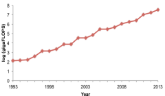
In addition, the past twenty years have also brought dramatic improvements in hardware. Figure 1 shows the exponentially increasing speed of supercomputers over the past twenty years, measured in billion floating point operations per second [1]. The hardware speedup from 1993 to 2013 is approximately . When both hardware and software improvements are considered, the overall speedup is approximately 200 billion! Note that the speedup factors cited here refer to mixed integer linear optimization problems, not MIQO problems. The speedup factors for MIQO problems are similar. MIO solvers provide both feasible solutions as well as lower bounds to the optimal value. As the MIO solver progresses towards the optimal solution, the lower bounds improve and provide an increasingly better guarantee of suboptimality, which is especially useful if the MIO solver is stopped before reaching the global optimum. In contrast, heuristic methods do not provide such a certificate of suboptimality.
The belief that MIO approaches to problems in statistics are not practically relevant was formed in the 1970s and 1980s and it was at the time justified. Given the astonishing speedup of MIO solvers and computer hardware in the last twenty-five years, the mindset of MIO as theoretically elegant but practically irrelevant is no longer justified. In this paper, we provide empirical evidence of this fact in the context of the best subset selection problem.
2.2 MIO Formulations for the Best Subset Selection Problem
We first present a simple reformulation to Problem (1) as a MIO (in fact a MIQO) problem:
| (5) |
where is a binary variable and is a constant such that if is a minimizer of Problem (5), then . If , then and if , then . Thus, is an indicator of the number of non-zeros in .
Provided that is chosen to be sufficently large with , a solution to Problem (5) will be a solution to Problem (1). Of course, is not known a priori, and a small value of may lead to a solution different from (1). The choice of affects the strength of the formulation and is critical for obtaining good lower bounds in practice. In Section 2.3 we describe how to find appropriate values for . Note that there are other MIO formulations, presented herein (See Problem (8)) that do not rely on a-priori specifications of . However, we will stick to formulation (5) for the time being, since it provides some interesting connections to the Lasso.
Formulation (5) leads to interesting insights, especially via the structure of the convex hull of its constraints, as illustrated next:
Thus, the minimum of Problem (5) is lower-bounded by the optimum objective value of both the following convex optimization problems:
| (6) | ||||||
| (7) |
where (7) is the familiar Lasso in constrained form. This is a weaker relaxation than formulation (6), which in addition to the constraint on , has box-constraints controlling the values of the ’s. It is easy to see that the following ordering exists: with the inequalities being strict in most instances.
In terms of approximating the optimal solution to Problem (5), the MIO solver begins by first solving a continuous relaxation of Problem (5). The Lasso formulation (7) is weaker than this root node relaxation. Additionally, MIO is typically able to significantly improve the quality of the root node solution as the MIO solver progresses toward the optimal solution.
To motivate the reader we provide an example of the evolution (see Figure 2) of the MIO formulation (8) for the Diabetes dataset [23], with (for further details on the dataset see Section 5).
Since formulation (5) is sensitive to the choice of , we consider an alternative MIO formulation based on Specially Ordered Sets [4] as described next.
Formulations via Specially Ordered Sets
Any feasible solution to formulation (5) will have for every . This constraint can be modeled via integer optimization using Specially Ordered Sets of Type 1 [4] (SOS-1). In an SOS-1 constraint, at most one variable in the set can take a nonzero value, that is
for every This leads to the following formulation of (1):
| (8) |
We note that Problem (8) can in principle be used to obtain global solutions to Problem (1) — Problem (8) unlike Problem (5) does not require any specification of the parameter .
 |
 |
 |
 |
| Time (secs) | Time (secs) |
We now proceed to present a more structured representation of Problem (8). Note that objective in this problem is a convex quadratic function in the continuous variable , which can be formulated explicitly as:
| (9) |
We also provide problem-dependent constants and . provides an upper bound on the absolute value of the regression coefficients and provides an upper bound on the -norm of . Adding these bounds typically leads to improved performance of the MIO, especially in delivering lower bound certificates. In Section 2.3, we describe several approaches to compute these parameters from the data.
We also consider another formulation for (9):
| (10) |
where the optimization variables are , and are problem specific parameters. Note that the objective function in formulation (10) involves a quadratic form in variables and a linear function in variables. Problem (10) is equivalent to the following variant of the best subset problem:
| (11) |
Formulations (9) and (10) differ in the size of the quadratic forms that are involved. The current state-of-the-art MIO solvers are better-equipped to handle mixed integer linear optimization problems than MIQO problems. Formulation (9) has fewer variables but a quadratic form in variables—we find this formulation more useful in the regime, with in the s. Formulation (10) on the other hand has more variables, but involves a quadratic form in variables—this formulation is more useful for high-dimensional problems , with in the s and in the s.
As we said earlier, the bounds on and are not required, but if these constraints are provided, they improve the strength of the MIO formulation. In other words, formulations with tightly specified bounds provide better lower bounds to the global optimization problem in a specified amount of time, when compared to a MIO formulation with loose bound specifications. We next show how these bounds can be computed from given data.
2.3 Specification of Parameters
Coherence and Restricted Eigenvalues of a Model Matrix
Given a model matrix , [51] introduced the cumulative coherence function
where, , represent the columns of , i.e., features.
For , we obtain the notion of coherence introduced in [22, 21] as a measure of the maximal pairwise correlation in absolute value of the columns of :
[16, 14] (see also [11] and references therein) introduced the notion that a matrix satisfies a restricted eigenvalue condition if
| (12) |
where denotes the smallest eigenvalue of the matrix . An inequality linking and is as follows.
The computations of and for general are difficult, while is simple to compute. Proposition 1 provides bounds for and in terms of the coherence .
Operator Norms of Submatrices
The operator norm of matrix is
We will use extensively here the operator norm. We assume that each column vector of has unit -norm. The results derived in the next proposition borrow and enhance techniques developed by [51] in the context of analyzing the — equivalence in compressed sensing.
Proposition 2.
For any with we have :
-
(a)
-
(b)
If the matrix is invertible and , then
Proof.
See Section A.3. ∎
We note that Part (b) also appears in [51] for the operator norm .
Given a set with we let denote the least squares regression coefficients obtained by regressing on , i.e., . If we append with zeros in the remaining coordinates we obtain as follows: Note that depends on but we will suppress the dependence on for notational convenience.
2.3.1 Specification of Parameters in terms of Coherence and Restricted Strong Convexity
Recall that , represent the columns of ; and we will use to denote the rows of . As discussed above . We order the correlations :
| (13) |
We finally denote by the sum of the top absolute values of the entries of .
Theorem 2.1.
For any such that any optimal solution to (1) satisfies:
| (14) | |||||
| (15) | |||||
| (16) | |||||
| (17) |
Proof.
For proof see Section A.4. ∎
We note that in the above theorem, the upper bound in Part (a) becomes infinite as soon as . In such a case, we can use purely data-driven bounds by using convex optimization techniques, as described in Section 2.3.2.
The interesting message conveyed by Theorem 2.1 is that the upper bounds on , and , corresponding to the Problem (11) can all be obtained in terms of and , quantities of fundamental interest appearing in the analysis of regularization methods and understanding how close they are to solutions [51, 22, 21, 16, 14]. On a different note, Theorem 2.1 arises from a purely computational motivation and quite curiously, involves the same quantities: cumulative coherence and restricted eigenvalues.
Note that the quantities are difficult to compute exactly, but they can be approximated by Proposition 1 which provides bounds commonly used in the compressed sensing literature. Of course, approximations to these quantities can also be obtained by using subsampling schemes.
2.3.2 Specification of Parameters via Convex Quadratic Optimization
We provide an alternative purely data-driven way to compute the upper bounds to the parameters by solving several simple convex quadratic optimization problems.
Bounds on ’s
For the case , upper and lower bounds on can be obtained by solving the following pair of convex optimization problems:
| (18) |
for . Above, UB is an upper bound to the minimum of the -subset least squares problem (1). is an upper bound to , since the cardinality constraint does not appear in the optimization problem. Similarly, is a lower bound to . The quantity serves as an upper bound to . A reasonable choice for UB is obtained by using the discrete first order methods (Algorithms 1 and 2 as described in Section 3) in combination with the MIO formulation (8) (for a predefined amount of time). Having obtained as described above, we can obtain an upper bound to and as follows: and where, .
Similarly, bounds corresponding to Parts (c) and (d) in Theorem 2.1 can be obtained by using the upper bounds on as described above.
Note that the quantities and are finite when the level sets of the least squares loss function are finite. In particular, the bounds are loose when . In the following we describe methods to obtain non-trivial bounds on , for that apply for arbitrary .
Bounds on ’s
We now provide a generic method to obtain upper and lower bounds on the quantities :
| (19) |
for . Note that the bounds obtained from (19) are non-trivial bounds for both the under-determined and overdetermined cases. The bounds obtained from (19) are upper and lower bounds since we drop the cardinality constraint on . The bounds are finite since for every the quantity remains bounded in the feasible set for Problems (19).
2.3.3 Parameter Specifications from Advanced Warm-Starts
The methods described above in Sections 2.3.1 and 2.3.2 lead to provable bounds on the parameters: with these bounds Problem (11) is provides an optimal solution to Problem (1), and vice-versa. We now describe some other alternatives that lead to excellent parameter specifications in practice.
The discrete first order methods described in the following section 3 provide good upper bounds to Problem (1). These solutions when supplied as a warm-start to the MIO formulation (8) are often improved by MIO, thereby leading to high quality solutions to Problem (1) within several minutes. If denotes an estimate obtained from this hybrid approach, then with a multiplier greater than one (e.g., ) provides a good estimate for the parameter . A reasonable upper bound to is . Bounds on the other quantities: can be derived by using expressions appearing in Theorem 2.1, with aforementioned bounds on and .
2.3.4 Some Generalizations and Variants
Some variations and improvements of the procedures described above are presented in Section A.2 (appendix).
3 Discrete First Order Algorithms
In this section, we develop a discrete extension of first order methods in convex optimization [45, 44] to obtain near optimal solutions for Problem (1) and its variant for the least absolute deviation (LAD) loss function. Our approach applies to the problem of minimizing any smooth convex function subject to cardinality constraints.
We will use these discrete first order methods to obtain solutions to warm start the MIO formulation. In Section 5, we will demonstrate how these methods greatly enhance the performance of the MIO.
3.1 Finding stationary solutions for minimizing smooth convex functions with cardinality constraints
Related work and contributions
In the signal processing literature [8, 9] proposed iterative hard-thresholding algorithms, in the context of -regularized least squares problems, i.e., Problem (4). The authors establish convergence properties of the algorithm under the assumption that satisfies coherence [8] or Restricted Isometry Property [9]. The method we propose here applies to a larger class of cardinality constrained optimization problems of the form (20), in particular, in the context of Problem (1) our algorithm and its convergence analysis do not require any form of restricted isometry property on the model matrix .
Our proposed algorithm borrows ideas from projected gradient descent methods in first order convex optimization problems [45] and generalizes it to the discrete optimization Problem (20). We also derive new global convergence results for our proposed algorithms as presented in Theorem 3.1. Our proposal, with some novel modifications also applies to the non-smooth least absolute deviation loss with cardinality constraints as discussed in Section 3.3.
Consider the following optimization problem:
| (20) |
where is convex and has Lipschitz continuous gradient:
| (21) |
The first ingredient of our approach is the observation that when for a given , Problem (20) admits a closed form solution.
Proposition 3.
If is an optimal solution to the following problem:
| (22) |
then it can be computed as follows: retains the largest (in absolute value) elements of and sets the rest to zero, i.e., if denote the ordered values of the absolute values of the vector , then:
| (23) |
where, is the th coordinate of . We will denote the set of solutions to Problem (22) by the notation .
Proof.
We provide a proof of this in Section B.2, for the sake of completeness. ∎
Note that, we use the notation “argmin” (Problem (22) and in other places that follow) to denote the set of minimizers of the optimization Problem.
The operator (23) is also known as the hard-thresholding operator [20]—a notion that arises in the context of the following related optimization problem:
| (24) |
where admits a simple closed form expression given by if and otherwise, for .
Remark 1.
There is an important difference between the minimizers of Problems (22) and (24). For Problem (24), the smallest (in absolute value) non-zero element in is greater than in absolute value. On the other hand, in Problem (22) there is no lower bound to the minimum (in absolute value) non-zero element of a minimizer. This needs to be taken care of while analyzing the convergence properties of Algorithm 1 (Section 3.2).
Given a current solution , the second ingredient of our approach is to upper bound the function around . To do so, we use ideas from projected gradient descent methods in first order convex optimization problems [45, 44].
Proposition 4.
Algorithm 1
Input: , , .
Output: A first order stationary solution .
Algorithm:
-
1.
Initialize with such that .
-
2.
For , apply (26) with to obtain as:
(27) -
3.
Repeat Step 2, until .
-
4.
Let denote the current estimate and let . Solve the continuous optimization problem:
(28) and let be a minimizer.
The convergence properties of Algorithm 1 are presented in Section 3.2. We also present Algorithm 2, a variant of Algorithm 1 with better empirical performance. Algorithm 2 modifies Step 2 of Algorithm 1 by using a line search. It obtains and where .
Note that the iterate in Algorithm 2 need not be -sparse (i.e., need not satisfy: ), however, is -sparse (). Moreover, the sequence may not lead to a decreasing set of objective values, but it satisfies:
3.2 Convergence Analysis of Algorithm 1
In this section, we study convergence properties for Algorithm 1. Before we embark on the analysis, we need to define the notion of first order optimality for Problem (20).
Definition 1.
Given an , the vector is said to be a first order stationary point of Problem (20) if and it satisfies the following fixed point equation:
| (29) |
Let us give some intuition associated with the above definition.
Consider as in Definition 1. Since it follows that there is a set such that for all and the size of (complement of ) is . Since it follows that for all , we have: where, is the th coordinate of . It thus follows that: for all . Since is convex in , this means that solves the following convex optimization problem:
| (30) |
Note however, that the converse of the above statement is not true. That is, if is an arbitrary subset with then a solution to the restricted convex problem (30) with need not correspond to a first order stationary point.
Note that any global minimizer to Problem (20) is also a first order stationary point, as defined above (see Proposition 7).
We present the following proposition (for its proof see Section B.6), which sheds light on a first order stationary point for which .
Proposition 5.
Suppose satisfies the first order stationary condition (29) and . Then .
We next define the notion of an -approximate first order stationary point of Problem (20):
Definition 2.
Given an and we say that satisfies an -approximate first order optimality condition of Problem (20) if and for some , we have .
Before we dive into the convergence properties of Algorithm 1, we need to introduce some notation. Let and with , if , and , if , , i.e., represents the sparsity pattern of the support of .
Suppose, we order the coordinates of by their absolute values: . Note that by definition (27), for all and . We denote to be the th largest (in absolute value) entry in for all . Clearly if then and if then . Let and .
Proposition 6.
Consider and as defined in (20) and (21). Let be the sequence generated by Algorithm 1. Then we have :
-
(a)
For any , the sequence satisfies
(31) is decreasing and converges.
-
(b)
If , then as .
-
(c)
If and then the sequence converges after finitely many iterations, i.e., there exists an iteration index such that for all . Furthermore, the sequence is bounded and converges to a first order stationary point.
-
(d)
If and then .
-
(e)
Let , and suppose that the sequence has a limit point. Then .
Proof.
See Section B.1. ∎
Remark 2.
Note that the existence of a limit point in Proposition 6, Part (e) is guaranteed under fairly weak conditions. One such condition is that for any finite value . In words this means that the -sparse level sets of the function is bounded.
In the special case where is the least squares loss function, the above condition is equivalent to every -submatrix () of comprising of columns being full rank. In particular, this holds with probability one when the entries of are drawn from a continuous distribution and .
Remark 3.
Parts (d) and (e) of Proposition 6 are probably not statistically interesting cases, since they correspond to un-regularized solutions of the problem . However, we include them since they shed light on the properties of Algorithm 1.
The conditions assumed in Part (c) imply that the support of stabilizes and Algorithm 1 behaves like vanilla gradient descent thereafter. The support of need not stabilize for Parts (d), (e) and thus Algorithm 1 may not behave like vanilla gradient descent after finitely many iterations. However, the objective values (under minor regularity assumptions) converge to .
We present the following Proposition (for proof see Section B.3) about a uniqueness property of the fixed point equation (1).
Proposition 7.
Suppose and let satisfy a first order stationary point as in Definition 1. Then the set has exactly one element: .
The following proposition (for a proof see Section B.4) shows that a global minimizer of the Problem (20) is also a first order stationary point.
Proposition 8.
Suppose and let be a global minimizer of Problem (20). Then is a first order stationary point.
Proposition 6 establishes that Algorithm 1 either converges to a first order stationarity point (part (c)) or it converges111under minor technical assumptions to a global optimal solution (Parts (d), (e)), but does not quantify the rate of convergence. We next characterize the rate of convergence of the algorithm to an -approximate first order stationary point.
Theorem 3.1.
Let and denote a first order stationary point of Algorithm 1. After iterations Algorithm 1 satisfies
| (32) |
where as .
Proof.
See Section B.5. ∎
Theorem 3.1 implies that for any there exists such that for some , we have: Note that the convergence rates derived above apply for a large class of problems (20), where, the function is convex with Lipschitz continuous gradient (21). Tighter rates may be obtained under additional structural assumptions on . For example, the adaptation of Algorithm 1 for Problem (4) was analyzed in [8, 9] with satisfying coherence [8] or Restricted Isometry Property (RIP) [9]. In these cases, the algorithm can be shown to have a linear convergence rate [8, 9], where the rate depends upon the RIP constants.
Note that by Proposition 6 the support of stabilizes after finitely many iterations, after which Algorithm 1 behaves like gradient descent on the stabilized support. If restricted to this support is strongly convex, then Algorithm 1 will enjoy a linear rate of convergence [45], as soon as the support stabilizes. This behavior is adaptive, i.e., Algorithm 1 does not need to be modified after the support stabilizes.
The next section describes practical post-processing schemes via which first order stationary points of Algorithm 1 can be obtained by solving a low dimensional convex optimization problem, as soon as the support is found to stabilize, numerically. In our numerical experiments, we this version of Algorithm 1 (with multiple starting points) took at most a few minutes for and a few seconds for smaller values of .
Polishing coefficients on the active set
Algorithm 1 detects the active set after a few iterations. Once the active set stabilizes, the algorithm may take a number of iterations to estimate the values of the regression coefficients on the active set to a high accuracy level.
In this context, we found the following simple polishing of coefficients to be useful. When the algorithm has converged to a tolerance of (), we fix the current active set, , and solve the following lower-dimensional convex optimization problem:
| (33) |
In the context of the least squares and the least absolute deviation problems, Problem (33) reduces to to a smaller dimensional least squares and a linear optimization problem respectively, which can be solved very efficiently up to a very high level of accuracy.
3.3 Application to Least Squares
For the support constrained problem with squared error loss, we have and . The general algorithmic framework developed above applies in a straightforward fashion for this special case. Note that for this case .
The polishing of the regression coefficients in the active set can be performed via a least squares problem on , where denotes the support of the regression coefficients.
3.4 Application to Least Absolute Deviation
We will now show how the method proposed in the previous section applies to the least absolute deviation problem with support constraints in :
| (34) |
Since is non-smooth, our framework does not apply directly. We smooth the non-differentiable so that we can apply Algorithms 1 and 2. Observing that we make use of the smoothing technique of [43] to obtain ; which is a smooth approximation of , with for which Algorithms 1 and 2 apply.
In order to obtain a good approximation to Problem (34), we found the following strategy to be useful in practice:
-
1.
Fix , initialize with and repeat the following steps [2]—[3] till convergence:
-
2.
Apply Algorithm 1 (or Algorithm 2) to the smooth function . Let be the limiting solution.
-
3.
Decrease for some pre-defined constant (say), and go back to step [1] with . Exit if for some pre-defined tolerance.
4 A Brief Tour of the Statistical Properties of Problem (1)
As already alluded to in the introduction, there is a substantial body of impressive work characterizing the theoretical properties of best subset solutions in terms of various metrics: predictive performance, estimation of regression coefficients, and variable selection properties. For the sake of completeness, we present a brief review of some of the properties of solutions to Problem (1) in Section C.
5 Computational Experiments for Subset Selection with Least Squares Loss
In this section, we present a variety of computational experiments to assess the algorithmic and statistical performances of our approach. We consider both the classical overdetermined case with (Section 5.2) and the high dimensional case (Section 5.3) for the least squares loss function with support constraints.
5.1 Description of Experimental Data
We demonstrate the performance of our proposal via a series of experiments on both synthetic and real data.
Synthetic Datasets.
We consider a collection of problems where are independent realizations from a -dimensional multivariate normal distribution with mean zero and covariance matrix . The columns of the matrix were subsequently standardized to have unit norm. For a fixed we generated the response as follows: , where . We denote the number of nonzeros in by . The choice of determines the Signal-to-Noise Ratio (SNR) of the problem, which is defined as:
We considered the following four different examples:
Example 1: We took for . We consider different values of and for equi-spaced values. In the case where exactly equi-spaced values are not possible we rounded the indices to the nearest large integer value. of in the range .
Example 2: We took , and .
Example 3: We took , and and — i.e., a vector with ten nonzero entries, with the nonzero values being equally spaced in the interval .
Example 4: We took , and , i.e., a vector with six nonzero entries, equally spaced in the interval .
Real Datasets
We considered the Diabetes dataset analyzed in [23]. We used the dataset with all the second order interactions included in the model, which resulted in 64 predictors. We reduced the sample size to by taking a random sample and standardized the response and the columns of the model matrix to have zero means and unit -norm.
In addition to the above, we also considered a real microarray dataset: the Leukemia data [18]. We downloaded the processed dataset from http://stat.ethz.ch/~dettling/bagboost.html, which had binary responses and more than 3000 predictors. We standardized the response and columns of features to have zero means and unit -norm. We reduced the set of features to 1000 by retaining the features maximally correlated (in absolute value) to the response. We call the resulting feature matrix with . We then generated a semi-synthetic dataset with continuous response as , where the first five coefficients of were taken as one and the rest as zero. The noise was distributed as , with chosen to get a SNR=7.
Computer Specifications and Software
Computations were carried out in a linux 64 bit server—Intel(R) Xeon(R) eight-core processor @ 1.80GHz, 16 GB of RAM for the overdetermined case and in a Dell Precision T7600 computer with an Intel Xeon E52687 sixteen-core processor @ 3.1GHz, 128GB of Ram for the high-dimensional case. The discrete first order methods were implemented in Matlab 2012b. We used Gurobi [33] version 5.5 and the Matlab interface to Gurobi for all of our experiments, apart from the computations for synthetic data for , which were done in Gurobi via its Python 2.7 interface.
5.2 The Overdetermined Regime:
Using the Diabetes dataset and synthetic datasets, we demonstrate the combined effect of using the discrete first order methods with the MIO approach. Together, these methods show improvements in obtaining good upper bounds and in closing the MIO gap to certify global optimality. Using synthetic datasets where we know the true linear regression model, we perform side-by-side comparisons of this method with several other state-of-the-art algorithms designed to estimate sparse linear models.
5.2.1 Obtaining Good Upper Bounds
We conducted experiments to evaluate the performance of our methods in terms of obtaining high quality solutions for Problem (1).
We considered the following three algorithms:
-
(a)
Algorithm 2 with fifty random initializations222we took fifty random starting values around of the form , where . We found empirically that Algorithm 2 provided better upper bounds than Algorithm 1.. We took the solution corresponding to the best objective value.
-
(b)
MIO with cold start, i.e., formulation (9) with a time limit of seconds.
-
(c)
MIO with warm start. This was the MIO formulation initialized with the discrete first order optimization solution obtained from (a). This was run for a total of 500 seconds.
To compare the different algorithms in terms of the quality of upper bounds, we run for every instance all the algorithms and obtain the best solution among them, say, . If denotes the value of the best subset objective function for method “alg”, then we define the relative accuracy of the solution obtained by “alg” as:
| (35) |
where as described above.
We did experiments for the Diabetes dataset for different values of (see Table 1). For each of the algorithms we report the amount of time taken by the algorithm to reach the best objective value during the time of seconds.
| Discrete First Order | MIO Cold Start | MIO Warm Start | ||||
| Accuracy | Time | Accuracy | Time | Accuracy | Time | |
| 9 | 0.1306 | 1 | 0.0036 | 500 | 0 | 346 |
| 20 | 0.1541 | 1 | 0.0042 | 500 | 0 | 77 |
| 49 | 0.1915 | 1 | 0.0015 | 500 | 0 | 87 |
| 57 | 0.1933 | 1 | 0 | 500 | 0 | 2 |
Using the discrete first order methods in combination with the MIO algorithm resulted in finding the best possible relative accuracy in a matter of a few minutes.
5.2.2 Improving MIO Performance via Warm Starts
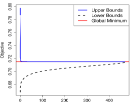
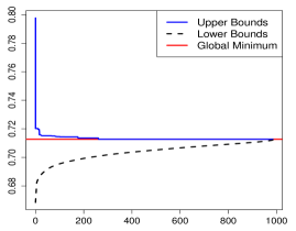
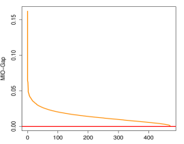
We performed a series of experiments on the Diabetes dataset to obtain a globally optimal solution to Problem (1) via our approach and to understand the implications of using advanced warm starts to the MIO formulation in terms of certifying optimality. For each choice of we ran Algorithm 2 with fifty random initializations. They took less than a few seconds to run. We used the best solution as an advanced warm start to the MIO formulation (9). For each of these examples, we also ran the MIO formulation without any warm start information and also without the parameter specifications in Section 2.3 (we refer to this as “cold start”). Figure 3 summarizes the results. The figure shows that in the presence of warm starts and problem specific side information, the MIO closes the optimality gap significantly faster.
| k=9 | k=20 | k=31 | k=42 |
 |
 |
 |
 |
| Time (secs) | Time (secs) | Time (secs) | Time (secs) |
5.2.3 Statistical Performance
We considered datasets as described in Example 1, Section 5.1—we took different values of with , with .
Competing Methods and Performance Measures
For every example, we considered the following learning procedures for comparison purposes: (a) the MIO approach equipped warm starts from Algorithm 2 (annotated as “MIO” in the figure), (b) the Lasso, (c) Sparsenet and (d) stepwise regression (annotated as “Step” in the figure).
We used R to compute Lasso, Sparsenet and stepwise regression using the glmnet 1.7.3, Sparsenet and Stats 3.0.2 packages respectively, which were all downloaded from CRAN at http://cran.us.r-project.org/.
In addition to the above, we have also performed comparisons with a debiased version of the Lasso: i.e., performing unrestricted least squares on the Lasso support to mitigate the bias imparted by Lasso shrinkage.
We note that Sparsenet [38] considers a penalized likelihood formulation of the form (3), where the penalty is given by the generalized MCP penalty family (indexed by ) for a family of values of and . The family of penalties used by Sparsenet is thus given by: for described as above. As with fixed, we get the penalty . The family above includes as a special case (), the hard thresholding penalty, a penalty recommended in the paper [60] for its useful statistical properties.
For each procedure, we obtained the “optimal” tuning parameter by selecting the model that achieved the best predictive performance on a held out validation set. Once the model was selected, we obtained the prediction error as:
| (36) |
We report “prediction error” and number of non-zeros in the optimal model in our results. The results were averaged over ten random instances, for different realizations of . For every run: the training and validation data had a fixed but random noise .
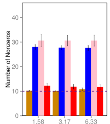
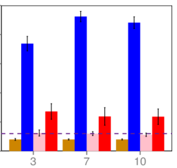
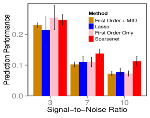
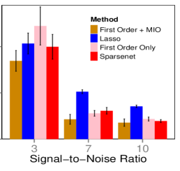
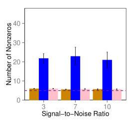
Figure 4 presents results for data generated as per Example 1 with = 500 and = 100. We see that the MIO procedure performs very well across all the examples. Among the methods, MIO performs the best, followed by Sparsenet, Lasso with Step(wise) exhibiting the worst performance. In terms of prediction error, the MIO performs the best, only to be marginally outperformed by Sparsenet in a few instances. This further illustrates the importance of using non-convex methods in sparse learning. Note that the MIO approach, unlike Sparsenet certifies global optimality in terms of solving Problem 1. However, based on the plots in the upper panel, Sparsenet selects a few redundant variables unlike MIO. Lasso delivers quite dense models and pays the price in predictive performance too, by selecting wrong variables. As the value of SNR increases, the predictive power of the methods improve, as expected. The differences in predictive errors between the methods diminish with increasing SNR values. With increasing values of (from left panel to right panel in the figure), the number of non-zeros selected by the Lasso in the optimal model increases.
We also performed experiments with the debiased version of the Lasso. The unrestricted least squares solution on the optimal model selected by Lasso (as shown in Figure 4) had worse predictive performance than the Lasso, with the same sparsity pattern. This is probably due to overfitting since the model selected by the Lasso is quite dense compared to . We also tried some variants of debiased Lasso which led to models with better performances than the Lasso but the results were inferior compared to MIO — we provide a detailed description in Section D.2.
 |
 |
 |
 |
 |
 |
We also performed experiments with for data generated as per Example 1. We solved the problems to provable optimality and found that the MIO performed very well when compared to other competing methods. We do not report the experiments for brevity.
5.2.4 MIO model training
We trained a sequence of best subset models (indexed by ) by applying the MIO approach with warm starts. Instead of running the MIO solvers from scratch for different values of , we used callbacks, a feature of integer optimization solvers. Callbacks allow the user to solve an initial model, and then add additional constraints to the model one at a time. These “cuts” reduce the size of the feasible region without having to rebuild the entire optimization model. Thus, in our case, we can save time by building the initial optimization model for . Once the solution for is obtained, a cut can be added to the model: for and the model can be re-solved from this point. We apply this procedure until we arrive at a model with .
For each value of tested, the MIO best subset algorithm was set to stop the first time either an optimality gap of 1% was reached or a time limit of 15 minutes was reached. Additionally, we only tested values of from 5 through 25, and used Algorithm 2 to warm start the MIO algorithm. We observed that it was possible to obtain speedups of a factor of 2-4 by carefully tuning the optimization solver for a particular problem, but chose to maintain generality by solving with default parameters. Thus, we do not report times with the intention of accurately benchmarking the best possible time but rather to show that it is computationally tractable to solve problems to optimality using modern MIO solvers.
5.3 The High-Dimensional Regime:
In this section, we investigate (a) the evolution of upper bounds in the high-dimensional regime, (b) the effect of a bounding box formulation on the speed of closing the optimality gap and (c) the statistical performance of the MIO approach in comparison to other state-of-the art methods.
5.3.1 Obtaining Good Upper Bounds
We performed tests similar to those in Section 5.2.1 for the regime. We tested a synthetic dataset corresponding to Example 2 with for varying SNR values (see Table 2) over a time of 500s. As before, using the discrete first order methods in combination with the MIO algorithm resulted in finding the best possible upper bounds in the shortest possible times.
| Discrete First Order | MIO Cold Start | MIO Warm Start | |||||
| Accuracy | Time | Accuracy | Time | Accuracy | Time | ||
| 5 | 0.1647 | 37.2 | 1.0510 | 500 | 0 | 72.2 | |
| 6 | 0.6152 | 41.1 | 0.2769 | 500 | 0 | 77.1 | |
| 7 | 0.7843 | 40.7 | 0.8715 | 500 | 0 | 160.7 | |
|
SNR = 3 |
8 | 0.5515 | 38.8 | 2.1797 | 500 | 0 | 295.8 |
| 9 | 0.7131 | 45.0 | 0.4204 | 500 | 0 | 96.0 | |
| 5 | 0.5072 | 45.6 | 0.7737 | 500 | 0 | 65.6 | |
| 6 | 1.3221 | 40.3 | 0.5121 | 500 | 0 | 82.3 | |
| 7 | 0.9745 | 40.9 | 0.7578 | 500 | 0 | 210.9 | |
|
SNR = 7 |
8 | 0.8293 | 40.5 | 1.8972 | 500 | 0 | 262.5 |
| 9 | 1.1879 | 44.2 | 0.4515 | 500 | 0 | 254.2 | |
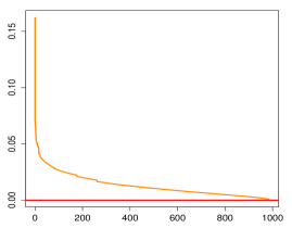
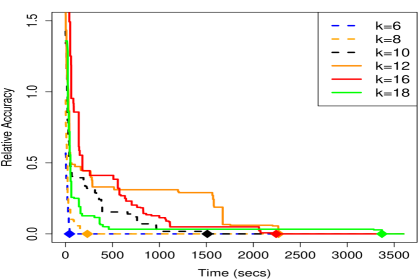
We also did experiments on the Leukemia dataset. In Figure 5 we demonstrate the evolution of the objective value of the best subset problem for different values of . For each value of , we warm-started the MIO with the solution obtained by Algorithm 2 and allowed the MIO solver to run for 4000 seconds. The best objective value obtained at the end of 4000 seconds is denoted by . We plot the Relative Accuracy, i.e., , where is the objective value obtained after seconds. The figure shows that the solution obtained by Algorithm 2 is improved by the MIO on various instances and the time taken to improve the upper bounds depends upon . In general, for smaller values of the upper bounds obtained by the MIO algorithm stabilize earlier, i.e., the MIO finds improved solutions faster than larger values of .
5.3.2 Bounding Box Formulation
With the aid of advanced warm starts as provided by Algorithm 2, the MIO obtains a very high quality solution very quickly—in most of the examples the solution thus obtained turns out to be the global minimum. However, in the typical “high-dimensional” regime, with , we observe that the certificate of global optimality comes later as the lower bounds of the problem “evolve” slowly. This is observed even in the presence of warm starts and using the implied bounds as developed in Section 2.2 and is aggravated for the cold-started MIO formulation (10).
To address this, we consider the MIO formulation (37) obtained by adding bounding boxes around a local solution. These restrictions guide the MIO in restricting its search space and enable the MIO to certify global optimality inside that bounding box. We consider the following additional bounding box constraints to the MIO formulation (10):
where, is a candidate sparse solution. The radii of the two -balls above, namely, and are user-defined parameters and control the size of the feasible set.
Using the notation we have the following MIO formulation (equipped with the additional bounding boxes):
| (37) |
For large values of (respectively, ) the constraints on (respectively, ) become ineffective and one gets back formulation (10). To see the impact of these additional cutting planes in the MIO formulation, we consider a few examples as illustrated in Figures 6,7,12.
Interpretation of the bounding boxes
A local bounding box in the variable directs the MIO solver to seek for candidate solutions that deliver models with predictive accuracy “similar” (controlled by the radius of the ball) to a reference predictive model, given by . In our experiments, we typically chose as the solution delivered by running MIO (warm-started with a first order solution) for a few hundred to a few thousand seconds. More generally, may be selected by any other sparse learning method. In our experiments, we found that the run-time behavior of the MIO depends upon how correlated the columns of are — more correlation leading to longer run-times.
Similarly, a bounding box around directs the MIO to look for solutions in the neighborhood of a reference point . In our experiments, we chose the reference as the solution obtained by MIO (warm-started with a first order solution) and allowing it to run for a few hundred to a few thousand seconds. We observed that the MIO solver in presence of bounding boxes in the -space certified optimality and in the process finding better solutions; much faster than the -bounding box method.
Note that the -bounding box constraint leads to and the -box leads to constraints. Thus, when the additional constraints add a fewer number of extra variables when compared to the constraints.
Experiments
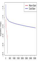
In the first set of experiments, we consider the Leukemia dataset with . We took two different values of and for each case we ran Algorithm 2 with several random restarts. The best solution thus obtained was used to warm start the MIO formulation (10), which we ran for an additional 3600 seconds. The solution thus obtained is denoted by . We then consider formulation (37) with and different values of (as annotated in Figure 6) — the results are displayed in Figure 6.
| Leukemia dataset: Effect of a Bounding Box for MIO formulation (37) | |
 |
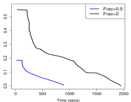 |
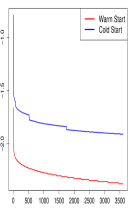
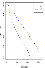
We consider another set of experiments to demonstrate the performance of the MIO in certifying global optimality for different synthetic datasets with varying as well as with different structures on the bounding box. In the first case, we generated data as per Example 1 with , . We consider the case with , and , where is a -sparse solution obtained from the MIO formulation (10) run with a time limit of 1000 seconds, after being warm-started with Algorithm 2. The results are displayed in Figure 7[Left Panel]. In the second case (with data same as before) we obtained in the same fashion as described before—we took a bounding box around , and left the box constraint around inactive, i.e., we set and . We performed two sets of experiments, where the data were generated based on different SNR values—the results are displayed in Figure 7 with SNR=1 [Middle Panel] and SNR = 3[Right Panel].
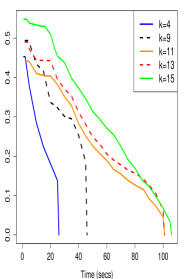
In the same vein, we have Figure 12 studying the effect of formulations (37) for synthetic datasets generated as per Example 1 with and .
| Evolution of the MIO gap for (37), effect of type of bounding box (). | ||
|---|---|---|
 |
 |
 |
5.3.3 Statistical Performance
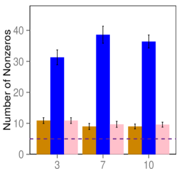
To understand the statistical behavior of MIO when compared to other approaches for learning sparse models, we considered synthetic datasets for values of ranging from and values of ranging from . The following methods were used for comparison purposes (a) Algorithm 2. Here we used fifty different random initializations around , of the form and took the solution corresponding to the best objective value; (b) The MIO approach with warm starts from part (a); (c) The Lasso solution and (d) The Sparsenet solution.
For methods (a), (b) we considered ten equi-spaced values of in the range (including the optimal value of ). For each of the methods, the best model was selected in the same fashion as described in Section 5.2.3 using separate validation sets.
In addition, for some examples, we also study the performance of the debiased version of the Lasso, as described in Section 5.2.3.
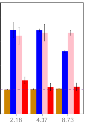
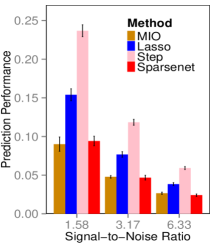
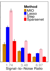
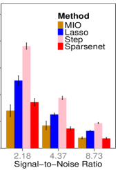
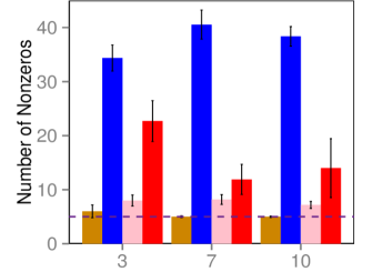
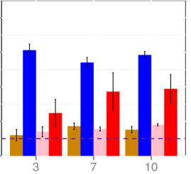
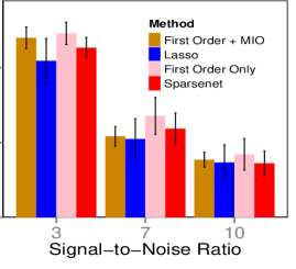
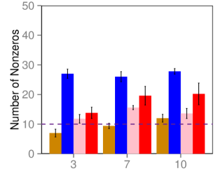
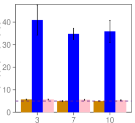
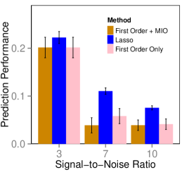
In Figure 8 and Figure 9 we present selected representative results from four different examples described in Section 5.1.
 |
 |
 |
 |
 |
 |
 |
 |
In Figure 8 the left panel shows the performance of different methods for Example 1 with . In this example, there are five non-zero coefficients: the features corresponding to the non-zero coefficients are weakly correlated and a feature having a non-zero coefficient is highly correlated with a feature having a zero coefficient. In this situation, the Lasso selects a very dense model since it fails to distinguish between a zero and a non-zero coefficient when the variables are correlated—it brings both the coefficients in the model (with shrinkage). MIO (with warm-start) performs the best—both in terms of predictive accuracy and in selecting a sparse set of coefficients. MIO obtains the sparsest model among the four methods and seems to find better solutions in terms of statistical properties than the models obtained by the first order methods alone. Interestingly, the “optimal model” selected by the first order methods is more dense than that selected by the MIO. The number of non-zero coefficients selected by MIO remains fairly stable across different SNR values, unlike the other three methods. For this example, we also experimented with the different versions of debiased Lasso. In summary: the best debiased Lasso models had performance marginally better than Lasso but quite inferior to MIO. See the results in Appendix, Section D.2 for further details.
In Figure 8 the right panel shows Example 2, with and all non-zero coefficients equal one. In this example, all the methods perform similarly in terms of predictive accuracy. This is because all non-zero coefficients in have the same value. In fact for the smallest value of SNR, the Lasso achieves the best predictive model. In all the cases however, the MIO achieves the sparsest model with favorable predictive accuracy.
In Figure 9, for both the examples, the model matrix is an iid Gaussian ensemble. The underlying regression coefficient however, is structurally different than Example 2 (as in Figure 8, right-panel). The structure in is responsible for different statistical behaviors of the four methods across Figures 8 (right-panel) and Figure 9 (both panels). The alternating signs and varying amplitudes of are responsible for the poor behavior of Lasso. The MIO (with warm-starts) seems to be the best among all the methods. For Example 3 (Figure 9, left panel) the predictive performances of Lasso and MIO are comparable—the MIO however delivers much sparser models than the Lasso.
The key conclusions are as follows:
-
1.
The MIO best subset algorithm has a significant edge in detecting the correct sparsity structure for all examples compared to Lasso, Sparsenet and the stand-alone discrete first order method.
-
2.
For data generated as per Example 1 with large values of , the MIO best subset algorithm gives better predictive performance compared to its competitors.
-
3.
For data generated as per Examples 2 and 3, MIO delivers similar predictive models like the Lasso, but produces much sparser models. In fact, Lasso seems to perform marginally better than MIO, as a predictive model for small values of SNR.
-
4.
For Example 4, MIO performs the best both in terms of predictive accuracy and delivering sparse models.
6 Computational Results for Subset Selection with Least Absolute Deviation Loss
In this section, we demonstrate how our method can be used for the best subset selection problem with LAD objective (34).
Since the main focus of this paper is the least squares loss function, we consider only a few representative examples for the LAD case. The LAD loss is appropriate when the error follows a heavy tailed distribution. The datasets used for the experiments parallel those described in Section 5.1, the difference being in the distribution of . We took iid from a double exponential distribution with variance . The value of was adjusted to get different values of SNR.
Datasets analysed
We consider a set-up similar to Example 1 (Section 5.1) with and . Different choices of were taken to cover both the overdetermined () and high-dimensional cases ( and ).
The other competing methods used for comparison were (a) discrete first order method (Section (3.4)) (b) MIO warm-started with the first order solutions and (c) the LAD loss with regularization:
which we denote by LAD-Lasso. The training, validation and testing were done in the same fashion as in the least squares case. For each method, we report the number of non-zeros in the optimal model and associated prediction accuracy (36).
 |
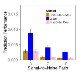 |
Figure 10 compares the MIO approach with others for LAD in the overdetermined case (). Figure 11 does the same for the high-dimensional case (). The conclusions parallel those for the least squares case. Since, in the example considered, the features corresponding to the non-zero coefficients are weakly correlated and a feature having a non-zero coefficient is highly correlated with a feature having a zero coefficient—the LAD-Lasso selects an overly dense model and misses out in terms of prediction error. Both the MIO (with warm-starts) and the discrete first order methods behave similarly—much better than regularization schemes. As expected, we observed that subset selection with least squares loss leads to inferior models for these examples, due to a heavy-tailed distribution of the errors.
The results in this section are similar to the least squares case. The MIO approach provides an edge both in terms of sparsity and predictive accuracy compared to Lasso both for the overdetermined and the high-dimensional case.

7 Conclusions
In this paper, we have revisited the classical best subset selection problem of choosing out of features in linear regression given observations using a modern optimization lens, i.e., MIO and a discrete extension of first order methods from continuous optimization. Exploiting the astonishing progress of MIO solvers in the last twenty-five years, we have shown that this approach solves problems with in the 1000s and in the 100s in minutes to provable optimality, and finds near optimal solutions for in the 100s and in the 1000s in minutes. Importantly, the solutions provided by the MIO approach significantly outperform other state of the art methods like Lasso in achieving sparse models with good predictive power. Unlike all other methods, the MIO approach always provides a guarantee on its sub-optimality even if the algorithm is terminated early. Moreover, it can accommodate side constraints on the coefficients of the linear regression and also extends to finding best subset solutions for the least absolute deviation loss function.
While continuous optimization methods have played and continue to play an important role in statistics over the years, discrete optimization methods have not. The evidence in this paper as well as in [2] suggests that MIO methods are tractable and lead to desirable properties (improved accuracy and sparsity among others) at the expense of higher, but still reasonable, computational times.
Acknowledgements
We would like to thank the Associate editor and two reviewers for their comments that helped us improve the paper. A major part of the work was performed when R.M. was at Columbia University.
References
- [1] Top500 Supercomputer Sites, Directory page for Top500 lists. Result for each list since June 1993. http://www.top500.org/statistics/sublist/. Accessed: 2013-12-04.
- Bertsimas and Mazumder [2014] D. Bertsimas and R. Mazumder. Least quantile regression via modern optimization. The Annals of Statistics, 42(6):2494–2525, 2014.
- Bertsimas and Shioda [2009] D. Bertsimas and R. Shioda. Algorithm for cardinality-constrained quadratic optimization. Computational Optimization and Applications, 43(1):1–22, 2009.
- Bertsimas and Weismantel [2005] D. Bertsimas and R. Weismantel. Optimization over integers. Dynamic Ideas Belmont, 2005.
- Bickel et al. [2009] P. Bickel, Y. Ritov, and A. Tsybakov. Simultaneous analysis of lasso and dantzig selector. The Annals of Statistics, pages 1705–1732, 2009.
- Bienstock [1996] D. Bienstock. Computational study of a family of mixed-integer quadratic programming problems. Mathematical programming, 74(2):121–140, 1996.
- Bixby [2012] R. E. Bixby. A brief history of linear and mixed-integer programming computation. Documenta Mathematica, Extra Volume: Optimization Stories, pages 107–121, 2012.
- Blumensath and Davies [2008] T. Blumensath and M. Davies. Iterative thresholding for sparse approximations. Journal of Fourier Analysis and Applications, 14(5-6):629–654, 2008.
- Blumensath and Davies [2009] T. Blumensath and M. Davies. Iterative hard thresholding for compressed sensing. Applied and Computational Harmonic Analysis, 27(3):265–274, 2009.
- Boyd and Vandenberghe [2004] S. Boyd and L. Vandenberghe. Convex Optimization. Cambridge University Press, Cambridge, 2004.
- Bühlmann and van-de-Geer [2011] P. Bühlmann and S. van-de-Geer. Statistics for high-dimensional data. Springer, 2011.
- Bunea et al. [2007] F. Bunea, A. B. Tsybakov, M. H. Wegkamp, et al. Aggregation for gaussian regression. The Annals of Statistics, 35(4):1674–1697, 2007.
- Candes et al. [2008] E. Candes, M. Wakin, and S. Boyd. Enhancing sparsity by reweighted minimization. Journal of Fourier Analysis and Applications, 14(5):877–905, 2008.
- Candes [2008] E. Candes. The restricted isometry property and its implications for compressed sensing. Comptes Rendus Mathematique, 346(9):589–592, 2008.
- Candès and Plan [2009] E. Candès and Y. Plan. Near-ideal model selection by minimization. The Annals of Statistics, 37(5A):2145–2177, 2009.
- Candes and Tao [2006] E. Candes and T. Tao. Near-optimal signal recovery from random projections: Universal encoding strategies? Information Theory, IEEE Transactions on, 52(12):5406–5425, 2006.
- Chen et al. [1998] S. Chen, D. Donoho, and M. Saunders. Atomic decomposition by basis pursuit. SIAM Journal on Scientific Computing, 20(1):33–61, 1998.
- Dettling [2004] M. Dettling. Bagboosting for tumor classification with gene expression data. Bioinformatics, 20(18):3583–3593, 2004.
- Donoho [2006] D. Donoho. For most large underdetermined systems of equations, the minimal -norm solution is the sparsest solution. Communications on Pure and Applied Mathematics, 59:797–829, 2006.
- Donoho and Johnstone [1993] D. Donoho and I. Johnstone. Ideal spatial adaptation by wavelet shrinkage. Biometrika, 81:425–455, 1993.
- Donoho and Elad [2003] D. Donoho and M. Elad. Optimally sparse representation in general (nonorthogonal) dictionaries via minimization. Proceedings of the National Academy of Sciences, 100(5):2197–2202, 2003.
- Donoho and Huo [2001] D. Donoho and X. Huo. Uncertainty principles and ideal atomic decomposition. Information Theory, IEEE Transactions on, 47(7):2845–2862, 2001.
- Efron et al. [2004] B. Efron, T. Hastie, I. Johnstone, and R. Tibshirani. Least angle regression (with discussion). Annals of Statistics, 32(2):407–499, 2004. ISSN 0090-5364.
- Fan and Li [2001] J. Fan and R. Li. Variable selection via nonconcave penalized likelihood and its oracle properties. Journal of the American Statistical Association, 96(456):1348–1360(13), 2001.
- Fan and Lv [2011] J. Fan and J. Lv. Nonconcave penalized likelihood with NP-dimensionality. Information Theory, IEEE Transactions on, 57(8):5467–5484, 2011.
- Fan and Lv [2013] Y. Fan and J. Lv. Asymptotic equivalence of regularization methods in thresholded parameter space. Journal of the American Statistical Association, 108(503):1044–1061, 2013.
- Frank and Friedman [1993] I. Frank and J. Friedman. A statistical view of some chemometrics regression tools (with discussion). Technometrics, 35(2):109–148, 1993.
- Friedman [2008] J. Friedman. Fast sparse regression and classification. Technical report, Department of Statistics, Stanford University, 2008.
- Friedman et al. [2007] J. Friedman, T. Hastie, H. Hoefling, and R. Tibshirani. Pathwise coordinate optimization. Annals of Applied Statistics, 2(1):302–332, 2007.
- Furnival and Wilson [1974] G. Furnival and R. Wilson. Regression by leaps and bounds. Technometrics, 16:499–511, 1974.
- Greenshtein [2006] E. Greenshtein. Best subset selection, persistence in high-dimensional statistical learning and optimization under constraint. The Annals of Statistics, 34(5):2367–2386, 2006.
- Greenshtein and Ritov [2004] E. Greenshtein and Y. Ritov. Persistence in high-dimensional linear predictor selection and the virtue of overparametrization. Bernoulli, 10(6):971–988, 2004.
- Gurobi Optimization [2013] I. Gurobi Optimization. Gurobi optimizer reference manual, 2013. URL http://www.gurobi.com.
- Hastie et al. [2009] T. Hastie, R. Tibshirani, and J. Friedman. The Elements of Statistical Learning, Second Edition: Data Mining, Inference, and Prediction (Springer Series in Statistics). Springer New York, 2 edition, 2009. ISBN 0387848576.
- Knight and Fu [2000] K. Knight and W. Fu. Asymptotics for lasso-type estimators. Annals of Statistics, 28(5):1356–1378, 2000.
- Loh and Wainwright [2013] P.-L. Loh and M. Wainwright. Regularized m-estimators with nonconvexity: Statistical and algorithmic theory for local optima. In Advances in Neural Information Processing Systems, pages 476–484, 2013.
- Lv and Fan [2009] J. Lv and Y. Fan. A unified approach to model selection and sparse recovery using regularized least squares. The Annals of Statistics, pages 3498–3528, 2009.
- Mazumder et al. [2011] R. Mazumder, J. Friedman, and T. Hastie. Sparsenet: Coordinate descent with non-convex penalties. Journal of the American Statistical Association, 117(495):1125–1138, 2011.
- Meinshausen and Bühlmann [2006] N. Meinshausen and P. Bühlmann. High-dimensional graphs and variable selection with the lasso. Annals of Statistics, 34:1436–1462, 2006.
- Miller [2002] A. Miller. Subset selection in regression. CRC Press Washington, 2002.
- Natarajan [1995] B. Natarajan. Sparse approximate solutions to linear systems. SIAM journal on computing, 24(2):227–234, 1995.
- Nemhauser [2013] G. Nemhauser. Integer programming: the global impact. Presented at EURO, INFORMS, Rome, Italy, 2013. http://euro2013.org/wp-content/uploads/Nemhauser_EuroXXVI.pdf. Accessed: 2013-12-04.
- Nesterov [2005] Y. Nesterov. Smooth minimization of non-smooth functions. Mathematical Programming, Series A, 103:127–152, 2005.
- Nesterov [2007] Y. Nesterov. Gradient methods for minimizing composite objective function. Technical report, Center for Operations Research and Econometrics (CORE), Catholic University of Louvain, 2007. Technical Report number 76.
- Nesterov [2004] Y. Nesterov. Introductory Lectures on Convex Optimization: A Basic Course. Kluwer, Norwell, 2004.
- Raskutti et al. [2011] G. Raskutti, M. Wainwright, and B. Yu. Minimax rates of estimation for high-dimensional linear regression over-balls. Information Theory, IEEE Transactions on, 57(10):6976–6994, 2011.
- Rockafellar [1996] R. Rockafellar. Convex Analysis. Princeton University Press, Princeton, 1996. ISBN 0691015864. URL http://www.amazon.com/exec/obidos/redirect?tag=citeulike07-20&path=ASIN/0691015864.
- Shen et al. [2013] X. Shen, W. Pan, Y. Zhu, and H. Zhou. On constrained and regularized high-dimensional regression. Annals of the Institute of Statistical Mathematics, 65(5):807–832, 2013.
- Tibshirani [1996] R. Tibshirani. Regression shrinkage and selection via the lasso. Journal of the Royal Statistical Society, Series B, 58:267–288, 1996.
- Tibshirani [2011] R. Tibshirani. Regression shrinkage and selection via the lasso: a retrospective. Journal of the Royal Statistical Society: Series B (Statistical Methodology), 73(3):273–282, 2011.
- Tropp [2006] J. Tropp. Just relax: Convex programming methods for identifying sparse signals in noise. Information Theory, IEEE Transactions on, 52(3):1030–1051, 2006.
- van de Geer et al. [2011] S. Geer, P. Bühlmann, and S. Zhou. The adaptive and the thresholded lasso for potentially misspecified models (and a lower bound for the lasso). Electronic Journal of Statistics, 5:688–749, 2011.
- Wainwright [2009] M. Wainwright. Sharp thresholds for high-dimensional and noisy sparsity recovery using-constrained quadratic programming (lasso). Information Theory, IEEE Transactions on, 55(5):2183–2202, 2009.
- Zhang [2010a] C.-H. Zhang. Nearly unbiased variable selection under minimax concave penalty. The Annals of Statistics, 38(2):894–942, 2010a.
- Zhang and Huang [2008] C.-H. Zhang and J. Huang. The sparsity and bias of the lasso selection in high-dimensional linear regression. Annals of Statistics, 36(4):1567–1594, 2008.
- Zhang and Zhang [2012] C.-H. Zhang and T. Zhang. A general theory of concave regularization for high-dimensional sparse estimation problems. Statistical Science, 27(4):576–593, 2012.
- Zhang [2010b] T. Zhang. Analysis of multi-stage convex relaxation for sparse regularization. The Journal of Machine Learning Research, 11:1081–1107, 2010b.
- Zhang et al. [2014] Y. Zhang, M. Wainwright, and M. I. Jordan. Lower bounds on the performance of polynomial-time algorithms for sparse linear regression. arXiv preprint arXiv:1402.1918, 2014.
- Zhao and Yu [2006] P. Zhao and B. Yu. On model selection consistency of lasso. Journal of Machine Learning Research, 7:2541–2563, 2006.
- Zheng et al. [2014] Z. Zheng, Y. Fan, and J. Lv. High dimensional thresholded regression and shrinkage effect. Journal of the Royal Statistical Society: Series B (Statistical Methodology), 76(3):627–649, 2014. ISSN 1467-9868.
- Zou [2006] H. Zou. The adaptive lasso and its oracle properties. Journal of the American Statistical Association, 101:1418–1429, 2006.
- Zou and Li [2008] H. Zou and R. Li. One - step sparse estimates in nonconcave penalized likelihood problems. The Annals of Statistics, 36(4):1509–1533, 2008.
Appendix and Supplementary Material
Appendix A Additional Details for Section 2
A.1 Solving the convex quadratic optimization Problems in Section 2.3.2
We show here that the convex quadratic optimization problems appearing in Section 2.3.2 are indeed quite simple and can be solved with small computational cost.
We first consider Problem (18), the computation of which is a minimization problem. We assume without loss of generality that the feasible set of problem (18) is non-empty. Thus by standard results in quadratic optimization [10], it follows that, there exists a such that:
where, denotes derivative wrt and a that satisfies the above gradient condition must also be feasible for Problem (18). Simplifying the above equation, we get:
where, is a vector in such that its th coordinate is one with the remaining equal to zero. Simplifying the above expression, we have
Above, is the identity matrix of size and is the familiar projection matrix given by 333Note that we assume here that which typically guarantees that is invertible with probability one, provided the entries of are drawn from a continuous ditribution. and . Observing that , one can readily estimate that satisfies the above simple quadratic equation. This leads to the solution of , which subsequently leads to the optimal value that solves Problem (18). This readily leads to the optimum of Problem (18).
The above argument readily applies to Problem (18), for the computation of by writing it as an equivalent minimization problem and observing that:
The above derivation can also be adapted to the case of Problem (19). Towards this end, notice that for estimating the above steps (for computing ) will be modified: gets replaced by (the th row of ); and denotes the projection matrix onto the column space of , even if the matrix is not invertible (since here, we consider arbitrary ).
A.2 Details for Section 2.3.4
Note that in Problem (10) we consider a uniform bound on ’s: for all . Note that some of the variables may have larger amplitude than the others, thus it may be reasonable to have bounds depending upon the variable index . Thusly motivated, for added flexibility, one can consider the following (adaptive) bounds on ’s: for . The parameters can be taken as as defined in (18).
More generally, one can also consider asymmetric bounds on as: for all .
Note that the above ideas for bounding ’s can also be extended to obtain sample-specific bounds on for .
The bounds on and can also be adapted to the above variable dependent bounds on ’s.
While the above modifications may lead to marginally improved performances, we do not dwell much on these improvements mainly for the sake of a clear exposition.
A.3 Proof of Proposition 2
Proof
-
(a)
Given a set , we define and let denote the th entry of . For any we have
-
(b)
Using and standard power-series convergence (which is valid since ) we obtain
A.4 Proof of Theorem 2.1
Proof
- (a)
-
(b)
We write for . If denote the rows of we have:
(40) For every we have
(41) where are the (nonzero) singular values of the matrix . To see how one arrives at (41) let us denote the singular value decomposition of with We then have
and the singular values of are thus , .
- (c)
- (d)
Appendix B Proofs and Technical Details for Section 3
B.1 Proof of Proposition 6
Proof
-
(a)
Let be a vector satisfying . Using the notation we have the following chain of inequalities:
This chain of inequalities leads to:
(47) Applying (47) for and , the vectors generated by Algorithm 1, we obtain (31). This implies that the objective values are decreasing and since the sequence is bounded below , we obtain that converges as .
-
(b)
If and from part (a), the result follows.
-
(c)
The condition means that for all sufficiently large, the entry will remain (uniformly) bounded away from zero. We will use this to prove that the support of converges. For the purpose of establishing contradiction suppose that the support does not converge. Then, there are infinitely many values of such that . Using the fact that for all large we have
(48) where are such that . As , the quantity in the rhs of (48) remains bounded away from zero since . This contradicts the fact that as established in part (b). Thus, converges, and since is a discrete sequence, it converges after finitely many iterations, that is for all . Algorithm 1 becomes a vanilla gradient descent algorithm, restricted to the space for . Since a gradient descent algorithm for minimizing a convex function over a closed convex set leads to a sequence of iterates that converge [47, 45], we conclude that Algorithm 1 converges. Therefore, the sequence converges to , a first order stationarity point:
-
(d)
Let denote the set of largest values of the vector in absolute value. By the definition of , we have
for all with and . Thus,
(49) Moreover,
Using the fact that we have
as . Combining with (49) we have that:
Since, (by hypothesis), the lhs of the above inequality equals zero, which leads to .
-
(e)
We build on the proof of Part (d).
It follows from equation (49) (by suitably modifying ‘’ to ‘’) that:
Note that the lhs of the above inequality is which is zero (by hypothesis), thus as .
Suppose is a limit point of the sequence . Thus there is a subsequence such that and . Using the continuity of the gradient and hence the function we have that as . Thus is a solution to the unconstrained (without cardinality constraints) optimization problem . Since is a decreasing sequence, converges to the minimum of .
B.2 Proof of Proposition 3
Proof:
We provide a proof of Proposition 3, for the sake of completeness.
It suffices to consider for all . Let be an optimal solution to Problem (22) and let . The objective function is given by . Note that by selecting for , we can make the objective function . Thus, to minimize the objective function, must correspond to the indices of the largest values of
B.3 Proof of Proposition 7
Proof
This follows from Proposition 6, Part (a), which implies that:
for any . Now by the definition of we have which along with implies that the rhs of the above inequality is zero: thus , i.e., . Since the choice of was arbitrary, it follows that is the only element in the set .
B.4 Proof of Proposition 8
Proof
The proof follows by noting that is -sparse along with Proposition 6, Part (a), which implies that:
for any . Now, by the definition of we have which along with implies that the rhs of the above inequality is zero: thus is a first order stationary point.
B.5 Proof of Theorem 3.1
B.6 Proof of Proposition 5
Proof
If is a first order stationary point with ,
it follows from the argument following Definition 1, that there is a set with such
that for all and for all .
Let for . Suppose denotes the set of indices corresponding to the
top ordered values of . Note that:
| (51) |
For and we have . This implies that . Since and , it follows that . We thus have that for all . In addition, note that for all . Thus it follows that and hence .
Appendix C Brief Review of Statistical Properties for the subset selection problem
In this section, for the sake of completeness we briefly review some of the properties of solutions to Problem (1).
Suppose the linear model assumption is true, i.e., , with . Let denote a solution to (1). [46] showed that, with probability greater than , the worst case (over ) predictive performance has the following upper bound:
| (52) |
where, are universal constants. Similar results also appear in [12, 58]. Interestingly, the upper bound (52) does not depend upon . Unless , the upper bound appearing in (52) is of the order where the constants are universal. In terms of the expected (worst case) predictive risk, an upper bound is given by [58]:
| (53) |
where, the symbol “” means “” upto some universal constants.
A natural question is how do the bounds for Lasso-based solutions compare with (53)? In a recent paper [58], the authors derive upper and lower bounds of the prediction performance of the thresholded version of the Lasso solution, which we present briefly. Suppose
denotes a Lasso solution for . Let denote the thresholded version of the Lasso solution, which retains the top entries of in absolute value and sets the remaining to zero. The bounds on the predictive performances of Lasso based solutions depend upon a restricted eigen-value type condition. Following [58], we define, for any subset , the quantity: where, and . We say that the matrix satisfies a restricted eigen-value type condition with parameter if it satisfies the following:
Note that and is also related to the so called compatibility condition [11]. In an insightful paper, [58] show that under such restricted eigenvalue type conditions the following holds:
| (54) |
In particular, the lower bounds apply to bad design matrices for some arbitrarily small scalar . In fact [58] establish a result stronger than (54), where, can be replaced by a -sparse estimate delivered by a polynomial time method. The bounds displayed in (54) show that there is a significant gap between the predictive performance of subset selection procedures (see bound (53)) and Lasso based -sparse solutions—the magnitude of the gap depends upon how small is. can be small if the pairwise correlations between the features of the model matrix is quite high. These results complement our experimental findings in Section 5.
An in-depth analysis of the properties of solutions to the Lagrangian version of Problem (1), namely, Problem (4) is presented in [56]. [46, 56] also analyze the errors in the regression coefficients: , under further minor assumptions on the model matrix . [56, 48] provide interesting theoretical analysis of the variable selection properties of (1) and (4), showing that subset selection procedures have superior variable selection properties over Lasso based methods.
In passing, we remark that [56] develop statistical properties of inexact solutions to Problem (4). This may serve as interesting theoretical support for near global solutions to Problem (1), where the certificates of sub-optimality are delivered by our MIO framework in terms of global lower bounds. A precise and thorough understanding of the statistical properties of sub-optimal solutions to Problem (1) is left for an interesting piece of future work.
Appendix D Additional Details on Experiments and Computations
D.1 Some additional figures related to the radii of bounding boxes
Some figures illustrating the effect of the bounding box radii are presented in Figure 12.
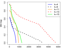
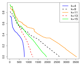
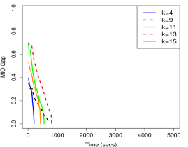

D.2 Lasso, Debiased Lasso and MIO
We present here comparisons of the debiased Lasso with MIO and Lasso.
Debiasing is often used to mitigate the shrinkage imparted by the Lasso regularization parameter. This is done by performing an unrestricted least squares on the support selected by the Lasso. Of course the results will depend upon the tuning parameter used for the problem. We use two methods towards this end. In the first method we find the best Lasso solution (by obtaining an optimal tuning parameter based on minimizing predictive error on a held out validation set); we then obtain the un-regularized least squares solution for that Lasso solution. This typically performed worse than Lasso in all the experiments we tried—see Tables 3 and 4. The unrestricted least squares solution on the optimal model selected by the Lasso (as shown in Figure 4) had worse predictive performance than the Lasso, with the same sparsity pattern, as shown in Table 3. This is probably due to overfitting since the model selected by the Lasso is quite dense compared to . Table 4 presents the results for . We consider the same example presented in Figure 9, Example 1. First of all, Table 4 presents the prediction performance of Lasso after debiasing—we considered the same tuning parameter considered optimal for the Lasso problem. We see that as in the case of Table 3, the debiasing does not lead to improved performance in terms of prediction error.
We thus experimented with another variant of the debiased Lasso, where for every we computed the Lasso solution (2) and obtained by performing an unrestricted least squares fit on the support selected by the Lasso solution at . This method can be thought of delivering feasible solutions for Problem (1), for a value of determined by the Lasso solution at . The success of this method makes a case in support of using criterion (1). The tuning parameter was then selected by minimizing predictive performance on a held out test validation set. This method in general performed better than Lasso in delivering a sparser model with better predictive accuracy than the Lasso. The performance of the debiased Lasso was similar to Sparsenet and was in general inferior to MIO by orders of magnitude, especially for the problems where the pairwise correlations between the variables was large and SNR was low and . The results are presented in Table 5,6 (for the case ) and 7 and 8 (for the case ).
Debiasing at optimal Lasso model,
| SNR | Ratio: Lasso/ Debiased Lasso | |
|---|---|---|
| 6.33 | 0.5 | 0.33 |
| 3.17 | 0.5 | 0.54 |
| 1.58 | 0.5 | 0.53 |
| 6.97 | 0.8 | 0.67 |
| 3.48 | 0.8 | 0.64 |
| 1.74 | 0.8 | 0.63 |
| 8.73 | 0.9 | 1 |
| 4.37 | 0.9 | 0.58 |
| 2.18 | 0.9 | 0.61 |
Debiasing at optimal Lasso model,
| SNR | Ratio: Lasso/Debiased Lasso | |
|---|---|---|
| 10 | 0.8 | 0.90 |
| 7 | 0.8 | 1.0 |
| 3 | 0.8 | 0.91 |
The performance of this model was comparable with Sparsenet—it was better than Lasso in terms of obtaining a sparser model with better predictive accuracy. However, the performance of MIO was significantly better than the debiased version of the Lasso, especially for larger values of and smaller SNR values.
Sparsity of Selected Models,
| SNR | Lasso | Debiased Lasso | MIO | |
| 6.33 | 0.5 | 27.6 (2.122) | 10.9 (0.65) | 10.8 (0.51) |
| 3.17 | 0.5 | 27.7 (2.045) | 10.9 (0.65) | 10.1 (0.1) |
| 1.58 | 0.5 | 28.0 (2.276) | 10.9 (0.65) | 10.2 (0.2) |
| 6.97 | 0.8 | 34.1 (3.60) | 10.4 (0.15) | 10 (0.0) |
| 3.48 | 0.8 | 34.0 (3.54) | 10.9 (0.55) | 10.2 (0.2) |
| 1.74 | 0.8 | 33.7 (3.49) | 13.7 (1.50) | 10 (0.0) |
| 8.73 | 0.9 | 25.9 (0.94) | 13.9 (0.68) | 10.5 (0.17) |
| 4.37 | 0.9 | 34.6 (3.23) | 18.1 (1.30) | 10.2 (0.25) |
| 2.18 | 0.9 | 34.7 (3.28) | 20.5 (1.85) | 10.1 (0.10) |
Predictive Performance of Selected Models,
| SNR | Lasso | Debiased Lasso | MIO | Ratio: | |
| Debiased Lasso/MIO | |||||
| 6.33 | 0.5 | 0.0384 (0.001) | 0.0255 (0.002) | 0.0266 (0.001) | 1.0 |
| 3.17 | 0.5 | 0.0768 (0.003) | 0.0511 (0.004) | 0.0478 (0.002) | 1.0 |
| 1.58 | 0.5 | 0.1540 (0.007) | 0.1021 (0.009) | 0.0901 (0.009) | 1.1 |
| 6.97 | 0.8 | 0.0389 (0.002) | 0.0223 (0.001) | 0.0231 (0.002) | 1.0 |
| 3.48 | 0.8 | 0.0778 (0.004) | 0.0464 (0.003) | 0.0484 (0.004) | 1.0 |
| 1.74 | 0.8 | 0.1557 (0.007) | 0.1156 (0.008) | 0.0795 (0.008) | 1.5 |
| 8.73 | 0.9 | 0.0325 (0.001) | 0.0220 (0.002) | 0.0197 (0.002) | 1.2 |
| 4.37 | 0.9 | 0.0632 (0.002) | 0.0532 (0.003) | 0.0427 (0.008) | 1.3 |
| 2.18 | 0.9 | 0.1265 (0.005) | 0.1254 (0.006) | 0.0703 (0.011) | 1.8 |
We then follow the method described above (for the case), where we consider a sequence of models and find the that delivers the best predictive model on a held out validation set.
Sparsity of Selected Models,
| SNR | Lasso | Debiased Lasso | MIO | |
|---|---|---|---|---|
| 10 | 0.8 | 25.7 (1.73) | 7.9 (0.43) | 5 (0.12) |
| 7 | 0.8 | 27.8 (2.69) | 8.1 (0.43) | 5 (0.16) |
| 3 | 0.8 | 28.0 (2.72) | 10.0 (0.88) | 6 (1.18) |
Predictive Performance of Selected Models,
| SNR | Lasso | Debiased | MIO | Ratio: | |
| Lasso | Debiased Lasso/ MIO | ||||
| 10 | 0.8 | 0.084 (0.004) | 0.046 (0.003) | 0.014 (0.005) | 3.3 |
| 7 | 0.8 | 0.122 (0.005) | 0.070 (0.004) | 0.020 (0.007) | 3.5 |
| 3 | 0.8 | 0.257 (0.012) | 0.185 (0.016) | 0.151 (0.027) | 1.2 |