RCSLenS: Testing gravitational physics through the cross-correlation of weak lensing and large-scale structure

Abstract

The unknown nature of “dark energy” motivates continued cosmological tests of large-scale gravitational physics. We present a new consistency check based on the relative amplitude of non-relativistic galaxy peculiar motions, measured via redshift-space distortion, and the relativistic deflection of light by those same galaxies traced by galaxy-galaxy lensing. We take advantage of the latest generation of deep, overlapping imaging and spectroscopic datasets, combining the Red Cluster Sequence Lensing Survey (RCSLenS), the Canada-France-Hawaii Telescope Lensing Survey (CFHTLenS), the WiggleZ Dark Energy Survey and the Baryon Oscillation Spectroscopic Survey (BOSS). We quantify the results using the “gravitational slip” statistic $E_{G}$, which we estimate as $0.48\pm 0.10$ at $z=0.32$ and $0.30\pm 0.07$ at $z=0.57$, the latter constituting the highest redshift at which this quantity has been determined. These measurements are consistent with the predictions of General Relativity, for a perturbed Friedmann-Robertson-Walker metric in a Universe dominated by a cosmological constant, which are $E_{G}=0.41$ and $0.36$ at these respective redshifts. The combination of redshift-space distortion and gravitational lensing data from current and future galaxy surveys will offer increasingly stringent tests of fundamental cosmology.

1 Introduction

A wide set of cosmological observations suggest that the dynamics of the Universe are currently dominated by some form of “dark energy”, which in standard Friedmann-Robertson-Walker (FRW) models is propelling an acceleration in late-time cosmic expansion (e.g. Planck collaboration 2015a, Aubourg et al. 2015, Betoule et al. 2014). The physical nature of dark energy is not yet understood, and a widely-considered possibility is that the nature of gravitation differs on large cosmological scales from the predictions of General Relativity (GR) in an FRW metric. As a result, a key task for current cosmological surveys is to construct observations to test for such departures.

Gravitational physics produces a rich variety of observable signatures that can be used for this purpose. The most precisely-measured signal results from the “peculiar motions” of galaxies as they fall toward overdense regions as non-relativistic test particles in a perturbed FRW metric. These motions produce correlated Doppler shifts in galaxy redshifts that manifest themselves as an overall anisotropy in the measured clustering signal as a function of the angle to the line-of-sight (Kaiser 1987), known as redshift-space distortion (RSD). The amplitude of this anisotropy has been accurately measured in a number of galaxy surveys across a range of redshifts and allows the growth rate $f$ of cosmic structure, which describes the gravitational amplification of density perturbations, to be inferred. To date, these measurements are broadly consistent with the prediction of the standard cosmological model (e.g. Blake et al. 2011, Beutler et al. 2012, Reid et al. 2012, de la Torre et al. 2013, Samushia et al. 2014).

A highly complementary route for probing gravitational effects is to study the deflections of relativistic test particles such as photons, which are additionally sensitive to the curvature of space produced by density perturbations. These deflections, known as gravitational lensing, may be measured in a statistical sense using the correlations imprinted in the apparent shapes of background galaxies behind foreground lenses in deep imaging surveys. The level of the signal is determined by both the amplitude of the density fluctuations around the lenses (again reflecting the growth of structure with redshift) and the relative distances of the source-lens systems, both of which may be predicted by a given cosmological model (for a review, see Bartelmann & Schneider 2001). Recent projects such as the Canada-France-Hawaii Telescope Lensing Survey (CFHTLenS) have allowed a suite of such tests to be carried out (e.g. Heymans et al. 2013, Simpson et al. 2013) by providing deep, wide, high-resolution imaging.

Zhang et al. (2007) proposed that a powerful gravitational consistency check might be performed by using the same set of galaxies to trace non-relativistic gravitationally-driven motion using redshift-space distortion, and to serve as foreground lenses for probing the relativistic deflection of light from background sources. In this way, it could be ascertained whether the relative amplitude of these two effects, driven by the same underlying density perturbations traced by the lenses, was consistent with the prediction of GR assuming a perturbed FRW metric for a given set of cosmological parameters including the matter density $\Omega_{m}$. This can be achieved by measuring a quantity known as the “gravitational slip” $E_{G}(R)$ as a function of physical scale $R$, which is constructed from the galaxy-galaxy lensing signal and the redshift-space distortion and clustering amplitude of the lenses. Standard perturbed GR cosmology predicts that a scale-independent value $E_{G}=\Omega_{m}/f$ should be recovered. Failure of this cross-check would indicate either the breakdown of linear perturbation theory, an inconsistency in the assumed cosmological parameters such as the matter density or curvature, or that a large-scale modification in gravitational physics was required.

A requirement for carrying out this programme is the availability of galaxy spectroscopic redshift surveys and deep gravitational lensing imaging surveys which overlap on the sky. Reyes et al. (2010) performed this test using data from the Sloan Digital Sky Survey (SDSS) covering $\approx 5000$ deg², using a sample of $\approx 70{,}000$ Luminous Red Galaxy lenses at $z=0.32$ and shape measurements with a surface density $\approx 1$ arcmin^-2 and produced a gravitational slip measurement consistent with GR in a $\Lambda$-dominated Universe. The goal of our current study is to use new, significantly deeper, spectroscopic and imaging survey datasets to extend these tests to higher source densities and more distant redshifts $z\approx 0.6$. In particular we use imaging data from CFHTLenS (Heymans et al. 2012) and the 2nd Red Cluster Sequence Lensing Survey (Gilbank et al. 2011, Hildebrandt et al. 2015), and overlapping spectroscopic data from the WiggleZ Dark Energy Survey (Drinkwater et al. 2010) and Baryon Oscillation Spectroscopic Survey (BOSS, Eisenstein et al. 2011) to carry out this investigation. We note that a measurement of $E_{G}$ using lensing of the Cosmic Microwave Background was recently presented by Pullen et al. (2015).

The structure of our paper is as follows: in Section 2 we introduce the theory underpinning galaxy-galaxy lensing and RSD in a perturbed FRW metric, the methodology for suppressing small-scale information which is difficult to model, and our test statistic for gravitational physics, $E_{G}$. In Section 3 we summarize our input datasets, and in Section 4 we present the galaxy-galaxy lensing measurements expressed as both the average tangential shear as a function of angular separation $\gamma_{t}(\theta)$ and the differential surface density as a function of projected physical separation $\Delta\Sigma(R)$, together with a series of tests for shape-measurement systematics. We pay particular attention to how the full redshift probability distribution of each source, determined from photometric-redshift estimation, can be included in an unbiased estimator of $\Delta\Sigma(R)$ from source-lens pairs. In Section 5 we describe a large set of new N-body simulations, including self-consistent gravitational lensing, that we use for determining errors in our measurements and testing models. Finally in Section 6 we present the first cosmological implications, including new measurements of $E_{G}$ up to redshift $z\approx 0.6$. We conclude in Section 7.

This paper is the first in a series which will dissect the cosmological information in overlapping deep galaxy lensing and spectroscopic datasets. Future studies will present full cosmological fits including Cosmic Microwave Background data in a range of modified gravity scenarios, and the use of photometric-redshift and spectroscopic-redshift cross-correlations to determine simultaneously the source redshift distributions and cosmological parameters.

2 Theory: galaxy-galaxy lensing and redshift-space distortion

2.1 Galaxy-galaxy lensing: tangential shear

Galaxy-galaxy lensing describes the shear-density correlation imprinted between the shapes of background source galaxies and the foreground large-scale structure traced by the lens galaxies; it is measured by computing the azimuthally-averaged tangential shear of the sources as a function of their angular distance $\theta$ from the lenses:

$$\langle\gamma_{t}(\theta)\rangle=\langle\delta_{g}(\vec{x})\,\gamma_{t}(\vec{x}+\vec{\theta})\rangle,$$ (1)

where $\gamma_{t}$ denotes the tangential shear component of the source with respect to the separation vector $\vec{\theta}$ connecting it to the lens, and $\delta_{g}(\vec{x})$ is the overdensity of the lens galaxies at position $\vec{x}$. Fourier transforming the variables in Equation 1 we find that (e.g. Hu & Jain 2004)

$$\langle\gamma_{t}(\theta)\rangle=\frac{1}{2\pi}\int_{0}^{\infty}d\ell\,\ell\,C_{g\kappa}(\ell)\,J_{2}(\ell\theta),$$ (2)

where $J_{2}$ denotes the 2nd-order Bessel function of the first kind, and the galaxy-convergence cross-power spectrum $C_{g\kappa}$ is given by (e.g. Bartelmann & Schneider 2001, Guzik & Seljak 2001, Joachimi & Bridle 2010)

$$C_{g\kappa}(\ell)=\frac{3\Omega_{m}H_{0}^{2}}{2c^{2}}\int_{0}^{\infty}dz\frac{(1+z)}{\chi(z)}P_{gm}\left(\frac{\ell}{\chi},z\right)p_{l}(z)W(z),$$ (3)

where

$$W(z)=\int_{z}^{\infty}dz^{\prime}\,p_{s}(z^{\prime})\left[\frac{\chi(z^{\prime})-\chi(z)}{\chi(z^{\prime})}\right].$$ (4)

In these equations, $\chi(z)$ is the co-moving radial coordinate at redshift $z$ assuming a spatially-flat Universe, $P_{gm}(k,z)$ is the galaxy-mass cross-power spectrum at wavenumber $k$, $[p_{s}(z),p_{l}(z)]$ are the redshift probability distributions of the source and lens samples, normalized such that $\int_{0}^{\infty}p(z)\,dz=1$, and $H_{0}$ and $c$ are Hubble’s constant and the speed of light, respectively. These relations make the approximations of using the Limber equation and neglecting additional effects such as cosmic magnification and intrinsic alignments.

These equations make clear that the tangential shear is sensitive to the cosmological model through the distance-redshift relation describing the relative geometry of the source-lens-observer systems, and through the clustering of the matter overdensities traced by the lenses. Our method of estimating $\langle\gamma_{t}(\theta)\rangle$ from the data is described in Section 4.1.

2.2 Galaxy-galaxy lensing: differential surface density

In this study we are interested in “de-projecting” the angular tangential shear profile in order to recover the statistics of the projected mass surface density $\Sigma$ around the lenses as a function of projected spatial separation $R$. Assuming an axisymmetric lens, and a single lens-source pair with respective redshifts $(z_{l},z_{s})$, the average tangential shear at projected separation $R$ from the lens is given by

$$\langle\gamma_{t}(\theta)\rangle=\frac{\Delta\Sigma(R,z_{l})}{\Sigma_{c}(z_{l},z_{s})}$$ (5)

(e.g. Bartelmann & Schneider 2001), where $\theta=R/\chi(z_{l})$ and the differential projected surface mass density $\Delta\Sigma$ is defined in terms of $\Sigma(R)$ by

$$\Delta\Sigma(R)\equiv\overline{\Sigma}(<R)-\Sigma(R),$$ (6)

where $\overline{\Sigma}(<R)$ is the average mass density within a circle of radius $R$,

$$\overline{\Sigma}(<R)\equiv\frac{2}{R^{2}}\int_{0}^{R}R^{\prime}\,\Sigma(R^{\prime})\,dR^{\prime}.$$ (7)

In Equation 5 the co-moving critical surface mass density $\Sigma_{c}$ is given by

$$\Sigma_{c}(z,z^{\prime})=\frac{c^{2}}{4\pi G}\left\{\frac{\chi(z^{\prime})}{\left[\chi(z^{\prime})-\chi(z)\right]\,\chi(z)\,(1+z)}\right\},$$ (8)

where $G$ is the gravitational constant and $z^{\prime}>z$. The differential projected surface density around the lenses is related to the lens galaxy-matter cross-correlation function $\xi_{gm}(r)$ by

$$\Delta\Sigma(R)=\overline{\rho_{m}}\int_{-\infty}^{\infty}\xi_{gm}(\sqrt{R^{2}+\Pi^{2}})\,d\Pi,$$ (9)

where $\overline{\rho_{m}}$ is the mean cosmological matter density, related to the critical density $\rho_{c}=3H_{0}^{2}/8\pi G=2.77518\times 10^{11}\,h^{2}M_{\odot}$ Mpc^-3 [with $h=H_{0}/(100$ km s^-1 Mpc^-1)] by $\overline{\rho_{m}}=\rho_{c}\,\Omega_{m}$, and $\Pi$ denotes the co-moving line-of-sight separation.

By substituting Equations 3 and 4 into Equation 2, and comparing with the result of substituting Equations 8 and 9 into Equation 5, we can determine after some algebra how Equation 5 generalizes for broad source and lens distributions. The result is

$$\langle\gamma_{t}(\theta)\rangle=\int_{0}^{\infty}dz\,p_{l}(z)\,\Delta\Sigma(R,z)\int_{z}^{\infty}dz^{\prime}\,p_{s}(z^{\prime})\frac{1}{\Sigma_{c}(z,z^{\prime})},$$ (10)

noting that for narrow lens and source redshift distributions, $p_{l}(z)=\delta_{D}(z-z_{l})$ and $p_{s}(z)=\delta_{D}(z-z_{s})$, Equation 10 reduces to Equation 5.

Equation 10 clarifies that for a broad lens redshift distribution it is not possible to solve for $\Delta\Sigma(R,z_{l})$ in closed form. However, for a narrow lens redshift distribution, averaging over a background source redshift distribution $p_{s}(z)$, we can recover the relation

$$\Delta\Sigma(R,z_{l})\approx\langle\gamma_{t}(\theta)\rangle\left[\int_{z_{l}}^{\infty}dz^{\prime}\,p_{s}(z^{\prime})\frac{1}{\Sigma_{c}(z_{l},z^{\prime})}\right]^{-1}.$$ (11)

Section 4.2 presents an analysis to justify that this approximation is acceptable, given the source and lens redshift distributions of our datasets. Our method of estimating $\Delta\Sigma(R)$ from the data is described in Section 4.2.

2.3 Galaxy clustering and redshift-space distortion

The cross-power spectrum of lens galaxies and underlying mass that appears in Equation 3, $P_{gm}$, and the equivalent cross-correlation function in Equation 9, $\xi_{gm}$, depend on the manner or “bias” with which the lens galaxies trace the matter field. Although this bias is in general a stochastic, non-linear and scale-dependent function, it may be approximated on sufficiently-large scales as a linear mapping between the galaxy and matter overdensity, $\delta_{g}(\vec{x})=b\,\delta_{m}(\vec{x})$ (e.g., Scherrer & Weinberg 1998). In this case $\xi_{gm}(r)=b\,\xi_{mm}(r)$, in terms of the matter auto-correlation function $\xi_{mm}(r)$ which may be modelled from the cosmological parameters, where the unknown bias parameter $b$ may be determined using the auto-correlation function of the lenses, $\xi_{gg}(r)=b^{2}\,\xi_{mm}(r)$.

Since 3D measurements of galaxy clustering are performed in redshift-space, the apparent radial positions of the galaxies contain an additional correlated imprint from galaxy peculiar velocities, known as redshift-space distortion (RSD). In particular, the Fourier transform of the redshift-space galaxy overdensity field, $\tilde{\delta}_{g}^{s}$, is given under certain assumptions (e.g. Percival & White 2009, Blake et al. 2011) by

$$\tilde{\delta}_{g}^{s}(k,\mu)=\tilde{\delta}_{g}(k)-\mu^{2}\,\tilde{\theta}(k),$$ (12)

where $\tilde{\theta}(k)$ is the Fourier transform of the divergence of the peculiar velocity field in units of the co-moving Hubble velocity and $\mu$ is the cosine of the angle of the Fourier mode to the line-of-sight.

Assuming that the velocity field is generated under linear perturbation theory then $\tilde{\theta}(k)=-f\,\tilde{\delta}_{m}(k)$, where $f$ is the growth rate of structure, expressible in terms of the growth factor $D(a)$ at cosmic scale factor $a$ as $f\equiv d\ln{D}/d\ln{a}$. The growth factor is defined in terms of the amplitude of a single perturbation as $\delta(a)=D(a)\,\delta(1)$. Under the assumption of linear galaxy bias we then obtain the standard expression for the redshift-space galaxy power spectrum in linear theory (Kaiser 1987)

$$P_{gg}^{s}(k,\mu)=b^{2}\,(1+\beta\mu^{2})^{2}\,P_{mm}(k),$$ (13)

where we have introduced the redshift-space distortion parameter $\beta=f/b$, which governs the amplitude of the measured RSD.

The anisotropic imprint of RSD in galaxy clustering allows the measurement of the gravitational growth rate and, consequently, powerful tests of gravitational physics. However, it also introduces an extra amplitude factor in the relation between $\xi_{gg}$ and $\xi_{mm}$, complicating inferences about the galaxy bias. In order to avoid this issue the real-space “projected” correlation function $w_{p}(R)$, independent of RSD, can instead be constructed by integrating the 3D galaxy correlation function $\xi_{gg}(R,\Pi)$ along the line-of-sight:

$$w_{p}(R)=\int_{-\infty}^{\infty}\xi_{gg}(R,\Pi)\,d\Pi.$$ (14)

Our method of estimating $w_{p}(R)$ from the data is described in Section 6.1. In practice the limits of Equation 14 must be taken as large, finite values.

2.4 Suppressing small-scale information

Equation 6 demonstrates that the amplitude of $\Delta\Sigma(R)$ depends on the surface density of matter around galaxies across a range of smaller scales from zero to $R$. This is problematic from the viewpoint of fitting cosmological models to the data since at small scales, within the halo virial radius, the cross-correlation coefficient between the matter and galaxy fluctuations is a complex function which is difficult to predict from first principles (Baldauf et al. 2010, Mandelbaum et al. 2010). In order to remove this sensitivity to small-scale information these authors proposed a new statistic, the annular differential surface density (ADSD), denoted by $\Upsilon$ and defined by

$$\Upsilon_{gm}(R,R_{0}) = \Delta\Sigma(R)-\frac{R_{0}^{2}}{R^{2}}\,\Delta\Sigma(R_{0})$$ (15)

$$= \frac{2}{R^{2}}\int_{R_{0}}^{R}R^{\prime}\,\Sigma(R^{\prime})\,dR^{\prime}$$

$$- \Sigma(R)+\frac{R_{0}^{2}}{R^{2}}\Sigma(R_{0}),$$

which does not contain information originating from scales $R<R_{0}$. The small-scale limit $R_{0}$ is chosen to be large enough to reduce the main systematic effects discussed above, but small enough to preserve a high signal-to-noise ratio in the measurements (also see the discussion in Mandelbaum et al. 2013). An alternative approach is to model the halo occupation statistics and marginalize over the free parameters (e.g., Cacciato et al. 2013).

The corresponding quantity suppressing the small-scale contribution to the galaxy auto-correlations is

$$\Upsilon_{gg}(R,R_{0})=\rho_{c}$$

$$\left[\frac{2}{R^{2}}\int_{R_{0}}^{R}R^{\prime}\,w_{p}(R^{\prime})\,dR^{\prime}-w_{p}(R)+\frac{R_{0}^{2}}{R^{2}}w_{p}(R_{0})\right].$$ (16)

We assume $R_{0}=1.5\,h^{-1}$ Mpc as our fiducial value following Reyes et al. (2010), and demonstrate in Section 6.3 that our results are insensitive to this choice.

2.5 Testing gravitational physics: the $E_{G}$ statistic

In general scalar theories of gravity, the perturbed FRW spacetime metric $ds^{2}$ may be expressed in terms of the Newtonian potential $\Psi$ and curvature potential $\Phi$:

$$ds^{2}=\left[1+2\,\Psi(\vec{x},t)\right]\,c^{2}\,dt^{2}-a(t)^{2}\left[1-2\,\Phi(\vec{x},t)\right]\,d\vec{x}^{2}.$$ (17)

Relativistic particles, such as photons experiencing gravitational lensing, collect equal contributions from these two potentials as they traverse spacetime, such that their equations of motion (and hence the resulting lensing patterns) are determined by $\nabla^{2}(\Psi+\Phi)$. However, the motion of non-relativistic particles arising from the gravitational attraction of matter, which produces galaxy clustering and RSD, is sensitive only to the derivatives of the Newtonian potential $\nabla^{2}\Psi$ (e.g., Jain & Zhang 2008).

In standard General Relativity (GR), in the absence of anisotropic stress, $\Psi(\vec{x},t)=\Phi(\vec{x},t)$ and both potentials are related to the matter overdensity via the Poisson equation $\nabla^{2}\Phi=4\pi Ga^{2}\overline{\rho_{m}}\delta_{m}$. Therefore, by measuring if both the gravitational lensing of photons and galaxy peculiar velocity respond in an identical manner to the matter overdensity traced by the lens galaxies in our datasets, we can perform a fundamental test of whether the relation between $(\Psi+\Phi)$ and $\Psi$ follows the GR expectation (assuming this perturbation approximation applies).

Zhang et al. (2007) proposed that this test can be efficiently carried out by cross-correlating lens galaxies to both the surrounding velocity field using RSD and to the shear of background galaxies using galaxy-galaxy lensing. In particular, Reyes et al. (2010) implemented this consistency test by constructing the “gravitational slip” statistic

$$E_{G}(R)=\frac{1}{\beta}\frac{\Upsilon_{gm}(R,R_{0})}{\Upsilon_{gg}(R,R_{0})},$$ (18)

which is independent of both the galaxy bias factor $b$ and the underlying amplitude of matter clustering $\sigma_{8}$, given that $\beta\propto 1/b$, $\Upsilon_{gm}\propto b\,\sigma_{8}^{2}$ and $\Upsilon_{gg}\propto b^{2}\,\sigma_{8}^{2}$. The perturbed GR model prediction on large scales is then a scale-independent quantity $E_{G}=\Omega_{m}/f$ (see Leonard et al. (2015) for a more detailed discussion of this approximation). We measure $E_{G}$ and carry out this consistency test in Section 6.3. We note that a failure of this consistency check does not necessarily indicate evidence for gravitational physics beyond GR: other possible explanations would include a breakdown in validity of linear perturbation theory, or that the value of $\Omega_{m}$ or curvature differs from that predicted by measurements of the Cosmic Microwave Background radiation.

3 Data

Figure 1: (R.A., Dec.) distribution in the Northern Galactic Pole (NGP) and Southern Galactic Pole (SGP) of the datasets used in this analysis: the BOSS DR10 galaxy sample (black dots), the WiggleZ survey regions (red rectangles), the CFHTLenS fields (green rectangles) and the RCSLenS fields (blue rectangles).

Table 1: Statistics for CFHTLenS and RCSLenS fields cross-correlated with WiggleZ and BOSS data. The effective (unmasked) areas are shown for the full source field, the pointings which contain a minimum of four filters such that photometric redshifts are available, and the pointings which overlap with the lens distribution (where two values are quoted for this latter area, they refer to WiggleZ/BOSS). The effective weighted source density as computed by Equation 19 is listed as $n_{\rm eff}$. The number of lenses contained in the overlapping areas of WGZLoZ, WGZHiZ, LOWZ and CMASS are displayed as $N_{\rm WGZLoZ}$, $N_{\rm WGZHiZ}$, $N_{\rm LOWZ}$ and $N_{\rm CMASS}$, respectively. Some fields have overlap with both WiggleZ and BOSS lens samples, which would result in potentially correlated measurements. In such cases the lens sample producing the lower signal-to-noise measurement, indicated with an asterisk, is excluded from the analysis.

Field	$A_{\rm eff}$[all]	$A_{\rm eff}$[photo-$z$]	$A_{\rm eff}$[overlap]	$n_{\rm eff}$	$N_{\rm WGZLoZ}$	$N_{\rm WGZHiZ}$	$N_{\rm LOWZ}$	$N_{\rm CMASS}$
	[deg2]	[deg2]	[deg2]	[arcmin-2]
CFHTLS W1	56.0	56.0	48.7	14.0	-	-	1998	3856
CFHTLS W4	17.6	17.6	17.6	13.1	-	-	832	1711
RCS 0047	51.8	37.2	37.2	5.4	3029∗	4343∗	2273	3735
RCS 0133	25.0	13.3	13.3	4.5	-	-	646	1236
RCS 0310	60.9	52.3	52.3	4.9	4249	6140	-	-
RCS 1303	12.9	8.3	3.7	5.3	-	-	128	412
RCS 1514	60.0	30.4	5.8/30.4	5.7	152∗	448∗	1504	3337
RCS 1645	22.8	20.1	20.1	6.7	-	-	1098	2008
RCS 2143	65.5	47.1	47.1	5.7	7190∗	8752∗	2337	4718
RCS 2329	36.0	32.1	19.0/32.1	6.4	494∗	882∗	1356	3122
RCS 2338	57.3	19.5	19.5	4.9	1336	2158	-	-

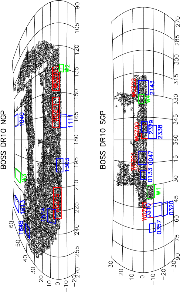
We perform this test of gravitational physics by utilizing the overlap of lensing measurements from two imaging surveys, the Canada-France-Hawaii Telescope Lensing Survey (CFHTLenS; Heymans et al. 2012) and the Red Cluster Sequence Lensing Survey (RCSLenS, Hildebrandt et al. 2015), with two spectroscopic-redshift large-scale structure surveys, the WiggleZ Dark Energy Survey (Drinkwater et al. 2010) and the Baryon Oscillation Spectroscopic Survey (BOSS, Eisenstein et al. 2011). Figure 1 displays the sky distribution of the CFHTLenS, RCSLenS, WiggleZ and BOSS datasets used in this analysis, and the surveys and source selection are briefly described in the sub-sections below.

A total of 11 CFHTLenS and RCSLenS survey fields overlap with the WiggleZ and BOSS DR10 data, comprising a total area of 466 deg² (74 deg² for CFHTLenS and 392 deg² for RCSLenS). Table 1 lists some statistics for these fields, including the total effective (unmasked) field area, the area for which the available imaging allows photometric redshifts to be derived, the subset of that area which overlaps with the lens distributions, the effective source density (defined below) and the number of lenses in each of the overlapping spectroscopic surveys used in the analysis, where the BOSS data is split into the LOWZ and CMASS samples (described below). The RCSLenS fields used for cross-correlation with (WiggleZ, BOSS) contain an overlapping photo-$z$ area of (72, 184) deg². The CFHTLenS fields used for cross-correlation with BOSS cover 74 deg².

Our datasets enable us to construct five distinct source-lens survey pairings: RCSLenS-WiggleZ, RCSLenS-LOWZ, RCSLenS-CMASS, CFHTLenS-LOWZ and CFHTLenS-CMASS. We split the WiggleZ lenses into two independent redshift bins, $0.15<z<0.43$ (“WGZLoZ”) and $0.43<z<0.7$ (“WGZHiZ”), which coincide with the redshift ranges of LOWZ and CMASS, respectively, producing a total of six possible pairings. In the analyses that follow we will often present separate measurements for these six cases, optimally combining the measurements in each individual field using inverse-variance weighting.

3.1 CFHTLenS

The CFHTLenS is a deep multi-colour survey optimized for weak lensing analyses, observed as part of the Canada-France-Hawaii Telescope (CFHT) Legacy Survey in five optical bands $u^{*}g^{\prime}r^{\prime}i^{\prime}z^{\prime}$ using the 1 deg² camera MegaCam. The data span four fields, two of which (W1 and W4) overlap with the spectroscopic-redshift data used in this analysis. The main lensing analysis is performed on $i^{\prime}$ band data, for which the observations have a $5\sigma$ point-source limiting magnitude $i^{\prime}\approx 25.5$. The imaging data are processed with THELI (Erben et al. 2013), galaxy ellipticities are measured by the Bayesian model-fitting software lensfit (Miller et al. 2013), and photometric redshifts are derived from PSF-matched photometry (Hildebrandt et al. 2012) using the Bayesian photometric redshift code BPZ (Benitez 2000). Additive and multiplicative shear calibration corrections have been derived as a function of galaxy size and signal-to-noise (Heymans et al. 2012, Miller et al. 2013). The survey pointings have been subjected to a stringent cosmology-independent systematic-error analysis (Heymans et al. 2012), as a result of which a subset of around $25\%$ of the pointings have been flagged as possessing potential systematic errors. Given that galaxy-galaxy lensing is much less sensitive than cosmic shear to such systematics due to the circular averaging over lens-source pairs, as thoroughly investigated for CFHTLenS by Velander et al. (2014), we do not remove these pointings from our analysis. We explicitly checked that any difference in the galaxy-galaxy lensing statistics between these choices was within the range of statistical fluctuations.

The lensfit pipeline returns measured ellipticity components $(e_{1},e_{2})$ for each source, together with an approximately optimal weight $w^{s}$, a combination of the variance in the intrinsic ellipticity and the measurement error due to photon noise (Miller et al. 2013). We note that the sign of $e_{2}$ listed in the source catalogues must be reversed in our cross-correlation pipeline, because the positive $x$-direction of pixel coordinates lies in the negative R.A. direction. We cut the catalogue to sources with weights $w^{s}>0$ which lie in unmasked areas of data. No magnitude cuts are applied, although fainter galaxies are downweighted by lower values of $w^{s}$. We also do not apply a star-galaxy separation cut, since stars are already assigned negligible weights by lensfit. The effective source density for lensing analyses (following Heymans et al. 2012) is defined by

$$n_{\rm eff}=\frac{1}{A_{\rm eff}}\,\frac{\left(\sum_{i}w^{s}_{i}\right)^{2}}{\sum_{i}(w^{s}_{i})^{2}},$$ (19)

where $A_{\rm eff}$ is the effective (unmasked) area. The values derived for (W1, W4) are $n_{\rm eff}=(14.0,13.1)$ arcmin^-2. (We note that Chang et al. 2013 provide another possible definition of $n_{\rm eff}$.)

The BPZ photometric-redshift pipeline returns a full redshift probability distribution $p_{\rm BPZ}(z)$ for each source, binned in intervals of $\Delta z=0.05$ in the range $0<z<3.5$, and we make use of this full information when computing the lensing signal. For purposes of binning sources in photo-$z$ slices, we use the maximum-likelihood redshift value $z_{B}$ of these distributions. The source redshift distribution $p_{s}(z)$, which is required for cosmological modelling and for building the mock catalogues below, is constructed by stacking the $p_{\rm BPZ}(z)$ distributions for each source, weighting by the lensfit weights,

$$p_{s}(z)\propto\sum_{i}w^{s}_{i}\,p_{{\rm BPZ},i}(z)$$ (20)

We do not apply any photo-$z$ cuts in our fiducial analysis, and demonstrate that our results are insensitive to such cuts.

We note that Miyatake et al. (2015) and More et al. (2015) recently presented related galaxy-galaxy lensing measurements for CFHTLenS-CMASS, with the aim of understanding the properties of the dark matter haloes traced by the lenses, and performing joint cosmological and halo occupation model fits.

3.2 RCSLenS

The 2nd Red Sequence Cluster Survey (RCS2, Gilbank et al. 2011) is a nearly 800 deg² imaging survey in three optical bands $g^{\prime}r^{\prime}z^{\prime}$ carried out with the CFHT. The primary survey area is divided into 13 well-separated patches on the sky, each with an area ranging from 20 to 100 deg². Nine of these fields (with properties listed in Table 1) overlap with the spectroscopic-redshift data used in this analysis. The main lensing analysis is performed using the $r^{\prime}$ band data, with limiting magnitude $r^{\prime}\approx 24.3$. Around two-thirds of the RCS2 area has also been imaged in the $i^{\prime}$ band.

The RCS2 team have presented a series of investigations of galaxy-galaxy lensing using these data, probing the occupation and shapes of dark matter halos (van Uitert et al. 2011, 2012, Cacciato et al. 2014) and the connection to galaxy luminosity, stellar mass and velocity dispersion (van Uitert et al. 2013, 2015). We focus instead on cosmological applications of this dataset.

The RCSLenS dataset is a lensing re-analysis of the RCS2 imaging data constructed by applying the same processing pipeline for shape measurement and photometric-redshift estimation as developed for CFHTLenS (Hildebrandt et al. 2015). The effective RCSLenS source density derived using Equation 19, $n_{\rm eff}\approx 5.5$ arcmin^-2, is lower than the corresponding value for CFHTLenS due to the shallower imaging, but the data cover a significantly wider area. BPZ photometric redshifts are only derived for pointings containing 4 optical bands $g^{\prime}r^{\prime}i^{\prime}z^{\prime}$, which correspond to about two-thirds of the survey area (with statistics for individual fields listed in Table 1). We note that the absence of $u^{*}$ band imaging in RCSLenS causes slightly larger photo-$z$ errors and a greater outlier fraction at low redshifts, owing to more serious colour-redshift degeneracies.

The RCSLenS shape catalogues have been subject to a “blinding” process to prevent confirmation bias in analysis (Hildebrandt et al. 2015, see also Kuijken et al. 2015 for a full description of the same process). In brief, the catalogues contain four sets of ellipticity data, one of which is the true data, whilst the other three sets have been manipulated by a trusted external colleague by different amounts unknown to the science team, sufficient to prevent confirmation bias but not so extreme as to render those data suspiciously discrepant. All scientific analyses are repeated for each of the 4 blindings. Once the results are ready for publication, the blinding key is provided by the external, after which the science team can make no further undocumented modifications to analysis procedures.

3.3 WiggleZ Dark Energy Survey

The WiggleZ Dark Energy Survey (Drinkwater et al. 2010) is a large-scale galaxy redshift survey of bright emission-line galaxies over the redshift range $z<1$ with median redshift $z\approx 0.6$, which was carried out at the Anglo-Australian Telescope at Siding Spring, Australia, between August 2006 and January 2011. In total, of order $200{,}000$ redshifts were obtained, covering of order 1000 deg² of equatorial sky divided into seven well-separated regions, labelled as (00, 01, 03, 09, 11, 15, 22) by their location on the sky in hours of R.A.

WiggleZ galaxies were selected for observation using colour and magnitude cuts from a combination of optical and UV imaging. The optical imaging employed was from the SDSS in the Northern Galactic Pole and from the RCS2 survey in the Southern Galactic Pole, spanning a total of 6 RCS2 fields (0047, 0310, 1514, 2143, 2329, 2338). The WiggleZ dataset is therefore very well-suited for providing lenses for cross-correlation with RCSLenS sources. The 0047, 1514, 2143 and 2329 fields are also covered by BOSS, producing higher signal-to-noise galaxy-galaxy lensing measurements in these cases, and therefore to avoid the complication of the covariance we focus on analyzing the 2 remaining fields, 0310 and 2338. When measuring the galaxy-galaxy lensing signal, we also cut the lens and source distributions to the subset of MegaCam pointings containing both lenses and sources (the “overlap area”) listed in Table 1. After these cuts, we used a total of $5{,}585$ WGZLoZ lenses and $8{,}298$ WGZHiZ lenses in our analysis. The WiggleZ lens selection function within each region was determined using the methods described by Blake et al. (2010). The average galaxy bias factor of the WiggleZ lenses is $b\approx 1$.

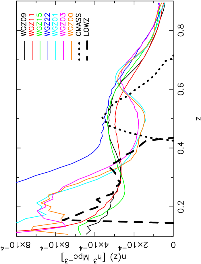
Figure 2 plots the number density distribution with redshift of the WiggleZ lens samples in the different survey regions. The typical number density is $n\approx 3\times 10^{-4}\,h^{3}$ Mpc^-3 at the effective redshift $z\approx 0.6$, with a tail to lower number densities at high redshift ($1\times 10^{-4}\,h^{3}$ Mpc^-3 at $z\approx 0.9$) and higher number densities at low redshift ($6\times 10^{-4}\,h^{3}$ Mpc^-3 at $z\approx 0.1$). Some variation amongst WiggleZ regions is evident, due to differences in the colour/magnitude selection and completeness of the spectroscopic follow-up (for full details, see Drinkwater et al. 2010).

Figure 2: Number density distribution with redshift of lenses in each WiggleZ survey region and in the BOSS LOWZ/CMASS samples. The redshift distribution differs between WiggleZ regions because of varying colour/magnitude selection and completeness of spectroscopic follow-up.

3.4 BOSS

BOSS is a spectroscopic follow-up survey of the SDSS III imaging survey (Eisenstein et al. 2011), which has obtained redshifts for over a million galaxies covering $10{,}000$ deg². All observations have been carried out at the Sloan Telescope located at Apache Point Observatory in New Mexico. BOSS uses colour and magnitude cuts to select two classes of galaxies to be targetted for spectroscopy, the “LOWZ” sample which contains red galaxies at $z<0.43$ and the “CMASS” sample which is designed to be approximately stellar-mass limited for $z>0.43$. We use the data catalogues provided by the SDSS 10th Data Release (DR10); full details of these catalogues are given by Eisenstein et al. (2011), Dawson et al. (2013) and Anderson et al. (2014).

Following the practice of the BOSS science papers we cut the LOWZ sample to $0.15<z<0.43$ and the CMASS sample to $0.43<z<0.7$, in order to avoid redshift overlap and create homogeneous galaxy samples. The redshift distributions of these samples are shown in Figure 2 and are comparable to the WiggleZ dataset. The galaxy bias factors of the LOWZ and CMASS samples are $b\approx 1.6$ and $b\approx 1.9$, respectively (Chuang et al. 2014, Sanchez et al. 2014), hence these objects are significantly more clustered than WiggleZ galaxies.

In order to correct for the effects of redshift failures, fibre collisions and other known systematics affecting the angular completeness (correlated with the stellar density and seeing), BOSS galaxies are assigned completeness weights (as specified in Equation 18 of Anderson et al. 2014). We included these weights in our determination of the auto-correlation function of the galaxies, but they do not affect the galaxy-galaxy lensing measurements because they are uncorrelated with the background shapes.

Figure 3: Measurements of $\gamma_{t}(\theta)$ (left column) and $\gamma_{\times}(\theta)$ (right column) for the cross-correlation of different combinations of source-lens datasets. We show results for both the data (black solid circles) and mock mean (red open circles), with the errors based on measurements for a set of 374 mock catalogues. The overplotted model is the expectation for the mock mean based on the input cosmology of the simulations. $\chi^{2}$ statistics are quoted for the $\gamma_{\times}$ measurements with respect to a model of zero, with number of degrees of freedom ${\rm dof}=20$.

As noted in Table 1, the BOSS sample overlaps 2 CFHTLenS fields (W1 and W4) and 7 RCSLenS fields (0047, 0133, 1303, 1514, 1645, 2143, 2329). We utilized a total of $12{,}172$ LOWZ lenses and $24{,}135$ CMASS lenses in our analysis.

4 Galaxy-galaxy lensing measurements

In this Section we describe our estimation of the stacked tangential shear around the lenses as a function of angular separation and the differential surface density around the lenses as a function of the projected physical separation. In the latter case we use the full source photometric-redshift probability distribution when computing the lensing signal.

4.1 Average tangential shear $\gamma_{t}(\theta)$

The ellipticity components $(e_{1,i},e_{2,i})$ of source $i$ relative to the positive $x$-axis are defined by

$$(e_{1},e_{2})=\left(\frac{r-1}{r+1}\right)(\cos{2\psi},\sin{2\psi}),$$ (21)

where $\psi$ is the position angle of a galaxy with axial ratio $r$ measured anti-clockwise from the positive $x$-axis. These ellipticity components can be rotated to new values $[e_{t}(i,j),e_{\times}(i,j)]$ relative to a line connecting source $i$ and lens $j$ by

$$e_{t}(i,j)=-e_{1,i}\cos{2\phi(i,j)}-e_{2,i}\sin{2\phi(i,j)}$$ (22)

and

$$e_{\times}(i,j)=e_{1,i}\sin{2\phi(i,j)}-e_{2,i}\cos{2\phi(i,j)},$$ (23)

where $\phi(i,j)$ is the angle of the line connecting source $i$ and lens $j$ to the positive $x$-axis (in the range $-90^{\circ}<\phi<90^{\circ}$). Our galaxy-galaxy lensing estimators for the tangential shear $\gamma_{t}$ and cross shear $\gamma_{\times}$ are then:

$$\gamma_{t}(\theta)=\frac{\sum_{{\rm sources}\,i}\sum_{{\rm lenses}\,j}w^{s}_{i}\,w^{l}_{j}\,e_{t}(i,j)\,\Theta(i,j)}{\sum_{{\rm sources}\,i}\sum_{{\rm lenses}\,j}w^{s}_{i}\,w^{l}_{j}\,\Theta(i,j)}$$ (24)

and

$$\gamma_{\times}(\theta)=\frac{\sum_{{\rm sources}\,i}\sum_{{\rm lenses}\,j}w^{s}_{i}\,w^{l}_{j}\,e_{\times}(i,j)\,\Theta(i,j)}{\sum_{{\rm sources}\,i}\sum_{{\rm lenses}\,j}w^{s}_{i}\,w^{l}_{j}\,\Theta(i,j)},$$ (25)

where $w^{s}_{i}$ is the lensfit weight of source $i$, $w^{l}_{j}$ is the weight of lens galaxy $j$ which we set to the completeness weights for BOSS galaxies and $w^{l}=1$ for WiggleZ galaxies (since in that case the completeness is incorporated in the random catalogues), $\Theta(i,j)$ is equal to 1 if the angular separation between source $i$ and lens $j$ lies in bin $\theta$ and equal to 0 otherwise, and the sums are taken over unique pairs. We performed measurements in 20 logarithmically-spaced angular bins from $\theta=0.01^{\circ}$ to $1^{\circ}$. Multiplicative shear bias corrections are computed and applied as discussed in Section 4.3. The cross shear $\gamma_{\times}$ should be consistent with zero signal for weak gravitational lensing but potentially non-zero for distortions due to systematic errors.

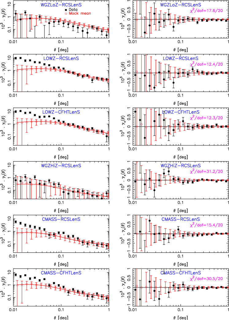
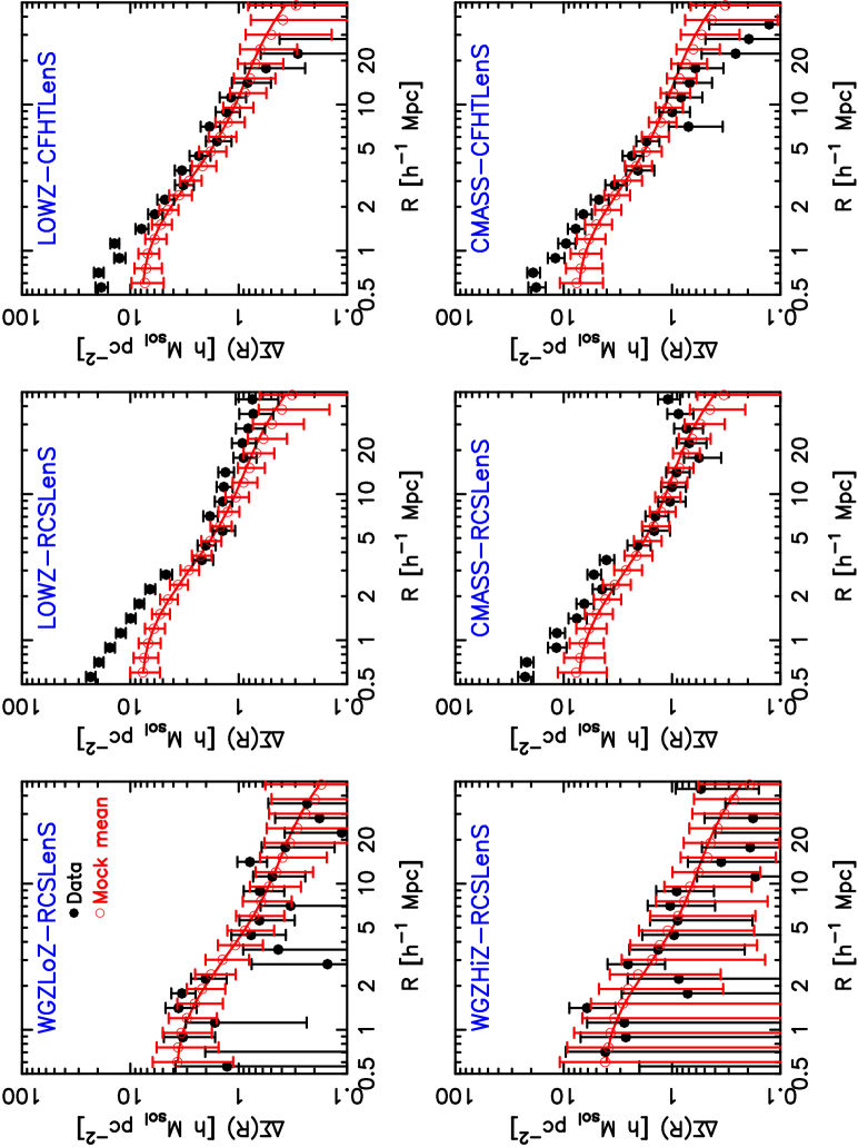
Figure 3 shows the resulting measurements of the tangential and cross shear for the six different combinations of source-lens datasets. The measurements are performed in the individual fields listed in Table 1 and then combined together using inverse-variance weighting. The errors in the measurements are obtained by applying the same analysis pipeline to a set of 374 mock catalogues, which are constructed by the process described in Section 5, and appropriately scaling the standard deviation of the mock statistics. In Figure 3 we plot measurements for both the data (black solid circles) and the mean of the mock catalogues (red open circles), where the solid line is the model prediction for the mocks based on the input cosmology of the simulations. In the absence of systematic effects, the cross shear should be consistent with zero. Values of the chi-squared statistic are shown for each source-lens combination, determined for a model $\gamma_{\times}=0$ using the covariance matrix built from the mock catalogues. Our measurements are consistent with this expectation.

At small scales, for values of $\theta$ corresponding to projected physical separations $R<2\,h^{-1}$ Mpc, the amplitude of galaxy-galaxy lensing in the mock falls below that measured in the data. This arises because of halo occupation effects on small scales particularly affecting Luminous Red Galaxies; it presents no concern for our analysis, in which physical effects originating at small scales $R<R_{0}$ are explicitly suppressed.

4.2 Differential surface density $\Delta\Sigma(R)$

In Section 2.2 we demonstrated that for a relatively narrow lens distribution, $\Delta\Sigma(R,z_{l})$ could be estimated from the tangential galaxy shear via Equation 11, which we re-write here as

$$\Delta\Sigma(R,z_{l})=\gamma_{t}(\theta)/\left(\overline{\Sigma_{c}^{-1}}\right),$$ (26)

where

$$\overline{\Sigma_{c}^{-1}} \equiv \int_{z_{l}}^{\infty}dz_{s}\,p_{s}(z_{s})\,\Sigma_{c}^{-1}(z_{l},z_{s})$$ (27)

$$= \frac{4\pi G\,(1+z_{l})\,\chi(z_{l})}{c^{2}}\int_{z_{l}}^{\infty}dz_{s}\,p_{s}(z_{s})\left[1-\frac{\chi(z_{l})}{\chi(z_{s})}\right].$$

We implemented this calculation for each lens-source pair by using the source photometric-redshift probability distribution, $p_{s}(z)=p_{\rm BPZ}(z)$. Therefore we estimate $\Delta\Sigma$ using only that lensing data for which photometric-redshift information is available, as listed in Table 1.

Figure 4: $\Delta\Sigma(R)$ measured for the cross-correlation of different combinations of source-lens datasets. We show results for the data and the mock mean. The overplotted model is included only for comparison with the mock mean.

Figure 5: A comparison of the measurements of $\Delta\Sigma(R)$ for different combinations of source-lens datasets using the approximate estimator of Equation 30 based only on the best source photometric redshift $z_{B}$, plotted as the solid (black) circles, and the unbiased estimator of Equation 28, based on the full redshift probability distribution $p_{\rm BPZ}(z)$ of each source, plotted as the open (magenta) circles. For the purposes of this plot the errors were determined by jack-knife re-sampling.

For our determinations of $\overline{\Sigma_{c}^{-1}}$ using Equation 27, and conversions of source-lens angular separations $\theta$ to projected separations $R=\theta\,\chi(z_{l})$, we adopted a fiducial flat $\Lambda$CDM cosmological model with matter density $\Omega_{m}=0.27$. Our motivation for this choice, which is in better agreement with the fits to the Cosmic Microwave Background fluctuations using WMAP satellite data (Komatsu et al. 2011) rather than the later Planck satellite data (Planck collaboration 2015b), is to ensure consistency with the fiducial cosmological model adopted for the RSD analyses of the WiggleZ and BOSS data (Blake et al. 2011, Sanchez et al. 2014), which would be subject to Alcock-Paczynski distortion in different models. Adopting the higher value of $\Omega_{m}$ preferred by the Planck analysis would not produce a significant change in our measurements compared to the statistical errors.

When averaging the estimates of Equation 26 over the lens-source pairs, each source must now be inverse-variance weighted as $w^{s}\left(\overline{\Sigma_{c}^{-1}}\right)^{2}$ and hence our final estimator is

$$\Delta\Sigma(R)=\frac{\sum_{{\rm sources}\,i}\sum_{{\rm lenses}\,j}w^{s}_{i}\,w^{l}_{j}\,\overline{\Sigma_{c}^{-1}}_{ij}\,e_{t}(i,j)\,\Theta(i,j)}{\sum_{{\rm sources}\,i}\sum_{{\rm lenses}\,j}w^{s}_{i}\,w^{l}_{j}\,\left[\overline{\Sigma_{c}^{-1}}_{ij}\right]^{2}\,\Theta(i,j)}$$ (28)

(see also Miyatake et al. 2015). This estimator corrects for the dilution in lensing signal caused by the non-zero probability that a source is situated in front of the lens, $z_{s}<z_{l}$.

We note that an approximate version of this estimator has been used in previous studies where only the maximum-likelihood source redshift $z_{s}$ is available, rather than the full probability distribution $p_{s}(z_{s})$. In this approximation the lens-source pairs are restricted to those cases for which $z_{s}>z_{l}$ and the differential surface density for each pair is estimated as

$$\Delta\Sigma(R,z_{l})\approx\gamma_{t}(\theta)\,\Sigma_{c}(z_{l},z_{s}).$$ (29)

The inverse-variance weight of each source-lens pair is now $w^{s}\,\Sigma_{c}^{-2}$ such that the approximate estimator reads

$$\Delta\Sigma(R)=\frac{\sum_{{\rm sources}\,i}\sum_{{\rm lenses}\,j}w^{s}_{i}\,w^{l}_{j}\,\Sigma_{c,ij}^{-1}\,e_{t}(i,j)\,\Theta(i,j)}{\sum_{{\rm sources}\,i}\sum_{{\rm lenses}\,j}w^{s}_{i}\,w^{l}_{j}\,\Sigma_{c,ij}^{-2}\,\Theta(i,j)}.$$ (30)

This relation will contain a bias as far as $\Sigma_{c}\neq 1/\overline{\Sigma_{c}^{-1}}$, although that bias can be corrected through comparison with spectroscopic catalogues (Nakajima et al. 2012).

Figure 4 shows the measurement of $\Delta\Sigma(R)$ using Equation 28 in 20 logarithmically-spaced bins in $R$ from $0.5$ to $50\,h^{-1}$ Mpc, for the six different combinations of source-lens datasets, displaying results for both the data and the mock mean. As above, the errors in these measurements are obtained using the 374 mock catalogues introduced in Section 5. Our choice of this binning scheme allows us to search for scale-dependence in the measurement whilst retaining good signal-to-noise in each bin.

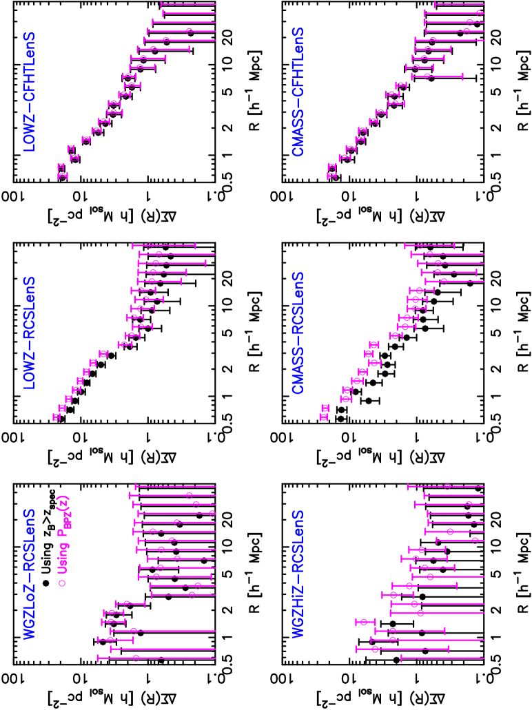
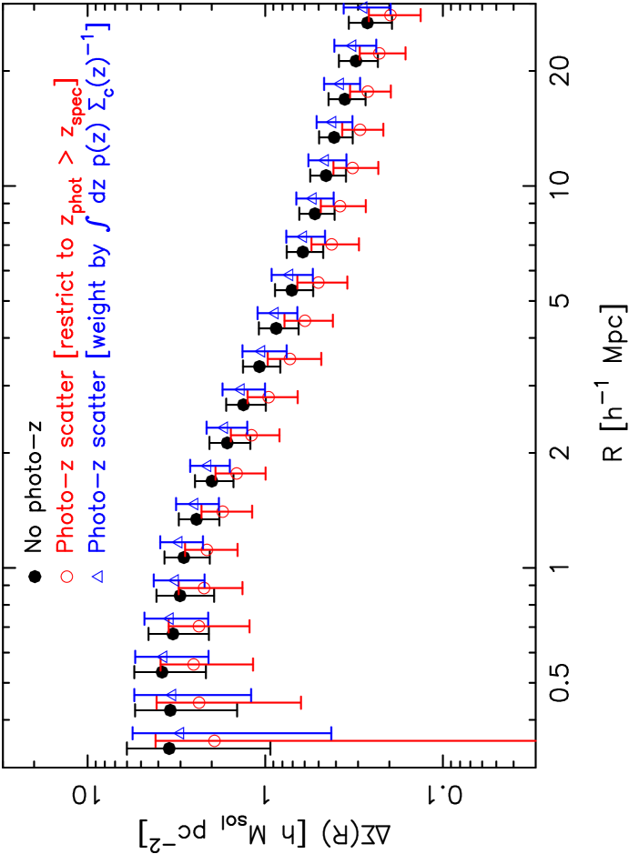
We now consider in more detail the difference in results produced by the unbiased estimator of Equation 28 and the approximate estimator of Equation 30. First, Figure 5 compares measurements of $\Delta\Sigma(R)$ using the two estimators. We conclude that the approximate estimator contains a significant systematic bias, especially when using photometric redshifts with precision characteristic of the RCSLenS data. Secondly, Figure 6 presents a verification of our successful recovery of $\Delta\Sigma(R)$ in the presence of photometric-redshift errors, using the mock catalogues described in Section 5. A toy photo-$z$ model is applied to the mock catalogues, in which redshifts are scattered in accordance with a Gaussian distribution of zero mean and standard deviation $0.2\times(1+z)$, and the differential surface density is then estimated using both Equation 28 and Equation 30. The measurements in which the full source redshift probability distributions are used agree well with an analysis in which the photo-$z$ scatter is not applied.

Figure 6: Verification that the estimator of Equation 28 successfully recovers the input value of $\Delta\Sigma(R)$ in mock catalogues. A toy photo-$z$ model is applied to the mocks, in which redshifts are scattered in accordance with a Gaussian distribution of zero mean and standard deviation $0.2\times(1+z)$. The differential surface density is then estimated using both Equation 30, restricting the calculation to source-lens pairs for which $z_{\rm phot}>z_{\rm spec}$ (red open circles), and Equation 28, which uses the full information of the photo-$z$ probability distribution (green open triangles). These determinations are compared to the measurements without application of photometric redshifts (black solid circles). In all cases the mock mean is plotted, where the error represents the standard deviation of the mocks.

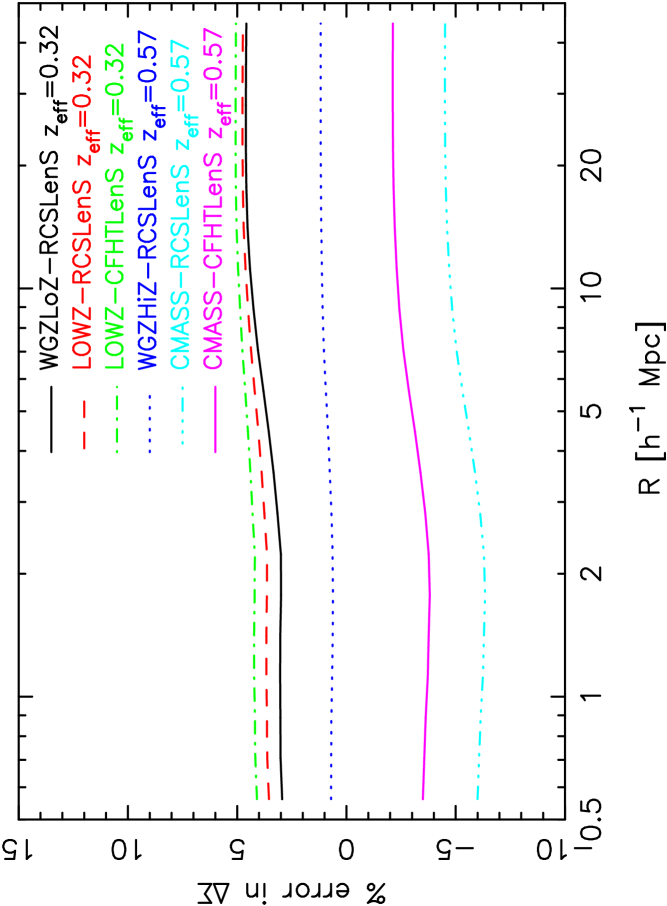
Finally, Figure 7 assesses how accurately the narrow lens approximation described in Section 2.2 holds for the specific lens and source redshift distributions of our samples. The amplitude of the systematic error is calculated by comparing the value of $\Delta\Sigma(R)$ that would be inferred at the effective redshifts at which RSD is measured for the different lens samples by substituting Equation 10 in Equation 11, with the fiducial value of $\Delta\Sigma(R)$ evaluated using Equation 9. We find that the resulting amplitude of the systematic error in $\Delta\Sigma$ (and consequently $E_{G}$) is about $5\%$, which is significantly smaller than the statistical error in $E_{G}$ of around $20\%$. We conclude that the narrow-lens approximation is acceptable for our analysis.

Figure 7: The systematic error in determination of $\Delta\Sigma$ that results in the application of the narrow-lens approximation of Equation 11 at the effective redshift of the RSD measurements of each lens sample.

We note (without further calculation) an additional issue for estimating $E_{G}$ that could occur for wide lens redshift slices. The weighting applied to each source-lens pair when estimating $\Delta\Sigma(R)$, $\overline{\Sigma_{c}^{-1}}$, contains a dependence on the lens redshift which may induce a systematic difference in the relative weighting of lens galaxies to that used in the measurement of their projected auto-correlation function $w_{p}(R)$, which would become important if the bias of the lenses evolved across the redshift slice. However, the bias of both WiggleZ and BOSS lenses is a fairly flat function of redshift across these ranges (Blake et al. 2009, Anderson et al. 2014).

4.3 Calibration and random-catalogue corrections

Figure 8: The cross-correlation between shapes and random lenses, $\Delta\Sigma_{\rm rand}(R)$, measured for the different combinations of source and lens samples. The results are averaged over 40 random catalogues. A jack-knife error is plotted, noting that this error is only accurate for small scales and is a significant over-estimate for the largest scales. This systematic correction is subtracted from the data, which is standard practice for calibrating galaxy-galaxy lensing measurements (see for example Mandelbaum et al. 2005).

Bias in ellipticity measurements may be described by a linear combination of a multiplicative error $m$ and an additive error $c$ such that

$$e_{i}^{\rm obs}=(1+m_{i})\,e_{i}^{\rm true}+c_{i}+{\rm Noise},$$ (31)

where $i=1,2$ denotes the two ellipticity components.

Velander et al. (2014) show that the additive shear bias has a negligible effect for galaxy-galaxy lensing measurements with CFHTLenS data. We follow the standard practice of performing this calibration by subtracting the correlation with a random lens catalogue as described below, which represents an empirical calculation of any additive shear residual.

The multiplicative shear bias correction $m$ defined in Equation 31 has been modelled for lensfit processing of MegaCam data using a shear recovery test based on galaxy image simulations as a function of source signal-to-noise $SN$ and size in pixels $r$:

$$m(SN,r)=\frac{\beta}{{\rm log}_{10}(SN)}\exp{(-r\,SN\,\alpha)},$$ (32)

where $\alpha=0.057$ and $\beta=-0.37$ (Miller et al. 2013). The same correction applies to both $e_{1}$ and $e_{2}$, and is greater for sources with smaller signal-to-noise ratios and sizes. We propagated this correction into the measurement of $\gamma_{t}(\theta)$ by evaluating

$$K(\theta)=\frac{\sum_{{\rm sources}\,i}\sum_{{\rm lenses}\,j}w_{i}^{s}\,w_{j}^{l}\,m_{i}\,\Theta(i,j)}{\sum_{{\rm sources}\,i}\sum_{{\rm lenses}\,j}w_{i}^{s}\,w_{j}^{l}\,\Theta(i,j)},$$ (33)

such that the corrected measurement is given by

$$\gamma_{t}^{\rm corrected}(\theta)=\frac{\gamma_{t}^{\rm uncorrected}(\theta)}{1+K(\theta)}.$$ (34)

We note that this multiplicative shear bias correction must be applied in a global fashion, not on an individual source basis, due to its correlation with the measured source ellipticity values owing to its dependence on $SN$ and $s$ in Equation 32.

The analogous formula for the correction to be applied to $\Delta\Sigma(R)$ is

$$K(R)=\frac{\sum_{{\rm sources}\,i}\sum_{{\rm lenses}\,j}w^{s}_{i}\,w^{l}_{j}\,m_{i}\,\Sigma_{c,ij}^{-1}\,\Theta(i,j)}{\sum_{{\rm sources}\,i}\sum_{{\rm lenses}\,j}w^{s}_{i}\,w^{l}_{j}\,\Sigma_{c,ij}^{-2}\,\Theta(i,j)}.$$ (35)

Equation 35 assumes that we are using the approximate estimator of Equation 30; when instead employing the unbiased estimator of Equation 28 we should replace $\Sigma_{c,ij}^{-1}$ by $\overline{\Sigma_{c}^{-1}}_{ij}$. Figure 20 in Appendix A.2 displays the corrections measured for the different source and lens samples; we find that $K\approx-0.06$ independent of scale, such that the amplitude of the galaxy-galaxy lensing signal must be boosted by $\approx 6\%$.

The shear estimated by these methods might still be contaminated by two further effects: (1) large-scale residual shape-measurement systematics, such as an imperfectly-modelled optical distortion across the camera field; (2) the physical association of source and lens galaxies, for example sharing the same dark matter halo, diluting the cross-correlation signal since these sources will not be lensed and yet may have been scattered to higher redshifts by photo-$z$ error. The importance of both of these effects can be determined using random lenses sampled from the same selection function as the data, where we averaged over 40 random catalogues in these analyses (checking that our final results were insensitive to the number of catalogues and the uncertainty in the correction).

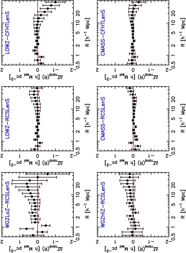
First, we re-ran the shear measurement replacing the data lenses with the random lens catalogues. The result for the differential projected surface density, which we denote $\Delta\Sigma_{\rm rand}(R)$, is displayed in Figure 8 as the combined signals for the different combinations of source and lens samples. In the absence of residual coherent tangential distortions the signal should be consistent with zero; however, a significant correction is obtained at large scales for some of our samples, in particular CFHTLenS, and is always subtracted from our measurements of $\Delta\Sigma(R)$. We investigate the effect of physically-associated sources in Appendix A.5, concluding that it is not significant for the scales we study. We compared our results to those presented by Miyatake et al. (2015). These authors find a more significant large-scale signal in $\Delta\Sigma_{\rm rand}(R)$ for CMASS-CFHTLenS than we do, although we note that they analyze a different geometry of CMASS lenses.

4.4 Summary of systematics tests

We supported our science measurements with a series of tests for potential systematic errors. These results are described in detail in the Appendices, and we provide a brief summary in this Section.

In Appendix A.1 we present a series of systematics tests based on re-measuring $\gamma_{t}(\theta)$ following various manipulations of the shear catalogue:

• Rotation of the sources by $45^{\circ}$ (i.e., $e_{1,{\rm new}}=e_{2,{\rm old}}$ and $e_{2,{\rm new}}=-e_{1,{\rm old}}$).

• Randomizing the shear values amongst the source catalogue.

• Replacing the lens catalogue by a random catalogue.

The results of these tests are consistent with $\gamma_{t}=0$, as expected.

Systematic errors in the BPZ photometric redshift distributions would imprint errors in the determination of $\Delta\Sigma(R)$ (given that these full probability distributions are used in the measurement, as described above). In order to search for such effects we performed a “scaling test” of the galaxy-galaxy lensing signal measured for the same set of foreground lenses using background sources in a series of different photo-$z$ slices spanning the range $0<z_{B}<1.6$. The results are detailed in Appendix A.3. We find that a consistent lens singular isothermal sphere velocity dispersion is obtained for all source photo-$z$ slices with the possible exception of $0<z_{B}<0.2$, which comprises a negligible number of galaxies. As a final test, we repeated the $E_{G}$ measurement using sources in different $z_{B}$ ranges; these results are discussed in Section 6.3 and demonstrate that the measurement is robust to these choices.

Another potential source of systematic error is intrinsic alignment of the source population with respect to the foreground lenses (Blazek et al. 2012), which is expected to preferentially diminish the average tangential shear of red source galaxies. In Appendix A.4 we carry out shear measurements for red and blue sub-samples to verify that the amplitude of these effects are below the level that would impact our results; we will demonstrate this explicitly in Section 6.3 by repeating the $E_{G}$ measurement for a blue sub-sample.

In addition to the systematic tests carried out in the paper, we refer the reader to Kuijken et al. (2015) who apply the same data analysis software used in this analysis to data from the Kilo Degree Survey.

5 Simulations

Figure 9: Comparison of the mean of various clustering and lensing statistics measured for the mock catalogues, with the expectations based on the input cosmological model of the simulation and the source and lens redshift distributions and bias factors. Results are shown for the lens and source auto-correlation functions $w_{\rm lens}$ and $w_{\rm source}$, the cross-correlation function $w_{\rm source-lens}$, the cosmic shear statistics $\xi_{+}$ and $\xi_{-}$, and the galaxy-galaxy lensing signal $\gamma_{t}$. The error bars correspond to the standard deviation across the mock catalogues (which do not contain shape noise).

5.1 Mock catalogues

In order to test our analysis pipeline and estimate the covariance matrix of the measurements, we created mock catalogues of each source and lens field. These catalogues were built from a set of 374 N-body simulations created using methods similar to those described by Harnois-Deraps, Vafaei & van Waerbeke (2012). In brief, the N-body simulations are produced by the CUBEP³M code with a transfer function obtained from CAMB (Lewis, Challinor & Lasenby  2000) using the following cosmological parameter set: matter density $\Omega_{m}=0.2905$, baryon density $\Omega_{b}=0.0473$, Hubble parameter $h=0.6898$, spectral index $n_{s}=0.969$ and normalization $\sigma_{8}=0.826$. The box-size of the simulations is $L=505\,h^{-1}$ Mpc; this is significantly larger than the simulation set used for modelling the earlier CFHTLenS measurements [$L=(147,231)\,h^{-1}$ Mpc] such that the new simulation set is much less affected by suppression of the large-scale variance by finite box size. For each simulation the density field is output at 18 snapshots, and a survey cone spanning 60 deg² is constructed by pasting together these snapshots, where the division between adjacent snapshots is taken as the mid-point of the cosmic distances corresponding to the output redshifts. The two-component shear fields are also computed at each output redshift, by ray-tracing through the survey cone using Born’s approximation. More details are provided by Harnois-Deraps & van Waerbeke (2015).

For every different survey region and lens-source survey pairing, we converted each simulation line-of-sight into a mock catalogue by generating:

• A source distribution with the surface density values given in Table 1 (adjusted for each region), using the RCSLenS or CFHTLenS source redshift distribution as appropriate, and Monte-Carlo sampling sources from the density field with bias $b_{\rm source}=1$. The source shear components are assigned by linearly interpolating the shear fields at the source redshift from the enclosing lens planes.

• A lens distribution with the numbers given in Table 1 (adjusted for each region), using the average WiggleZ, LOWZ or CMASS redshift distribution as appropriate, sampled from the density fields with bias factors $b_{\rm lens}=(1.0,1.6,1.9)$ for WiggleZ, LOWZ and CMASS, matching the bias measurements of Blake et al. 2010, Chuang et al. 2014 and Sanchez et al. 2014, respectively.

Sources and lenses are produced with a continuous distribution in redshift by interpolating across the finite redshift width of each simulation snapshot; at this stage the angular selection function is uniform across the 60 deg² cone. For a given bias factor $b$, the galaxy density field $\rho_{g}$ is related to the mass density field $\rho_{m}$ as

$$\frac{\rho_{g}}{\langle\rho_{g}\rangle}=1+b\left[\frac{\rho_{m}}{\langle\rho_{m}\rangle}-1\right].$$ (36)

We note that a bias model with $b>1$ cannot be applied self-consistently on all scales because then $\rho_{g}$ contains negative regions. We avoid these regions by imposing the condition $\rho_{g}={\rm max}(\rho_{g},0)$, which reduces the effective value of the large-scale bias by a few per cent (we settled on this approach after experimenting with various approaches for ameliorating this effect such as smoothing the density field before applying the sub-sampling).

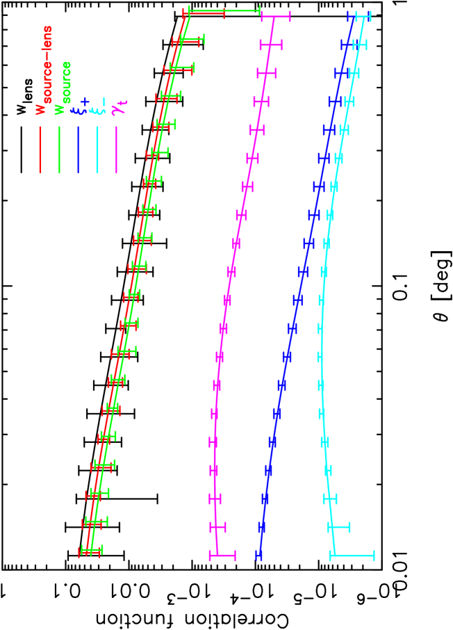
Figure 9 tests the resulting mock catalogues by measuring the average tangential shear $\gamma_{t}$, cosmic shear signal $(\xi_{+},\xi_{-})$ and source-lens auto- and cross- angular correlation functions $w(\theta)$ for the RCSLenS-WiggleZ mock catalogues (prior to the application of shape noise). The lines are the model predictions assuming the input cosmological parameters of the simulation, and source and lens redshift distributions and bias factors. The matter power spectrum is generated using the CAMB transfer function with non-linear contribution from HALOFIT (Smith et al. 2003). The mock mean closely follows the model predictions in each case.

Shape noise is applied to the source catalogues using the following method:

• A complex noise $n=n_{1}+n_{2}\,i$ is formed for each source, where $n_{1}$ and $n_{2}$ are drawn from Gaussian distributions with standard deviation $\sigma_{e}$.

• A complex shear $\gamma=\gamma_{1}+\gamma_{2}\,i$ is formed from the shear components $(\gamma_{1},\gamma_{2})$ obtained from the ray-traced shear field at the source position, linearly interpolating between the values at adjacent snapshot redshifts.

• A complex noisy shear is then determined as $e=(\gamma+n)/(1+n\,\gamma^{*})$ (Seitz & Schneider 1997). The components of the observed shear $(e_{1},e_{2})$ are then found as $e=e_{1}+e_{2}\,i$.

We used the value $\sigma_{e}=0.29$ for our mocks, which is representative of the two imaging surveys (Heymans et al. 2013, Hildebrandt et al. 2015) albeit slightly on the conservative side. The result of this procedure is 374 mock catalogues, matching the global properties of the source and lens samples with a uniform angular selection function across 60 deg².

Figure 10: Comparison of the errors in $\Delta\Sigma(R)$ determined by jack-knife re-sampling of the data (labelled Data JK), by using the 374 simulation lines-of-sight and scaling by an effective area factor (comparing jack-knife re-sampling of the simulations labelled Sim+scale JK, and the scatter between the realizations labelled Sim+scale real), and by generating 149 simulations of each region including the full selection functions (comparing jack-knife re-sampling labelled Sim+mask JK, and the realization scatter labelled Sim+mask real).

Figure 11: Covariance matrices of the $\Delta\Sigma(R)$ measurements for different combinations of source-lens datasets, determined using the scatter across the 374 simulation lines-of-sight. The covariance matrix $C_{ij}$ is displayed as a correlation matrix $C_{ij}/\sqrt{C_{ii}C_{jj}}$.

We also constructed mock catalogues for each survey region including the full survey mask of sources and lenses, implemented by stitching together multiple simulation lines-of-sight and sub-sampling the result to match the survey selection functions. 149 independent mock catalogues for each survey region could be generated from the 374 simulations. This masked simulation set allows the importance of the survey selection function in the measurement error to be determined, as described in the next sub-section.

5.2 Determination of the covariance matrix

We compared several techniques for obtaining errors in the measurement of $\gamma_{t}(\theta)$ and $\Delta\Sigma(R)$:

• Data jack-knife errors, where 16 (4 $\times$ 4) jack-knife regions of typical dimension $\sim 2^{\circ}$ are used per lensing survey region, obtained by dividing the source distribution into sub-samples containing equal number of galaxies using constant R.A. and Dec. boundaries.

• Simulated errors not including the survey mask. We used the simulations discussed above, which comprise 374 lines-of-sight each covering 60 deg². We measured the cross-correlations for each line-of-sight, and scaled the resulting scatter by $\sqrt{(60\,{\rm deg}^{2})/A_{\rm eff}}$ where $A_{\rm eff}$ is the effective (unmasked) area of each source region listed in Table 1.

• Simulated errors including the survey mask, implemented by stitching together multiple lines-of-sight for the simulations and sub-sampling the result to match the selection functions of the sources and the lenses, as discussed above. We measured the cross-correlations for each of the resulting 149 mock catalogues per region; the standard deviation of these measurements constitutes our error estimate.

• Jack-knife errors applied to both types of mock catalogues. For the mocks without the survey mask, we scaled the resulting scatter by $\sqrt{(60\,{\rm deg}^{2})/A_{\rm eff}}$ for each region.

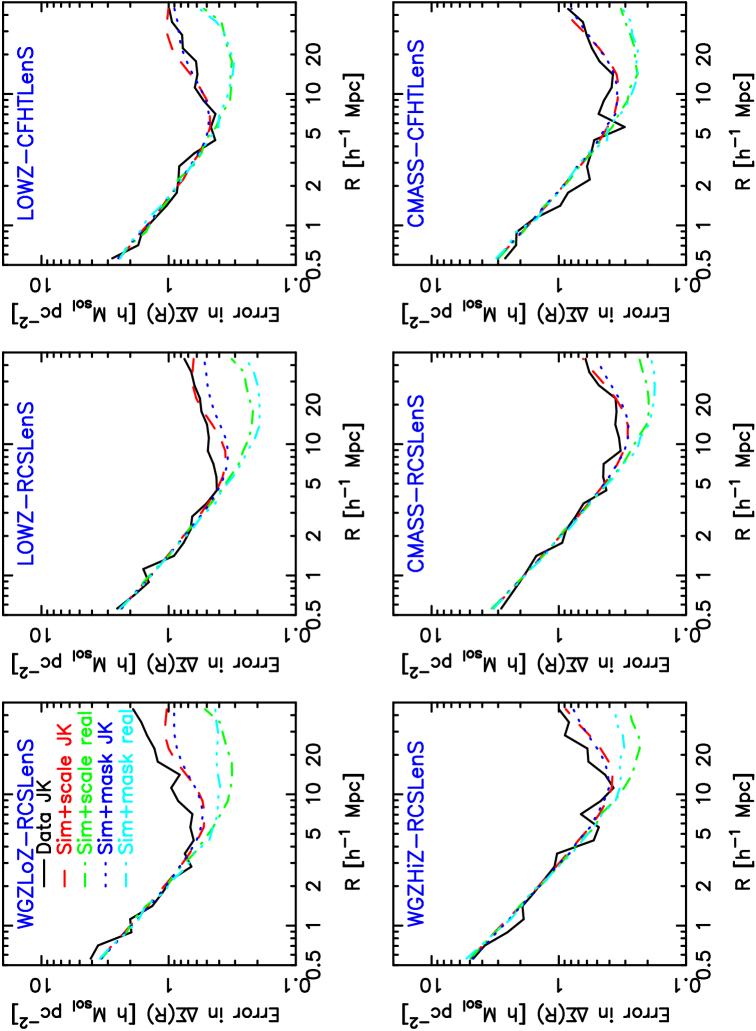
Figure 10 compares these error determinations for the $\Delta\Sigma(R)$ statistic for the different combinations of source-lens datasets, combining results in the different survey regions. The interpretation of these results is that on small scales, the errors in the measurements are dominated by shape noise. At larger scales other effects become important, such as the same source galaxies contributing to many stacks around different lenses, and the “sample variance” contributed by the particular realization of large-scale structure within our lens samples.

All the different error estimates agree well for scales $R<5\,h^{-1}$ Mpc for the low-redshift lenses $(0.15<z<0.43)$ and $R<8\,h^{-1}$ Mpc for the high-redshift lenses $(0.43<z<0.7)$, following a scaling of the projected separation corresponding to a given angular separation. The jack-knife method applied to the simulations produces an error estimate which matches on all scales that obtained from the actual data. The error determined from the area-scaled unmasked simulations and fully-masked simulations matches for all angles, suggesting that the survey mask is of secondary importance for determining the measurement errors compared to the total unmasked area. However, these simulation errors are somewhat lower than the jack-knife errors for larger separations. We expect the jack-knife errors to become unreliable for large scales as the jack-knife regions become increasingly less independent.

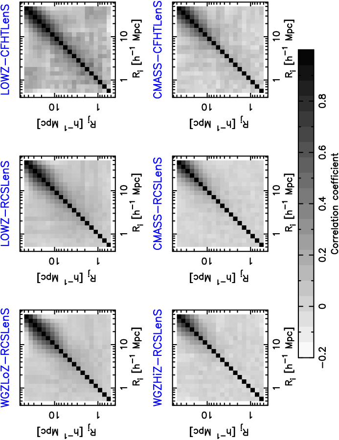
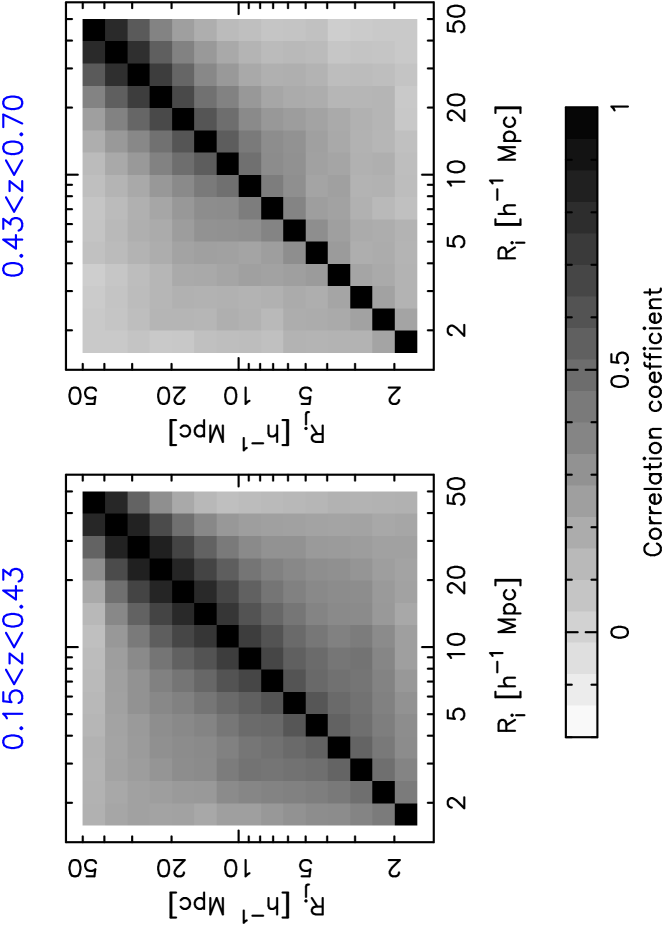
As a result of these tests, we constructed our measurement errors using the ensemble of $N_{\rm real}=374$ mock catalogues without the survey mask. Figure 11 illustrates the off-diagonal elements of the resulting covariance matrix of the $\Delta\Sigma(R)$ statistic for the different combinations of source-lens datasets, constructed as

$${\rm Cov}[\Delta\Sigma(R_{i}),\Delta\Sigma(R_{j})]=\frac{1}{N_{\rm real}-1}\times$$

$$\left[\sum_{k=1}^{N_{\rm real}}\Delta\Sigma^{k}(R_{i})\,\Delta\Sigma^{k}(R_{j})-\overline{\Delta\Sigma(R_{i})}\;\overline{\Delta\Sigma(R_{j})}\right],$$ (37)

where $\Delta\Sigma^{k}$ is measured for the $k$th mock catalogue, and $\overline{\Delta\Sigma(R_{i})}\equiv\sum_{k=1}^{N_{\rm real}}\Delta\Sigma^{k}(R_{i})/N_{\rm real}$. Significant correlations between bins are evident for $R>10\,h^{-1}$ Mpc.

The inverse of these covariance matrices is used in the parameter fits described below. We correct the inverse covariance for the bias due to its maximum-likelihood estimation (Hartlap et al. 2007) via multiplication by the factor

$$\alpha=\frac{N_{\rm real}-N_{\rm bin}-2}{N_{\rm real}-1},$$ (38)

where $N_{\rm bin}$ is the number of data bins used in the fit. For our analyses, $N_{\rm bin}/N_{\rm real}\approx 0.05$.

6 Cosmological results

6.1 Projected galaxy auto-correlation function $w_{p}(R)$

We measured the 2D galaxy correlation function $\xi_{gg}(R,\Pi)$ of each lens sample, binning galaxy pairs by projected separation $R$ and line-of-sight separation $\Pi$. We hence determined the projected correlation functions

$$w_{p}(R)=2\,\sum_{{\rm bins}\,i}\xi_{gg}(R,\Pi_{i})\,\Delta\Pi_{i},$$ (39)

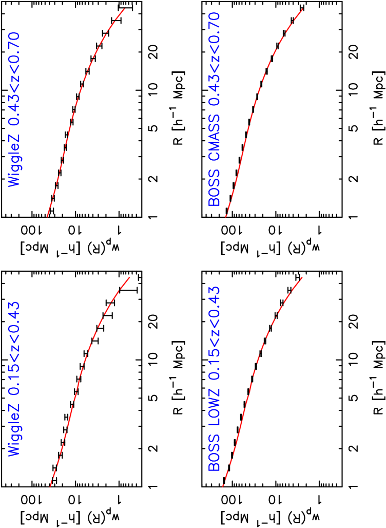
where we summed over 10 logarithmically-spaced bins in $\Pi$ from $0.1$ to $60\,h^{-1}$ Mpc. The measurements of $w_{p}(R)$ in 20 logarithmically-spaced bins in $R$ from $0.5$ to $50\,h^{-1}$ Mpc for the different lens samples are plotted in Figure 12, including jack-knife errors. These projected correlation function measurements are used for simple parameter fits in Section 6.2, and to determine the $E_{G}$ statistic in Section 6.3.

Figure 12: The projected correlation function $w_{p}(R)$ for the different lens data samples used in our analysis. Jack-knife errors are plotted, together with the best-fitting model using both the $w_{p}(R)$ and $\Delta\Sigma(R)$ measurements.

6.2 Measurements of $\sigma_{8}$

Figure 13: The posterior probability distributions of the $\sigma_{8}$ parameter, after marginalizing over the bias factors of the lens galaxies, for the different combinations of source-lens datasets. We also show the probability distribution of the fit to all datasets.

As an initial consistency test of the best-fitting cosmological parameters in the $\Lambda$CDM model, we fitted the measurements of $\Delta\Sigma(R)$ and $w_{p}(R)$ for each source-lens combination varying just $\sigma_{8}$ and the galaxy bias of each lens sample, fixing the other cosmological parameters at the values used to construct the N-body simulations listed in Section 5. Given that $\Delta\Sigma\propto b\,\sigma_{8}^{2}$ and $w_{p}\propto b^{2}\,\sigma_{8}^{2}$, the degeneracy between these normalization parameters is broken and they can be separately determined. Fits were performed using the full covariance matrix of $\Delta\Sigma(R)$ determined from the mock catalogues, and a diagonal error matrix for $w_{p}(R)$ using jack-knife errors. The use of the latter is not significant: the signal-to-noise of $w_{p}(R)$ is much higher than that of $\Delta\Sigma(R)$, and the limiting factor for the final parameter error is the noise in $\Delta\Sigma$, given the initial degeneracy between $b$ and $\sigma_{8}$.

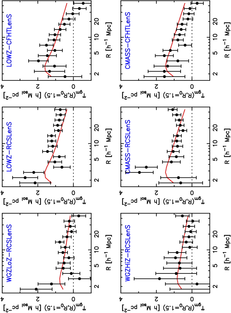
We calculated model predictions using Equation 9 for $\Delta\Sigma(R)$ and Equation 14 for $w_{p}(R)$ and fit to the measurements over the range of scales $R>5\,h^{-1}$ Mpc (noting that our results do not depend significantly on the choice of minimum fitted scale). The best-fitting models to the data are overplotted in Figures 12 and 14. The value of the chi-squared statistic for the best-fitting model is $\chi^{2}=128.3$ for 113 degrees of freedom, indicating a good fit.

Figure 14: The annular differential surface density statistic for the galaxy-mass cross-correlation, $\Upsilon_{gm}(R,R_{0})$, measured for the different combinations of lens-source datasets assuming $R_{0}=1.5\,h^{-1}$ Mpc. We also plot the best-fitting model for each cross-correlation using both the $w_{p}(R)$ and $\Delta\Sigma(R)$ measurements. The errors are based on measurements for a set of 374 mock catalogues. The horizontal dotted line marks $\Upsilon_{gm}=0$.

Figure 15: $E_{G}(R)$ measurements in two independent redshift bins $0.15<z<0.43$ and $0.43<z<0.7$, after combining the results from the different cross-correlations. In the former case, the measurements of Reyes et al. (2010) are plotted as the open circles for comparison. The horizontal solid lines are the prediction of standard gravity, $E_{G}=\Omega_{m}/f$, for our fiducial model $\Omega_{m}=0.27$. The horizontal dotted lines indicate the 1-$\sigma$ variation that would result given $\Delta\Omega_{m}=0.02$, which is indicative of both the WMAP and Planck error in determining this parameter. We note that the data points are correlated, with a covariance matrix displayed in Figure 16.

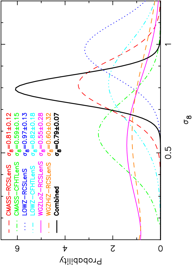
The combined measurement is $\sigma_{8}=0.79\pm 0.07$ consistent with the latest determinations from the Planck satellite (Planck collaboration 2015b). Combining the separate fits to determine the normalizations in two independent redshift bins, $0.15<z<0.43$ (WGZLoZ, LOWZ) and $0.43<z<0.7$ (WGZHiZ, CMASS), we determine $\sigma_{8}(z=0.32)=0.75\pm 0.08$ and $\sigma_{8}(z=0.57)=0.54\pm 0.07$.

In Figure 13 we display the posterior probability distributions of $\sigma_{8}$ for each source-lens dataset, marginalized over the bias factors. The datasets offer roughly comparable constraining power, with CMASS-RCSLenS and WGZHiZ-RCSLenS producing the most and least accurate determinations, respectively.

As a cross-check of the methodology we performed the same fits to the $\Delta\Sigma(R)$ measurements from the mock catalogues for all the combinations of source-lens datasets, using the full-survey realizations including masks. The average parameter measurement across the realizations is $\sigma_{8}=0.80\pm 0.03$ with average value of $\chi^{2}/{\rm dof}=50.5/47$, compared to the input parameter value $\sigma_{8}=0.826$. The slight offset of the fit to lower values than the input is due to the artificial reduction in the clustering amplitude of high-bias mocks constructed via Equation 36, as discussed in Section 5. For $b=1$ mocks we recover the input cosmology within the statistical error in the mean.

Future work will perform a full cosmological parameter analysis of these lensing and clustering datasets, in combination with the CMB.

6.3 Measurement of gravitational slip $E_{G}(R)$

In this Section we use the measured galaxy-galaxy lensing cross-correlations, in combination with the clustering strength and redshift-space distortion properties of the lenses, to compute the scale-dependent $E_{G}$ statistic defined in Equation 18 and hence carry out a test of gravitational physics. We calculated $E_{G}(R)$ for each different combination of source-lens datasets, and then combined the $E_{G}$ measurements in two independent redshift bins, $0.15<z<0.43$ (WGZLoZ, LOWZ) and $0.43<z<0.7$ (WGZHiZ, CMASS).

Firstly we converted the measurements of $\Delta\Sigma(R)$ and $w_{p}(R)$ for each source-lens combination into the annular differential statistics $\Upsilon_{gm}(R)$ and $\Upsilon_{gg}(R)$ defined by Equations 15 and 16, respectively. We determined the values of $\Delta\Sigma(R_{0})$ and $w_{p}(R_{0})$ via a power-law fit to the appropriate statistic, taking the fitting range as $R_{0}/3<R<3R_{0}$. Following Reyes et al. (2010) we assumed a fiducial value $R_{0}=1.5\,h^{-1}$ Mpc for our analysis, although we also consider a range of other choices between $1$ and $3\,h^{-1}$ Mpc. We propagated the errors in $\Delta\Sigma(R_{0})$ and $w_{p}(R_{0})$ into the errors in $\Upsilon_{gm}(R)$ and $\Upsilon_{gg}(R)$, although this source of error is negligible except when $R\approx R_{0}$. We determined the integral appearing in the first term of Equation 16 using a spline fit to the measured $w_{p}(R)$ (noting that these details make a negligible contribution to error propagation). Measurements of $\Upsilon_{gm}(R,R_{0}=1.5\,h^{-1}{\rm Mpc})$ are displayed in Figure 14 for the different source and lens combinations.

We cross-checked the errors in the determination of $\Upsilon_{gm}(R)$ by repeating the procedure for the ensemble of mock catalogues. The scatter in the measurements across the mocks agreed with the propagated value of the error within a few per cent.

We then determined $E_{G}(R)$ for the different samples, using the values of $\beta$ quoted in the respective redshift-space distortion analyses of the lenses, as reproduced in Table 2. For the BOSS galaxies we used $\beta_{\rm LOWZ}=0.38\pm 0.11$ and $\beta_{\rm CMASS}=0.36\pm 0.06$ (Sanchez et al. 2014). We performed new RSD fits to the WiggleZ data for redshift ranges $0.15<z<0.43$ and $0.43<z<0.7$ following the procedures of Blake et al. (2011), obtaining $\beta_{\rm WGZLoZ}=0.66\pm 0.10$ and $\beta_{\rm WGZHiZ}=0.63\pm 0.08$. We propagated the errors in $\Upsilon_{gm}$, $\Upsilon_{gg}$ and $\beta$ into the error in $E_{G}$. We then combined the different measurements of $E_{G}(R)$ in the two redshift bins $0.15<z<0.43$ and $0.43<z<0.7$, using inverse-variance weighting.

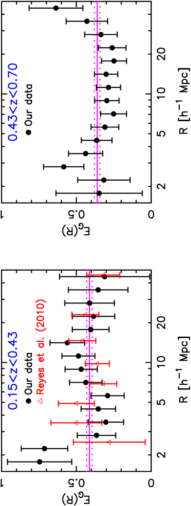
The final results are displayed in Figure 15, corresponding to a $\approx 20\%$ determination of $E_{G}$ at each scale and redshift. We overplot the GR model prediction at each redshift, $E_{G}=\Omega_{m}/f(z)$ for our fiducial model $\Omega_{m}=0.27$ (together with its 1-$\sigma$ variation give the typical error in determination of this parameter from the CMB, $\Delta\Omega_{m}=0.02$), and the measurements of Reyes et al. (2010), which correspond to the lower-redshift bin. The covariance matrix of these $E_{G}$ measurements is shown in Figure 16.

Using the covariance matrix, we fit a model of constant $E_{G}(R)$ to the data, comparing fits over the ranges $R>2R_{0}=3\,h^{-1}$ Mpc and $R>10\,h^{-1}$ Mpc. The resulting values of $\overline{E_{G}}$ for each individual source-lens dataset are listed in Table 2. The combined measurements in the two unique redshift bins $z=(0.32,0.57)$ are $(0.40\pm 0.09,0.31\pm 0.06)$ for $R>3\,h^{-1}$ Mpc and $(0.48\pm 0.10,0.30\pm 0.07)$ for $R>10\,h^{-1}$ Mpc, and hence are not significantly sensitive to the minimum scale used. The $\chi^{2}$ of the best-fitting constant $E_{G}$ model to $R>10\,h^{-1}$ Mpc is $(5.5,5.6)$ in the two redshift bins, for 6 degrees of freedom. The consistency of these measurements with the predictions of the perturbed GR model demonstrates that this model has successfully predicted both the scale-independence of the signal, and the overall amplitude.

Our measurement agrees with the fit obtained by Reyes et al. for $z=0.32$, $\overline{E_{G}}=0.39\pm 0.07$. The errors obtained in the value of $\overline{E_{G}}$ are also similar; the Reyes et al. measurements are based on SDSS imaging data which covers much wider area, but provides a significantly lower density of measured shapes.

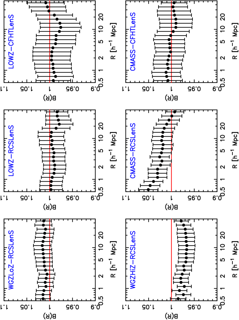
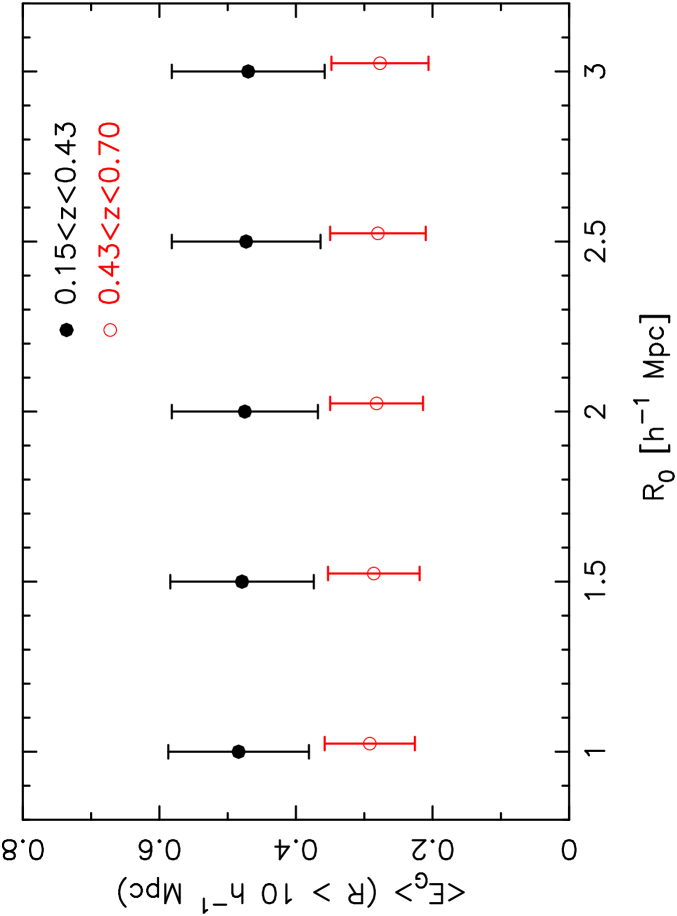
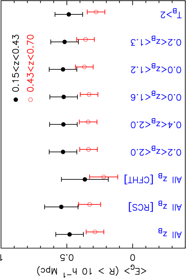
We now test the sensitivity of our measurements to two important analysis choices. First, in Figure 17 we show the results of repeating these fits of $\overline{E_{G}}$ to the range $R>10\,h^{-1}$ Mpc, in the two redshift bins, for different choices of the parameter $R_{0}$ used for small-scale suppression when measuring $\Upsilon_{gm}$ and $\Upsilon_{gg}$, in the range $1<R_{0}<3\,h^{-1}$ Mpc. These results show that our measurement of $\overline{E_{G}}$ is insensitive to the choice of $R_{0}$. Secondly, in Figure 18 we compare the fiducial measurements to repeated fits applying different cuts in the range of photometric redshifts included in the analysis: $0.2<z_{B}<2.0$, $0.4<z_{B}<2.0$, $0<z_{B}<1.6$, $0<z_{B}<1.2$ and $0.2<z_{B}<1.3$. We also show results just including RCSLenS or CFHTLenS regions, and for a “blue” sub-sample selected by a cut $T_{B}>2$ (which will be subject to a lower level of intrinsic alignments, as discussed in Section A.4). The measured values of $\overline{E_{G}}$ never differ by a significant amount from the fiducial case.

Finally, we assess the significance of any bias in the mean or standard deviation of $E_{G}$ induced by non-Gaussianity in its posterior probability distribution. Since it is a ratio of noisy quantities, the error distribution of $E_{G}$ is not necessarily Gaussian, even if the numerator and denominator are Gaussian-distributed. We compared the mean and standard deviation obtained from direct error propagation with the distributions arising from Monte-Carlo sampling the relevant quantities in the numerator and denominator. We found that, averaging over bins with $R>10\,h^{-1}$ Mpc, the mean of $E_{G}$ was biased low by $\Delta E_{G}=(0.03,0.01)$ in the two redshift ranges $z=(0.32,0.57)$, which is just under half the statistical error for the lower-redshift bin (the greater impact in the lower-redshift bin is driven by the greater fractional error in $\beta$). The width of the 1-$\sigma$ and 2-$\sigma$ confidence regions agreed within $5\%$ for the two cases. We conclude that systematic errors due to skewness in the $E_{G}$ distribution are sub-dominant to statistical errors.

An additional issue would arise if the numerator and denominator of the $E_{G}$ relation are additionally correlated, since then the mean (or median or mode) of the ratio would not be an unbiased estimator of the true value (e.g. Viola et al. 2014, Marian et al. 2015). We have estimated the correlation strength between the galaxy clustering and the galaxy-galaxy lensing correlation functions using Gaussian analytic covariances and found the correlation to be negligible. This is driven by two effects: (a) the samples studied in this work are dominated by shot noise rather than cosmic variance, which tends to de-correlate two-point statistics, and (b) $w_{p}$ and $\Delta\Sigma$ are related to the underlying matter power spectrum via different weighting functions, such that the same separations in $w_{p}$ and $\Delta\Sigma$ are sensitive to different ranges of $P_{mm}(k)$.

Figure 16: Covariance matrix of the $E_{G}(R)$ measurements in the two redshift bins, displayed as a correlation matrix $C_{ij}/\sqrt{C_{ii}C_{jj}}$.

Figure 17: The dependence of the fit of constant $\overline{E_{G}}$ to the range of scales $R>10\,h^{-1}$ Mpc on the value of $R_{0}$ chosen for the small-scale suppression in the annular differential surface density statistics.

Figure 18: The dependence of the fit of constant $\overline{E_{G}}$ to the range of scales $R>10\,h^{-1}$ Mpc on the range of photometric redshifts allowed in the analysis.

Table 2: Values of constant $E_{G}$ fit to the measurements for each combination of source-lens datasets, using the range of scales $R>3\,h^{-1}$ Mpc and $R>10\,h^{-1}$ Mpc. Best-fitting values of $\chi^{2}$ are shown for each case, and the measurements of the input RSD parameter $\beta$.

Survey	$\beta$	$\overline{E_{G}}(R>3\,h^{-1}{\rm Mpc})$	$\chi^{2}$/dof	$\overline{E_{G}}(R>10\,h^{-1}{\rm Mpc})$	$\chi^{2}$/dof
WGZLoZ-RCSLenS	$0.65\pm 0.10$	$0.36\pm 0.15$	$16.5/11$	$0.52\pm 0.21$	$13.3/6$
LOWZ-RCSLenS	$0.38\pm 0.11$	$0.40\pm 0.14$	$13.6/11$	$0.54\pm 0.15$	$4.1/6$
LOWZ-CFHTLenS	$0.38\pm 0.11$	$0.41\pm 0.16$	$8.4/11$	$0.36\pm 0.18$	$4.9/6$
WGZHiZ-RCSLenS	$0.63\pm 0.08$	$0.38\pm 0.15$	$10.0/11$	$0.27\pm 0.17$	$8.1/6$
CMASS-RCSLenS	$0.36\pm 0.06$	$0.36\pm 0.08$	$18.9/11$	$0.36\pm 0.09$	$13.3/6$
CMASS-CFHTLenS	$0.36\pm 0.06$	$0.24\pm 0.09$	$10.8/11$	$0.23\pm 0.11$	$5.9/6$
Combined $0.15<z<0.43$	-	$0.40\pm 0.09$	$10.3/11$	$0.48\pm 0.10$	$5.5/6$
Combined $0.43<z<0.70$	-	$0.31\pm 0.06$	$8.1/11$	$0.30\pm 0.07$	$5.6/6$

7 Conclusions

In this study we have performed a new test of gravitational physics based on a consistency check between the amplitude of peculiar velocities, measured via redshift-space distortion in galaxy samples from the WiggleZ and BOSS surveys, and the galaxy-galaxy lensing signal imprinted in the shapes of background galaxies in the CFHTLenS and RCSLenS datasets by density fluctuations traced by these lenses. Our results agree with the predictions of GR for a perturbed FRW metric, in a flat $\Lambda$CDM Universe with matter density consistent with observations of the CMB.

In particular we produce new measurements of the “gravitational slip” statistic $E_{G}=\Upsilon_{gm}/(\beta\,\Upsilon_{gg})$, estimating values $0.48\pm 0.10$ at $z=0.32$ and $0.30\pm 0.07$ at $z=0.57$ when averaging over scales $10<R<50\,h^{-1}$ Mpc, compared to model predictions of $E_{G}=0.41$ and $0.36$, respectively. The results are consistent with those obtained when averaging over $3<R<50\,h^{-1}$ Mpc. When carrying out this measurement we suppressed small-scale information from $R<R_{0}=1.5\,h^{-1}$ Mpc using the annular differential surface density statistic, although we find that our results are in fact insensitive to the choice of $R_{0}$.

Assuming a $\Lambda$CDM cosmological model and fixing all the parameters apart from $\sigma_{8}$, we determine $\sigma_{8}(z=0.32)=0.75\pm 0.08$ and $\sigma_{8}(z=0.57)=0.54\pm 0.07$ by fitting to the differential surface density $\Delta\Sigma$ and projected lens correlation function $w_{p}$, after marginalizing over separate linear bias factors of each lens sample. These results are also consistent with the expected growth of structure in a perturbed $\Lambda$CDM Universe.

In terms of methodology, we particularly note the systematic bias that can occur in the measurement of $\Delta\Sigma(R)$ when using photo-$z$ information to select source-lens pairs, and how this can be reduced by using the full redshift probability of each source in the estimator. We find that our results are not sensitive to the range of photometric redshifts included in the analysis.

We note that a measurement of $E_{G}$ using lensing of the Cosmic Microwave Background by BOSS-CMASS galaxies was recently presented by Pullen et al. (2015), determining $E_{G}(z=0.57)=0.243\pm 0.060{\rm(stat)}\pm 0.013{\rm(sys)}$. This measurement is consistent with ours, with both results lying below the standard model prediction.

Combinations of gravitational lensing and redshift-space distortion data offer a powerful opportunity to test large-scale gravitational physics in the search for an understanding of the physical nature of dark energy. Datasets such as CFHTLenS, RCSLenS, the Kilo-Degree Survey (KiDS), Dark Energy Survey (DES) and the Hyper-Suprime Cam (HSC) lensing survey, promise that the constraining power of such tests will continue to improve rapidly and provide increasingly stringent tests of fundamental cosmology.

Appendix A Calibration corrections and systematics tests

A.1 Systematics tests manipulating source shears

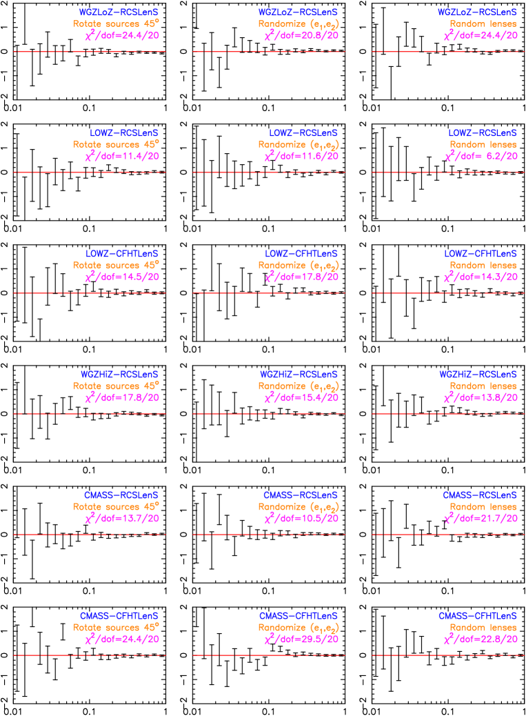
We performed a series of systematics tests manipulating the source and lens catalogues and re-measuring the average tangential shear $\gamma_{t}(\theta)$:

• We rotated the sources by $45^{\circ}$ (i.e., $e_{1,{\rm new}}=e_{2,{\rm old}}$ and $e_{2,{\rm new}}=-e_{1,{\rm old}}$).

• We randomized the shears (i.e., randomly shifted each pair of values $(e_{1},e_{2})$ to a different source galaxy).

• We replaced the lens catalogue by a random catalogue.

The results of these tests are shown in Figure 19; in all cases we should find $\gamma_{t}(\theta)=0$ in the absence of systematic errors. The covariance matrices for each measurement are obtained by applying the same systematics-test operation to each mock catalogue; this covariance allows us to evaluate the $\chi^{2}$ statistic of the $\gamma_{t}=0$ model in each case. These values are printed in each panel along with the number of degrees of freedom, ${\rm dof}=20$, and indicate consistency with the model.

Figure 19: Systematics tests of the $\gamma_{t}(\theta)$ measurement applied to the galaxy-galaxy lensing cross-correlations for the different combinations of source-lens datasets. The $x$-axis is the angular separation $\theta$ in degrees, the $y$-axis plots $10^{5}\gamma_{t}$. The left, middle, and right columns respectively show measurements following rotation of sources by $45^{\circ}$, randomization of shear values, and replacement of the lens catalogue by a random catalogue. $\chi^{2}$ statistics are quoted for the measurements with respect to a model of zero, indicated by the horizontal line.

A.2 Shear bias calibration corrections

The effect of the additive shear calibration bias is negligible for galaxy-galaxy lensing. Figure 20 displays the multiplicative shear bias corrections $K(\theta)$ and $K(R)$, defined by Equations 33 and 35, which are applied to the galaxy-galaxy lensing measurements by multiplying the estimated values by $(1+K)^{-1}$. Corrections are shown for each combination of source-lens datasets, combining the different survey fields. These corrections are approximately independent of scale and have values $K\approx-0.06$. We note that the determinations of $K(R)$ depend on the redshift distribution of the source and lens samples, through the weighting factor $\Sigma_{c}^{-1}$, which imprints an extra variation between datasets compared to $K(\theta)$.

A.3 Photo-$z$ systematic test: SIS fits in $z_{B}$ slices

Systematic errors in the BPZ photometric redshift probability distributions would imprint errors in the determination of $\Delta\Sigma(R)$, which relies on the computation of $\overline{\Sigma_{c}^{-1}}$ for each source-lens pair from an integral over redshift weighted by $p_{\rm BPZ}(z)$, and in the cosmological modelling, which uses the source redshift probability distribution $p_{s}(z)$ derived from stacking the individual $p_{\rm BPZ}(z)$ functions. We tested for such systematics by computing the amplitude of the tangential shear around a fixed set of foreground lenses in a series of eight photometric redshift bins defined using $z_{B}$ – $(0-0.2,0.2-0.4,0.4-0.6,0.6-0.8,0.8-1.0,1.0-1.2,1.2-1.6)$ – in order to determine whether this amplitude scaled with redshift in the expected manner. A convenient method for quantifying the results is to assume a singular isothermal sphere (SIS) model for the lenses, characterized by a velocity dispersion $\sigma_{v}$, and to verify that the values of $\sigma_{v}$ derived from the shear of each photo-$z$ source slice are consistent. The shear profile for SIS lenses is given in terms of the Einstein radius $\theta_{E}$ by $\gamma_{t}(\theta)=\theta_{E}/2\theta$, where

$$\theta_{E}=4\pi\left(\frac{\sigma_{v}}{c}\right)^{2}\left<\frac{D_{ls}}{D_{s}}\right>,$$ (40)

and the geometrical factor is given by

$$\left<\frac{D_{ls}}{D_{s}}\right>=\int_{0}^{\infty}dz\,p_{l}(z)\int_{z}^{\infty}dz^{\prime}\,p_{s}(z^{\prime})\left[\frac{\chi(z^{\prime})-\chi(z)}{\chi(z^{\prime})}\right].$$ (41)

Figure 21 displays the stacked RCSLenS BPZ redshift probability distributions $p_{s}(z)$, weighted by the lensfit weights, in each of the photo-$z$ slices. A signal is produced even for low values of $z_{B}$, because sources are scattered to apparent low redshifts from true higher redshifts.

Figure 22 displays the fits for the $\sigma_{v}$ parameter of the four different lens samples – WGZLoZ, WGZHiZ, LOWZ and CMASS – in each photo-$z$ bin, using these $p(z_{s})$ functions determined from the outputs of BPZ. The fits are performed to $\gamma_{t}(\theta)$ measurements in the range $0.01^{\circ}<\theta<1^{\circ}$. The inferred values of $\sigma_{v}$ are generally consistent as the source photo-$z$ slice changes, with the possible exception of the lowest redshift slice $0<z_{B}<0.2$ for CFHTLenS, which contains a negligible number of galaxies.

A.4 Intrinsic alignments systematic test: SIS fits to $T_{B}$ samples

Another potential systematic effect that could impact our measurements is the intrinsic alignment of the background source sample with the foreground lens distribution. This effect is expected to preferentially diminish the average tangential shear of red source galaxies compared to blue galaxies. The BPZ pipeline returns a source galaxy type in the range $0\leq T_{B}\leq 6$, and we used this parameter to divide the sources into sub-samples of red ($T_{B}<2$) and blue ($T_{B}>2$) galaxies. Following Section A.3, we then determined the velocity dispersion of foreground lenses in the SIS model for the blue, red and combined source samples in the range $0.2<z_{B}<1.6$. We also performed measurements for a blue sample over a photo-$z$ range significantly higher than the maximum redshift of the spectroscopic lenses ($0.9<z_{B}<1.6$ for WGZHiZ and CMASS, and $0.6<z_{B}<1.6$ for WGZLoZ and LOWZ. The source distributions $p_{s}(z)$ for each case were determined by stacking the appropriate subset of BPZ redshift distributions. Results are displayed in Figure 23. The inferred values of $\sigma_{v}$ are again generally consistent amongst the samples, with the possible exception of the cross-correlations between CFHTLenS and BOSS red galaxies. However, as shown in Figure 18, the fitted value of $E_{G}$ is not significantly affected by cutting the sources to a blue sample.

Figure 20: Multiplicative shear bias corrections to be applied to $\gamma_{t}(\theta)$ (upper panel) and $\Delta\Sigma(R)$ (lower panel), for the different combinations of source-lens datasets.

Figure 21: Stacked RCSLenS BPZ redshift probability distributions, weighted by the lensfit weights, in a series of $z_{B}$ slices.

Figure 22: The SIS velocity dispersion fit to the average tangential shear around a series of foreground lens samples, for different sets of sources in photometric redshift slices split by $z_{B}$. The source redshift distributions for each slice, needed to model the resulting signal, are obtained from the stacked BPZ redshift probability distributions obtained for each source.

Figure 23: The SIS velocity dispersion fit to the average tangential shear around a series of foreground lens samples, for different sets of sources split by galaxy type according to $T_{B}$. The source redshift distributions for each slice, needed to model the resulting signal, are obtained from the stacked BPZ redshift probability distributions obtained for each source.

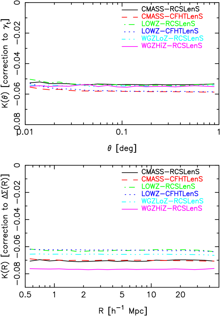
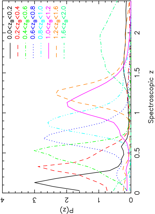
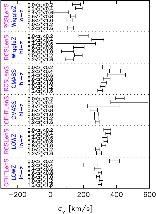
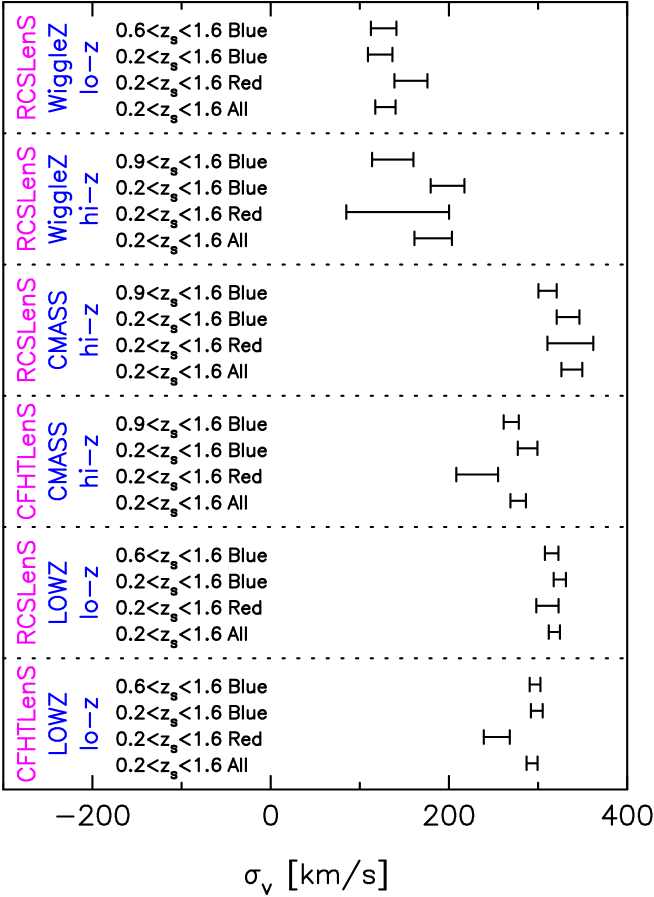
A.5 Source-lens association correction $B(R)$

Some sources may be clustered or associated with the lenses, but scattered to higher redshifts by photo-$z$ errors. These sources will not be lensed, diluting the cross-correlation signal. The strength of this effect may be determined by measuring the excess in the number counts of source galaxies in the vicinity of lens galaxies, compared to a random distribution of lenses. The resulting multiplicative bias in the measurement of $\Delta\Sigma(R)$ may be corrected by boosting the signal by

$$B(R)=\frac{\sum_{{\rm sources}\,i}\sum_{{\rm data\,lenses}\,j}w^{s}_{i}\,w^{l}_{j}\,\Sigma_{c,ij}^{-1}\,\Theta(i,j)}{\sum_{{\rm sources}\,i}\sum_{{\rm random\,lenses}\,j}w^{s}_{i}\,w^{r}_{j}\,\Sigma_{c,ij}^{-1}\,\Theta(i,j)},$$ (42)

where $w^{r}$ denotes the weights of the random lenses (normalized such that $\sum_{j}w^{r}_{j}=\sum_{j}w^{l}_{j}$), and where $\Sigma_{c,ij}^{-1}$ should be replaced by $\overline{\Sigma_{c}^{-1}}_{ij}$ when moving from the estimator of Equation 30 to 28.

Figure 24 displays the boost factors $B(R)$ for shapes in the different RCSLenS and CFHTLenS regions correlated with WiggleZ and BOSS lenses, averaging over 40 random catalogues. The signal is generally consistent with $B=1$, with deviations at the level of $3\%$ or below for scales $R>2\,h^{-1}$ Mpc. We do not apply this correction to our measurements.

We note that an effect $B(R)<1$, which is not expected through physical association, may be obtained if there is an anti-correlation between sources and lenses (for example, star-forming galaxies avoid dense environments on small scales), or through instrumental effects impacting the imaging data (such as contamination from light of foreground galaxies or sky subtraction).

Figure 24: Boost factor $B(R)$ from source-lens clustering for the different combinations of source and lens samples analyzed in this study. The measurements are the average over 40 random catalogues, with the errors indicating the standard deviation between the catalogues.

References

- [1] Anderson, L., et al, 2014, MNRAS, 441, 24
- [2] Aubourg, E., et al., 2015, submitted (arXiv:1411.1074)
- [3] Baldauf, T., Smith, R.E., Seljak, U., Mandelbaum, R., 2010, PhRvD, 81 3531
- [4] Bartelmann, M., Schneider, P., 2001, PhR, 340, 291
- [5] Benitez, N., 2000, ApJ, 536, 571
- [6] Betoule, M., et al., 2014, A&A, 568, 22
- [7] Beutler, F., et al., 2012, MNRAS, 423, 3430
- [8] Blake, C.A., et al., 2009, MNRAS, 395, 240
- [9] Blake, C.A., et al., 2010, MNRAS, 406, 803
- [10] Blake, C.A., et al., 2011, MNRAS, 415, 2892
- [11] Blazek, J., Mandelbaum, R., Seljak, U., Nakajima, R., 2012, JCAP, 5, 41
- [12] Cacciato, M., van den Bosch, F.C., More, S., Mo, H., Yang, X., 2013, MNRAS, 430, 767
- [13] Cacciato, M., van Uitert, E., Hoekstra, H., 2014, MNRAS, 437, 377
- [14] Chang, C., et al., 2013, MNRAS, 434, 2121
- [15] Chuang, C.-H., et al., 2014, submitted (arXiv:1312.4889)
- [16] Dawson, K.S, et al., 2013, AJ, 145, 10
- [17] de la Torre, S., et al., 2013, A&A, 557, 54
- [18] Drinkwater, M.J., et al., 2010, MNRAS, 401, 1429
- [19] Eisenstein, D.J., et al., 2011, AJ, 142, 72
- [20] Erben, T., et al., 2013, MNRAS, 433, 2545
- [21] Gilbank, D.G., Gladders, M.D., Yee, H.K.C., Hsieh, B.C., 2011, AJ, 141, 94
- [22] Guzik, J., Seljak, U., 2001, MNRAS, 321, 439
- [23] Harnois-Deraps, J., Vafaei, S., van Waerbeke, L., 2012, MNRAS, 426, 1262
- [24] Harnois-Deraps, J., van Waerbeke, L., 2015, MNRAS, 450, 2857
- [25] Hartlap, J., Simon, P., Schneider, P., 2007, A&A, 464, 399
- [26] Heymans, C., et al., 2012, MNRAS, 427, 146
- [27] Heymans, C., et al., 2013, MNRAS, 432, 2433
- [28] Hildebrandt, H., et al., 2012, MNRAS, 421, 2355
- [29] Hildebrandt, H., et al., 2015, in preparation
- [30] Hu, W., Jain, B., 2004, PhRvD, 70, 3009
- [31] Jain, B., Zhang, P., 2008, PhRvD, 78, 3503
- [32] Joachimi, B., Bridle, S.L, 2010, A&A, 523, 1
- [33] Kaiser, N., 1987, MNRAS, 227, 1
- [34] Komatsu, E., et al., 2011, ApJS, 192, 18
- [35] Kuijken, K., et al., 2015, MNRAS, 454, 3500
- [36] Leonard, C.D., Ferreira, P.G., Heymans, C., Miller, L., 2015, in preparation
- [37] Lewis, A., Challinor, A., Lasenby, A., 2000, ApJ, 538, 473
- [38] Mandelbaum, R., et al., 2005, MNRAS, 361, 1287
- [39] Mandelbaum, R., Seljak, U., Baldauf, T., Smith, R.E., 2010, MNRAS, 405, 2078
- [40] Mandelbaum, R., Slosar, A., Baldauf, T., Seljak, U., Hirata, C.M., Nakajima, R., Reyes, R., Smith, R.E., 2013, MNRAS, 432, 1544
- [41] Marian, L., Smith, R.E., Angulo, R.E., 2015, MNRAS, 451, 1418
- [42] Miller, L., et al., 2013, MNRAS, 429, 2858
- [43] Miyatake, H., et al., 2015, ApJ, 806, 1
- [44] More, S., Miyatake, H., Mandelbaum, R., Takada, M., Spergel, D., Brownstein, J., Schneider, D.P., 2015, ApJ, 806, 2
- [45] Nakajima, R., Mandelbaum, R., Seljak, U., Cohn, J., Reyes, R., Cool, R., 2012, MNRAS, 420, 3240
- [46] Percival, W.J., White, M., 2009, MNRAS, 393, 297
- [47] Planck collaboration, 2015a, submitted (arXiv:1502.01590)
- [48] Planck collaboration, 2015b, submitted (arXiv:1502.01589)
- [49] Pullen, A.R., Alam, S., He, S., Ho., S., 2015, MNRAS, submitted (arXiv:1511.04457)
- [50] Reid, B., et al., 2012, MNRAS, 426, 2719
- [51] Reyes, R., Mandelbaum, R., Seljak, U., Baldauf, T., Gunn, J.E., Lombriser, L., Smith, R.E., 2010, Nature, 464, 256
- [52] Samushia, L., et al., 2014, MNRAS, 439, 3504
- [53] Sanchez, A.G., et al., 2014, MNRAS, 440, 2692
- [54] Scherrer, R.J., Weinberg, D.H., 1998, ApJ, 504, 607
- [55] Seitz, C., Schneider, P., 1997, A&A, 318, 687
- [56] Simpson, F., et al., 2013, MNRAS, 429, 2249
- [57] Smith, R.E., et al., 2003, MNRAS, 341, 1311
- [58] van Uitert, E., Hoekstra, H., Velander, M., Gilbank, D.G., Gladders, M.D., Yee, H.K.C., 2011, A&A, 534, 14
- [59] van Uitert, E., Hoekstra, H., Schrabback, T., Gilbank, D.G., Gladders, M.D., Yee, H.K.C., 2012, A&A, 545, 71
- [60] van Uitert, E., Hoekstra, H., Franx, M., Gilbank, D.G., Gladders, M.D., Yee, H.K.C., 2013, A&A, 549, 7
- [61] van Uitert, E., Cacciato, M., Hoekstra, H., Herbonnet, R., 2015, A&A, 579, 26
- [62] Velander, M., et al., 2014, MNRAS, 437, 2111
- [63] Zhang, P., Liguori, M., Bean, R., Dodelson, S., 2007, PhRvL, 99, 1302