Estimation of Laplacian spectra of direct and strong product graphs

Abstract

Calculating a product of multiple graphs has been studied in mathematics, engineering, computer science, and more recently in network science, particularly in the context of multilayer networks. One of the important questions to be addressed in this area is how to characterize spectral properties of a product graph using those of its factor graphs. While several such characterizations have already been obtained analytically (mostly for adjacency spectra), characterization of Laplacian spectra of direct product and strong product graphs has remained an open problem. Here we develop practical methods to estimate Laplacian spectra of direct and strong product graphs from spectral properties of their factor graphs using a few heuristic assumptions. Numerical experiments showed that the proposed methods produced reasonable estimation with percentage errors confined within a $\pm 10$% range for most eigenvalues.

1 Introduction

Calculating a product of multiple graphs has been studied in several disciplines. In mathematics, multiplication of graphs has been studied with a particular interest in their algebraic properties as matrix operators and their implications for topologies of resulting graphs [13, 14, 4, 6, 5]. Graph products also appear in engineering as an efficient way to describe discretized structure of objects in structural mechanics [8, 7], and in computer science as a generative model of complex networks [12, 11, 10]. More recently, graph products have also began to appear in network science, particularly in the context of multilayer networks, where multiplication of graphs are often used as a formal way to describe certain types of multilayer network topologies [3, 17, 9, 15, 16]. One of the important questions to be addressed in this area is how to characterize spectral properties of a product graph using those of its factor graphs, especially those of Laplacian matrices because of their high relevance to network structure and dynamics.

Several such spectral characterizations have already been obtained analytically for certain product graphs, but they are mostly for adjacency spectra. Characterization of Laplacian spectra has so far been done only for Cartesian product graphs. In the meantime, there are other important forms of graph products, such as direct product and strong product [5], but characterization of Laplacian spectra of those product graphs has turned out to be quite challenging and has remained an open problem to date.

In this paper, we attempt to address this problem by developing practical, computationally efficient methods to estimate Laplacian spectra of direct and strong product graphs from spectral properties of their factor graphs, using a few heuristic assumptions. We evaluated the effectiveness of our proposed methods through numerical experiments, which demonstrated that they successfully produced reasonable estimation of Laplacian spectra with percentage errors confined within a $\pm 10$% range for most eigenvalues.

The rest of the paper is structured as follows: In Section 2 we define three fundamental forms of graph products and describe how they can be represented as operations of adjacency matrices. In Section 3 we summarize spectral properties of product graphs that are already known. In Section 4 we design our new methods to estimate Laplacian spectra of direct and strong product graphs, and then evaluate their effectiveness by numerical experiments. Finally, we conclude this paper with discussions of the limitation of the current work and directions of future research in Section 5.

2 Product graphs

Let $G=(V_{G},E_{G})$ and $H=(V_{H},E_{H})$ be two simple connected graphs, where $V_{G}$ (or $V_{H}$) and $E_{G}$ (or $E_{H}$) are the sets of nodes and edges of $G$ (or $H$), respectively. We denote an adjacency matrix of graph $X$ as $A_{X}$. We also use $I_{n}$ to represent an $n\times n$ identity matrix.

We consider operations that create a product graph of $G$ and $H$. We call $G$ and $H$ factor graphs of the product. The node set of a product graph will be a Cartesian product of $V_{G}$ and $V_{H}$ (i.e., $\{(g,h)\;|\;g\in V_{G},\,h\in V_{H}\}$). Several graph product operators have been proposed and studied in mathematics, which differ from each other regarding how to connect those nodes in the product graph. In this paper, we focus on the following three fundamental graph products [5]:

$G:$		$\displaystyle A_{G}=\begin{pmatrix}0&1&0&0\\ 1&0&1&1\\ 0&1&0&0\\ 0&1&0&0\end{pmatrix}$
$H:$		$\displaystyle A_{H}=\begin{pmatrix}0&1&1\\ 1&0&1\\ 1&1&0\end{pmatrix}$

(a) Cartesian product $G\Box H$
	$\begin{array}[]{rl}A_{G\Box H}&=A_{G}\oplus A_{H}\\ &=A_{G}\otimes I_{|V_{H}|}+I_{|V_{G}|}\otimes A_{H}\\ &={\footnotesize\left(\begin{array}[]{ccc|ccc|ccc|ccc}0&1&1&1&0&0&0&0&0&0&0&0\\ 1&0&1&0&1&0&0&0&0&0&0&0\\ 1&1&0&0&0&1&0&0&0&0&0&0\\ \hline\cr 1&0&0&0&1&1&1&0&0&1&0&0\\ 0&1&0&1&0&1&0&1&0&0&1&0\\ 0&0&1&1&1&0&0&0&1&0&0&1\\ \hline\cr 0&0&0&1&0&0&0&1&1&0&0&0\\ 0&0&0&0&1&0&1&0&1&0&0&0\\ 0&0&0&0&0&1&1&1&0&0&0&0\\ \hline\cr 0&0&0&1&0&0&0&0&0&0&1&1\\ 0&0&0&0&1&0&0&0&0&1&0&1\\ 0&0&0&0&0&1&0&0&0&1&1&0\end{array}\right)}\end{array}$
(b) Direct (tensor) product $G\times H$
	$\begin{array}[]{rl}A_{G\times H}&=A_{G}\otimes A_{H}\\ &={\footnotesize\left(\begin{array}[]{ccc|ccc|ccc|ccc}0&0&0&0&1&1&0&0&0&0&0&0\\ 0&0&0&1&0&1&0&0&0&0&0&0\\ 0&0&0&1&1&0&0&0&0&0&0&0\\ \hline\cr 0&1&1&0&0&0&0&1&1&0&1&1\\ 1&0&1&0&0&0&1&0&1&1&0&1\\ 1&1&0&0&0&0&1&1&0&1&1&0\\ \hline\cr 0&0&0&0&1&1&0&0&0&0&0&0\\ 0&0&0&1&0&1&0&0&0&0&0&0\\ 0&0&0&1&1&0&0&0&0&0&0&0\\ \hline\cr 0&0&0&0&1&1&0&0&0&0&0&0\\ 0&0&0&1&0&1&0&0&0&0&0&0\\ 0&0&0&1&1&0&0&0&0&0&0&0\end{array}\right)}\end{array}$
(c) Strong product $G\boxtimes H$
	$\begin{array}[]{rl}A_{G\boxtimes H}&=A_{G}\oplus A_{H}+A_{G}\otimes A_{H}\\ &=(A_{G}+I_{|V_{G}|})\otimes(A_{H}+I_{|V_{H}|})-I_{|V_{G}|}\otimes I_{|V_{H}|}\\ &={\footnotesize\left(\begin{array}[]{ccc|ccc|ccc|ccc}0&1&1&1&1&1&0&0&0&0&0&0\\ 1&0&1&1&1&1&0&0&0&0&0&0\\ 1&1&0&1&1&1&0&0&0&0&0&0\\ \hline\cr 1&1&1&0&1&1&1&1&1&1&1&1\\ 1&1&1&1&0&1&1&1&1&1&1&1\\ 1&1&1&1&1&0&1&1&1&1&1&1\\ \hline\cr 0&0&0&1&1&1&0&1&1&0&0&0\\ 0&0&0&1&1&1&1&0&1&0&0&0\\ 0&0&0&1&1&1&1&1&0&0&0&0\\ \hline\cr 0&0&0&1&1&1&0&0&0&0&1&1\\ 0&0&0&1&1&1&0&0&0&1&0&1\\ 0&0&0&1&1&1&0&0&0&1&1&0\end{array}\right)}\end{array}$

Figure 1: Three fundamental graph products. Top: Two factor graphs used in this example, $G$ and $H$, and their adjacency matrices. (a) Cartesian product. (b) Direct (tensor) product. (c) Strong product. Solid and dashed lines are intra-layer and inter-layer edges, respectively. Here, $G$ is considered an inter-layer network that connects the intra-layer network $H$, but one can consider the other way around too.

Cartesian product:

Denoted as $G\Box H$. Two nodes $(g,h)$ and $(g^{\prime},h^{\prime})$ are connected in $G\Box H$ if and only if

$$g=g^{\prime}\text{~{}~{}and~{}~{}}(h,h^{\prime})\in E_{H},\quad\text{or}\quad(g,g^{\prime})\in E_{G}\text{~{}~{}and~{}~{}}h=h^{\prime}.$$ (1)

The adjacency matrix of $G\Box H$ is given by

$$A_{G\Box H} =A_{G}\oplus A_{H}$$ (2)

$$=A_{G}\otimes I_{|V_{H}|}+I_{|V_{G}|}\otimes A_{H},$$ (3)

where $\oplus$ and $\otimes$ denote a Kronecker sum and a Kronecker product of matrices, respectively. An example is shown in Fig. 1(a).

Direct (tensor) product:

Denoted as $G\times H$. Two nodes $(g,h)$ and $(g^{\prime},h^{\prime})$ are connected in $G\times H$ if and only if

$$(g,g^{\prime})\in E_{G}\text{~{}~{}and~{}~{}}(h,h^{\prime})\in E_{H}.$$ (4)

The adjacency matrix of $G\times H$ is given by

$$A_{G\times H} =A_{G}\otimes A_{H}.$$ (5)

An example is shown in Fig. 1(b).

Strong product:

Denoted as $G\boxtimes H$. Two nodes $(g,h)$ and $(g^{\prime},h^{\prime})$ are connected in $G\boxtimes H$ if and only if

$$g=g^{\prime}\text{~{}~{}and~{}~{}}(h,h^{\prime})\in E_{H},\quad\text{or}\quad(g,g^{\prime})\in E_{G}\text{~{}~{}and~{}~{}}h=h^{\prime},\quad\text{or}\quad(g,g^{\prime})\in E_{G}\text{~{}~{}and~{}~{}}(h,h^{\prime})\in E_{H}.$$ (6)

The adjacency matrix of $G\boxtimes H$ is given by

$$A_{G\boxtimes H} =A_{G}\oplus A_{H}+A_{G}\otimes A_{H}$$ (7)

$$=(A_{G}+I_{|V_{G}|})\otimes(A_{H}+I_{|V_{H}|})-I_{|V_{G}|}\otimes I_{|V_{H}|}.$$ (8)

As seen above, a strong product is a sum of Cartesian and direct products. An example is shown in Fig. 1(c).

All of these three graph products are commutative, in the sense that $G*H$ and $H*G$ (where $*$ can be either $\Box$, $\times$, or $\boxtimes$) are isomorphic to each other. These operations are also associative.

3 Spectral properties of product graphs

Relationships between spectral properties of a product graph and those of its factor graphs have been known for degree and adjacency spectra for all of the three products, as well as Laplacian spectra for Cartesian product [13, 4, 7, 1]. They are summarized below.

3.1 Degree spectra

Let $\mathbbm{1}_{n}$ be an all-one column vector with length $n$. Then the degree spectrum (i.e., degree sequence) of graph $X$ can be obtained as $d^{X}=A_{X}\mathbbm{1}_{|V_{X}|}$. Here we denote the degree spectra of graphs $G$ and $H$ as $d^{G}=\big{(}d^{G}_{i}\big{)}$ and $d^{H}=\big{(}d^{H}_{j}\big{)}$, respectively ($i=1,2,\ldots,|V_{G}|,\;j=1,2,\ldots,|V_{H}|$). Applying this to the adjacency matrices of product graphs yields the following (note that $\mathbbm{1}_{|V_{G}|\cdot|V_{H}|}=\mathbbm{1}_{|V_{G}|}\otimes\mathbbm{1}_{|V_{H}|}$):

Cartesian product:

$$A_{G\Box H}\mathbbm{1}_{|V_{G}|\cdot|V_{H}|} =(A_{G}\otimes I_{|V_{H}|})(\mathbbm{1}_{|V_{G}|}\otimes\mathbbm{1}_{|V_{H}|})+(I_{|V_{G}|}\otimes A_{H})(\mathbbm{1}_{|V_{G}|}\otimes\mathbbm{1}_{|V_{H}|})$$ (9)

$$=d^{G}\otimes\mathbbm{1}_{|V_{H}|}+\mathbbm{1}_{|V_{G}|}\otimes d^{H}$$ (10)

$$=\bigg{(}d^{G}_{i}+d^{H}_{j}\bigg{)}$$ (11)

Direct product:

$$A_{G\times H}\mathbbm{1}_{|V_{G}|\cdot|V_{H}|} =(A_{G}\otimes A_{H})(\mathbbm{1}_{|V_{G}|}\otimes\mathbbm{1}_{|V_{H}|})$$ (12)

$$=d^{G}\otimes d^{H}$$ (13)

$$=\bigg{(}d^{G}_{i}\,d^{H}_{j}\bigg{)}$$ (14)

Strong product:

$$A_{G\boxtimes H}\mathbbm{1}_{|V_{G}|\cdot|V_{H}|} =A_{G\Box H}\mathbbm{1}_{|V_{G}|\cdot|V_{H}|}+A_{G\times H}\mathbbm{1}_{|V_{G}|\cdot|V_{H}|}$$ (15)

$$=\bigg{(}d^{G}_{i}+d^{H}_{j}+d^{G}_{i}\,d^{H}_{j}\bigg{)}$$ (16)

3.2 Adjacency spectra

Adjacency spectra (i.e., eigenvalues of adjacency matrices) of product graphs can be obtained in a similar manner. Let $\{\lambda^{G}_{i}\}$ and $\{\lambda^{H}_{j}\}$ be the eigenvalues of $A_{G}$ and $A_{H}$ with corresponding eigenvectors $\{v^{G}_{i}\}$ and $\{v^{H}_{j}\}$, respectively ($i=1,2,\ldots,|V_{G}|,\;j=1,2,\ldots,|V_{H}|$). Then it can be shown that for all of the three product graphs, their adjacency matrices have $v^{G}_{i}\otimes v^{H}_{j}$ as eigenvectors, as follows:

Cartesian product:

$$A_{G\Box H}(v^{G}_{i}\otimes v^{H}_{j}) =(A_{G}\otimes I_{|V_{H}|})(v^{G}_{i}\otimes v^{H}_{j})+(I_{|V_{G}|}\otimes A_{H})(v^{G}_{i}\otimes v^{H}_{j})$$ (17)

$$=\lambda^{G}_{i}v^{G}_{i}\otimes v^{H}_{j}+v^{G}_{i}\otimes\lambda^{H}_{j}v^{H}_{j}$$ (18)

$$=\bigg{(}\lambda^{G}_{i}+\lambda^{H}_{j}\bigg{)}(v^{G}_{i}\otimes v^{H}_{j})$$ (19)

Direct product:

$$A_{G\times H}(v^{G}_{i}\otimes v^{H}_{j}) =(A_{G}\otimes A_{H})(v^{G}_{i}\otimes v^{H}_{j})$$ (20)

$$=\lambda^{G}_{i}v^{G}_{i}\otimes\lambda^{H}_{j}v^{H}_{j}$$ (21)

$$=\bigg{(}\lambda^{G}_{i}\,\lambda^{H}_{j}\bigg{)}(v^{G}_{i}\otimes v^{H}_{j})$$ (22)

Strong product:

$$A_{G\boxtimes H}(v^{G}_{i}\otimes v^{H}_{j}) =A_{G\Box H}(v^{G}_{i}\otimes v^{H}_{j})+A_{G\times H}(v^{G}_{i}\otimes v^{H}_{j})$$ (23)

$$=\bigg{(}\lambda^{G}_{i}+\lambda^{H}_{j}+\lambda^{G}_{i}\,\lambda^{H}_{j}\bigg{)}(v^{G}_{i}\otimes v^{H}_{j})$$ (24)

Note the similarity of results between degree and adjacency spectra.

3.3 Laplacian spectra for Cartesian product graphs

Laplacian spectra of product graphs turn out to be not as simply characterizable as the other two shown above. So far, only a Laplacian spectrum of a Cartesian product graph has been analytically linked to Laplacian spectra of its factor graphs. Here we denote the Laplacian and degree matrices of graph $X$ as $L_{X}$ and $D_{X}$, respectively. Then the Laplacian matrix of Cartesian product graph $G\Box H$ can be characterized as follows:

$$L_{G\Box H} =D_{G\Box H}-A_{G\Box H}$$ (25)

$$=(D_{G}\otimes I_{|V_{H}}+I_{|V_{G}|}\otimes D_{H})-(A_{G}\otimes I_{|V_{H}|}+I_{|V_{G}|}\otimes A_{H})$$ (26)

$$=D_{G}\otimes I_{|V_{H}}+I_{|V_{G}|}\otimes D_{H}-(D_{G}-L_{G})\otimes I_{|V_{H}|}-I_{|V_{G}|}\otimes(D_{H}-L_{H})$$ (27)

$$=L_{G}\otimes I_{|V_{H}|}+I_{|V_{G}|}\otimes L_{H}$$ (28)

The result above shows that the relationship between Laplacians of factor and product graphs are identical to the relationship between their adjacency matrices (Eq. (3)). Therefore, the same conclusion about their spectral relationship naturally follows. Let $\{\mu^{G}_{i}\}$ and $\{\mu^{H}_{j}\}$ be the eigenvalues of $L_{G}$ and $L_{H}$ with corresponding eigenvectors $\{w^{G}_{i}\}$ and $\{w^{H}_{j}\}$, respectively ($i=1,2,\ldots,|V_{G}|,\;j=1,2,\ldots,|V_{H}|$). Then the following can be shown directly from Eq. (19):

$$L_{G\Box H}(w^{G}_{i}\otimes w^{H}_{j}) =\bigg{(}\mu^{G}_{i}+\mu^{H}_{j}\bigg{)}(w^{G}_{i}\otimes w^{H}_{j})$$ (29)

4 Laplacian spectra of direct and strong product graphs

Characterizing Laplacian spectra of direct product and strong product graphs is quite challenging and has remained an open problem. The objective of the present study is to develop practical methods to estimate their Laplacian spectra using a few heuristic assumptions, in view of potential applications for large-scale multilayer network analysis [15, 9, 2].

4.1 Estimating Laplacian spectra of direct product graphs

A Laplacian of direct product graph $G\times H$ is given as follows:

$$L_{G\times H} =D_{G\times H}-A_{G\times H}$$ (30)

$$=(D_{G}\otimes D_{H})-(A_{G}\otimes A_{H})$$ (31)

$$=D_{G}\otimes D_{H}-(D_{G}-L_{G})\otimes(D_{H}-L_{H})$$ (32)

$$=L_{G}\otimes D_{H}+D_{G}\otimes L_{H}-L_{G}\otimes L_{H}$$ (33)

A general solution for obtaining eigenvalues and eigenvectors of this Laplacian matrix from those of its factor graphs is not known to date. The complexity of the problem partly comes from the involvement of $D_{G}$ and $D_{H}$ in the formula above, which were successfully eliminated in all of the previous cases. (We will come back to this point later.) In the meantime, however, there are partial regularities known for Laplacian spectra of direct product graphs that resemble those of Cartesian product graphs, especially when either factor graph is regular [1]. Moreover, there is empirical evidence that $w^{G}_{i}\otimes w^{H}_{j}$, i.e., eigenvectors of $L_{G\Box H}$, are relatively close to eigenvectors of $L_{G\times H}$, i.e.,

$$L_{G\times H}(w^{G}_{i}\otimes w^{H}_{j})\approx\alpha(w^{G}_{i}\otimes w^{H}_{j}),$$ (34)

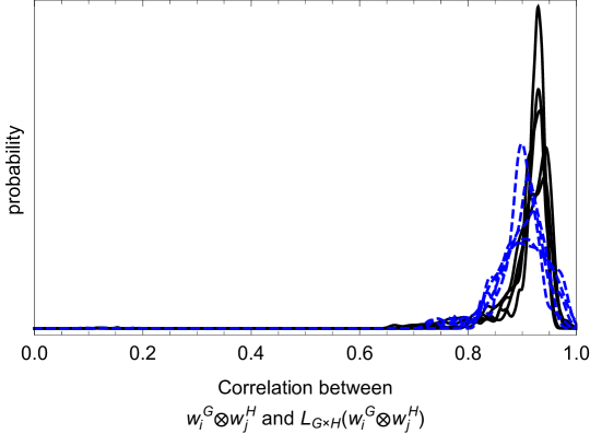
which can be numerically observed by measuring vector correlations between $w^{G}_{i}\otimes w^{H}_{j}$ and $L_{G\times H}(w^{G}_{i}\otimes w^{H}_{j})$ (Fig. 2). These clues lead us to make an assumption that $w^{G}_{i}\otimes w^{H}_{j}$ could be used as a reasonable substitute of the true eigenvectors of $L_{G\times H}$, at least to facilitate the process of estimating its spectrum.

Figure 2: Smoothed probability density functions of vector correlation coefficients between $w^{G}_{i}\otimes w^{H}_{j}$ and $L_{G\times H}(w^{G}_{i}\otimes w^{H}_{j})$. Each curve is numerically obtained from a direct product of two randomly generated graphs, $G$ and $H$, by measuring the distribution of vector correlation coefficients between $w^{G}_{i}\otimes w^{H}_{j}$ and $L_{G\times H}(w^{G}_{i}\otimes w^{H}_{j})$ over all possible combinations of $i$ and $j$, where $w^{G}_{i}$ and $w^{H}_{j}$ are the eigenvectors of $L_{G}$ and $L_{H}$, respectively. Five independent numerical results are drawn for each of the following two conditions. Black (solid) curves: $G$ = Erdős-Rényi random graph with 50 nodes and 100 edges, and $H$ = Erdős-Rényi random graph with 30 nodes and 90 edges. Blue (dashed) curves: $G$ = Barabási-Albert graph with 50 nodes and 2 edges per each newcomer node, and $H$ = Barabási-Albert graph with 30 nodes and 3 edges per each newcomer node. These conditions are also used in numerical experiments described later in this paper. As seen in this figure, the correlation coefficients are above 0.8 most of the cases. This observation remains similar when the sizes of the graphs are varied (the correlations are stronger for larger graphs).

Using the assumption made above, we attempt to calculate $L_{G\times H}(w^{G}_{i}\otimes w^{H}_{j})$ as follows:

$$L_{G\times H}(w^{G}_{i}\otimes w^{H}_{j}) =(L_{G}\otimes D_{H}+D_{G}\otimes L_{H}-L_{G}\otimes L_{H})(w^{G}_{i}\otimes w^{H}_{j})$$ (35)

$$=(L_{G}\otimes D_{H})(w^{G}_{i}\otimes w^{H}_{j})+(D_{G}\otimes L_{H})(w^{G}_{i}\otimes w^{H}_{j})-(L_{G}\otimes L_{H})(w^{G}_{i}\otimes w^{H}_{j})$$ (36)

$$=\mu^{G}_{i}w^{G}_{i}\otimes D_{H}w^{H}_{j}+D_{G}w^{G}_{i}\otimes\mu^{H}_{j}w^{H}_{j}-\mu^{G}_{i}w^{G}_{i}\otimes\mu^{H}_{j}w^{H}_{j}$$ (37)

This result can also be written in an aggregate form for all eigenvalues and eigenvectors. Let $W_{G}$ and $W_{H}$ be $|V_{G}|\times|V_{G}|$ and $|V_{H}|\times|V_{H}|$ square matrices that contain all $w^{G}_{i}$ and $w^{H}_{j}$ as column vectors, respectively. Also, let $M_{G}$ and $M_{H}$ be diagonal matrices whose diagonal entries are $\mu^{G}_{i}$ and $\mu^{H}_{j}$ in the same orders as $w^{G}_{i}$ in $W_{G}$ and $w^{H}_{j}$ in $W_{H}$, respectively. Using these matrices, Eq. (37) can be rewritten as

$$L_{G\times H}(W_{G}\otimes W_{H}) =(L_{G}\otimes D_{H}+D_{G}\otimes L_{H}-L_{G}\otimes L_{H})(W_{G}\otimes W_{H})$$ (38)

$$=W_{G}M_{G}\otimes D_{H}W_{H}+D_{G}W_{G}\otimes W_{H}M_{H}-W_{G}M_{G}\otimes W_{H}M_{H}.$$ (39)

At this stage, we are no longer able to simplify the result any further, because we used $w^{G}_{i}\otimes w^{H}_{j}$ as hypothetical eigenvectors that are actually not. However, if we could make another bold (mathematically incorrect) assumption that we could let $D_{G}W_{G}\approx W_{G}D_{G}$ and $D_{H}W_{H}\approx W_{H}D_{H}$, the above formula could be decomposed further as

$$L_{G\times H}(W_{G}\otimes W_{H}) \approx W_{G}M_{G}\otimes W_{H}D_{H}+W_{G}D_{G}\otimes W_{H}M_{H}-W_{G}M_{G}\otimes W_{H}M_{H}$$ (40)

$$=(W_{G}\otimes W_{H})\bigg{(}M_{G}\otimes D_{H}+D_{G}\otimes M_{H}-M_{G}\otimes M_{H}\bigg{)},$$ (41)

where inside the second pair of parentheses is a diagonal matrix whose diagonal entries show a hypothetical spectrum:

$$\{\;\mu^{G}_{i}d^{H}_{j}+d^{G}_{i}\mu^{H}_{j}-\mu^{G}_{i}\mu^{H}_{j}\;\}$$ (42)

Needless to say, this is not a valid conclusion because we used two mathematically incorrect assumptions. Yet this result has an intriguing symmetry with Eq. (33) and it also perfectly agrees with partial properties of eigenvalues of $L_{G\times H}$ reported elsewhere [1].

The main question is now whether the heuristic assumptions made above,

$$L_{G\times H}(w^{G}_{i}\otimes w^{H}_{j})\approx\alpha(w^{G}_{i}\otimes w^{H}_{j}),\quad\text{and}$$ (43)

$$D_{G}W_{G}\approx W_{G}D_{G}\quad\text{and}\quad D_{H}W_{H}\approx W_{H}D_{H},$$ (44)

can be reasonable substitutions or not. These become exact equalities if $G$ and $H$ are regular graphs (i.e., if $D_{G}$ and $D_{H}$ are scalar multiplications of identity matrices), which is not the case with non-homogeneous degree spectra.

Here we note, however, an important fact that the orderings of $w^{G}_{i}$ and $w^{H}_{j}$ in $W_{G}$ and $W_{H}$ (and hence $\mu^{G}_{i}$ and $\mu^{H}_{j}$ in $M_{G}$ and $M_{H}$) are independent of node orderings in $D_{G}$ and $D_{H}$, respectively. This means that one could reduce the mathematical inaccuracy arising from these two incorrect assumptions by finding optimal column permutations of $W_{G}$ and $W_{H}$ (which also apply to $M_{G}$ and $M_{H}$). In some sense, the involvement of $D_{G}$ and $D_{H}$, which was the primary source of complexity of the problem, also brings an opportunity we could exploit to mitigate the damage caused by our sloppy mathematical derivation, which we will definitely try in what follows.

One thing that is immediately apparent is that it would be impractical to try to find true optimal orderings. This is firstly because the search space of this optimization problem grows combinatorially as the size of $G$ and $H$increases, and secondly because the full sets of eigenvectors ($W_{G}$ and $W_{H}$) would not be available in a realistic scenario of large-scale network analysis. We therefore tested the following five easily implementable heuristic methods that use only degrees and eigenvalues of factor graphs. In each method, it is assumed that the degree sequences ($d^{G}_{i}$ and $d^{H}_{j}$) are already sorted in an ascending order, while the orders of eigenvalues ($\mu^{G}_{i}$ and $\mu^{H}_{j}$) are altered differently:

1. Uncorrelated ordering: $\mu^{G}_{i}$ and $\mu^{H}_{j}$ are randomly permuted.

2. Correlated ordering: $\mu^{G}_{i}$ and $\mu^{H}_{j}$ are sorted in ascending order, naturally inducing positive correlations with $d^{G}_{i}$ and $d^{H}_{j}$, respectively.

3. Correlated ordering with randomization: Same as above, except that each value of $\mu^{G}_{i}$ and $\mu^{H}_{j}$ is multiplied by a random number sampled from a uniform distribution $[0.9,1.1]$ (i.e., the value is randomly varied within a $\pm 10$% range) before sorting.

4. Anti-correlated ordering: $\mu^{G}_{i}$ and $\mu^{H}_{j}$ are sorted in descending order, naturally inducing negative correlations with $d^{G}_{i}$ and $d^{H}_{j}$, respectively.

5. Anti-correlated ordering with randomization: Same as above, except that each value of $\mu^{G}_{i}$ and $\mu^{H}_{j}$ is multiplied by a random number sampled from a uniform distribution $[0.9,1.1]$ (i.e., the value is randomly varied within a $\pm 10$% range) before sorting.

Methods 3 and 5 were included in the above list to represent intermediate cases between completely random and completely sorted methods.

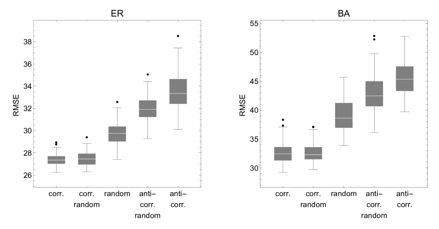
To compare the performance of these methods, we applied each of them to the same types of networks as used in Fig. 2. For each combination of two factor graphs and a method, we calculated the actual spectrum of $L_{G\times H}$ numerically, as well as the estimated spectrum using Eq. (42) with specific orderings of $\mu^{G}_{i}$ and $\mu^{H}_{j}$ determined by each ordering method. Both the actual and estimated spectra were sorted, and then each pair of actual and estimated eigenvalues were compared and their RMSE (root mean square error) was calculated across all eigenvalues, as the overall performance measure of each method.

Figure 3: Comparison of estimation performance (RMSE) among five ordering methods (see text for details of each method) for estimating Laplacian spectra of direct product graphs. Results were collected from one hundred independent tests for each condition, and their distributions were shown in box-whisker plots. Gray boxes show 25 percentiles above and below a mean, while whiskers show the whole range. Black dots indicate outliers. Left (“ER”): $G$ = Erdős-Rényi random graph with 50 nodes and 100 edges, and $H$ = Erdős-Rényi random graph with 30 nodes and 90 edges. Right (“BA”): $G$ = Barabási-Albert graph with 50 nodes and 2 edges per each newcomer node, and $H$ = Barabási-Albert graph with 30 nodes and 3 edges per each newcomer node. ANOVA and Tukey/Bonferroni posthoc tests showed highly significant differences among the conditions except between correlated ordering (“corr.”) and correlated ordering with randomization (“corr. random”).

Results are summarized in Fig. 3, which shows a clear trend for both Erdős-Rényi and Barabási-Albert factor graphs. The most effective ordering methods turned out to be correlated orderings (without and with randomization; there was no statistical difference between them). In contrast, anti-correlated orderings had an adverse effect on the estimation results. Based on this result, we adopted the correlated ordering, the simplest and best performing choice among the five methods tested.

Our final estimation method is summarized as follows:

Proposed method for estimating a Laplacian spectrum of a direct product graph

1. Obtain degree and Laplacian spectra of two factor graphs $G$ and $H$. We denote them as $d^{G}=\{d^{G}_{i}\}$, $d^{H}=\{d^{H}_{j}\}$, $\mu^{G}=\{\mu^{G}_{i}\}$ and $\mu^{H}=\{\mu^{H}_{j}\}$.

2. Sort all the spectra in an ascending order.

3. Calculate the following set for all $i=1,2,\ldots,|V_{G}|$ and $j=1,2,\ldots,|V_{H}|$:

   $$\mu^{G\times H}=\{\;\mu^{G}_{i}d^{H}_{j}+d^{G}_{i}\mu^{H}_{j}-\mu^{G}_{i}\mu^{H}_{j}\;\}$$

   $\mu^{G\times H}$ is the estimated Laplacian spectrum of $G\times H$.

The computational complexity of this method is $O(f(m)+f(n)+m\log m+n\log n+mn)$, where $m=|V_{G}|$, $n=|V_{H}|$, and $O(f(k))$ is the computational complexity of calculating degree and Laplacian spectra of a graph made of $k$ nodes. In general $O(f(k))=O(k^{3})$, so the complexity of this method is characterized by $O(m^{3}+n^{3}+m\log m+n\log n+mn)$. This is substantially smaller than $O(f(mn))=O(m^{3}n^{3})$, i.e., the complexity of explicit computation of eigenvalues of $L_{G\times H}$, especially when $m$ and $n$ are large.

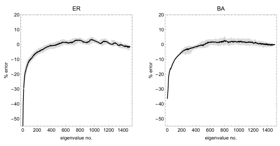
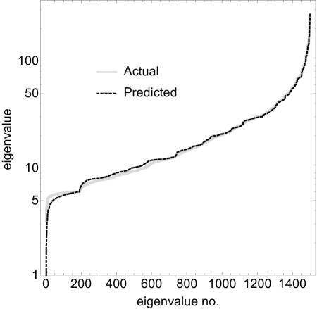
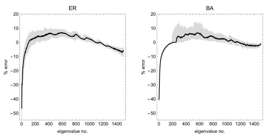
Figure 4 shows an example of a Laplacian spectrum of a direct product graph made of two Barabási-Albert graphs estimated using the proposed method. While there are some noticeable differences between the actual and estimated results, the overall profile of the spectrum is reasonably well captured. Figure 5 shows distributions of percentage errors of the estimated eigenvalues compared to the actual ones. The first eigenvalue was always matched at 0 in both actual and estimated spectra (because Eq. (42) guarantees this), but our method consistently underestimated the immediately following several eigenvalues (small ones) significantly. This is where the spectrum shows a drastic jump from 0 (see Fig. 4). In the meantime, the estimation errors for the remaining eigenvalues were mostly confined within a $\pm 10$% range for both Erdős-Rényi and Barabási-Albert cases. We consider this a reasonable estimation accuracy, given the drastic reduction of computational complexity achieved by our method. The characteristic shape of error profiles seen in Fig. 5, i.e., a sudden jump at the beginning followed by a gradual decrease, was fairly consistent across various network topologies we tested, so one might be able to develop a heuristic error reduction technique to further improve the accuracy of estimation (which we did not attempt within the scope of this paper).

Figure 4: An example of a Laplacian spectrum of a direct product graph estimated using the proposed method (black dashed curve) in comparison with the actual one (gray solid curve). Eigenvalues are sorted in an ascending order. $G$ = Barabási-Albert graph with 50 nodes and 2 edges per each newcomer node, and $H$ = Barabási-Albert graph with 30 nodes and 3 edges per each newcomer node.

Figure 5: Distributions of percentage errors in Laplacian spectra of direct product graphs estimated using the proposed method compared to actual ones. Results were collected from one hundred independent tests for each network topologies (“ER” and “BA”). Black curves show medians, and shaded areas show ranges from 5 to 95 percentiles. Left (“ER”): $G$ = Erdős-Rényi random graph with 50 nodes and 100 edges, and $H$ = Erdős-Rényi random graph with 30 nodes and 90 edges. Right (“BA”): $G$ = Barabási-Albert graph with 50 nodes and 2 edges per each newcomer node, and $H$ = Barabási-Albert graph with 30 nodes and 3 edges per each newcomer node. Smaller eigenvalues were typically underestimated significantly, while estimation errors for the rest were mostly confined within a $\pm 10$% range (96.5% of the eigenvalues for “ER” and 94.0% of the eigenvalues for “BA” are within this error range). This observation remains similar when the sizes of the graphs are varied (the percentage errors are smaller for larger graphs).

4.2 Estimating Laplacian spectra of strong product graphs

Finally, we extend the methodology we used in the previous section to estimate Laplacian spectra of strong product graphs. A Laplacian of strong product graph $G\boxtimes H$ is given as follows:

$$L_{G\boxtimes H} =D_{G\boxtimes H}-A_{G\boxtimes H}$$ (45)

$$=(D_{G\Box H}+D_{G\times H})-(A_{G\Box H}+A_{G\times H})$$ (46)

$$=(D_{G}\otimes I_{|V_{H}|}+I_{|V_{G}|}\otimes D_{H}+D_{G}\otimes D_{H})-(A_{G}\otimes I_{|V_{H}|}+I_{|V_{G}|}\otimes A_{H}+A_{G}\otimes A_{H})$$ (47)

$$=D_{G}\otimes I_{|V_{H}|}+I_{|V_{G}|}\otimes D_{H}+D_{G}\otimes D_{H}$$

$$\quad\quad\quad-(D_{G}-L_{G})\otimes I_{|V_{H}|}-I_{|V_{G}|}\otimes(D_{H}-L_{H})-(D_{G}-L_{G})\otimes(D_{H}-L_{H})$$ (48)

$$=L_{G}\otimes I_{|V_{H}|}+I_{|V_{G}|}\otimes L_{H}+L_{G}\otimes D_{H}+D_{G}\otimes L_{H}-L_{G}\otimes L_{H}$$ (49)

As seen above, the only change from the direct product Laplacian (Eq. (33)) is the inclusion of the first two terms ($L_{G}\otimes I_{|V_{H}|}$ and $I_{|V_{G}|}\otimes L_{H}$), each of which has $w^{G}_{i}\otimes w^{H}_{j}$ as its eigenvector (this can be easily shown). Therefore we can still use the same strategy to use $w^{G}_{i}\otimes w^{H}_{j}$ as a reasonable substitute of the true eigenvectors of $L_{G\boxtimes H}$. We calculate $L_{G\boxtimes H}(w^{G}_{i}\otimes w^{H}_{j})$ as follows:

$$L_{G\boxtimes H}(w^{G}_{i}\otimes w^{H}_{j}) =(L_{G}\otimes I_{|V_{H}|}+I_{|V_{G}|}\otimes L_{H}+L_{G}\otimes D_{H}+D_{G}\otimes L_{H}-L_{G}\otimes L_{H})(w^{G}_{i}\otimes w^{H}_{j})$$ (50)

$$=\mu^{G}_{i}w^{G}_{i}\otimes w^{H}_{j}+w^{G}_{i}\otimes\mu^{H}_{j}w^{H}_{j}+\mu^{G}_{i}w^{G}_{i}\otimes D_{H}w^{H}_{j}+D_{G}w^{G}_{i}\otimes\mu^{H}_{j}w^{H}_{j}-\mu^{G}_{i}w^{G}_{i}\otimes\mu^{H}_{j}w^{H}_{j}$$ (51)

Using the same aggregate notation and the heuristic assumption, this becomes

$$L_{G\boxtimes H}(W_{G}\otimes W_{H}) =W_{G}M_{G}\otimes W_{H}+W_{G}\otimes W_{H}M_{H}+W_{G}M_{G}\otimes D_{H}W_{H}+D_{G}W_{G}\otimes W_{H}M_{H}-W_{G}M_{G}\otimes W_{H}M_{H}$$ (52)

$$\approx W_{G}M_{G}\otimes W_{H}+W_{G}\otimes W_{H}M_{H}+W_{G}M_{G}\otimes W_{H}D_{H}+W_{G}D_{G}\otimes W_{H}M_{H}-W_{G}M_{G}\otimes W_{H}M_{H}$$ (53)

$$=(W_{G}\otimes W_{H})\bigg{(}M_{G}+M_{H}+M_{G}\otimes D_{H}+D_{G}\otimes M_{H}-M_{G}\otimes M_{H}\bigg{)},$$ (54)

where inside the second pair of parentheses is a diagonal matrix whose diagonal entries show a hypothetical spectrum:

$$\{\;\mu^{G}_{i}+\mu^{H}_{j}+\mu^{G}_{i}d^{H}_{j}+d^{G}_{i}\mu^{H}_{j}-\mu^{G}_{i}\mu^{H}_{j}\;\}$$ (55)

Numerical experiments showed that the correlated ordering is still most effective in this case too (results not shown). Our proposed method for strong product graphs can thus be summarized as follows:

Proposed method for estimating a Laplacian spectrum of a strong product graph

1. Obtain degree and Laplacian spectra of two factor graphs $G$ and $H$. We denote them as $d^{G}=\{d^{G}_{i}\}$, $d^{H}=\{d^{H}_{j}\}$, $\mu^{G}=\{\mu^{G}_{i}\}$ and $\mu^{H}=\{\mu^{H}_{j}\}$.

2. Sort all the spectra in an ascending order.

3. Calculate the following set for all $i=1,2,\ldots,|V_{G}|$ and $j=1,2,\ldots,|V_{H}|$:

   $$\mu^{G\boxtimes H}=\{\;\mu^{G}_{i}+\mu^{H}_{j}+\mu^{G}_{i}d^{H}_{j}+d^{G}_{i}\mu^{H}_{j}-\mu^{G}_{i}\mu^{H}_{j}\;\}$$

   $\mu^{G\boxtimes H}$ is the estimated Laplacian spectrum of $G\boxtimes H$.

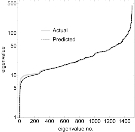
The computational complexity is the same as that of the method for direct product graphs. An example of an estimated Laplacian spectrum and the distributions of percentage errors are shown in Figs. 6 and 7, respectively.

Figure 6: An example of a Laplacian spectrum of a strong product graph estimated using the proposed method (black dashed curve) in comparison with the actual one (gray solid curve). Eigenvalues are sorted in an ascending order. $G$ = Barabási-Albert graph with 50 nodes and 2 edges per each newcomer node, and $H$ = Barabási-Albert graph with 30 nodes and 3 edges per each newcomer node.

Figure 7: Distributions of percentage errors in Laplacian spectra of strong product graphs estimated using the proposed method compared to actual ones. Results were collected from one hundred independent tests for each network topologies (“ER” and “BA”). Black curves show medians, and shaded areas show ranges from 5 to 95 percentiles. Left (“ER”): $G$ = Erdős-Rényi random graph with 50 nodes and 100 edges, and $H$ = Erdős-Rényi random graph with 30 nodes and 90 edges. Right (“BA”): $G$ = Barabási-Albert graph with 50 nodes and 2 edges per each newcomer node, and $H$ = Barabási-Albert graph with 30 nodes and 3 edges per each newcomer node. Smaller eigenvalues were typically underestimated significantly, while estimation errors for the rest were mostly confined within a $\pm 10$% range (92.9% of the eigenvalues for “ER” and 92.8% of the eigenvalues for “BA” are within this error range). This observation remains similar when the sizes of the graphs are varied (the percentage errors are smaller for larger graphs).

5 Conclusions

In this paper, we have developed and evaluated computationally plausible methods for estimating Laplacian spectra of direct and strong product graphs, for which there is no known exact formulas to date. Our methods were designed using a few mathematically incorrect assumptions, yet the results were generally in reasonable agreement with the explicitly computed spectra with percentage errors confined within a $\pm 10$% range for most eigenvalues. The computational complexity of the proposed methods is orders of magnitude smaller than that of explicit computation of eigenvalues of a product graph, especially when the factor graphs are large. This suggests that, if one could approximate the topology of a large-scale network by a Cartesian, direct, or strong product of two (or more) factor graphs, the Laplacian spectrum of the network might be estimated efficiently using our methods. Designing and evaluating such graph factorization and spectral estimation algorithms will be an important direction of future research.

The present study still has many fundamental limitations to which we need to call readers’ attention. The most fundamental problem is that we have not yet come up with a rigorous mathematical explanation of why and how the proposed methods work. We used heuristics at several steps in designing the methods without much theoretical support. Second, the outputs produced by our methods are nothing more than crude estimates, which wouldn’t even converge to true spectra even if the eigenvalue orderings were completely optimized (we confirmed this through numerical experiments conducting exhaustive search for optimal orderings for small-sized factor graphs). The percentage errors were particularly large for small eigenvalues, which are often more important in spectral graph theory and network analysis (e.g., algebraic connectivity [4]). Finally, we used random graphs (Erdős-Rényi and Barabási-Albert graphs) in the evaluations, so there is no assurance about the behavior of our methods on graphs with very specific non-random topologies whose Laplacians show peculiar properties. In view of all of these limitations, the proposed methods should be considered more as initial “working hypotheses” for promoting further theoretical investigation and algorithm development, rather than immediately useful algorithms for practical problem solving.

References

• [1] Sasmita Barik, Ravindra B Bapat, and S Pati. On the laplacian spectra of product graphs. Applicable Analysis and Discrete Mathematics, 9:39–58, 2015.
• [2] Stefano Boccaletti, G Bianconi, R Criado, Charo I Del Genio, J Gómez-Gardeñes, M Romance, I Sendina-Nadal, Z Wang, and M Zanin. The structure and dynamics of multilayer networks. Physics Reports, 544(1):1–122, 2014.
• [3] Manlio De Domenico, Albert Solé-Ribalta, Emanuele Cozzo, Mikko Kivelä, Yamir Moreno, Mason A Porter, Sergio Gómez, and Alex Arenas. Mathematical formulation of multilayer networks. Physical Review X, 3(4):041022, 2013.
• [4] Miroslav Fiedler. Algebraic connectivity of graphs. Czechoslovak Mathematical Journal, 23(2):298–305, 1973.
• [5] Richard Hammack, Wilfried Imrich, and Sandi Klavžar. Handbook of Product Graphs. CRC press, 2011.
• [6] Wilfried Imrich and Janez Žerovnik. Factoring cartesian-product graphs. Journal of Graph Theory, 18(6):557–567, 1994.
• [7] A Kaveh and B Alinejad. Laplacian matrices of product graphs: applications in structural mechanics. Acta mechanica, 222(3-4):331–350, 2011.
• [8] A Kaveh and H Rahami. Block diagonalization of adjacency and Laplacian matrices for graph product; applications in structural mechanics. International Journal for Numerical Methods in Engineering, 68(1):33–63, 2006.
• [9] Mikko Kivelä, Alex Arenas, Marc Barthelemy, James P Gleeson, Yamir Moreno, and Mason A Porter. Multilayer networks. Journal of Complex Networks, 2(3):203–271, 2014.
• [10] Jure Leskovec, Deepayan Chakrabarti, Jon Kleinberg, Christos Faloutsos, and Zoubin Ghahramani. Kronecker graphs: An approach to modeling networks. The Journal of Machine Learning Research, 11:985–1042, 2010.
• [11] Jure Leskovec and Christos Faloutsos. Scalable modeling of real graphs using Kronecker multiplication. In Proceedings of the 24th international conference on Machine learning, pages 497–504. ACM, 2007.
• [12] Jurij Leskovec, Deepayan Chakrabarti, Jon Kleinberg, and Christos Faloutsos. Realistic, mathematically tractable graph generation and evolution, using Kronecker multiplication. In Knowledge Discovery in Databases: PKDD 2005, pages 133–145. Springer, 2005.
• [13] Cyrus Colton MacDuffee. The Theory of Matrices. Springer-Verlag, 1933.
• [14] Gert Sabidussi. Graph multiplication. Mathematische Zeitschrift, 72(1):446–457, 1959.
• [15] Rubén J Sánchez-García, Emanuele Cozzo, and Yamir Moreno. Dimensionality reduction and spectral properties of multilayer networks. Physical Review E, 89(5):052815, 2014.
• [16] Hiroki Sayama. Dynamics of graph product multilayer networks. in preparation.
• [17] Albert Solé-Ribalta, Manlio De Domenico, Nikos E Kouvaris, Albert Díaz-Guilera, Sergio Gómez, and Alex Arenas. Spectral properties of the Laplacian of multiplex networks. Physical Review E, 88(3):032807, 2013.