A Simple and Effective High-Order Shock-Capturing Limiter for Discontinuous Galerkin Methods

Abstract

The discontinuous Galerkin (DG) finite element method when applied to hyperbolic conservation laws requires the use of shock-capturing limiters in order to suppress unphysical oscillations near large solution gradients. In this work we develop a novel shock-capturing limiter that combines key ideas from the limiter of Barth and Jespersen [AIAA-89-0366 (1989)] and the maximum principle preserving (MPP) framework of Zhang and Shu [Proc. R. Soc. A, 467 (2011), pp. 2752–2776]. The limiting strategy is based on traversing the mesh element-by-element in order to (1) find local upper and lower bounds on user-defined variables by sampling these variables on neighboring elements, and (2) to then enforce these local bounds by minimally damping the high-order corrections. The main advantages of this limiting strategy is that it is simple to implement, effective at shock capturing, and retains high-order accuracy of the solution in smooth regimes. The resulting numerical scheme is applied to several standard numerical tests in both one and two-dimensions and on both Cartesian and unstructured grids. These tests are used as benchmarks to verify and assess the accuracy and robustness of the method.

siscxxxxxxxx–x

1 Introduction

1.1 Some background

Godunov’s theorem [7] states that a linear numerical method when applied to the one-dimensional, linear, advection equation:

(1) $$\frac{\partial q}{\partial t}+\frac{\partial q}{\partial x}=0,\quad q(t=0,x)=q_{0}(x),$$

where $x\in\mathbb{R}$, $t\in\mathbb{R}_{\geq 0}$, and $q(t,x):\mathbb{R}_{\geq 0}\times\mathbb{R}\rightarrow\mathbb{R}$, is monotone (i.e., does not generate new extrema) only if it is at most first-order accurate. In practice, schemes that are not monotone will exhibit large spurious oscillations near discontinuities in the solution. The analog of this result for more complicated hyperbolic equations (i.e., nonlinear systems in multiple dimensions) is that linear numerical methods with a formal accuracy higher than first-order will create spurious oscillations that can lead to catastrophic numerical instabilities (e.g., negative densities and/or pressures). As in the linear scalar case, these instabilities are especially pronounced if the solution becomes discontinuous (i.e., shock waves and contact discontinuities). The additional challenge with nonlinear hyperbolic equations is that generic initial conditions tend to produce shocks in finite time.

The principal remedy for these numerical instabilities in high-order methods is to introduce a shock-capturing limiter; such limiters render an otherwise linear method nonlinear, thereby circumventing the restrictions of Godunov’s theorem. Typically, limiters are designed to execute two tasks: (1) to monitor the solution quality (at least in some simplified sense); and, when necessary, (2) to reduce the influence of high-order corrections. The development of limiters for hyperbolic equations was pioneered by Bram van Leer in a series of papers starting with [40, 41]. Additional fundamental contributions came from Harten [9, 10], Sweby [38], and Tadmor [39] who developed mathematical precise limiting strategies based on the principle that the numerical scheme should be total variation non-increasing. A good review of these limiters can be found in Chapter 6 of LeVeque [22]. In more recent work, many contributions have been made to generalize these limiting strategies to high-order methods, including to weighted non-oscillatory (WENO) schemes (e.g., see Liu et al. [23] and Jiang and Shu [14] ) and discontinuous Galerkin schemes (e.g., for a review see Qiu and Shu [28] and Dumbser et al. [6]).

In this work we focus on limiters for discontinuous Galerkin (DG) methods [31, 3, 4]. Limiting strategies for DG methods can generally be broken down into two key steps:

Step 1.

Detect troubled-cells (i.e., cells that contain large gradients);

Step 2.

Apply a limiter to each troubled cell that is detected (i.e., in some way reduce the local gradients or higher derivative analogs thereof without changing the average value in that cell).

In some limiting strategies these two steps are executed with completely different techniques (e.g., see [28]), while in other approaches the detection and limiting happen in all in one fell swoop (e.g., the moment limiter of Krivodonova [16]). In either case, the end goal of most limiters is to design a method that simultaneously accomplishes two often conflicting objectives: (1) reduce unphysical oscillations in the presence of shocks and (2) retain high-order accuracy in smooth regimes.

The techniques used for DG methods in the limiting step (Step 2) can be subdivided into three broad classes of limiters, which we briefly describe below.

1.1.1 Moment or slope methods

These limiters have their roots in the development of classical second-order finite volume methods. The key ingredients are minimum modulus evaluations that compare the slope (or higher derivative analogs) in the current cell to values computed from neighboring cells. Such methods are still widely used (e.g., see [12, 13, 16, 44, 18, 19, 20]). There are two well-known difficulties with these limiters: (1) they tend to degrade the of order of accuracy in smooth extrema; and (2) they are difficult to generalize to unstructured meshes.

1.1.2 Hybrid weighted essentially non-oscillatory methods

Methods in this category are motivated by the success of the weighted essentially non-oscillatory (WENO) method in shock-capturing. The classical schemes [27, 29, 30, 50, 48, 49, 51] redefine the polynomial representation of the solution inside each element by considering neighboring elements and matching cell averages. The WENO reconstruction, which is automatically mass conservative, is then typically applied in order to redefine polynomial representations inside each element. More recently, the so-called Hermite WENO schemes have been used in an effort to reduce the size of the computational stencil [24]. A chief criticism of these methods has been the expense of their application; although recent efforts exist to reduce their computational cost [51].

1.1.3 Artificial viscosity methods

This method is based on the classical idea of adding a small amount of artificial viscosity to hyperbolic equations [42]. The modern incarnation of this limiting strategy was pioneered by Persson and Peraire [26] and further developed in [45, 1]. These methods typically work by using a smoothness indicator to first detect troubled cells, and then directly discretizing a diffusive term that has been artificially added to the equations in an effort to smooth-out oscillations. One drawback of using these limiters with explicit time-stepping schemes is that due to the diffusion operator, the maximum stable time-step is $\Delta t=\mathcal{O}(h/{M^{2}_{\text{D}}})$ (i.e., the viscosity parameter is typically $\mathcal{O}(h)$), where $h$ is the grid spacing and ${M_{\text{D}}}$ is the highest polynomial order of the basis polynomials, rather than the typical $\Delta t=\mathcal{O}(h/{M_{\text{D}}})$ for hyperbolic systems.

Other variations such as minimum entropy satisfying limiters [47] have also begun to be investigated. A complete description of what options exist for limiting DG solutions is beyond the scope of this work; we direct the interested reader to [6] for a recent and extensive review of the literature.

1.2 Brief summary of current work

The purpose of this work is to develop a novel limiter for discontinuous Galerkin methods that has all of the following properties:

• Provable high-order accuracy in smooth regimes;

• Robust reduction in spurious oscillations in the presence of shocks;

• Computationally efficient (i.e., only uses neighboring cells and no characteristic decompositions);

• Easy to implement in existing DG codes;

• Automatic extension to multidimensional settings including Cartesian and unstructured grids; and

• Automatic incorporation of positivity preserving limiters.

The limiter presented in this work can be viewed as a novel extension of two separate methods. First, it can be thought of as extending the finite volume Barth-Jespersen limiter [2] to the discontinuous Galerkin framework. Second, it can be viewed as an extension of the modern maximum principle preserving DG schemes developed by Zhang and Shu [46]. In particular, the limiter is based on finding for each element local upper and lower bounds using only nearest neighbor values, and then limiting the higher-order modes in such a way that that mass conservation is automatic and such that the limited solution remains within the predicted local bounds. Roughly speaking, this limiter can be viewed as belonging to the moment or slope methods, although it has important differences with the current methods in this class, including no need to for characteristic decompositions, no need for hierarchical highest-to-lowest moment limiting, and easy extensibility to unstructured meshes.

The remainder of this paper is organized as follows. In Section 2 we briefly review the DG method. The basic limiting strategy for a one-dimensional scalar equation is outlined in Section 3. In Section 4 we describe how the proposed limiter obtains high-order accuracy. Extension to multiple dimensions is shown in Section 5 and to general systems of hyperbolic conservation laws in Section 6, where we use the compressible Euler equations as the prototypical example. In Section 7 we describe how positivity-preserving ideas can be incorporated. The numerical method is validated on several standard cases for the compressible Euler equations in Section 8. Conclusions are made in Section 9.

1.3 Implementation details

All of the numerical examples carried out in this work are implemented in the software package DoGPack [32]. This software package is open-source and all the code used in this work can be freely downloaded from the web.

2 DG-FEM framework

In order to define the proposed limiter, we first provide a brief description of the discontinuous Galerkin (DG) method, which serves to define the notation used throughout the remainder of this work. We refer the interested reader to [4, 11, 36] and references therein for further details of the DG method.

Consider a conservation law of the form

(2) $$q_{,t}+{\nabla}\cdot{\bf F}(q)=0,\quad\text{in}\,\,\,\Omega\subset\mathbb{R}^{d},$$

with appropriate boundary conditions, where $q(t,{\bf x}):\mathbb{R}_{\geq 0}\times\mathbb{R}^{d}\mapsto\mathbb{R}^{{M_{\text{E}}}}$ are the conserved variables, ${\bf F}(q):\mathbb{R}^{{M_{\text{E}}}}\mapsto\mathbb{R}^{{M_{\text{E}}}\times d}$ is the flux function, $d$ is the spatial dimension, and ${M_{\text{E}}}$ is the number of equations in the system. We assume that the system is hyperbolic, meaning that the flux Jacobian matrix, ${\bf n}\cdot{\bf F}_{,q}$, is diagonalizable with real eigenvalues for all $q$ in the domain of interest and for all $\|{\bf n}\|=1$.

Let $\Omega\subset\mathbb{R}^{d}$ be a polygonal domain with boundary $\partial\Omega$. The domain $\Omega$ is discretized via a finite set of non-overlapping elements, $\mathcal{T}_{i}$, such that $\Omega=\cup_{i=1}^{N}\mathcal{T}_{i}$. Let ${P}^{\,{M_{\text{D}}}}\left(\mathbb{R}^{d}\right)$ denote the set of polynomials from $\mathbb{R}^{d}$ to $\mathbb{R}$ with maximal polynomial degree ${M_{\text{D}}}$. Let ${\mathcal{W}}^{h}$ denote the broken finite element space on the mesh:

(3) $${\mathcal{W}}^{h}:=\left\{w^{h}\in\left[L^{\infty}(\Omega)\right]^{{M_{\text{E}}}}:\,w^{h}\bigl{|}_{\mathcal{T}_{i}}\in\left[{P}^{\,{M_{\text{D}}}}\right]^{{M_{\text{E}}}},\,\forall\mathcal{T}_{i}\in\mathcal{T}^{h}\right\},$$

where $h$ is the grid spacing. The above expression means that $w^{h}\in{\mathcal{W}}^{h}$ has ${M_{\text{E}}}$ components, each of which when restricted to some element $\mathcal{T}_{i}$ is a polynomial of degree at most ${M_{\text{D}}}$ and no continuity is assumed across element edges (or faces in 3D).

The approximate solution on each element $\mathcal{T}_{i}$ at time $t=t^{n}$ is of the form

(4) $$q^{h}(t^{n},{\bf x}(\bm{\xi}))\Bigl{|}_{\mathcal{T}_{i}}=\sum_{\ell=1}^{{M_{\text{L}}}({M_{\text{D}}})}\,Q^{(\ell)n}_{i}\,\varphi^{(\ell)}\left(\bm{\xi}\right),$$

where ${M_{\text{L}}}$ is the number of Legendre polynomials and $\varphi^{(\ell)}\left(\bm{\xi}\right):\mathbb{R}^{d}\mapsto\mathbb{R}$ are the Legendre polynomials defined on the reference element ${\mathcal{T}}_{0}$ in terms of the reference coordinates $\bm{\xi}\in\mathcal{T}_{0}$. The Legendre polynomials are orthonormal with respect to the following inner product:

(5) $$\frac{1}{|\mathcal{T}_{0}|}\int_{\mathcal{T}_{0}}\varphi^{(k)}(\bm{\xi})\,\varphi^{(\ell)}(\bm{\xi})\,d\bm{\xi}=\begin{cases}1&\,\text{if}\quad k=\ell,\\ 0&\,\text{if}\quad k\neq\ell.\end{cases}$$

We note that independent of $h$, $d$, ${M_{\text{D}}}$, and the type of element, the lowest order Legendre polynomial is always $\varphi^{(1)}\equiv 1$. This makes the first Legendre coefficient the cell average:

(6) $$Q^{(1)n}_{i}=\frac{1}{|\mathcal{T}_{0}|}\int_{\mathcal{T}_{0}}q^{h}(t^{n},{\bf x}(\bm{\xi}))\Bigl{|}_{\mathcal{T}_{i}}\,\varphi^{(1)}\left(\bm{\xi}\right)\,d\bm{\xi}=:\bar{q}^{n}_{i}.$$

To obtain the semi-discrete DG method, equation (2) is multiplied by the test function $\varphi^{(k)}$, the resulting equation is integrated over an element $\mathcal{T}_{i}$, and integrations-by-part are performed on the flux term. The result is the following system of ODEs:

(7) $$\dot{Q}^{(k)}_{i}=\frac{1}{|\mathcal{T}_{i}|}\int_{\mathcal{T}_{i}}\nabla_{\bf x}\varphi^{(k)}\cdot{\bf F}\left(q^{h}\Bigl{|}_{\mathcal{T}_{i}}\right)\,d{\bf x}-\frac{1}{|\mathcal{T}_{i}|}\oint_{\partial_{\mathcal{T}_{i}}}\varphi^{(k)}{\mathcal{F}}\cdot d{\bf s},$$

where the numerical fluxes ${\mathcal{F}}$ must be determined via (approximate) Riemann solvers. In this work we make use of the Rusanov [33] numerical flux, which is often referred to as the local Lax-Friedrichs (LLF) flux in the literature.

Finally, in order to obtain a Runge-Kutta DG method, equation (7) is discretized in time via some Runge-Kutta method. In this work we make use of strong stability-preserving (SSP) Runge-Kutta methods, such as those found in Gottlieb, Shu, and Tadmor [8] and Ketcheson [15].

3 Proposed limiter: The scalar case

The basic procedure we follow to limit the solution on a single element $\mathcal{T}_{i}$ is given by the following sequence of steps:

Step 0.

Define a set of points $\chi_{i}$ that will be used to approximate cell maximum and minimum values. In the current work, we use Gaussian quadrature nodes and augment them with corner points and quadrature points along the element boundaries (i.e., edge Gaussian quadrature points).

Step 1.

For each mesh element, $\mathcal{T}_{i}$, we compute an approximate maximum and minimum:

$$q_{M_{i}}:=\max_{x\in\chi_{i}}\left\{q^{h}(x)\Bigl{|}_{\mathcal{T}_{i}}\right\}\quad\text{and}\quad q_{m_{i}}:=\min_{x\in\chi_{i}}\left\{q^{h}(x)\Bigl{|}_{\mathcal{T}_{i}}\right\}.$$

Step 2.

We consider the set $N_{\mathcal{T}_{i}}$ of all neighbors of $\mathcal{T}_{i}$, excluding $\mathcal{T}_{i}$ itself, and compute an approximate upper and lower bound:

(8) $$M_{i}:= \max\left\{\bar{q}_{i}+\alpha(h),\,\,\max_{j\in N_{\mathcal{T}_{i}}}\left\{q_{M_{j}}\right\}\right\},$$

(9) $$m_{i}:= \min\left\{\bar{q}_{i}-\alpha(h),\,\,\min_{j\in N_{\mathcal{T}_{i}}}\left\{q_{m_{j}}\right\}\right\}.$$

The scalar function $\alpha(h)\geq 0$ is a tolerance function that will be described shortly. The most aggressive limiter we consider sets $\alpha=0$.

Step 3.

We define

(10) $$\theta_{M_{i}}:=\phi\left(\frac{M_{i}-\bar{q}_{i}}{q_{M_{i}}-\bar{q}_{i}}\right)\quad\text{and}\quad\theta_{m_{i}}:=\phi\left(\frac{m_{i}-\bar{q}_{i}}{q_{m_{i}}-\bar{q}_{i}}\right),$$

where $0\leq\phi(y)\leq 1$ is a cutoff function. In this work, we use the function

(11) $$\phi(y):=\min\left\{\frac{y}{1.1},1\right\},$$

which is motivated by the work of [25]. The form of this function becomes important in the multidimensional setting, which will be described shortly.

Step 4.

We define the rescaling parameter as

(12) $$\theta_{i}:=\min\left\{1,\ \theta_{m_{i}},\ \theta_{M_{i}}\right\}.$$

Step 5.

Finally, we rescale the approximate solution on the element $\mathcal{T}_{i}$ as

(13) $$\tilde{q}^{h}(x)\Bigl{|}_{\mathcal{T}_{i}}:=\bar{q}_{i}+\theta_{i}\left(q^{h}(x)\Bigl{|}_{\mathcal{T}_{i}}-\bar{q}_{i}\right).$$

Before delving into the finer details of the method, a few remarks are in order.

Remark 1.

The choice of quadrature points in Step 1 is not unique.

Indeed, the purpose of this step is to construct an approximate upper and lower bound for the solution. We originally tested this limiter by using cell averages, but found that those solutions tended to be quite diffusive near shocks. Directly sampling neighboring cells (that are potentially oscillating) allows us to retain sharper features in the solution.

Remark 2.

The presence of a non-zero value of $\alpha$ in Step 3 is required to obtain high-order accuracy at local extrema.

This issue will be elaborated upon in Section 4.

Remark 3.

When the proposed scheme is compared to the recent maximum principle preserving (MPP) limiters [46], significant differences come into play in Step 2 and Step 3.

• For the MPP methods, Step 2 is replaced by fixed a priori global bounds, whereas we follow the Barth-Jespersen idea [2] and use this step to estimate local upper and lower bounds for the solution.

• In Step 3, the MPP limiters use hard upper and lower bounds for the solution that are known a priori, whereas we use the result from Step 2 to estimate these.

• In the MPP literature, authors normally set $\phi(y)=\min\{1,y\}$, whereas we find that the form of this function is important when pushing to multiple dimensions. In Section 5 we elaborate on this idea.

Additionally, the newly proposed limiter is designed to capture shocks, whereas the original MPP limiter for DG methods was solely designed to preserve the maximum principle property of hyperbolic problems. In their work, additional limiting was necessary in order to suppress unphysical oscillations.

Remark 4.

The rescaling in Step 6 does not effect the total mass.

The consequence of this is that the limiter will be automatically mass conservative, which is an important property for hyperbolic solvers. This can be observed by simply integrating equation (13) over a single element.

4 On the importance of $\alpha$ for retaining high-order accuracy

In this section we describe the importance of $\alpha$ for obtaining a method that is genuinely high-order accurate. Many limiters exhibit the so-called “clipping” phenomenon, where smooth extrema are cut off because the limiter turns on and damps out these values. Recent efforts have been put forth to mitigate this clipping phenomenon for other discretizations, including the piecewise parabolic method (PPM) [5].

In this section, we will argue that high-order accuracy will be retained provide that the scalar function $\alpha\left(h\right):\mathbb{R}_{\geq 0}\to\mathbb{R}_{\geq 0}$ vanishes slower than $\mathcal{O}(h^{2})$. This observation was inspired by recent work on extensions of the Barth-Jespersen limiter to finite volume methods [25], and we demonstrate the performance of our limiter by testing it on a smooth solution in 1D.

In one dimension we can break down any smooth function on a bounded domain into monotonic regions and finitely many points of local extrema. We begin with a discussion of monotonic regions, and then turn to isolated local extrema.

4.1 Performance in monotonic regions

In regions where the exact solution is monotonic, the proposed limiter does not effect the asymptotic convergence rate independent of the choice of $\alpha\geq 0$. Without loss of generality, we consider a region with the solution is non-decreasing. After after enough refinement, the exact solution satisfies $q_{i-1}\leq q_{i}\leq q_{i+1}$ where $q_{i}$ refers to the solution value on the $i^{\text{th}}$-grid cell in a monotonic region. The algorithm then correctly selects $q_{i+1}$ as an upper bound, $q_{i-1}$ as a lower bound, and therefore does not overreach by over limiting the solution on the $i^{\text{th}}$ grid cell. A formal proof of the order of accuracy would follow that already presented in [46], but would start with the fact that our algorithm over-estimates the upper bound and under-estimates the lower bound for the exact solution.

4.2 Performance in regions near smooth extrema

In this subsection, we describe the importance of using a non-zero value of $\alpha$ to maintain genuine high-order accuracy. If $\alpha$ is chosen to be too large, then oscillations in a given cell will never be clamped down, whereas if $\alpha$ vanishes too quickly, then smooth extrema will be clipped. Our goal is to find necessary conditions for maintaining high-order accuracy at smooth extrema.

To begin, we consider a Taylor expansion of a smooth function $q:\mathbb{R}\to\mathbb{R}$ at an extrema $x=\xi_{0}$:

$$q(x)=q({\xi_{0}})+q^{\prime}(\xi_{0})(x-\xi_{0})+\frac{1}{2}q^{\prime\prime}(\xi_{0})(x-\xi_{0})^{2}+\cdots.$$

Given that $q^{\prime}(\xi_{0})=0$, we observe that asymptotically $\left|q(x)-q({\xi_{0}})\right|=\mathcal{O}(h^{2})$ if $\left|x-{\xi_{0}}\right|=\mathcal{O}(h)$. This leads us to consider functions of the form $\alpha(h)=\mathcal{O}(h^{r})$, where $r<2$ in order to maintain

$$|q(x)-q({\xi_{0}})|=\mathcal{O}(h^{2})\leq|\alpha(h)|\quad\text{for all}\quad|x-\xi_{0}|=\mathcal{O}(h).$$

Note that in the 2D Cartesian case: $h=\text{max}\left(\Delta x,\,\Delta y\right)$, where $\Delta x$ and $\Delta y$ are the mesh widths in each coordinate direction.

That is, as long as $\alpha(h)$ goes to zero slow enough, then our limiter will eventually turn off and not clip smooth extrema. However, if we were to set $\alpha=0$, then our limiter will induce clipping at smooth extrema, and yet if $\alpha$ does not vanish as $h\rightarrow 0$, then our method would permit problematic oscillations to persist.

The choice of $\alpha$ is not unique, and if desired, could be tuned for any given problem. The trade-off is that if $\alpha$ is too large, then true oscillations will only be damped provided the mesh is fine enough. Our choice of $\alpha(h)=\mathcal{O}(h^{1.5})$ is consistent with the recommended switches that turn off similar Barth-Jespersen type limiters for finite volume schemes [25]. Extensive numerical tests indicate this choice finds a good balance between the need to limit near shocks, while being soft enough to allow high-order accuracy on coarse grids. In the case of smooth problems, our limited solution will always converge to the unlimited solution even near local extrema. We illustrate this point with a simple case study.

4.3 On the importance of $\alpha$: A simple 1D case study

We analyze the performance of the proposed limiter on the linear advection equation (1) on $x\in[0,1]$ with periodic boundary conditions and with the initial condition

(14) $$q(x)=\begin{cases}\cos^{6}\left(\frac{(x-0.5)\pi}{0.16}\right)\quad&\text{if }|x-0.5|<0.08,\\ 0\quad&\text{otherwise}.\end{cases}$$

In Table 1 we present a convergence study for various grid resolutions after advecting the solution through one full period (e.g., solve to $t=1$). For this example we use the $10$-stage SSP fourth-order Runge-Kutta scheme (SSPRK4) developed by Ketcheson [15] and hold a constant CFL number of $0.4$. We compare the results for the unlimited solution, the solution with $\alpha=0$, and the solution with $\alpha(h)=50h^{1.5}$.

We observe that after enough refinement, the limited and unlimited solutions agree with each other, whereas for very coarse grids, the order of accuracy is slightly degraded. It is only after the limiter “turns off” that we we dial in on high-order accuracy. This cutoff point is a function of the curvature of the exact solution at the local extrema. This example serves to illustrate that after enough refinement, there is no difference between the limited and unlimited solutions.

Mesh	No Limiter	Order	$\alpha=0$	Order	$\alpha=50h^{1.5}$	Order
$5$	$3.78\times 10^{-01}$	—	$8.73\times 10^{-01}$	—	$3.78\times 10^{-01}$	—
$8$	$5.61\times 10^{-01}$	$-0.84$	$9.00\times 10^{-01}$	$-0.07$	$5.61\times 10^{-01}$	$-0.84$
$14$	$2.32\times 10^{-01}$	$1.58$	$8.22\times 10^{-01}$	$0.16$	$2.34\times 10^{-01}$	$1.56$
$24$	$5.38\times 10^{-02}$	$2.71$	$7.04\times 10^{-01}$	$0.29$	$1.74\times 10^{-01}$	$0.56$
$42$	$4.24\times 10^{-03}$	$4.54$	$4.78\times 10^{-01}$	$0.69$	$7.82\times 10^{-02}$	$1.43$
$73$	$3.65\times 10^{-04}$	$4.44$	$2.24\times 10^{-01}$	$1.38$	$2.19\times 10^{-02}$	$2.30$
$127$	$3.89\times 10^{-05}$	$4.04$	$8.84\times 10^{-02}$	$1.68$	$2.73\times 10^{-03}$	$3.76$
$222$	$4.10\times 10^{-06}$	$4.03$	$2.97\times 10^{-02}$	$1.95$	$4.10\times 10^{-06}$	$11.64$
$388$	$4.38\times 10^{-07}$	$4.01$	$9.37\times 10^{-03}$	$2.07$	$4.38\times 10^{-07}$	$4.01$
$679$	$4.65\times 10^{-08}$	$4.01$	$2.76\times 10^{-03}$	$2.19$	$4.65\times 10^{-08}$	$4.01$

Table 1: Convergence for the 1D advection problem in Section 4.3. All errors are $L_{2}$ norm errors. We see that a nonzero value of $\alpha$ is required to allow the limiting to completely turn off when the solution is properly resolved.

5 On the importance of $\phi$ for multidimensional cases

An important distinction between the single and multidimensional cases is that in higher dimensions, shocks are no longer isolated to single cells. To illustrate this, consider the following initial condition:

(15) $$q(x,y)=\begin{cases}1,&\text{if }x\leq 0,\\ 0,&\text{otherwise}.\end{cases}$$

Now, consider a Cartesian mesh with cells of width $\Delta x$ and height $\Delta y$:

(16) $$C_{ij}:=\left[\left(i-\frac{1}{2}\right)\Delta x,\left(i+\frac{1}{2}\right)\Delta x\right]\times\left[\left(j-\frac{1}{2}\right)\Delta y,\left(j+\frac{1}{2}\right)\Delta y\right],\quad i,j\in\mathbb{Z}.$$

After projecting the initial conditions onto ${\mathcal{W}}^{h}$ with ${M_{\text{D}}}>1$ (i.e., see definition (3)), every cell $C_{0j}$ $\forall j$ will exhibit Gibbs phenomena; this is because the initial discontinuity bisects the cells $C_{0j}$ $\forall j$. We now consider the effect of applying our limiter to this solution. We focus on what happens to the solution on cell $C_{00}$.

In Step 2 of the proposed limiter, we compute upper and lower bounds of the solution using nearest neighbors, which in this case satisfy

$$\max\left\{q^{h}\bigl{|}_{C_{00}}\right\}=\max\left\{q^{h}\bigl{|}_{C_{0\,\pm 1}}\right\}\quad\text{and}\quad\min q^{h}\left\{\bigl{|}_{C_{00}}\right\}=\min\left\{q^{h}\bigl{|}_{C_{0\,\pm 1}}\right\}.$$

That is, for these initial conditions, the predicted upper bound for cell $C_{00}$ will not clamp down on any oscillations present in this cell, unless we are careful about deciding on the correct structure of $\phi$.

The important observation to make here is that it is the ratio of the deviation from cell averages (the value $\theta$ in equation (10) of Step 3) that is the relevant quantity to study. For this problem, it is identically equal to 1 for every mesh element. Indeed, what this tells us is that it is necessary for $\phi(1)<1$ if we will have any hope of clamping down on the unavoidable oscillations. We observe that even with $\phi(1)<1$, the oscillations are not completely suppressed after a single time step; however, after several time-steps the artificial oscillations decay exponentially to zero. In practice, we observe that this is sufficient to construct robust simulations.

As a simple demonstration of the importance of this choice of $\phi$, we consider linear advection in two-dimensions on a Cartesian grid. Consider the scalar advection equation

(17) $$\frac{\partial q}{\partial t}+\frac{\partial q}{\partial x}+\frac{\partial q}{\partial y}=0,\quad\text{for}\quad(x,y)\in[0,1]\times[0,1],$$

with double-periodic boundary conditions and discontinuous initial conditions:

(18) $$q_{0}(x,y)=\begin{cases}1&\mbox{ if }x\in[0.3,0.7],\\ 0&\mbox{ otherwise}.\end{cases}$$

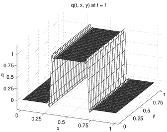
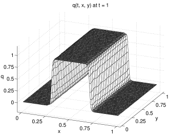
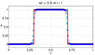
In Figure 1 we show results for a grid of size $60\times 60$ for a fourth-order ($\mathbb{P}_{3}$) method, comparing the choices of $\phi(y)=\min\{1,y\}$ and $\phi(y)=\min\{1,\frac{y}{1.1}\}$. This result shows that the second choice is necessary for pushing our results to multiple dimensions. Other choices exist, but one property we find important is that $\phi(1)<1$. In the remainder of our numerical simulations, we choose $\phi(y)=\min\{1,\frac{y}{1.1}\}$ in all the 2D examples.

(a) $\phi(y)=\min\{1,y\}$

(b) 1D slice of $\phi(y)=\min\{1,y\}$

(c) $\phi(y)=\min\{1,\frac{y}{1.1}\}$

(d) 1D slice of $\phi(y)=\min\{1,\frac{y}{1.1}\}$

Fig. 1: Square wave test case for scalar advection with double periodic boundary conditions. The solution in Panels (a) and (b) is computed using $\phi(y)=\min\{1,y\}$, while the solution in Panels (c) and (d) is computed using $\phi(y)=\min\{1,\frac{y}{1.1}\}$. The simulation is run to a final time of $t=1$, at which point the solution should return to the initial conditions. The choice in (a) and (b) satisfies $\phi(1)=1$, whereas the choice in (c) and (d) satisfies $\phi(1)<1$. The first choice permits oscillations to remain in the solution, whereas the second choice eventually suppresses the unphysical oscillations. The remainder of the simulations used in this work will use the function $\phi(y)=\min\{1,\frac{y}{1.1}\}$.

6 Extensions to systems of equations

As a prototypical example of a hyperbolic system of equations, we consider the compressible Euler equations:

(19) $$\frac{\partial}{\partial t}\begin{bmatrix}\rho\\ \rho{\bf u}\\ \mathcal{E}\end{bmatrix}+\nabla\cdot\begin{bmatrix}\rho{\bf u}\\ \rho{\bf u}{\bf u}+{p}{\mathbb{I}}\\ {\bf u}\left(\mathcal{E}+{p}\right)\end{bmatrix}=0,\qquad\mathcal{E}=\frac{1}{2}\rho\|{\bf u}\|^{2}+\frac{p}{\gamma-1},$$

where $\gamma$ is the gas constant. The conserved and primitive variables are

(20) $$q:=\left(\rho,\rho u^{1},\rho u^{2},\rho u^{3},\mathcal{E}\right)\quad\text{and}\quad w:=\left(\rho,u^{1},u^{2},u^{3},p\right),$$

respectively. In these expressions $\rho$ is the mass density, $\rho{\bf u}:=(\rho u^{1},\rho u^{2},\rho u^{3})$ is the momentum density, $\mathcal{E}$ is the total energy density, ${\bf u}:=(u^{1},u^{2},u^{3})$ is the fluid velocity, and $p$ is the pressure.

The simplest implementation of the proposed limiter for this system would be to apply the scalar limiting procedure to each conserved variable independently. Indeed, our initial tests employed this approach. However, after extensive testing for this system, we discovered that using the primitive variables to define one high-order damping parameter $\theta$ yields better results. An example is provided in Section 6.1 to verify this claim.

The extension of the proposed limiter to systems of equations can be summarized as follows:

Step 0.

Select a set of variables to use in the bounds checking: $w$. In fluid dynamics, primitive variables are the preferred choice due to their Galilean invariance. Select a set of points $\chi_{i}$ that will be used to approximate cell maximum and minimum values. In this work we always select: corners, internal, and edge Gaussian quadrature points.

Step 1.

For each element $i$ and each component $\ell$ of $w$ compute:

(21) $$w^{\ell}_{M_{i}}:=\max_{x\in\chi_{i}}\left\{w^{\ell}(q^{h}(x))\Bigl{|}_{\mathcal{T}_{i}}\right\}\quad\text{and}\quad w^{\ell}_{m_{i}}:=\min_{x\in\chi_{i}}\left\{w^{\ell}(q^{h}(x))\Bigl{|}_{\mathcal{T}_{i}}\right\}.$$

Step 2.

For each element $i$ and each component $\ell$ of $w$ compute an approximate upper and lower bound over the set of neighbors, $N_{\mathcal{T}_{i}}$ (excluding the current cell $\mathcal{T}_{i}$):

(22) $$M^{\ell}_{i} :=\max\left\{\bar{w}^{\ell}_{i}+\alpha(h),\,\max_{j\in N_{\mathcal{T}_{i}}}\left\{w^{\ell}_{M_{j}}\right\}\right\},$$

(23) $$m^{\ell}_{i} :=\min\left\{\bar{w}^{\ell}_{i}-\alpha(h),\,\min_{j\in N_{\mathcal{T}_{i}}}\left\{w^{\ell}_{m_{j}}\right\}\right\},$$

where $\bar{w}^{\ell}_{i}$ is the cell average of ${w}^{\ell}$ over cell $\mathcal{T}_{i}$. $N_{\mathcal{T}_{i}}$. In the Cartesian grid case, we define $N_{\mathcal{T}_{i}}$ to be the set of cells that share a common edge with $\mathcal{T}_{i}$. This provides good results in general, and has the nice property that it does not extend the effective stencil size. For unstructured grids, we define $N_{\mathcal{T}_{i}}$ as the set of all cells that share a common node with $\mathcal{T}_{i}$. If this choice is replaced by elements that share common edges only, then the results are more diffusive.

Step 3.

For each element $i$ compute:

(24) $$\theta_{M_{i}}:=\min_{\ell}\left\{\phi\left(\frac{M^{\ell}_{i}-\bar{w}^{\ell}_{i}}{w^{\ell}_{M_{i}}-\bar{w}^{\ell}_{i}}\right)\right\}\,\,\,\text{and}\,\,\,\theta_{m_{i}}:=\min_{\ell}\left\{\phi\left(\frac{m^{\ell}_{i}-\bar{w}^{\ell}_{i}}{w^{\ell}_{m_{i}}-\bar{w}^{\ell}_{i}}\right)\right\}.$$

Step 4.

For each element $i$ compute:

(25) $$\theta_{i}:=\min\left\{1,\ \theta_{m_{i}},\ \theta_{M_{i}}\right\}.$$

Step 5.

For each element $i$ and each component $\ell$ of $q$ compute

(26) $$\tilde{q}^{h}(x)\Bigl{|}_{\mathcal{T}_{i}}:=\bar{q}_{i}+\theta_{i}\left(q^{h}(x)\Bigl{|}_{\mathcal{T}_{i}}-\bar{q}_{i}\right).$$

Note that we are using the values of the variable $w$ to determine the amount of limiting that needs to be done (i.e., size of $\theta_{i}$), but we are actually applying the limiter to the conserved variables, thereby retaining mass conservation at the discrete level.

6.1 Primitive vs. conservative variables for computing $\theta$: A 1D example

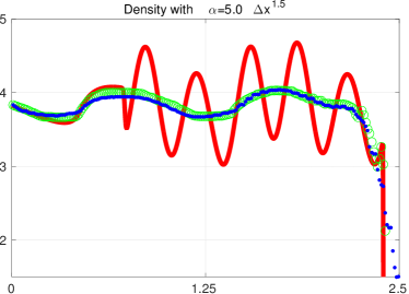
In order to test the limiter performance using either primitive or conservative variables to determine $\theta_{i}$, we consider the one-dimensional shock-entropy problem found in [37, 23, 35], which highlights the interplay between shock-capturing and feature-preservation. The initial conditions for this problem are given by

$$(\rho,u^{1},p)= \begin{cases}\left(3.857143,2.629369,10.3333\right)&x<-4,\\ \left(1+\varepsilon\sin(5x),0,1\right)&x\geq-4.\end{cases}$$

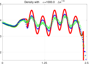
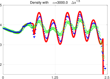
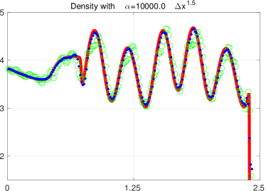
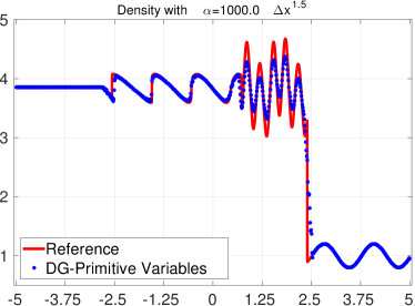
We follow the common practice of setting $\varepsilon=0.2$ and discretize the domain $[-5,5]$ into a total of 200 cells. The final time for this simulation is $t=1.8$. This test problem involves a shockwave interacting with a smooth entropy wave. As this interaction occurs, the result is the formation of highly oscillatory waves after the shock, where high-order accuracy should produce a benefit, yet limiters often smear out these oscillations. Ideally a limiter should be able to pick out and limit only non-physical oscillations, while simultaneously capturing the oscillatory post shock features.

The results of two sets of simulations, one where $\theta_{i}$ is computed from sampling conserved variables and one from sampling primitive variables, is shown in Figure 2. For each version of the limiter, we highlight the effect of the choice of $\alpha$ that permits subcell oscillations to persist. Additionally, we show the full results of this problem with the primitive variables used to compute $\theta_{i}$ and $\alpha=500h^{1.5}$ in Figure 3. These results clearly show the advantage of using primitive variables in defining $\theta_{i}$ and give a range of $\alpha$ values that seem to give good results.

In every simulation past this point we use primitive variables to define the rescaling parameter and we take $\alpha=500h^{1.5}$, which seems to balance the need to suppress unphysical oscillations and still retain high-order accuracy in smooth regions. The only exception to this is the example in Section 8.3, where for most of the computational domain we do use the primitive variables to calculate $\theta_{i}$, but there is a small region around the corner of the backward-facing step where we switch to a more aggressive limiter based on conservative variables.

Fig. 2: Shock-entropy problem with $4$ points plotted per cell. In these panels we highlight the benefit of using the primitive variables to conduct the limiting at negligible additional cost. To highlight the study, we compare different results that are constructing by modifying the subcell tolerance parameter $\alpha$. We observe that selecting a relatively large value of $\alpha$ combined with primitive variables is our best choice, given that the conserved variables tend to introduce additional oscillations post shock in smooth regimes.

Fig. 3: The full plot of the shock-entropy wave problem with $\alpha=500h^{1.5}$ and primitive variable limiting. This $\alpha$ value seems to give a good compromise of resolution and limiting. We will use $\alpha=500h^{1.5}$ in our future calculations unless otherwise noted.

6.2 On the importance of $\alpha$: A simple 2D case study

The convergence properties shown in Section 4.3 should still be observable in 2D and for systems. To verify this we consider a 2D Euler example that has a smooth exact solution. This example involves an ideal gas with $\gamma=1.4$, on $(x,y)\in[0,2]\times[0,2]$ with double-periodic boundary conditions and the following initial conditions:

(27) $$\left(\rho,u^{1},u^{2},p\right)=\bigl{(}1+0.2\sin(\pi(x+y)),0.7,0.3,1.0\bigr{)}.$$

In the exact solution $u^{1}$, $u^{2}$, and $p$ remain constant for all space and time, while the density, $\rho$, is advected with the constant fluid velocity given by $(u_{1},u_{2})=(0.7,0.3)$. The numerical $L_{2}$ errors after one revolution (i.e., time $t=2$) are shown in Table 2. To produce these results we used the same time-stepping scheme as in Section 4.3. We again observe that we must have a nonzero value of $\alpha$ to asymptotically match the unlimited solution’s convergence even for this very simple test problem.

Mesh	No Limiter	Order	$\alpha=0$	Order	$\alpha=0.5h^{1.5}$	Order
$10$	$1.81\times 10^{-05}$	—	$4.24\times 10^{-02}$	—	$1.07\times 10^{-02}$	—
$15$	$3.39\times 10^{-06}$	$4.97$	$3.12\times 10^{-02}$	$0.92$	$6.07\times 10^{-03}$	$1.68$
$22$	$6.87\times 10^{-07}$	$4.48$	$2.23\times 10^{-02}$	$0.94$	$2.12\times 10^{-03}$	$2.95$
$33$	$1.33\times 10^{-07}$	$4.05$	$1.75\times 10^{-02}$	$0.59$	$8.56\times 10^{-05}$	$7.91$
$50$	$2.50\times 10^{-08}$	$4.36$	$1.12\times 10^{-02}$	$1.17$	$2.50\times 10^{-08}$	$21.25$
$75$	$4.91\times 10^{-09}$	$4.02$	$7.84\times 10^{-03}$	$0.88$	$4.91\times 10^{-09}$	$4.02$
$113$	$9.52\times 10^{-10}$	$4.15$	$5.11\times 10^{-03}$	$1.08$	$9.52\times 10^{-10}$	$4.15$

Table 2: Convergence for the 2D Euler equation problem from Section 6.2. All errors are $L_{2}$ norm errors. We see that with a nonzero value of $\alpha$, we eventually match the unlimited problem’s convergence rate, but that without a nonzero value of $\alpha$, the convergence is very poor. In fact when the other methods are showing their theoretical asymptotic convergence rates the method using $\alpha=0$ is still showing first order convergence (it should be able to achieve second order convergence).

7 Positivity preservation

Given the framework of the limiter, the inclusion of the recent and popular positivity-preserving methods developed by Zhang and Shu [46] is essentially automatic. For example, to guarantee positivity of a scalar function that has a positive mean, we simply replace the computation of the rescaling parameter in equation (12) of Step 4 of the algorithm with an additional term to take the minimum over:

$$\theta_{i}=\min\left\{1,\ \theta_{m_{i}},\ \theta_{M_{i}},\,\frac{\bar{q}_{i}}{\bar{q}_{i}-q_{m_{i}}}\right\}.$$

Extensions to the compressible Euler equations to maintain positive pressure require expanding the unknown variables as a quadratic function of $\theta$. The details of this can be found in the work of Zhang and Shu [46].

8 Additional numerical results

In this section we apply our numerical scheme to several additional standard numerical test cases. We include one and two-dimensional test cases on both Cartesian and unstructured grids. These benchmark test cases are used to verify the accuracy and robustness of the proposed method.

8.1 2D Riemann problems

First, we consider two multidimensional Riemann problem test cases. These problems have been used extensively as benchmark test cases for other limiters [17, 6].

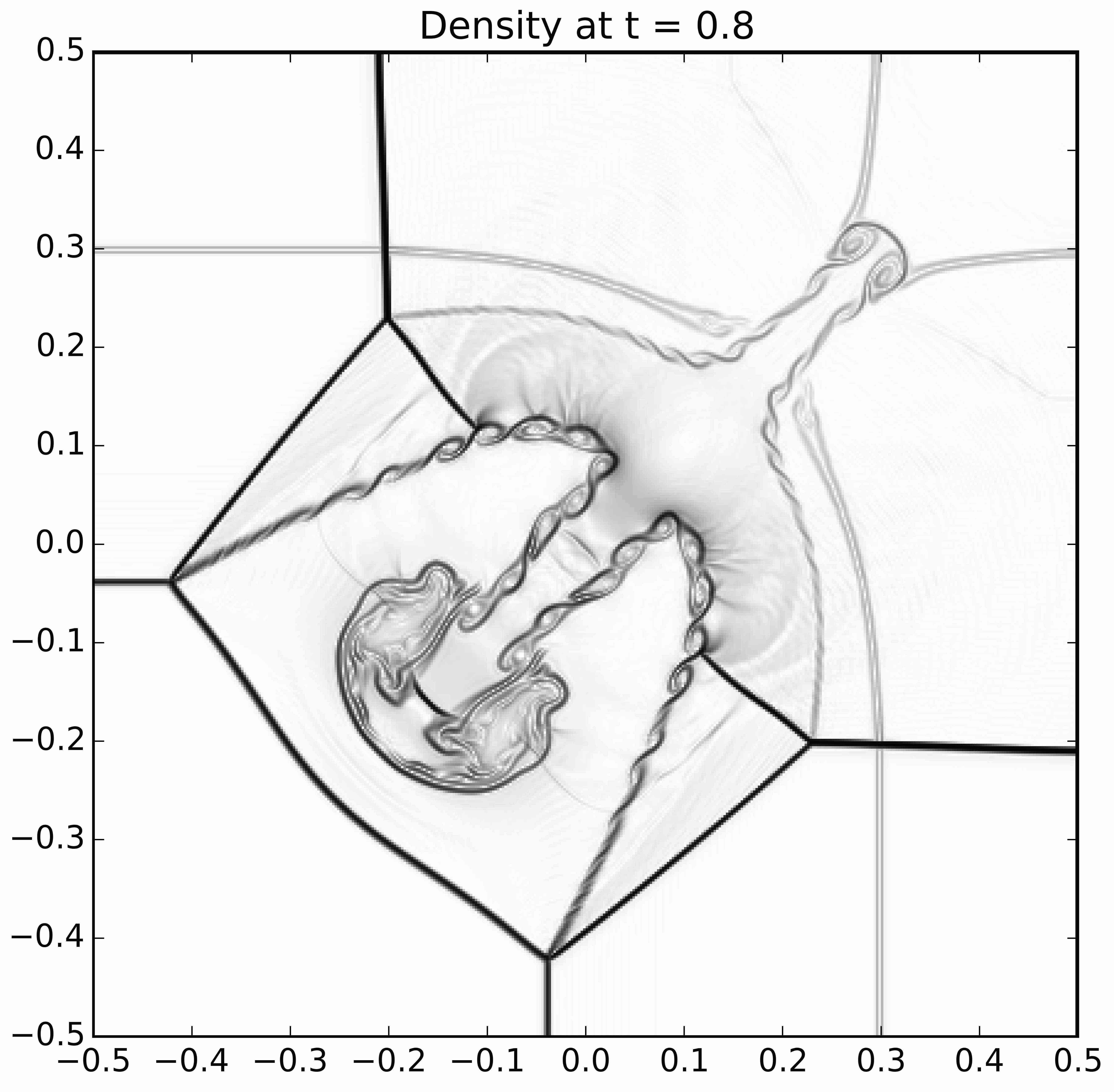
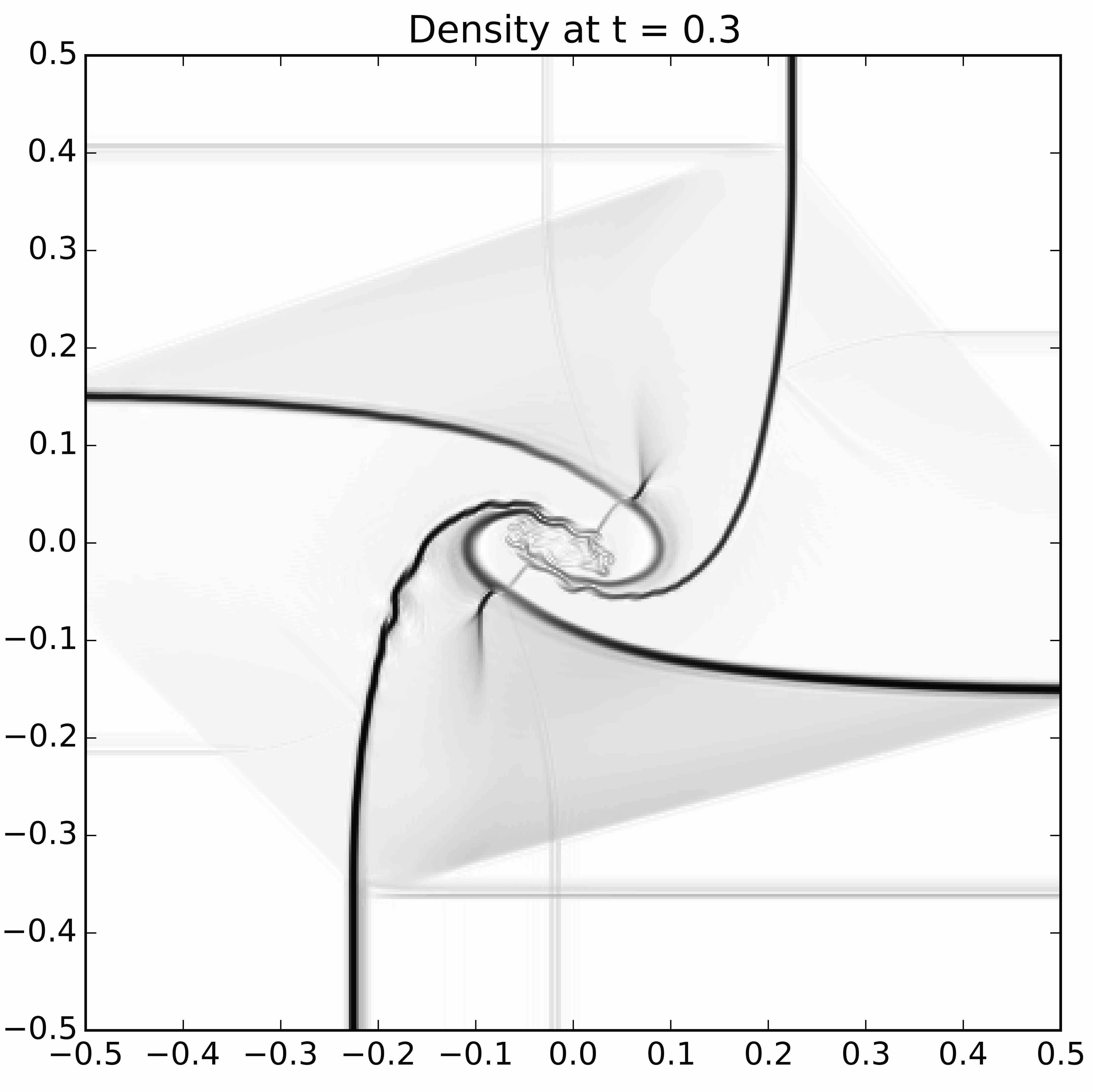
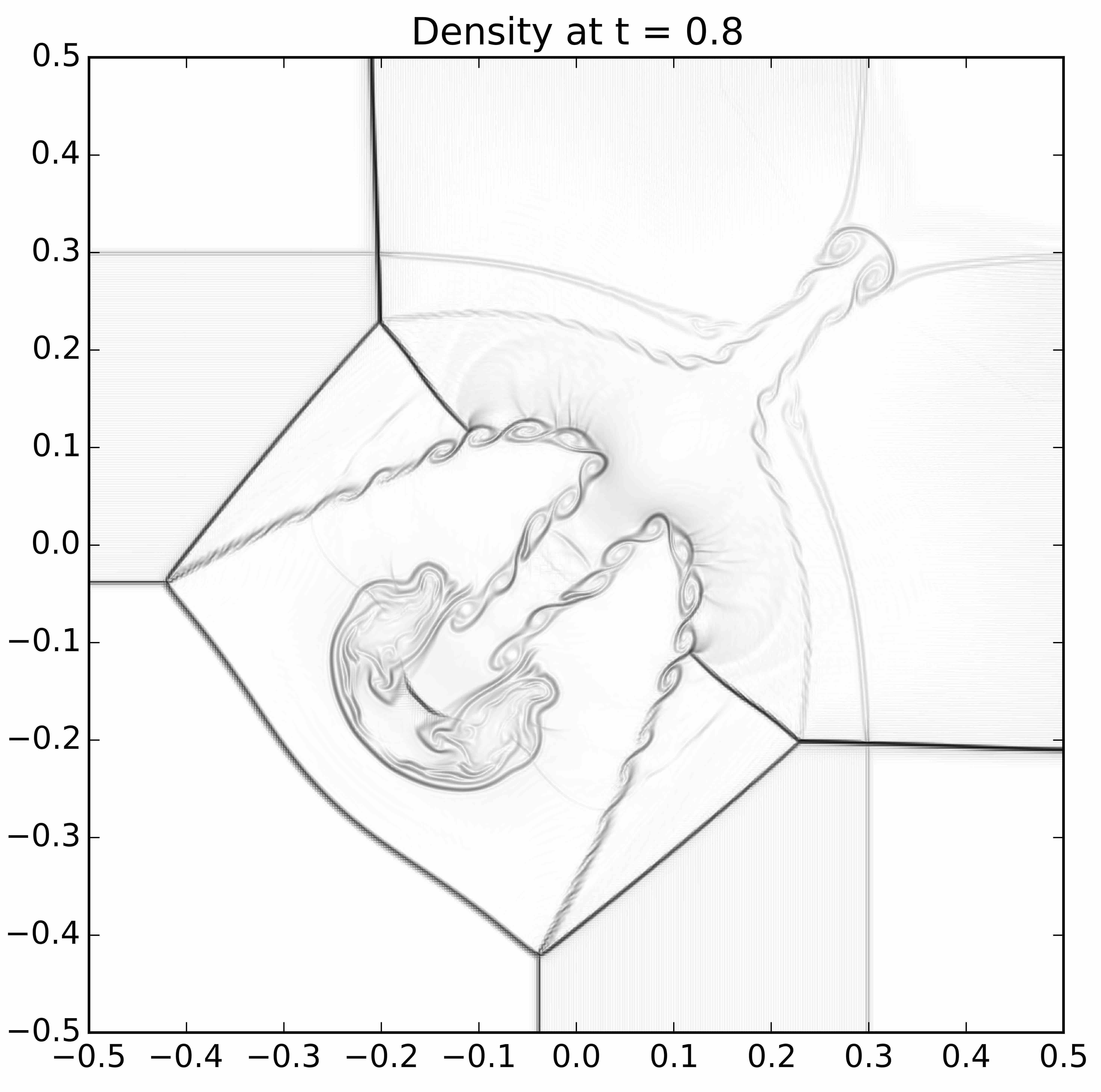
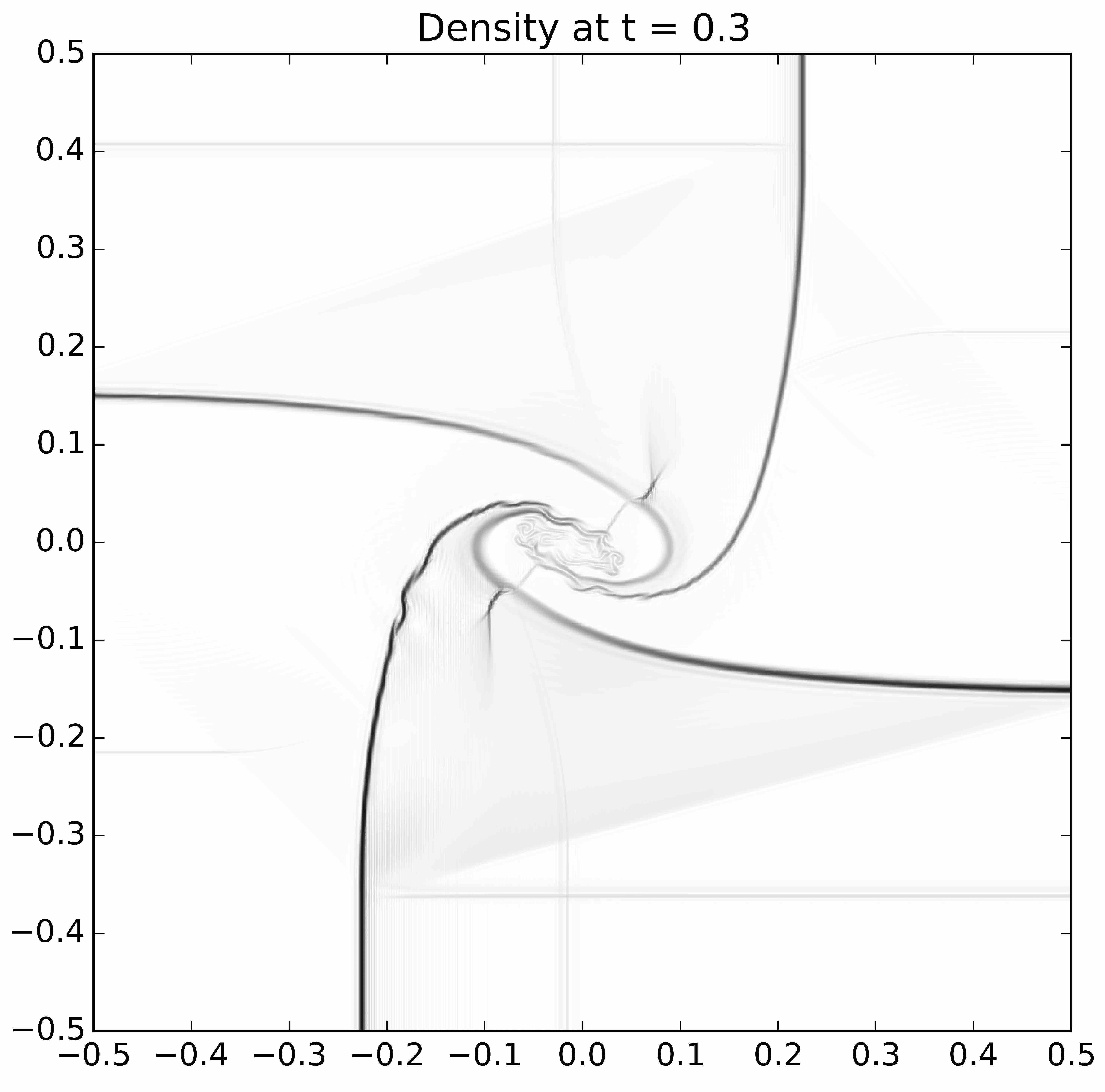
The first example, ${\bf RP1}$, is a well known example that can be found in [34] and [21]. We divide the domain $[-0.5,0.5]\times[-0.5,0.5]$ into four rectangular quadrants, all of which meet at the point $(0.3,0.3)$. We number the quadrants starting in the upper left hand corner, and continue in a counterclockwise manner. For example, the upper left hand corner is Quadrant 1, and the upper right hand corner is Quadrant $4$. The initial conditions for RP1 are defined in Table 3.

Quadrant	$\rho$	$u^{1}$	$u^{2}$	$p$	$\rho$	$u^{1}$	$u^{2}$	$p$
1	$0.5323$	$1.2060$	$0.0000$	$0.3000$	$2.00$	$0.75$	$0.50$	$1.00$
2	$0.1380$	$1.2060$	$1.2060$	$0.0290$	$1.00$	$-0.75$	$0.50$	$1.00$
3	$0.5323$	$0.0000$	$1.2060$	$0.3000$	$3.00$	$-0.75$	$-0.50$	$1.00$
4	$1.5000$	$0.0000$	$0.0000$	$1.5000$	$1.00$	$0.75$	$-0.50$	$0.00$

Table 3: Initial conditions for RP1 (columns 2–5) and RP3 (columns 6–9).

The second two-dimensional Riemann problem we consider is called RP3 [17, 6]. The domain $[-0.5,0.5]\times[-0.5,0.5]$ is divided into four equal area quadrants, and the numbering of the quadrants is also defined in a counterclockwise fashion starting at the upper left hand corner. The initial conditions for RP3 are defined in Table 3.

We run both of these examples on a grid with $400\times 400$ elements and use third-order ${\mathbb{P}}_{2}$ elements. Time-stepping was done with the classical third-order SSPRK3 method using a CFL number of $0.1$. Both examples are run using a Rusanov (local Lax Friedrichs (LLF)) flux [33]. Results are plotted in Figure 4, which are schlieren plots that show the magnitude of the gradient of the solution density $|\nabla\rho|$. We show two figures, one with 1 point per cell and the other with three points per direction per cell. We make this comparison because the limiter permits tiny oscillations to remain in the solution, since it ignores all variations smaller than a certain threshold (controlled by the parameter $\alpha$). As the mesh is refined, $\alpha$ also shrinks, and therefore the oscillations will vanish with mesh refinement. We note that these oscillations are not visible in the plots showing one point per cell.

(a) Density for RP1 at $t=0.8$. One point per cell.

(b) Density for RP3 at $t=0.3$. One point per cell.

(c) Density for RP1 at $t=0.8$. Nine points per cell.

(d) Density for RP3 at $t=0.3$. Nine points per cell.

Fig. 4: 2D Riemann problems. For RP1 $30$ contours equally spaced between $0.3$ and $1.8$ are plotted. For RP3 $30$ contours equally spaced between $0.1$ and $3.3$ are plotted.

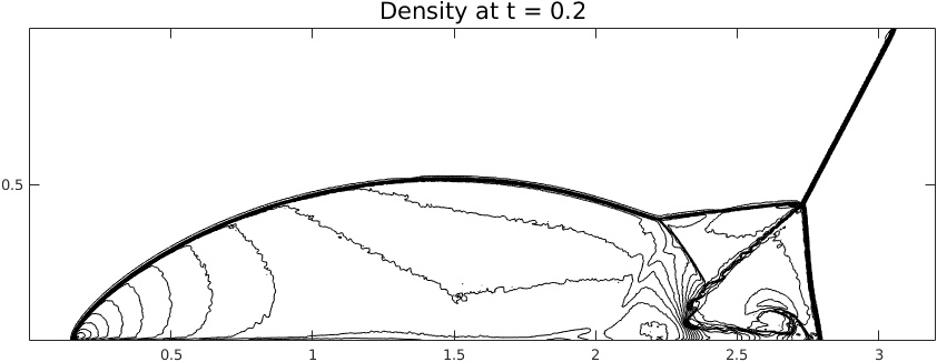
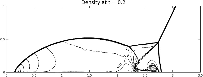
8.2 Double Mach reflection

For our next two-dimensional example, we run the classical double Mach reflection test problem (e.g., see Qiu and Shu [30]). In this test problem a Mach $10$ shock approaches a wedge with an angle of $30$ degrees. In order to simplify the implementation of this problem on a Cartesian grid, it is typical to rotate the whole problem so that the wedge conforms to the bottom boundary. The problem is run on the domain $[0,3.2]\times[0,1]$. For the bottom boundary we impose the exact solution for $x<\frac{1}{6}$ and we enforce solid wall boundary conditions for $x\geq\frac{1}{6}$. The initial conditions are

$$\left(\rho,u^{1},u^{2},p\right)=\begin{cases}\left(8.0,8.25,\cos\left(\frac{\pi}{6}\right),8.25\sin\left(\frac{\pi}{6}\right),116.5\right)&\text{if}\quad x<\frac{1}{6},\\ \left(1.4,0,0,1\right)&\text{otherwise.}\end{cases}$$

In the Cartesian case we run this test using a $960\times 240$ cell grid matching the second highest resolution in[30]. In the unstructured grid case we use an example with $204,479$ cells. Both examples are run with the 10-stage SSPRK4 method with a CFL constant of $0.08$. This smaller CFL number was chosen to guarantee positivity of the solution.

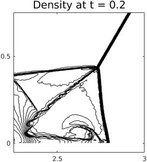
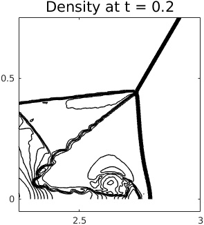
This problem is challenging given that there is a complicated strong-shock structure, as well as a region where there is vortical flow. It can be seen in Figure 5 that both limiters essentially succeed in capturing this behavior. The unstructured grid example appears much better than the Cartesian grid example; this is be due to the fact that the unstructured grid example makes use of all cells touching a current cell, and on the Cartesian grid we only use cells sharing an edge. This was done because ideally we do not want to introduce any extra communication in our limiter (by communicating across corners). However in the unstructured grid case just limiting using cells sharing edges is not good enough and so the unstructured grid limiter had to make use of values in cells sharing nodes instead of edges. In Figure 6 we see a close of up the solution in the vortical flow region. Both solutions are certainly forming vortices but the unstructured grid again seems to give much better behavior. However neither example quite matches the maximum rollup seen in the comparable resolution examples in [30].

(a) Cartesian grid

(b) Unstructured grid

Fig. 5: Double Mach reflection. For this example we used an $\alpha$ equal to $1000h^{1.5}$. We plot a total of $30$ contours that range equispaced from $1.5$ to $22.7$. Both plots were done using one point per cell.

(a) $\mathbb{P}_{3}$ on a Cartesian grid

(b) $\mathbb{P}_{3}$ unstructured grid

Fig. 6: The output from Figure 5 zoomed in to show the resolution near the contact discontinuity. This contact discontinuity displays the roll up behavior that is expected in high resolution numerical simulations

8.3 Mach 3 wind tunnel with a step on Cartesian and unstructured meshes

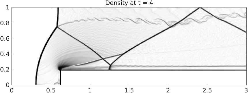
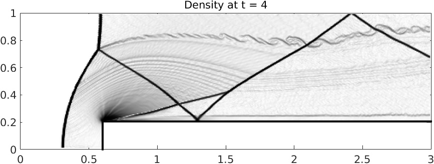
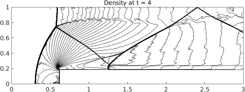
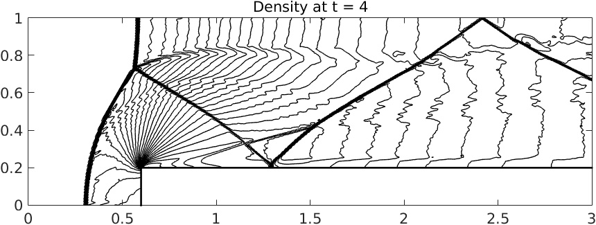
We next consider a classical test problem [43, 14] that is often overlooked, likely due to its difficulty. The problem involves an ideal gas with $\gamma=1.4$ and a strong shock moving at Mach $3$ that passes past a forward facing step. The initial conditions for this problem are given by $\left(\rho,u^{1},u^{2},p\right)=\left(1.0,3.0,0.0,{\gamma}^{-1}\right).$ The computational domain is the rectangle $[0,3]\times[0,1]$ with the region $[0.6,3.0]\times[0.0,0.2]$ cut out. In the Cartesian grid case, we use a uniform grid with $480\times 160$ elements, and we use a total of $90,342$ cells for the unstructured grid case. The Cartesian grid matches the moderately refined implementation in [3], however we run with the higher-order $\mathbb{P}_{3}$ elements instead of $\mathbb{P}_{2}$ elements used in [3]. Both examples are run with SSPRK4 using the LLF flux and a CFL of $0.4$.

This is a complicated problem featuring a long contact discontinuity where, again, vortices that should form are observable with high-resolution simulations. An additional and well-known difficulty is that this example tends to form a spurious entropy layer above the step. This results in the creation of a stem-like structure where there would normally be a shock reflecting off of the step. This is especially noticeable in the Cartesian grid plot. To mitigate this effect, we use a slightly more aggressive implementation of our limiter near top of the step. In place of using point-wise values of the primitive variables to estimate local upper and lower bounds, we use cell averages of the conserved variables in this edge region only. That is, we replace $M^{\ell}_{i}$ and $m^{\ell}_{i}$ in equations (22) and (23) by

$$M_{i}:=\max\left\{\bar{q}_{i}+\alpha(h),\,\max_{j\in N_{\mathcal{T}_{i}}}\left\{\bar{q}^{h}_{M_{j}}\right\}\right\}\,\text{ and }\,m_{i}:=\min\left\{\bar{q}_{i}-\alpha(h),\,\min_{j\in N_{\mathcal{T}_{i}}}\left\{\bar{q}^{h}_{m_{j}}\right\}\right\},$$

where the $\ell$ superscript has been suppressed. Note that this means that in this special region we are not using the primitive variables for determining $\theta_{i}$, but actually the conserved variables; furthermore, we are using the average values $\bar{q}$ rather than point values at the points defined by $\chi_{i}$. Additionally we use a much smaller $\alpha$ value in this region to obtain better results. In the majority of the domain we take $\alpha=500h^{1.5}$, but in the small region above the step we take $\alpha=20h^{1.5}$. The region using the more aggressive limiter extends $6$ cells above the step in the Cartesian grid case, and until $y=0.24$ above the step in the unstructured grid case. These values can certainly be modified, but we found that if the region is taken to be only one cell width, then the entropy layer tends to be much more prominent. Moreover, if the more aggressively limited region is too large the shocks in the problem will be smeared out too heavily.

In Figures 7 and 8 we observe that both methods do an excellent job of capturing the structure of the contact discontinuity. However it appears that the Cartesian grid case suffers from a pronounced spurious entropy layer; although it should be noted that the entropy layer is not atypically large (e.g., see [3, 51]). Given the relative simplicity of this limiter the results seem very promising.

(a) Cartesian grid

(b) Unstructured grid

Fig. 7: Density schlieren plots from the forward facing step problem run on Cartesian and unstructured grids. The Cartesian grid used $h=\frac{1}{160}$, and the unstructured grid used $90,342$ cells (that were uniformly sized). Both were plotted with one point per cell.

(a) Cartesian grid

(b) Unstructured grid

Fig. 8: Density contour plots from the forward facing step problem run on Cartesian and unstructured grids. There are $30$ contours spaced evenly from $0.1$ to $4.54$.

9 Conclusions

In this work, we have presented a novel limiter for the discontinuous Galerkin method. It is the first of its kind given its ease of implementation, ability to retain high-order accuracy, and robustness for simulation problems with strong shocks. The results are achieved without the need for an additional shock-detector. The proposed method can be viewed as either an extension of the Barth-Jespersen [2] limiter to discontinuous Galerkin methods or as extending the Zhang and Shu [46] positivity preserving method to be able to accommodate shocks and not just satisfy the positivity principle. Several numerical results were presented, including single and multidimensional examples on Cartesian and unstructured grids. Future work will involve investigating the ability of this limiter to work on more complicated hyperbolic problems such as magnetohydrodynamics (MHD) and three dimensional problems with structured and unstructured grids.

Acknowledgements. The work of SAM was supported in part by NSF grant DMS–1216732. The work of JAR was supported in part by NSF grant DMS–1419020.

References

- [1] H. Abbassi, F. Mashayek, and G.B. Jacobs. Shock capturing with entropy-based artificial viscosity for staggered grid discontinuous spectral element method. Comput. & Fluids, 98:152–163, 2014.
- [2] T.J. Barth and D.C. Jespersen. The design and application of upwind schemes on unstructured meshes. AIAA-89-0366, 1989.
- [3] B. Cockburn and C.-W. Shu. The Runge-Kutta discontinuous Galerkin method for conservation laws. V. Multidimensional systems. J. Comput. Phys., 141(2):199–224, 1998.
- [4] B. Cockburn and C.-W. Shu. Runge-Kutta discontinuous Galerkin methods for convection-dominated problems. J. Sci. Comput., 16(3):173–261, 2001.
- [5] P. Colella and M.D. Sekora. A limiter for PPM that preserves accuracy at smooth extrema. J. Comput. Phys., 227(15):7069–7076, 2008.
- [6] M. Dumbser, O. Zanotti, R. Loubère, and S. Diot. A posteriori subcell limiting of the discontinuous Galerkin finite element method for hyperbolic conservation laws. J. Comput. Phys., 278:47–75, 2014.
- [7] S.K. Godunov. A difference method for numerical calculation of discontinuous solutions of the equations of hydrodynamics. Mat. Sb., 47:271–306, 1959.
- [8] S. Gottlieb, C.-W. Shu, and E. Tadmor. Strong stability-preserving high-order time discretization methods. SIAM Rev., 43(1):89–112, 2001.
- [9] A. Harten. High resolution schemes for hyperbolic conservation laws. J. Comput. Phys., 49:357–393, 1983.
- [10] A. Harten. On a class of high resolution total-variation-stable finite-difference schemes. SIAM Journal on Numerical Analysis, 21(1):1–23, 1984.
- [11] J.S. Hesthaven and T. Warburton. Nodal Discontinuous Galerkin Methods: Algorithms, Analysis, and Applications. Springer, 2007.
- [12] H. Hoteit, Ph. Ackerer, R. Mosé, J. Erhel, and B. Philippe. New two-dimensional slope limiters for discontinuous Galerkin methods on arbitrary meshes. Internat. J. Numer. Methods Engrg., 61(14):2566–2593, 2004.
- [13] H. Hoteit, Ph. Ackerer, R. Mosé, J. Erhel, and B. Philippe. New two-dimensional slope limiters for discontinuous Galerkin methods on arbitrary meshes. Internat. J. Numer. Methods Engrg., 61(14):2566–2593, 2004.
- [14] G.-S. Jiang and C.-W. Shu. Efficient implementation of weighted ENO schemes. J. Comput. Phys., 126(1):202–228, 1996.
- [15] D.I. Ketcheson. Highly efficient strong stability-preserving Runge-Kutta methods with low-storage implementations. SIAM J. Sci. Comput., 30(4):2113–2136, 2008.
- [16] L. Krivodonova. Limiters for high-order discontinuous Galerkin methods. J. Comput. Phys., 226(1):879–896, 2007.
- [17] A. Kurganov and E. Tadmor. Solution of two-dimensional riemann problems for gas dynamics without Riemann problem solvers. Numerical Methods for Partial Differential Equations, 18(5):584–608, 2002.
- [18] D. Kuzmin. A vertex-based hierarchical slope limiter for -adaptive discontinuous Galerkin methods. J. Comput. Appl. Math., 233(12):3077–3085, 2010.
- [19] D. Kuzmin. Slope limiting for discontinuous Galerkin approximations with a possibly non-orthogonal Taylor basis. Internat. J. Numer. Methods Fluids, 71(9):1178–1190, 2013.
- [20] D. Kuzmin. Hierarchical slope limiting in explicit and implicit discontinuous Galerkin methods. J. Comput. Phys., 257(part B):1140–1162, 2014.
- [21] R.J. LeVeque. Wave propagation algorithms for multidimensional hyperbolic systems. J. Comput. Phys., 131(2):327–353, 1997.
- [22] R.J. LeVeque. Finite Volume Methods for Hyperbolic Problems. Cambridge University Press, 2002.
- [23] X.-D. Liu, S. Osher, and T. Chan. Weighted essentially non-oscillatory schemes. J. Comput. Phys., 115(1):200–212, 1994.
- [24] H. Luo, J.D. Baum, and R. Löhner. A Hermite WENO-based limiter for discontinuous Galerkin method on unstructured grids. J. Comput. Phys., 225(1):686–713, 2007.
- [25] K. Michalak and C. Ollivier-Gooch. Limiters for unstructured higher-order accurate solutions of the Euler equations. AIAA 2008-776, 2008.
- [26] P.-O. Persson and J. Peraire. Sub-cell shock capturing for discontinuous galerkin methods. AIAA 2006-112, 2006.
- [27] J. Qiu and C.-W. Shu. Hermite WENO schemes and their application as limiters for Runge-Kutta discontinuous Galerkin method: One-dimensional case. J. Comput. Phys., 193(1):115–135, 2004.
- [28] J. Qiu and C.-W. Shu. A comparison of troubled-cell indicators for Runge-Kutta discontinuous Galerkin methods using weighted essentiall nonoscillatory limiters. SIAM J. Sci. Comput., 27:995–1013, 2005.
- [29] J. Qiu and C.-W. Shu. Hermite WENO schemes and their application as limiters for Runge-Kutta discontinuous Galerkin method. II. Two dimensional case. Comput. & Fluids, 34(6):642–663, 2005.
- [30] J. Qiu and C.-W. Shu. Runge-Kutta discontinuous Galerkin method using WENO limiters. SIAM J. Sci. Comput., 26(3):907–929, 2005.
- [31] W.H. Reed and T.R. Hill. Triangular mesh methods for the neutron transport equation. Technical Report LA-UR-73-479, Los Alamos Scientific Laboratory, 1973.
- [32] J.A. Rossmanith. DoGPack software, 2015. Available from http://www.dogpack-code.org.
- [33] V.V. Rusanov. Calculation of interaction of non-steady shock waves with obstacles. J. Comp. Math. Phys. USSR, 1:267–279, 1961.
- [34] C.W. Schulz-Rinne, J.P. Collins, and H.M. Glaz. Numerical solution of the Riemann problem for two-dimensional gas dynamics. SIAM J. Sci. Comput., 14(6):1394–1414, 1993.
- [35] D. C. Seal, Y. Güçlü, and A. J. Christlieb. The Picard integral formulation of weighted essentially non-oscillatory schemes. SIAM J. Numer. Anal., 2014. (accepted).
- [36] D.C. Seal. Discontinuous Galerkin methods for Vlasov models of plasma. PhD thesis, University of Wisconsin-Madison, Madison, WI, 2012.
- [37] C.-W. Shu and S. Osher. Efficient implementation of essentially nonoscillatory shock-capturing schemes. II. J. Comput. Phys., 83(1):32–78, 1989.
- [38] P.K. Sweby. High resolution schemes using flux limiters for hyperbolic conservation laws. SIAM J. Numer. Anal., 21(5):995–1011, 1984.
- [39] E. Tadmor. Convenient total variation diminishing conditions for nonlinear difference schemes. SIAM J. Numer. Anal., 25(5):1002–1014, 1988.
- [40] B. van Leer. Towards the ultimate conservative difference scheme I. The quest of monotonicity. In H. Cabannes and R. Temam, editors, Proceedings of the Third International Conference on Numerical Methods in Fluid Mechanics, volume 18, pages 163–168, 1973.
- [41] B. van Leer. Towards the ultimate conservative difference scheme. ii. monotonicity and conservation combined in a second-order scheme. J. Comput. Phys., 14(4):361–370, 1974.
- [42] J. von Neumann and R. Richtmyer. A method for the numerical calculation of hydrodynamic shocks. J. Applied Physics, 21:232–237, 1950.
- [43] P. Woodward and P. Colella. The numerical simulation of two-dimensional fluid flow with strong shocks. J. Comput. Phys., 54(1):115–173, 1984.
- [44] M. Yang and Z.J. Wang. A parameter-free generalized moment limiter for high-order methods on unstructured grids. Adv. Appl. Math. Mech., 1(4):451–480, 2009.
- [45] J. Yu and C. Yan. An artificial diffusivity discontinuous Galerkin scheme for discontinuous flows. Comput. & Fluids, 75:56–71, 2013.
- [46] X. Zhang and C.-W. Shu. Maximum-principle-satisfying and positivity-preserving high-order schemes for conservation laws: survey and new developments. Proc. R. Soc. A, 467(2134):2752–2776, 2011.
- [47] X. Zhang and C.-W. Shu. A minimum entropy principle of high order schemes for gas dynamics equations. Numerische Mathematik, 121:545–563, 2012.
- [48] J. Zhu and J. Qiu. Hermite WENO schemes and their application as limiters for Runge-Kutta discontinuous Galerkin method. III. Unstructured meshes. J. Sci. Comput., 39(2):293–321, 2009.
- [49] J. Zhu and J. Qiu. WENO schemes and their application as limiters for RKDG methods based on trigonometric approximation spaces. J. Sci. Comput., 55(3):606–644, 2013.
- [50] J. Zhu, J. Qiu, C.-W. Shu, and M. Dumbser. Runge-Kutta discontinuous Galerkin method using WENO limiters. II. Unstructured meshes. J. Comput. Phys., 227(9):4330–4353, 2008.
- [51] J. Zhu, X. Zhong, C.-W. Shu, and J. Qiu. Runge-Kutta discontinuous Galerkin method using a new type of WENO limiters on unstructured meshes. J. Comput. Phys., 248:200–220, 2013.